The Carnegie-Spitzer-IMACS Redshift Survey of Galaxy Evolution since $z=1.5$: I. Description and Methodology

Abstract

We describe the Carnegie-Spitzer-IMACS (CSI) Survey, a wide-field, near-IR selected spectrophotometric redshift survey with the Inamori Magellan Areal Camera and Spectrograph (IMACS) on Magellan-Baade. By defining a flux-limited sample of galaxies in Spitzer IRAC $3.6\mu$m imaging of SWIRE fields, the CSI Survey efficiently traces the stellar mass of average galaxies to $z\sim 1.5$. This first paper provides an overview of the survey selection, observations, processing of the photometry and spectrophotometry. We also describe the processing of the data: new methods of fitting synthetic templates of spectral energy distributions are used to derive redshifts, stellar masses, emission line luminosities, and coarse information on recent star-formation. Our unique methodology for analyzing low-dispersion spectra taken with multilayer prisms in IMACS, combined with panchromatic photometry from the ultraviolet to the IR, has yielded high quality redshifts for 43,347 galaxies in our first 5.3 degs² of the SWIRE XMM-LSS field. We use three different approaches to estimate our redshift errors and find robust agreement. Over the full range of $3.6\mu$m fluxes of our selection, we find typical redshift uncertainties of $\sigma_{z}/(1+z)\lesssim 0.015$. In comparisons with previously published spectroscopic redshifts we find scatters of $\sigma_{z}/(1+z)=0.011$ for galaxies at $0.7\leq z\leq 0.9$, and $\sigma_{z}/(1+z)=0.014$ for galaxies at $0.9\leq z\leq 1.2$. For galaxies brighter and fainter than $i=23$ mag, we find $\sigma_{z}/(1+z)=0.008$ and $\sigma_{z}/(1+z)=0.022$, respectively. Notably, our low-dispersion spectroscopy and analysis yields comparable redshift uncertainties and success rates for both red and blue galaxies, largely eliminating color-based systematics that can seriously bias observed dependencies of galaxy evolution on environment.

1. Introduction

Understanding the evolution of galaxies and large scale structure remains a fundamental challenge in astrophysics. Many ambitious galaxy surveys have been carried out to address this problem, but limited time on large telescopes results in a classic problem: sky coverage, depth, and spectral resolution – choose two. For example, the very-wide-area Sloan Digital Sky Survey (SDSS) provides a wealth of spectral information for galaxies over a cosmologically significant volume, but its modest depth limits the SDSS to the relatively local, ‘modern’ universe. Conversely, the Hubble Ultra-Deep Field photometric survey probes deep into cosmic time — to the epoch of reionization, but only over a tiny volume whose small population of galaxies leads to large uncertainties on their physical properties. While the union of such surveys has begun to paint a coherent picture of galaxy growth, significant patches of blank canvas limit our ability to fully describe how environmental processes, the infall of gas that fuels star formation, galaxy mergers and acquisitions, and feedback, all shape the evolution of galaxies over cosmic time.

The Carnegie-Spitzer-IMACS Survey (CSI) has been designed to address one of the most dramatic and least understood features of galaxy evolution — the remarkably rapid decline in cosmic star formation since $z\sim 1.5$. It is during this extended epoch of galaxy maturation that galaxy groups and clusters have also emerged as a conspicuous feature of the landscape. The CSI Survey is uniquely able to link together the evolution of individual galaxies with these features of large-scale structure growth.

In our ambitious spectrophotometric redshift survey of distant galaxies, we strike a balance between the aforementioned three factors: (1) high completeness to moderate redshift ($z\lower 1.29167pt\hbox{$\scriptscriptstyle\;\buildrel<\over{\sim}\;$}1.5$), (2) spectral resolution intermediate between conventional photometric and spectroscopic surveys (combining the efficiency of imaging surveys with a spectral resolution high enough to resolve large-scale structure and prominent emission-lines); and (3) an unprecedented area of 15 deg² for a $z\lower 1.29167pt\hbox{$\scriptscriptstyle\;\buildrel>\over{\sim}\;$}1$ survey. These give the CSI Survey a volume comparable to the SDSS, with a selection method that efficiently traces stellar mass over 2/3 the age of the universe ($0.4<z<1.5$) — spanning the critical redshift range where cosmic star formation precipitously drops, and groups and clusters become prominent. As the redshift survey with the largest unbiased volume at $z=1$, CSI will allow us to comprehensively address the interplay between environment, galaxy mass buildup, and star formation at these redshifts.

The innovation of moving to low resolution for cosmologically interesting problems of galaxy evolution was instigated by the PRIMUS collaboration (e.g. Coil et al., 2011; Cool et al., 2013). They designed a low dispersion prism to perform an optically selected redshift survey of several legacy fields and have used their sample of 140,000 galaxies to constrain the evolution of galaxy stellar mass functions (Moustakas et al., 2013), and to study AGN activity (Mendez et al., 2013) and it’s relation to galaxy evolution (Aird et al., 2012, 2013).

In this, the sample definition and basic analysis paper of the CSI Survey, we describe the design of the project, with particular focus on the flux limits of the selection, the data processing and the spectral energy distribution (SED) fitting with its attendant determination of redshifts and redshift errors. We apply our methodologies to the first batch of data in 5.3 degs² of the SWIRE XMM-LSS field, and provide an overview of some basic properties of galaxies over the past 9 Gyr, with an emphasis on the gains made by selecting galaxies by stellar mass instead of by their rest-frame UV light.

2. The Carnegie-Spitzer-IMACS Survey

2.1. The limitations of optically-selected surveys

Any effective probe of galaxy assembly must sample a wide range of masses in order to trace evolutionary connections between large and small systems. The build-up of massive red sequence galaxies may be driven by mergers with sub-$M^{*}$ systems, so it is essential to trace evolution to masses below $M^{*}$ to mitigate against the differential growth of the high- and low-mass populations. This trade-off between depth and area noted above has led to a dichotomy in redshift surveys. Narrow and deep programs, such as the Gemini Deep Deep Survey (GDDS; Abraham et al., 2004) or the Galaxy Mass Assembly Ultra-deep Spectroscopic Survey (GMASS; Halliday et al., 2008) could not cover enough volume to robustly sample the evolution of the high mass population at $z<1$, while other surveys that have traded depth for area do not reach below $M^{*}$ with high fidelity.

An old stellar population at $z=1$ with a stellar mass of $10^{11}M_{\odot}$ corresponds to roughly $i=23$ mag and $r=24$ mag in the optical, as shown in Figure 1. The extreme optical faintness of such galaxies results in many of them being missed in optically-selected surveys despite their relatively high masses. For example, the selection limits for DEEP2 (Willmer et al., 2006) and PRIMUS (Coil et al., 2011) are shown in this figure by the blue and green dashed lines, respectively. At $z>1$ these programs required galaxies to be extremely massive or have their optical light dominated by young stellar populations in order to be fall within the survey selection. At best it can be difficult to trace the evolution of the most massive galaxies with such surveys. At worst, if not properly accounted for, the survey selection introduces biases and systematic effects. Extremely deep optical limits can be taken as one valid approach to ameliorating this problem, with the side effect of an overwhelming number of low-mass star-forming dwarfs dominating one’s source catalog.

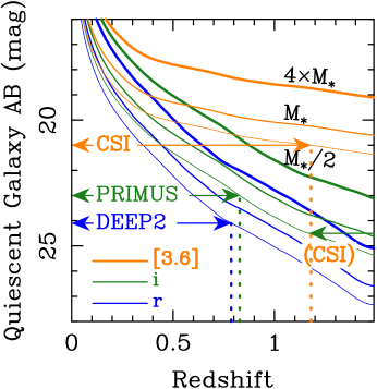
Figure 1.— (left) Apparent magnitudes in $r$, $i$, and $3.6\mu$m as a function of redshift, for passively evolving stellar populations ($3\leq z_{f}\leq 6$) with stellar masses $5M^{*}$ and $M^{*}/2$ ($\log M^{*}\sim 10.85$ at $z\lesssim 1$; Drory et al., 2009). The magnitude limits for DEEP2 (Willmer et al., 2006) and PRIMUS (Coil et al., 2011) are drawn. Such optical flux limits only cover the most massive passively evolving systems or those galaxies with young unattenuated stellar populations, biasing galaxy samples at early times. The shallow dependence of the $3.6\mu$m magnitude on redshift yields a selection with significantly less bias against old systems. The effective optical limit of CSI, $i=24.5$ mag, is also shown. The dotted vertical lines show the redshifts below which the DEEP2, PRIMUS, and CSI samples are not biased against old galaxies with stellar masses $M=M*/2$.

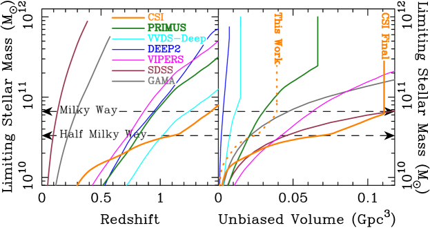
Figure 2.— (left) Limiting stellar mass of faint galaxy surveys by redshift. By using the IRAC $3.6\mu$m band, the CSI survey selection (the solid orange line) traces stellar mass more uniformly over most of the redshift range of the survey than samples selected in the optical. Our resulting sample is currently reaching $i=24.5$ mag (dashed green line), probing down to stellar masses equivalent to the present day Milky Way ($6.6\times 10^{10}M_{\odot}$; McMillan, 2011) out to $z=1.4$, almost order-of-magnitude lower than DEEP2, and half the present day Milky Way at $z=0.9$, a factor of two deeper than DEEP2 or PRIMUS. (right) Volumes probed with complete, unbiased samples for several redshift surveys as functions of limiting stellar mass. When the 15 deg² is completed, CSI’s volume (defined by the $3.6\mu$m- and $i$-band limits) will be more than an order of magnitude larger than DEEP2. The volume traced by the first 5.3 degs² (this paper) is shown by the dotted line.

2.2. The potential of an IRAC-selected survey

The integrated light of all but the youngest stellar populations are dominated by light from the stellar giant branch, cool stars whose light output peaks in the near-IR. It has long been recognized (e.g., Wright et al., 1994) that this results in a $1.6\mu$m “bump” – a peak in bolometric luminosity – for galaxies with a wide range of star formation histories. Indeed, as shown clearly in (for example) Figure 1 of Sorba & Sawicki (2010), this feature is nearly unchanging in Bruzual & Charlot (2003) models of stellar populations with mean ages 100 Myr $<\tau<$10 Gyr. Put in other terms, the near-IR mass-to-light ratio, M/L_1.6μm changes slowly for all but the youngest stellar populations.

The CSI Survey exploits the wide field and sensitivity of the Spitzer Space Telescope with the Infrared Array Camera (IRAC) to take advantage of this property of the integrated near-IR light from stellar populations in $z\sim 1$ galaxies. Combined with the insensitivity to internal and Galactic extinction, selection at $3.6\mu$m closely mirrors selection by stellar mass. Figure 1 directly compares the evolution of $3.6\mu$m magnitude with the optical $r$ and $i$ bands: the CSI selection wavelength has a dependence on redshift that is much shallower than surveys selected in the optical. What slope remains for the CSI selection function is an unavoidable k-correction: over the redshift range $0.7<z<1.5$, the center of the $3.6\mu$m IRAC band corresponds to restframe wavelengths of $2.1\mu m>\lambda_{c}>1.4\mu m$, straddling the $1.6\mu$m “bump” of the spectral energy distribution (SED) as it redshifts through the bandpass.

Thus massive galaxies exhibit a much flatter trend of observed magnitudes with redshift in the IR than in the optical, and this weaker dependence on galaxy mass afforded by $3.6\mu$m-selection of the sample is a key feature of the CSI Survey. Our goal has been to make a spectrophotometric survey to characterize galaxy populations and environments in an unbiased way down to a stellar mass of $M^{*}$ out to $z=1.5$, and down to a stellar mass of $M^{*}/2$ out to $z=1.2$. As can be read from Figure 1, a mass limit of $M^{*}$ corresponds to $r=26$ mag or $i=24.5$ mag at $z=1.4$, and $M^{*}/2$ corresponds to $r=26$ mag or $i=24.5$ mag at $z=1.2$. Our current spectroscopic reduction and analysis, described below, is reaching an effective optical limit of $i=24.5$ mag; brighter than this limit the CSI spectroscopic sample is correctably complete (though not necessarily uniformly complete; see §4.7 for more details).

Figure 2 (left) plots the limiting mass as a function of redshift for CSI (solid orange) and other redshift surveys. The depth of CSI in stellar mass is substantially less sensitive to redshift compared to the others due to the IRAC $3.6\mu$m selection, varying by a factor $\sim 3$ over $z=0.5-1.5$, compared to $1-2$ dex over the same redshift range for optically-selected surveys. Consequently, CSI samples a more uniform range of stellar masses over the full volume of the survey, and to a lookback time of 9 Gyr.

This critical point is illustrated in Figure 2 (right), plotting the depth in stellar mass against the volume probed with complete, unbiased samples. DEEP2, shown in violet (the line colors are the same as in the left), is limited in both area and mass depth. PRIMUS’s 9 degs² is limited in depth, and thus only probes an unbiased volume comparable to our first 5 degs². When CSI reaches its goal of 15 degs², the survey will cover an unbiased volume equal to the SDSS with similar depth in stellar mass. The large areas available from legacy Spitzer IRAC surveys — both wide and deep, and the freedom from foreground and internal extinction at this wavelength, allows the construction of uniformly deep, homogeneous photometric samples for spectroscopic follow-up.

CSI reaches factors of 2-6 deeper than DEEP2 in mass, over an area ultimately 8 times wider, and redshifts sufficiently accurate to characterize environments by directly identifying groups and clusters. With such data we aim to make the first group catalog at $z=1$ that is comparable in limiting mass and volume to SDSS, and thus enable detailed environmental characterizations of galaxies at a time when the universe was less than half its current age.

In this first paper, we describe the details of our data reduction and redshift fitting, redshifts for the first 45,284 galaxies in 5.3 degs² of the SWIRE-XMM field (Figure 3), and an initial characterization of the general galaxy populations in our stellar mass-limited sample.

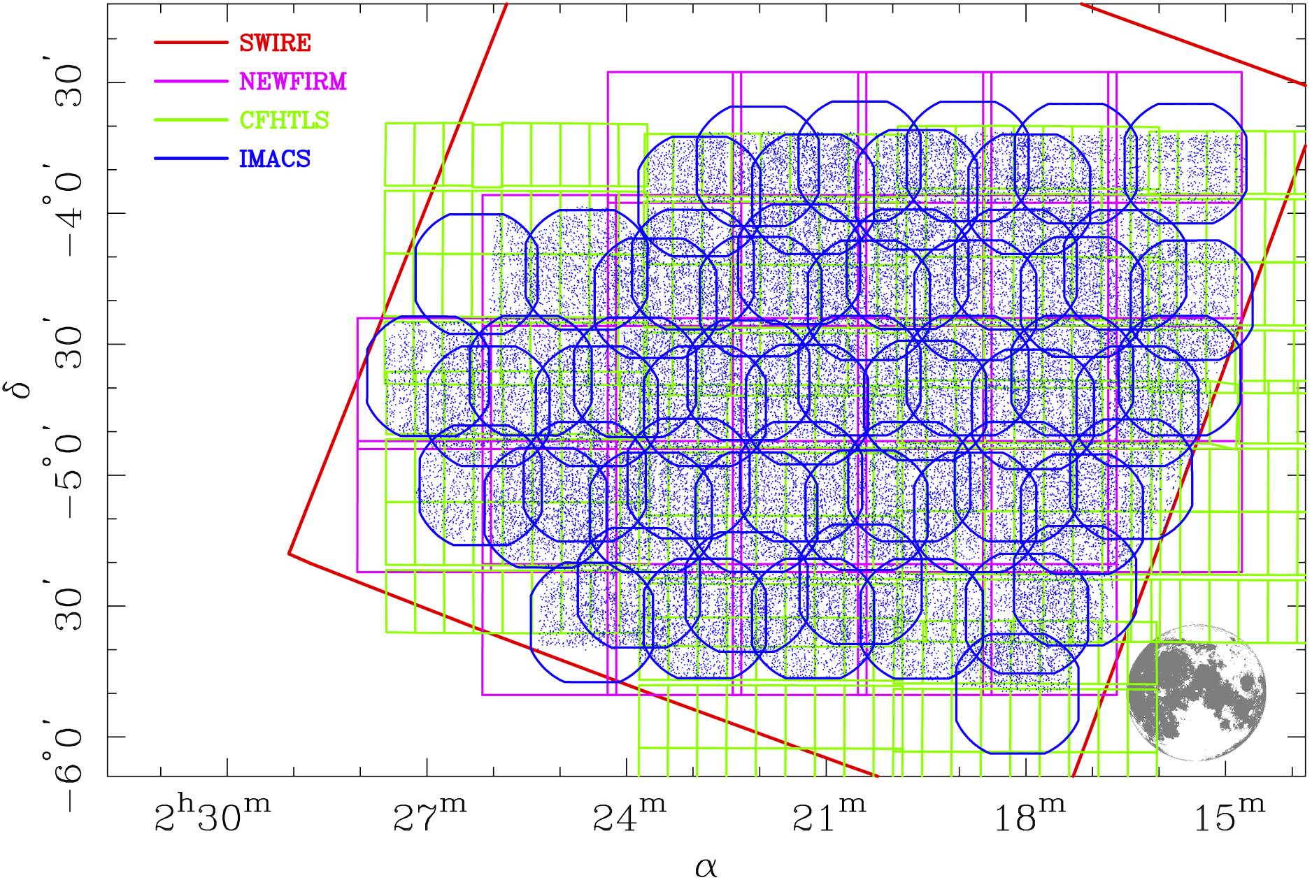
Figure 3.— A schematic of observations in the first 5 degs² of the SWIRE-XMM field studied by the Carnegie-Spitzer-IMACS survey. The SWIRE IRAC imaging field is outlined in red. The CFHTLS-W1 optical data reanalyzed by us is shown in green. The first set of NEWFIRM $J$ and $K_{s}$ observations are marked in violet. The positions of the IMACS slitmasks are outlined in blue, with the blue points marking the positions of the 46,600 galaxies with CSI redshifts. The field of view of IMACS is comparable to the size of the full moon, illustrated in the lower right.

3. Data

A project of this type and scope requires attention to detail and care in the processing and combination of a broad range of data from different sources. In this section we describe the imaging data and reductions that underpin the broadband flux measurements for the sample, both for the ultimate goal of fitting SEDs, but also for defining the selection criteria and incompleteness functions. Unless otherwise specified, all object detection was performed using SExtractor (Bertin & Arnouts, 1996).

3.1. Photometry

The SWIRE Legacy Survey (Lonsdale et al., 2003) observed several large fields with IRAC to a depth suitable for our survey. Three of these fields are accessible from southern telescopes, providing up to 23.8 deg² of coverage at $3.6\mu$m. Basic properties of the three fields are given in Table 1. Of these fields, $15.3$ deg² have supplemental optical imaging that is publicly available. Of the 9.1 degs² of IRAC imaging in the XMM-LSS field, 6.9 degs² is covered by the CFHT Legacy Survey W1 $ugriz$ imaging. In this section we discuss our analysis of the SWIRE XMM-LSS IRAC data, our reprocessing of the CFHTLSW1 $ugriz$ imaging and subsequent photometry of the $3.6\mu$m catalog, as well as our observations at $J$ and $K_{s}$ of the field using NEWFIRM (Autry et al., 2003) on the Mayall 4m telescope at Kitt Peak National Observatory.

3.1.1 Spitzer-IRAC Imaging

The SWIRE Legacy Survey was a program undertaken to trace galaxies by stellar mass back to $z=2$ (Lonsdale et al., 2003). We obtained the IRAC images of the XMM-LSS field from the archive at IPAC. The reductions and processing of these data were described by Surace et al. (2005). In order to minimize contamination of the object catalog by artifacts around stars, we configured SExtractor so as to ignore elliptical regions around bright stars. A ‘mexican hat’ convolution kernel was used for object detection, resulting in 585,159 objects in the $3.6\mu$m catalog of the XMM-LSS field. Fluxes were measured in a manner described by Surace et al. (2005). Down to our selection limit of $3.6_{AB}=21$ mag the $3.6\mu$m catalog contained 266,621 objects.

Table 1Basic Properties of the Southern SWIRE Fields Targeted by CSI

Field	SWIRE Area	SWIRE+Optical	Filters
	(degs2)	(degs2)
XMM-LSS	9.1	6.9	ugriz
ELAIS S1	6.9	3.6	BVRIz
CDFS	7.8	4.8	ugriz

3.1.2 The Optical Imaging

The CFHT Legacy Survey (Cuillandre & Bertin, 2006) targeted multiple fields using the one-degree MegaCam imager around the sky with a broad range of scientific goals. The “Wide” W1 field provided almost 7 deg² of overlapping $ugriz$ coverage in the SWIRE XMM-LSS field. Unfortunately, the processed images and catalogs available at Terapix were not entirely suitable for our purposes, owing to uncertain astrometry and inadequate defringing of the $i$ and $z$ data. To remedy this issue, we obtained the complete set of calibrated frames from the CFHT archive and processed the data using the following additional steps. We begin by constructing new fringe frames in $i$ and $z$ by medianing scaled exposures obtained within a single night. These were then rescaled and subtracted from the individual exposures. Some bright objects did bias these medians when the number of exposures was small (i.e. $N\hbox{${}_{<}\atop{{}^{\sim}}$}10$), leaving faint traces in the resulting fringe frames. In general, however, the greater sky uniformity after subtraction of these new fringe frames improved the depth of our resulting catalogs by $\sim 0.2$ to $0.5$ mag compared to the Terapix catalogs. We constructed sky frames as well for the $u,g$, and $r$ bands using a similar methodology, though not restricting the construction to data collected within single nights.

New astrometric solutions were derived for each exposure using the IRAC catalog as a set of deep astrometric standards. Cubic solutions for each chip were derived with a typical RMS scatter of 0^′′.15. For those regions of the MegaCam images that did not overlap the SWIRE data, we supplemented the catalog with the 2MASS point source catalog (Skrutskie et al., 2006), in order to prevent the solutions from diverging at the edges of the IRAC field.

Using these new astrometric solutions, and the photometric solutions from the headers of the individual frames, we constructed cosmic-ray-cleaned image stacks with 0^′′.185 pixels, 30 arcmin on a side and evenly spaced. These smaller images were more easily managed than the larger image formats provided by Terapix, which allowed us to distribute the image analysis and photometry tasks over multiple processors. The zeropoints were checked by comparing the photometry of moderately bright objects with the data in the catalogs from Terapix and we found systematic offsets less than $\pm 0.03$ mag in every case. Object catalogs were generated using SExtractor, and these were matched to the IRAC catalog with a tolerance of 1^′′.5 arcsec, with the goal of using the optical image characteristics to aid in star/galaxy separation, and to determine which IRAC-selected objects have centroids with optical centers falling far from the defined slit positions.

3.1.3 The Near-IR Imaging

NEWFIRM (Autry et al., 2003) is a wide-field ($27^{\prime}\times 27^{\prime}$) near-IR camera deployed by NOAO at the Mayall 4m at Kitt Peak from 2007 to early 2010. During the fall semesters we imaged the XMM-LSS field in $J$ and $K_{s}$. Typical exposure times were 70 min/pixel in $J$ and 32 min/pixel in $K_{s}$. The seeing ranged between $0.8-1.4$ arcsec (FWHM).

The data were processed using a fully automated, custom pipeline, written as a prototype for a wide-field imager being deployed at Magellan. The basic steps in the reduction were: (1) subtraction of the dark current; (2) correction for nonlinearity; (3) division by a flat-field; (4) masking of known bad pixels; (5) construction of first-pass sky frames; (6) derivation of image shifts, in arcsec, on the sky; (7) stacking of the first-pass sky-subtracted frames; (8) generation of a deep object catalog; (9) construction of object and persistence masks for second-pass sky estimation; (10) temporary interpolation over objects, persistence, and bad pixels for each frame; (11) constructing bivariate wavelet transforms of these masked frames; (12) fitting the time variation of the wavelet transforms of the sky using shorter frequencies for larger spatial scales; (13) reconstruction of model sky frames by inverting the temporally smoothed wavelet transforms; (14) subtraction of the model sky frames; (15) re-derivation of image shifts, in arcsec, on the sky; (16) final stacking of the sky-subtracted frames, including the generation of sigma and exposure maps; (17) identification of objects in the 2MASS point source catalog, restricted by 2MASS PSC quality flags; (18) application of rotation, translation, and scale to the camera distortion based on the 2MASS objects; and (19) calculation of image zero-points using the 2MASS objects.

Using the zeropoints of each image, we constructed image mosaics $30^{\prime}$ on a side centered at the locations of our $ugriz$ mosaics, but with 0^′′.4 pixels.

3.2. Aperture Photometry

Magnitudes in $ugrizJK_{s}$ were derived using aperture photometry within a range of circular apertures for the entire SWIRE catalog. Because the seeing varied with wavelength and pointing, we convolved the $z$-band image stacks (which had the best PSFs on average) with Gaussians to simulate the effects of poorer seeing in the $ugriJK_{s}$ data. The offsets in magnitude from the degraded $z$ images were applied as PSF-corrections to the $ugriJK_{s}$ aperture magnitudes. While the details of the PSF and potential blending are critical for small apertures and for modeling the profiles of the objects, our choice of fitting the SEDs to much larger-aperture ($D=4"$) magnitudes allows us to utilize a simple and economical approach to the PSF corrections — this choice was especially important given the enormous size of the object catalog. The choice of such a large aperture also reduces the systematic errors in matching the aperture magnitudes to the IRAC $3.6\mu$m fluxes.

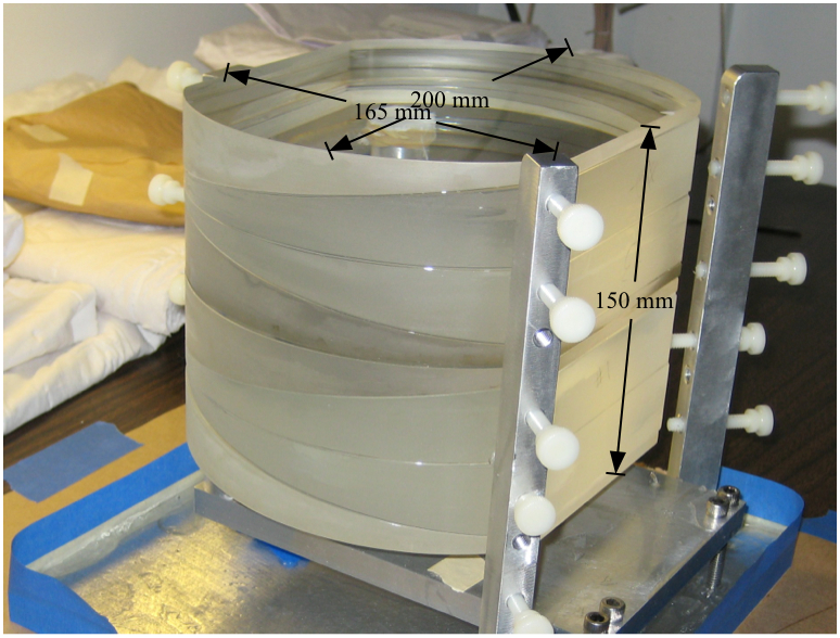
Figure 4.— Construction of the new “Uniform Dispersion Prism,” built for CSI. Dr. S. Shectman designed the UDP to have a resolution of $R\sim 25$ from 7500Å to 1$\mu$m. The eight layers are made from thin prisms of S-FPL51 and N-KZFS2, to make a stack of glass 150 mm thick. This prism has a resolution with a mild dependence on wavelength (see Figure 5) compared to the first prism deployed in IMACS (see Coil et al., 2011).

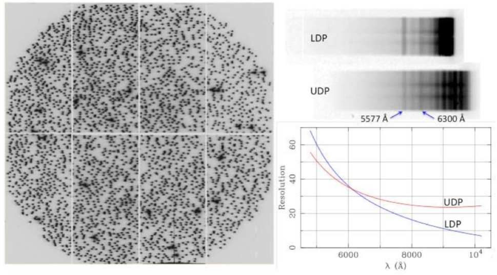
Figure 5.— (Figure reproduced from Dressler et al., 2011) (left) Multi-slit mask designed for use with the Low Dispersion Prism. (top right) Example LDP spectrum — nod & shuffle (Glazebrook & Bland-Hawthorn, 2001) produces doubled object and sky spectra. Night sky lines [O I]5577Å and [O I]6300Å are marked. Below the LDP spectrum is one obtained with the UDP, with its more uniform dispersion (bottom right). The resulting difference in resolution is shown in the bottom right. The resolution provided by the new Uniform Dispersion Prism, designed for CSI, provides an improved ability to trace the 4000Å break and [OII]3727Å to $z=1.4$ when coupled with IMACS’s red sensitive E2v detectors.

3.3. Spectroscopy

While the concept of using a low-dispersion prism for galaxy evolution has origins in PRIMUS, the infrastructure and background work for CSI’s observing strategy and data reduction was largely developed during the first author’s participation in the study of the $z=0.83$ cluster RXJ0152–13 and the intervening field (Patel et al., 2009a, b, 2011, 2012). Between 2008 and 2009 the SWIRE XMM field was targeted in 31 multislit mask exposures with the IMACS f/2 camera configuration and the Low Dispersion Prism (LDP) designed by S. Burles for the PRIMUS redshift survey (Coil et al., 2011). In 2010 we observed 29 SWIRE XMM masks using an innovative eight-layer disperser called the Uniform Dispersion Prism (UDP, see Figure 4). Although both of these dispersers produce spectra with median resolutions of $\lambda/\Delta\lambda\sim 30$, the dispersion curve of the UDP is much flatter, providing significantly higher resolution than the LDP out to $1\mu$m, at the expense of marginally lower resolution in the blue compared to the LDP (Figure 5).

Previous work by the PI on a similar program had obtained adequate $S/N$ ratios with exposure times of 3 hours down to $z^{\prime}=23.3$ mag using less sensitive SITe detectors (Patel et al., 2009a, b, 2011, 2012). Significantly more sensitive e2v detectors were installed in IMACS, thanks to support from the NSF’s TSIP program (see Dressler et al. 2011); these CCDs boosted the throughput of the instrument by factors of 2-3 in the far red. We observed with these detectors using the Nod and Shuffle mode of IMACS (see Glazebrook & Bland-Hawthorn, 2001), and accumulated exposure times of 2h per galaxy for more than 90% of the sample, using individual integrations with durations of 30 min (15 min per position). Typical slit lengths were 5 arcsec, with slit widths of 1 arcsec. The positions of the slit masks are shown in Figure 3. No blocking filter was necessary, as all of the light dispersed by prisms stays within a single order.

Spectrophotometric standards were obtained during most observing runs, with a consistency of 5% from run-to-run. Helium calibration lamps illuminating the deployable flat-field screen were taken approximately every hour (i.e., every other science exposure). In this section we describe the basic steps involved in reducing the multislit prism data using the custom pipeline that had been written for the earlier cluster programs (e.g. Patel et al., 2009a, b, 2011).

3.3.1 Wavelength Calibration

Two critical aspects of the reduction of LDP and UDP data involve mapping wavelengths on the detector, and transposing between sky coordinates of objects and CCD coordinates. The small number of He lamp lines are insufficient for determining accurate wavelength solutions in individual slitlets, so we derive global wavelength mappings over an entire CCD using all of the slitlets simultaneously. Thus, lines in a single spectrum that may be corrupted by bad columns or pixels will not affect the solution for that slitlet, as the $\sim 3000$ helium lines over a CCD frame constrain the fit.

The following are the basic, automated steps we have implemented in our pipeline:

• Derive mapping of sky coordinates to CCD coordinates using an image of the slitmask;

• Identify lines and fit 2D wavelength solutions using isolated helium lamp exposures on a chip-by-chip basis;

• Refit new centroids for blended helium lines using nonlinear simultaneous Gaussian fitting on a slit-by-slit basis;

• Fit for improved mapping of 2D wavelength solutions;

• Shift the wavelength maps using 2-3 night sky emission lines (e.g., [O I] 5577Å, Na 5890Å, [O I] 6300Å);

We start with a distortion map for the camera, defined from previous exposures of the field around the globular cluster Palomar 5, to compute the approximate mapping of sky coordinates to CCD coordinates for the objects in the multislit mask. SExtractor is run on a direct image of the slit mask and a simple pattern analysis matches up the predicted positions of the slits and the measured positions of the slits to create an adjusted mapping of sky coordinates to CCD coordinates.

With a theoretical dispersion curve for the prism, we generate a trivariate mapping of sky coordinates to CCD coordinates that is wavelength dependent. SExtractor is run on a helium comparison lamp image and the resulting catalog of the 3,000 to 4,000 helium lines is pattern-matched to the predicted positions of 8 unblended helium lines (out of the 11 lines in our line list). New wavelength mappings are solved for as the order of the fit is gradually increased. The nearly final solutions generated at this stage are first order rescalings of the theoretical dispersion, with coefficients that are cubic polynomials of the sky coordinates. The typical RMS at this stage is 0.3-0.4 pixels. With these solutions, we can now generate predicted positions for the complete helium line list and fit Gaussian profiles to the full line list for each slit. Within each slit, the Gaussians are fit simultaneously, providing accurate positions for both the unblended and blended helium lines. Using these new positions for the helium lines in CCD coordinates, we derive through iteration, the trivariate mapping between CCD coordinates and both wavelength and sky positions, with a typical final RMS scatter of 0.25 pixels. For LDP data this scatter corresponds to $\sim 50\,$Å at $9000\,$Å, or $\delta z\sim 0.005$. This large uncertainty in the wavelength calibration in the far red for the LDP is due to the fact that its dispersion reaches $\sim 200\,$Å/pixel at $9000\,$Å; the scatter of $\sim 50\,$Å introduces a 25% uncertainty in $\Delta\lambda$ at such wavelengths when computing the flux calibration. Because the resolution with the UDP is $3\times$ higher at these red wavelengths, this additional source of uncertainty is negligible for those data.

The final step involves cross-correlating simulated night sky emission lines ([OI]5577 Å, Na I 5890 Å, and [OI]6300 Å) placed at their predicted positions with the spectra in the science frames, on a slit-by-slit basis. The median offset in both $x$ and $y$ is then applied to the wavelength mappings found from the nearest helium lamp exposure.

3.3.2 Extracting Spectra

Due to the unique nature of these prism data, the science frames must also be processed in a nonstandard fashion using custom written routines. We take particular care in the extraction of spectra because of the small number of pixels covered by each object, the faint optical limits we expect to probe, and the proximity of the objects to slit ends where residual sky counts can bias simple extraction algorithms.

As can be seen in Figure 5 (top right), each object is exposed twice per readout. In our implementation of nod & shuffle, the object positions are shifted by 1.6 arcsec between the two spectra, A and B. Due to the fairly rapid timescale of the nodding (typically 60s), the sky backgrounds in the A and B exposures are functionally identical, and the subtraction of the A and B two-dimensional spectra from each other should leave only the object remaining. However, while nod & shuffle does provide excellent sky subtraction, the galaxy spectra themselves still must be divided by a flat-field. Flat-fielding data from nod & shuffle is also complicated by the fact that the A and B spectra were both exposed on identical detector pixels. Thus the pixels in the flat-field defined by the position of the A spectrum should be used to flatten both the A and B spectra. To summarize the first two steps of our reductions, first subtract 2D spectrum A from 2D spectrum B, and B from A. Next, divide the A-B spectrum and the B-A spectrum by those pixels in the (normalized) flat-field that were covered by spectrum A.

A first attempt to extract 1D spectra for every object in an exposure involves a simple form of optimal extraction (Horne, 1986), in which each object is assumed to have a Gaussian spatial profile. The centroid of the Gaussian is defined as a low-order polynomial of wavelength, and this polynomial defines the initial trace of the object. The second moment of the Gaussian is also computed as a low-order polynomial function of wavelength. Then a rough 1D spectrum for a given object can be obtained using this Gaussian approximation for the spatial profile in a manner similar to Horne (1986) but we opt to solve for the 1D spectrum in a least-squares sense, representing it as a b-spline (Dierckx, 1993), and allowing us to downweight bad pixels, cosmic-rays, or other discrepant data. With this approximate spectrum, we solve for new parameters of the spatial profile, including up to 4 Hermite moments (10 for spectrophotometric flux standards), with each of these moments defined as low-order polynomial functions of wavelength. The wavelength binning of the b-spline is defined by the wavelength solution for each slitlet.

When these spatial profiles and object moments have been derived for all eight CCDs of a given exposure, we analyze the differences between the predicted and measured object positions. These deviations are well described by a linear function of coordinates in the slitmask, largely reflecting the small misalignments of the mask that occurred when the observations were taken. We use this new linear function to fix the object positions, re-compute spatial profiles, and re-extract 1D spectra for each object in each exposure.

After deriving the traces and Gauss-Hermite moments of all the objects in all the exposures of a given slit mask, we perform a final optimal extraction using all of the exposures of a mask simultaneously. This procedure allows us to better flag (and ignore) cosmic-rays and other bad pixels, and to use the improved 1D spectrum of each object to further refine the spatial profiles and object positions. In this final extraction that combines all of the exposures, we incorporate the sensitivity function from our flux-calibration and produce spectra in physical units. Pixels, now all converted to flux units, are weighted according to the inverse of the expected noise and bad columns and pixels flagged as discrepant are given zero weight. Iteration allows us to flag and reject most cosmic rays, and to also re-weight the pixels using the “least-power” M-estimator (see below) in an effort to discount the noise estimates initially derived from the data frames. Blindly using noise that has been estimated from the original frames can lead to subtle, small biases in the resulting spectra; the iterative re-weighting helps mitigate the issue. The process performs an optimal extraction that yields a single 1D spectrum that matches all the data in a least-squares sense. While the exposure times are fairly uniform, the sky noise can vary greatly from exposure to exposure, especially as one approaches twilight or nearer to the moon. Given the small differences between the wavelength solutions of the exposures, we sample the one-dimensional b-spline representation of the spectrum at a fixed set of wavelengths, defined by the dispersion of the prism at the center of the field. This fixed grid greatly simplifies the construction of templates for fitting the SEDs.

Spectra for objects repeatedly observed in overlapping slitmasks were not combined at this stage, but kept separate — for this paper — so that we could better assess data quality and empirically estimate our redshift precision. Approximately 18% of the galaxies were repeated; we discuss these below in the context of the redshifts and their uncertainties. Approximately 20% of the objects observed with the LDP were also reobserved with the UDP.

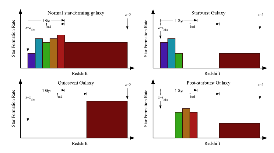
Figure 6.— Cartoon star formation histories for four representative galaxy types. Because optical passbands provide poor leverage on star formation histories earlier than 1 Gyr prior to the epoch of observations, we have reduced the complexity of galaxy star formation histories to nonnegative combinations of discrete components such as those illustrated in these cartoons. For our purposes, each galaxy is modeled with six age-related components, as described in the text, with the oldest component starting at $z=5$ and continuing down to some time $t_{end}$ prior to the epoch of observation. Five younger, discrete components of duration 200 Myr allow for the broad possible range of complex histories in a galaxy’s recent past. Each of these six components is quadrupled, with four different levels of extinction, $A_{V}\in\{0,0.5,1,2\}$ mag, leading to a total of 24 stellar components with non-negative contributions to the stellar mass of a galaxy. With redshift, metallicity, and $t_{end}$ as our gridded parameters, there are 24 stellar coefficients at each location in the grid. By abstracting star formation histories in this way, we have retained the essential information content of on-going star formation, intermediate-age populations, and an old, underlying stellar population.

3.3.3 Spectrophotometric Flux Calibration

Accurate flux calibration is a critical component of the survey because spectral slopes provide additional information to constrain galaxy redshifts. For CSI we choose bright hydrogen white dwarf standard stars with deep, broad Balmer lines that can be detected with the LDP/UDP. When taking a standard star spectrum, we place it in the center of an alignment star box on one of our slitmasks to ensure we are capturing essentially all of the star’s flux. Deep Balmer lines are thus required since they allow us to refine the wavelength calibrations for the stars when they are not accurately centered in the boxes.

The processing of standard star exposures is similar to that described above for the science exposures, with the following modifications. In order to derive the sensitivity function, we must first compensate for the fact that the seeing in the standard star exposure leads to different resolution than one would obtain with a narrow slit. We make an assumption that the seeing was isotropic and that the Gauss-Hermite parameterization of the spatial profile is a valid descriptor of the seeing profile in the dispersion direction. Using this profile as a kernel, we deconvolve the extracted spectrum using an implementation of CLEAN (Högbom, 1974), convolving the result to a resolution equivalent to that defined by the science data (FWHM=4.5 pixels). The wavelength calibration of the alignment star box is calculated with the trivariate wavelength solution of a helium lamp exposure obtained immediately after the standard star, with an additional correction from the measured positions of the star’s Balmer lines.

Due to time and weather constraints, spectrophotometric flux standards were not obtained during every night, but the excellent run-to-run repeatability of the relative flux calibration from 8500 Å to 4500 Å for the LDP (and from 9000 Å to 4500 Å for the UDP), of approximately $\pm 5\%$ allows us to use flux standards obtained on different nights or during different runs. We correct for slit losses, aperture corrections, and other such systematics as part of our SED fitting procedures, discussed in the next section.

4. SED Fitting

With broadband photometry and spectra in hand, a suitable library of template spectra can now be employed to estimate spectrophotometric redshifts. In this section we describe the basis functions in our templates, implement a generalized maximum likelihood method and estimate confidence limits for the redshifts of each galaxy along with several other parameters and properties.

Here we discuss the construction of the templates, using several continuum components, each derived from the Maraston (2005) models. The Kroupa (2001) initial mass function (IMF) was used, resulting in a median offset from “diet” Salpeter IMF (Bell & de Jong 2001) of 0.04 dex for SSP ages up to about 9 Gyr.

4.1. Ingredients

Ideally, a set of spectral templates should not only span the redshifts probed by a survey, but also encompass the potential range of optical and near-IR properties of galaxies over those epochs. Satisfying this latter constraint cannot be done a priori as it is one of the chief goals of the project. However, models of evolving stellar populations have been used for modeling low-dispersion prism data for the purpose of recovering redshifts to $z\sim 1$ (see Patel, 2010). Our method for CSI echoes that approach, and we describe it here.

Our templates are constructed as the superposition of several continuum components and multiple emission lines. The stellar population bases were derived from the Maraston (2005) models, using the Kroupa (2001) initial mass function (IMF). In building our templates we exploit the well known fact that for times $\tau\hbox{${}_{>}\atop{{}^{\sim}}$}1$ Gyr after the cessation of star formation, optical data no longer provide significant leverage on a galaxy’s prior star formation history (Tinsley, 1972). We adopt a simple set of stellar population basis functions: these components are sensitive to different timescales of a galaxy’s star formation history; in combination, they reproduce the broad range of SED properties seen in normal galaxies.

The first base component is a constant star formation model with a starting epoch of $z_{f}=5$. The time at which star formation ceases for this component is a free parameter in our analysis, a grid of values ranging from $10^{9}$ yr to $10^{10}$ yr prior to the redshift of observation (capped at $z=5$), whose values are spaced logarithmically with an interval of 0.10 dex. The metallicity of this base population is also gridded with values ranging from [Z/H]$=-1.2$ to [Z/H]$=0.6$, with an interval of 0.2 dex. Redshift is the final gridded parameter, ranging from $z=0.005$ to $z=2.0$ at intervals of $\Delta z=0.005$. Superimposed on the base population are up to five piecewise constant SFR populations that formed in 200 Myr intervals centered on lookback times of $t=1,3,5,7,9\times 10^{8}$ yr, with the same metallicity as that of the base. Four cartoon star formation histories built out of such components are schematized in Figure 6. The SEDs of each of these stellar components are redshifted, convolved to the wavelength-dependent resolution of the instrument, and sampled at the wavelengths appropriate for the galaxy spectra. Lastly, extinctions of $A_{V}\in\{0.0,0.5,1.0,2.0\}$ mag are applied to each component in an effort to reproduce the effects of complex dust distributions that are not well modeled by simple screen models.

In addition to the continuum components, we include several emission line components: (1) a single unresolved Gaussian emission line for [OII]3727 Å, (2) a blend of three Gaussians at [OIII]5007 Å, [OIII]4959 Å, and H$\beta 4861$ Å, with ratios of $1:1/3:1/10$, to broadly mimic the typical line ratios seen in galaxies at these masses (e.g. Kauffmann et al., 2004), (3) a Gaussian for H$\alpha 6563$ Å, and (4) an unresolved emission line for MgI2799 Å. Because of the increasing uncertainties in the flux calibration of LDP data beyond 8000 Å, no emission lines were allowed beyond that point in those fits. Given the higher quality of the UDP data in the far red, we extended this limit to 9000 Å in fitting UDP data, with the exception of [OII]3727 Å, which we accepted to 9400Å. These restrictions do not greatly affect the redshifts that are measured, but they do have some impact on the fit to the red continua of low redshift galaxies. Note that the widths of the Gaussian profiles are fixed to that defined by the spectral resolution.

Thus there are in total 24 stellar continuum components and 4 emission line components, each redshifted, convolved to the wavelength-dependent resolution of the instrument, and sampled at the wavelengths appropriate for the galaxy spectra. The broadband magnitudes of each component are computed using the filter transmission and detector QE curves of the respective imaging instruments.

4.2. Fixing the Flux Calibration

Before solving for the 28 coefficients at every location in the three-dimensional grid of redshift, metallicity, and termination time, we perform a step that solves for wavelength-dependent slit losses and aperture corrections, so that the IMACS spectrum and broadband photometry can be fit together as a single SED. This rescaling of each IMACS spectrum is derived using the broadband $griz$ photometry from the 4 arcsec diameter apertures. Performing this task on a galaxy-by-galaxy basis can be done accurately and robustly when the $S/N$ ratio of the photometry exceeds that of the spectroscopy, such as was done with deep SuprimeCAM data in Patel (2010). But in CSI, the CFHTLS-W1 data has a 5-$\sigma$ depth of $i\sim 24.5$ mag, and fitting for a separate wavelength dependence for each galaxy is not robust. Therefore we use the bright, red galaxies observed in a given mask to define a simple polynomial dependence for such slit losses and aperture corrections. The procedure is as follows: (1) construct a reduced set of templates, (2) fit these templates to the broadband fluxes of the bright, red galaxies, (3) derive rough photometric redshifts, (4) use these best-fit photometric templates to construct template prism spectra, and (5) ratio these prism templates with the observed prism spectra and fit low order polynomials. The resulting function is used for the wavelength dependence of the aperture corrections/slit losses for all objects within a given mask, allowing for a simple scaling of this polynomial for every galaxy to match the prism spectra with the broad-band photometry. At low redshift the adoption of a single polynomial to fix the flux calibration for an entire mask breaks down for large galaxies, contributing to some incompleteness at bright magnitudes. No significant correlations of the residuals from this fitting procedure are seen with respect to the positions of objects on the slit mask.

4.3. Fitting for the Galaxy Components

Standard least-squares and $\chi^{2}$ minimization techniques are susceptible to bad data points and outliers, for example, from a few residual cosmic rays or unidentified bad pixels, especially given the small number of usable pixels in each spectrum ($\sim 150$). We opted to perform an iteratively reweighted non-negative least squares fit for the template coefficients at each location in the grid, using the weight function of Huber’s M-estimator (Huber, 1981; Zhang, 1997). Doing so is equivalent to minimizing Huber’s M-estimator itself, given as $L_{Huber}$, with the associated weight function $W_{Huber}$:

$$L_{Huber}(x)= \begin{cases}L_{2}(x)&\text{if $|x|\leq k$}\\ k(|x|-k/2)&\text{if $|x|\geq k$}\end{cases}$$ (1)

$$L_{2}(x)= x^{2}/2$$ (2)

$$W_{Huber}(x)= \begin{cases}1&\text{if $|x|\leq k$}\\ k/x&\text{if $|x|\geq k$}\end{cases}$$ (3)

where $k=1.345$. Near the optimum location, points retain the behavior of $L_{2}=x^{2}/2$ (i.e. least squares) while outside points retain the behavior of $L_{1}=|x|$ (i.e. minimum absolute deviation), leading to an estimator that is robust against outliers but sensitive to the details of the distribution close to the optimum location. In three iterations the routine effectively minimized this M-estimator. By minimizing $L_{Huber}$, instead of the $L_{2}$ M-estimator, the fitting produces a set of coefficients that are robust against outliers and contaminated data, so long as the fraction of bad pixels is $\hbox{${}_{<}\atop{{}^{\sim}}$}25\%$.

Using the rescaled IMACS spectra and the $ugrizJK_{s}$ photometry, we solve for the template coefficients using iteratively reweighted non-negative least squares. The coefficients for each galaxy are stored, as well as several M-estimators for each grid location, for use in the final likelihood analysis (described below).

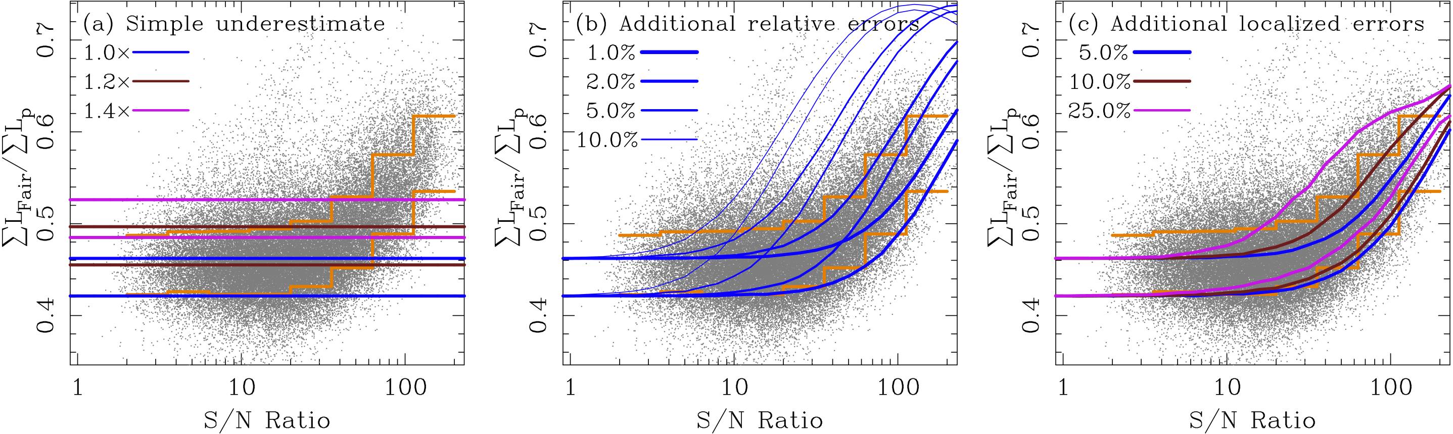
Figure 7.— Ratio of M-estimators $L_{Fair}$ and $L_{p}$ (see text) vs signal-to-noise ratio of the IMACS spectra (gray points). Orange lines show the 16th and 84th percentiles of the CSI data in bins of $S/N$. (a) Simple models where the true noise is $1\times$, $1.4\times$, and $2.0\times$ that used when performing a fit. These models show that are low and moderate $S/N$ ratios the CSI noise estimates have not been significantly under-estimated, but at high $S/N$ ratios there are additional sources of flux errors. For each model family we show a pair of lines to illustrate the 16th and 84th percentiles of the distributions. (b) Simple models are shown with additional (Gaussian) noise added at levels of 1%, 2%, 5%, and 10% of an object’s flux, proceeding from thick to thin. The curves mimic relative sources of random error such as simple flat-fielding uncertainties. The 16th and 84th percentiles are shown. (c) Models with a 1% “flat-fielding error” and added (Gaussian) noise contaminating 5 pixels per spectrum at levels of 3% (green), 12% (blue), and 40% (violet). Pairs of lines, again, show the 16th and 84th percentiles. Taken together, these models imply that the CSI spectra are largely consistent with $\sim 1\%$ flat-fielding or other relative errors and additional, localized sources of noise. In other words, residuals from the SED fitting show that the noise in the spectra is indeed non-Gaussian.

4.4. Likelihood Analysis

Each location in the three-dimensional grid of redshift, metallicity, and the termination of star-formation for the base ‘constant-star-formation’ model has a dozen coefficients, as well as goodness of fit metrics. With these grids of population coefficients and M-estimators, confidence limits on all of the gridded parameters and derived properties, such as total masses, stellar masses, restframe colors, were calculated using a likelihood function

$$\begin{split}d\mathcal{L}=&dzd\log t_{end}d[Z/H]P(z,\log t_{end},[Z/H])\times\\ &\exp\bigl{[}{-\sum L_{Huber}(x|z,\log t_{end},[Z/H])}\bigr{]}\end{split}$$ (4)

where $P$ is the defined set of priors at a given redshift, termination time, and metallicity, and $x$ is the set of observations over which the M-estimator is summed. In our likelihood analysis we found that using Huber’s M-estimator gave results that were most robust to bad pixels without biasing the contributions of emission lines, though others, for example, “least-power” or “Fair” (see, e.g., Zhang, 1997), were also very effective. We caution against using M-estimators that are insufficiently concave, as pixels “contaminated” by real (but narrow) features such as unresolved emission lines are attributed less weight than continuum pixels (by definition). With these three dimensional likelihood functions, we have 24 SFH + 4 emission line parameters at each location in the grid.

For every spectrum, we marginalize over redshift, stellar mass, rest frame colors, stellar population parameters as per the components in the SED fitting, and emission line luminosities, estimating 68%, 90% and 95% confidence intervals for every parameter and property. Several criteria are employed to define the sample that has successfully passed through the SED fitting, including sensible restframe colors and physically meaningful stellar masses. We also restrict the sample to the set of galaxies with formal 95% uncertainties in rest frame $M_{g}$ of $\Delta_{95}M_{g}<2.0$ mag (equivalent to $\sigma_{M_{g}}<0.5$ mag). The result is a relatively clean sample of 45,286 galaxies with a total of 55,490 spectra, over a field of 5.3 degs².

We will use these confidence limits, along with data quality measures derived from additional M-estimators, to identify a high quality sample in the next sections.

4.5. Using M-estimators to Probe Data Quality

Assessing the quality of any data involves more than the estimation of $S/N$ ratios and calculations of reduced $\chi^{2}$ — statistics that rest on simplistic or potentially unrealistic assumptions for the underlying sources of noise. In this section we investigate the distributions of residuals from the SED fitting using M-estimators and construct a new statistic to assess data quality. Because they display varying degrees of sensitivity to outlying data points, comparisons of M-estimators directly probe how well the errors in the flux measurements have been estimated. Because one’s measurement uncertainties underpin any likelihood analysis, confidence in one’s measurement errors translates directly to confidence in any confidence intervals. And while no simple combination of M-estimators will provide a complete description of the distribution and sources of bad data, the heuristic approach shown below provides important initial insights that we expect to push further as we complete the remainder of the survey.

We first assume that on average the residuals from the maximum likelihood analysis reflect the true distribution of flux errors. The magnitude of these residuals, normalized by our estimated measurement errors, probes both the extent to which uncertainties have been improperly estimated and the extent to which bad pixels contaminate the data. Recall that most likelihood analysis is of the form $\exp{(-L_{2})}$, with some limited analysis of $\chi^{2}$. However, such work can only provide insight so long as $[f_{model}(\lambda)-f_{observed}(\lambda)]/\sigma(\lambda)$ is drawn from a Gaussian distribution with a standard deviation of unity. M-estimators have been designed to mitigate against specific non-Gaussianities — long tails and sporadic spurious points — and such “best fit” solutions are significantly less biased by bad data. However, wholesale under- or over-estimation of measurement errors may remain an issue in one’s data, and different M-estimators will reflect this to varying degrees. Thus, ratios of M-estimators have the potential to become powerful tools for identifying galaxies in our sample that have been contaminated by spuriously bad pixels, have simply had their flux errors under-estimated due to poorly handled systematics, both intrinsic to the data or introduced in the reduction process, or have substantial systematic errors due to template mismatch or poor calibration (e.g. flat-fielding).

For this analysis we introduce the “Fair” and “Least-power” M-estimators (Zhang, 1997):

$$L_{Fair}(x)= c^{2}\bigl{[}\frac{|x|}{c}-\log(1+\frac{|x|}{c})\bigr{]}$$ (5)

$$L_{p}(x)= |x|^{1.2}/1.2$$ (6)

and use the ratio $\sum L_{Fair}/\sum L_{p}$ as a means to assess data quality. A higher ratio indicates that the formal errors have been underestimated. Since this ratio doesn’t include $\sum L_{Huber}$, which was optimized in our SED fitting, the ratio $\sum L_{Fair}/\sum L_{p}$ provides a relatively independent check on the data quality. This statistic represents a helpful moment of the distribution of residuals from the SED fitting in a way that captures the extent to which the noise was properly accounted for. After all, the noise estimates underpin the shape of $\mathcal{L}(z)$.

For a Gaussian distribution of residuals, with perfect estimates for the measurement uncertainties, the ratio $\sum L_{Fair}/\sum L_{p}$ converges to $\sim 0.44$. For a survey with many thousands of spectra with only 50 resolution elements, 68% of $\sum L_{Fair}/\sum L_{p}$ should fall between $0.42\lower 1.29167pt\hbox{$\scriptscriptstyle\;\buildrel<\over{\sim}\;$}\sum L_{Fair}/\sum L_{p}\lower 1.29167pt\hbox{$\scriptscriptstyle\;\buildrel<\over{\sim}\;$}0.46$. For non-Gaussian distributions the ratio increases. Therefore, a finding of $\langle\sum L_{Fair}/\sum L_{p}\rangle\gg 0.46$ for a set of data indicates that the noise estimates were underestimated — though one does not know if the elevation in noise was due to contamination by spurious data or to a simple underestimate of the Gaussian noise. But by using simple Monte Carlo experiments we calculate how this ratio is correlated with $S/N$ ratio under the assumption that a range of systematic measurement errors plague the data set. Comparing the resulting trends with what is seen in the CSI data, we can better understand how to divide the CSI sample according to a quantitative assessment of data quality. For this analysis we consider only the residuals from the fits to the spectra, ignoring the broadband photometric residuals.

Figure 7(a-c) shows $\sum L_{Fair}/\sum L_{p}$ plotted against $S/N$ for those objects that passed the initial SED fitting quality checks. Orange lines show the 16th and 84th percentiles of the data in bins of $S/N$ ratio. Several simple noise models are overlaid. In Figure 7(a) the blues lines mark the 16th and 84th percentiles one obtains with Gaussian noise that has been perfectly estimated. The maroon and violet lines represent ratios obtained when the noise is underestimated by factors of $1.2\times$ and $1.4\times$, respectively. The spectroscopic residuals from our SED fitting are not consistent with such simple underestimates of the errors in the IMACS spectra.

In Figure 7(b), we show models in which additional (Gaussian) noise is added at levels of 1%, 2%, 5%, and 10% of an object’s flux, with progressively thinner lines. These curves indicate that our data have additional sources of noise unaccounted for in our analysis that are typically at levels of a few percent or less. Such levels may result from errors in flat-fielding or from a general mismatch of templates, for example. However, the additional sources of noise need not be uniformly distributed within each spectrum. In Figure 7(c), we start with the 1% “flat-fielding” noise and contaminate 1 resolution element, with additional, localized noise at levels of 5%, 10%, and 25% of an object’s flux in those pixels.

While the permutations of such models may be infinite, the residuals in the CSI data are reasonably well described by some combination of the estimated noise due to the sky, object, and detector electronics, plus flat-fielding errors at levels of $\sim 1\%$, plus additional sources of bad pixels containing noise at levels of several percent. These trends should remind reader the combined sources of noise in the data are indeed non-Gaussian, justifying our use of M-estimators in this maximum likelihood analysis.

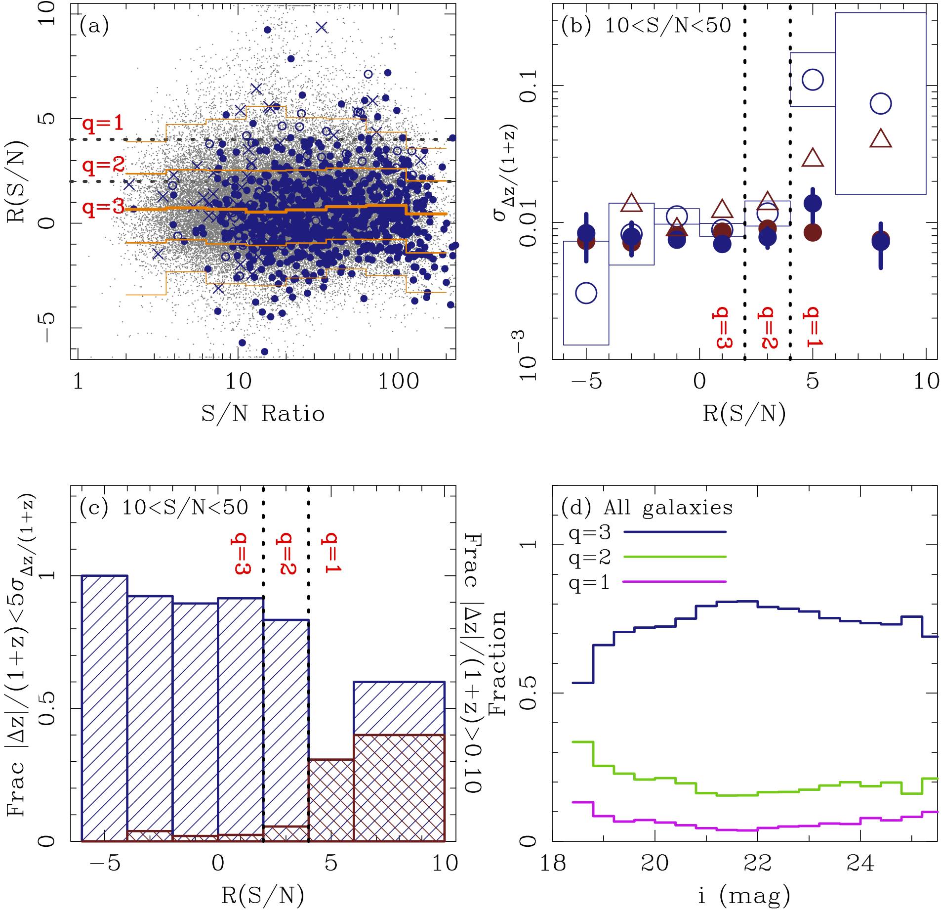
Figure 8.— (a) The ratio $\sum L_{Fair}/\sum L_{p}$, renormalized by the noise model shown by the blue lines in Figure 7(c), shown as a function of $S/N$ ratio. Large values of $R(S/N)$ reflect larger moments of the distributions in residuals from the SED fitting than expected from the estimated errors. (b) For galaxies with $10<S/N<50$, we plot the robust standard deviation in the fractional redshift errors of galaxies vs $R(S/N)$ using open circles, with the rectangles denoting the 1-$\sigma$ uncertainties. Filled blue circles mark the mean redshift uncertainty in each bin as derived from the CSI likelihood functions. Red triangles show the estimated redshift errors derived from those objects with repeat observations, while the filled red circles mark the mean redshift uncertainty derived from the CSI likelihood functions for those particular galaxies. Objects with $R(S/N)\lower 1.29167pt\hbox{$\scriptscriptstyle\;\buildrel>\over{\sim}\;$}4$, have significantly larger redshift errors than estimated from the likelihood functions, and thus earn the lowest quality flag, $q=1$. (c) The fraction of galaxies with redshift errors less than $5\sigma$ [see the blue points in b] are shown with blue hatched regions. The fraction of catastrophic failures ($>0.10$ in $|\Delta z|/(1+z)$) is shown in dark red. Objects with $R(S/N)\lower 1.29167pt\hbox{$\scriptscriptstyle\;\buildrel<\over{\sim}\;$}2$, have catastrophic failure rates of $<5\%$. These define the highest quality sample, $q=3$, in which $>90\%$ of these galaxies also have redshift errors $|\Delta z|/(1+z)<5\sigma_{\Delta z}/(1+z)$. Intermediate quality, $q=2$, is defined by $2<R(S/N)<4$. (d) We plot the fractions of galaxies with each quality flag as a function of $i$-band magnitude. The quality flags are not, per se, definitions with respect to absolute redshift uncertainty but definitions regarding the quality of the redshift uncertainties themselves.

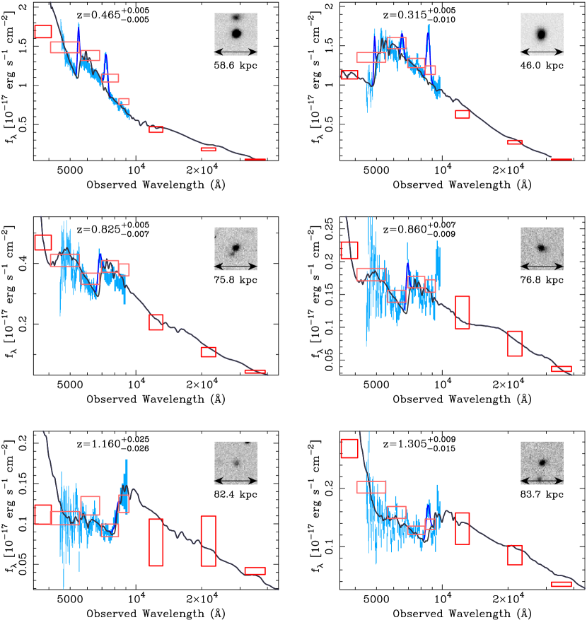
Figure 9.— Example SEDs for blue galaxies, along with their CSI redshifts and 95% confidence limits. The IMACS spectra are shown in cyan. The red boxes mark the broadband flux measurements in $ugrizJK_{s}[3.6]$, noting that the SED fitting was performed using $ugrizJK_{s}$. The best-fit stellar population models are shown with thick black lines. When the data require emission line components in the fit, these are shown using dark blue. Inset we show the CFHTLS $z$-band images of the galaxies. In particular, we note that for a number of these galaxies the broadband photometry alone would be insufficient to provide high quality redshift estimates. Low dispersion spectroscopy was key to isolating Balmer breaks and emission lines in blue galaxies, leading to very little dependence of redshift uncertainties on spectral type in CSI.

Figure 10.— Same as in Fig. 9 but for red galaxies in CSI. Note the structure in the SEDs traced by both the data and the models outside of the 4000Å break.

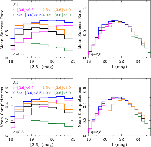
Figure 11.— (top) Average success rate as functions of $3.6\mu$m and $i$ magnitude, where success rate refers to the fraction of slitlets cut that led to high quality redshift measurements ($q\in\{2,3\}$). (bottom) The average completeness as functions of $3.6\mu$m and $i$ magnitude, where completeness is the fraction of galaxies above the $3.6\mu$m flux limit within the 5.3 degs² area that have CSI redshifts. At a given $3.6\mu$m flux, the completeness is a fairly strong function of color, such that it very nearly depends on $i$-band magnitude alone.

4.6. Defining Data Quality Flags

We now adopt the noise model shown in blue in Figure 7(c) as the baseline for defining spectroscopic data quality, since it effectively follows the lower boundary of the locus of points. We refer to the 50th percentile curve of this set of Monte Carlo simulations as $M(S/N)$, and use the 68% population interval, at fixed $S/N$, to define the significance of a deviation from $M(S/N)$:

$$R(S/N)=\log\bigl{[}\frac{\sum L_{Fair}}{M(S/N)\sum L_{p}}\bigr{]}/\sigma_{\log M(S/N)}$$ (7)

At a given $S/N$ ratio, galaxies that lie far above $M(S/N)$ either have problematic data or have severely underestimated flux uncertainties. $R(S/N)$ thus serves as a diagnostic of data quality based on the CSI data themselves, requiring no external redshift or spectral data.

Figure 8(a) plots $R(S/N)$ vs $S/N$ ratio. The small gray points are the same as in Figure 7. The orange lines trace the 2nd, 16th, 50th, 84th, and 98th percentiles. The large, blue points are galaxies with previously known spectroscopic redshifts. In this initial CSI sample, there are 710 galaxies with redshifts known from high resolution data. Roughly half of these can be found in the VVDS (Le Fevre et al., 2003), another $\sim 90$ from Cooper & Weiner (2013), and the remainder come from the UDS itself (Simpson et al., 2010; Akiyama et al., 2010; Smail et al., 2008). We have visually inspected and verified redshifts of the VIMOS spectra of galaxies common to the VVDS and CSI, in a few cases revising VVDS redshifts and quality flags. For VVDS objects flagged as ‘low quality’ (3 & 2), we were not able to verify all redshifts; we nevertheless include them here. We will return in §4.8 to a more in-depth comparison of redshift measurements once we have defined data quality flags.

In Figure 8(b) we use the open blue circles to plot the standard deviation of the fractional redshift errors in bins of $R(S/N)$, (using $\sigma=1.48\times$ MAD, or median absolute deviation; Beers et al., 1990), using bootstrapping to estimate the 1-$\sigma$ uncertainties marked by the rectangles. We restrict the sample to those galaxies with spectra having $10<S/N<50$, in order to avoid being biased by any underlying trends of $S/N$ ratio with $R(S/N)$. The blue filled circles show the mean fractional redshift uncertainty as derived from our confidence limits on the redshifts. Galaxies with $R(S/N)\lower 1.29167pt\hbox{$\scriptscriptstyle\;\buildrel>\over{\sim}\;$}4$ have significantly larger redshift errors than was estimated from our likelihood functions. For those galaxies with repeat measurements, we estimate their mean redshift errors and plot those with red triangles. Red filled circles indicate the expected mean redshift uncertainties for those galaxies and the repeat measurements reinforce our conclusion that objects with $R(S/N)>4$ show redshift errors significantly larger than the uncertainties derived from the likelihood analysis.

In Figure 8(c) the blue hatched region shows the fraction of galaxies with redshift errors less than 5-$\sigma$, where $\sigma$ is the mean estimated redshift error from the confidence limits (i.e. the blue points in b). In red , we show the fraction of galaxies with redshifts in error by more than $|\Delta z|>0.10\times(1+z)$. This “catastrophic failure” rate is $<5\%$ for galaxies with $R(S/N)\lower 1.29167pt\hbox{$\scriptscriptstyle\;\buildrel<\over{\sim}\;$}2$, and $<10\%$ for galaxies with $R(S/N)\lower 1.29167pt\hbox{$\scriptscriptstyle\;\buildrel<\over{\sim}\;$}4$. With this in mind, we define a “quality” parameter, $q$, based on $R(S/N)$ cuts.

The highest quality CSI data are those galaxies with $R(S/N)<2$ ($q=3$). For galaxies with $2<R(S/N)<4$ ($q=2$), the catastrophic failure rate remains low, at $5.5\%$. We therefore consider galaxies with $R(S/N)<4$ ($q=2-3$) as adequate for general scientific work. CSI data with $R(S/N)>4$ make up the low quality subset ($q=1$) of CSI. Note that while we restricted Figures 8(b) and 8(c) to those galaxies with $10<S/N<50$, the basic trends are consistent over both narrower and broader $S/N$ ranges.

Figure 8(d) shows the relative fractions of galaxies with each quality flag as functions of $i$-band magnitude. Given that the quality thresholds in $R(S/N)$ run nearly parallel to the orange lines in Figure 8(a), it is not surprising that the fraction of the sample with a given quality flag does not depend strongly on magnitude for galaxies fainter than $i=19$ mag. At bright optical magnitudes, the spectroscopic residuals become dominated by template mismatch (and even saturation in extreme cases). For the rest of the paper, we refer to the “highest quality” sample as the set of 36,481 galaxies with $q=3$, and the “high quality” sample as the set of 43,347 galaxies with $q\in\{2,3\}$. For the remainder of the paper, we ignore the 1937 galaxies with $q=1$.

Example data and SED fits illustrating the ability of CSI to trace spectral features over a broad range of redshifts and spectral types are shown in Figures 9 and 10.

4.7. Success Rates and Completeness

In a spectroscopic galaxy survey, the degree to which the population is sampled can be characterized by two quantities: the success rate (fraction of targeted galaxies for which usable spectra are obtained) and the completeness (fraction of the original photometric sample that is observed and usable spectra obtained). The former quantity is naturally folded into the latter, which also involves fundamental observational limitations (finite telescope time, slit collisions, and imperfect detectors, among others).

In most high resolution spectroscopy, the successful measurement of a redshift hinges on the (visual) identification of specific features, often prominent emission and/or absorption lines. To be considered a secure redshift in such surveys, multiple features typically must be seen. A program’s success rate, which can depend strongly on magnitude and/or color, is usually intertwined with the underlying distribution of galaxy redshifts and emission line luminosities; “successes” occur when these features fall within the spectroscopic window with sufficient S/N ratios to be reliably identified.

On the other hand, incompleteness in photometric redshift surveys depends on fits of template SEDs to flux measurements made over a (hopefully) wide baseline in wavelength. Specific narrow features are not required to fall within a particular window; rather, redshifts are largely constrained by broad breaks in galaxy SEDs. At low $S/N$ ratios the SED fitting can degrade, sometimes leading to larger uncertainties in the derived parameters (redshift, age, etc), and occasionally resulting in unphysical solutions. Artifacts like poorly handled bad pixels, cosmic rays, improper fringe correction, and blending may similarly cause the SED fitting to fail for some fraction of spectroscopic targets.

The Carnegie-Spitzer-IMACS Survey, with its combination of low-resolution spectroscopy and broadband photometry, does not depend on the presence of critical spectral features within the spectroscopic bandpass. Instead, the factors which contribute to incompleteness in CSI more closely resemble those that affect broadband photometric surveys. The presence of, e.g., strong [OII]3727Å can certainly lead to highly secure redshifts in some cases. However, the power of this survey comes with the ability to trace intermediate-width structure within the SEDs, such as the broad Ca H&K absorption, the G band, or even the structure around the MgII absorption at restframe 2800Å in older stellar populations.

Success for CSI therefore depends on the quality of the photometry and the extracted 1D spectra, which jointly constitute our SEDs. Having too low a S/N ratio in the IMACS spectra is usually an issue at magnitudes fainter than i=23.5, and at these flux levels the photometry is especially crucial. The portion of a spectrum used in the SED fitting is only about 140 pixels long, leaving them susceptible to bad CCD columns and artifacts at the ends of the short slitlets

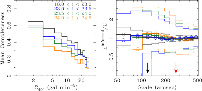
Figure 12.— (left) The mean completeness as a function of local source density computed on scales of $40\times 40$ arcsec, approximating the portion of our incompleteness arising from slit collisions. (right) The accuracy with which local galaxy counts are reproduced by our high-quality sample alone, when summing the inverse of the completeness as weights on individual galaxies. The thick lines indicate that, on average, there is no systematic bias in the local source densities inferred from the CSI redshift catalog down to $i=24.5$ mag, with a standard deviation of $0.1-0.3$ dex, depending on the scale over which galaxy number counts are estimated. Using the scaling relations for massive halos from Carlberg et al. (1997) and Carlberg et al. (2001), one infers that halos with masses $M_{vir}=5\times 10^{14}M_{\odot}$ and $M_{vir}=5\times 10^{13}M_{\odot}$ at $z=1$ have typical diameters of $\sim$ 4.5 arcmin (red arrow) and $\sim 2$ arcmin (black arrow), respectively. Based on these calculations We infer that slit collisions and other sources of incompleteness introduce no systematic errors in our accounting of the numbers of galaxies present in group-sized halos and larger.

In Figures 11 (top) and (bottom) we plot the CSI success rates and completeness as functions of $[3.6]$ and $i$-band magnitudes, also breaking down the sample into coarse bins of galaxy color. We model the completeness as a 2D function of both $3.6\mu$m magnitude and $i-[3.6]$ color, and for illustrative purposes Figure 11 shows the mean rates of success and completeness within broad color bins. We are thus able to estimate the incompleteness in the final sample given a galaxy’s magnitude, color, and local source density. Our peak success rate is 70% between $20<i<22.5$ mag, and at those magnitudes the completeness is about 50%. At $i=24$ mag the current pipeline produces a mean success rate of 40%, resulting in a mean completeness for CSI of 30%. Down to $i\sim 24.5$ mag the incompleteness is well-characterized and can be corrected; below this, the completeness corrections become more problematic (as does the CFHTLS photometry).

To first order, the success rate is simply a function of $i$-band magnitude. Notably, the distribution of estimated redshifts of the lower quality data ($q=1$) is not statistically different from the high quality sample except at faint magnitudes ($i>23.5$ mag). In any case, it is critical that our completeness corrections correctly model what was lost as functions of magnitude, color, and most importantly, local source density.

This last factor profoundly influences the completeness of spectroscopic surveys like CSI through slit collisions. To model this, we divided our sample into bins based on local source density. The footprint of a CSI spectrum is $\sim 200$ pixels wide, or 40 arcsec, by 10 arcsec (including both the A and B spectra). For every target and observed galaxy, we measure the local source density in $40\times 40$ arcsec ($4/9$ arcmin²) boxes. We then compute the mean completeness in bins of local source density, shown in Figure 12(left). This declining function illustrates the worsening effects of slit collisions at high projected source densities. We also have compared the bivariate ($[3.6]$, $i-[3.6]$) completeness functions in coarse bins of source density, but find no statistically significant variation. This consistency allows us to treat separately the decreasing completeness as a function of source density, and the joint effects of $i$-band magnitude and $i-[3.6]$ color.

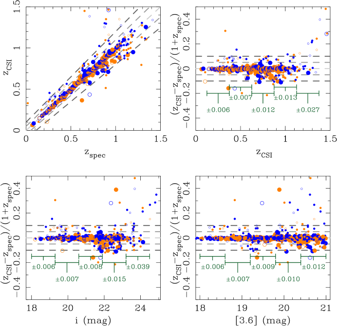
Figure 13.— (top left) Galaxies with high quality CSI redshifts ($q\in\{2,3\}$) plotted against redshifts in the VVDS and in the UDS from Cooper & Weiner (2013) with quality flags 3,4,5. Larger symbols indicate higher quality redshift flags from the high resolution datasets. The dashed lines mark the loci of $|\delta z/(1+z)|=0,0.05,0.10$ from lightest to darkest, respectively. In orange and blue we show those galaxies observed with the LDP and UDP respectively. (top right) Fraction redshift error vs. VVDS redshift. Numbers shown with bins along the x-axis show the $1\sigma$ estimate of the scatter, computed using $\sigma=1.48\times$ MAD (median absolute deviation; Beers et al., 1990). Overall agreement is excellent, with a median systematic bias of $\langle\delta z/(1+z)\rangle=-0.004$ and low scatter that is largely correlated with redshift and $i$-band magnitude, and less so with $3.6\mu$m magnitude. For the 85 galaxies with CSI redshifts $0.7<z<1.0$ and high quality VVDS redshifts (quality flags 4 & 5), 95% have redshift differences $\delta z/(1+z)<0.05$ and a $1\sigma$ scatter of $0.010$ in $\delta z/(1+z)$. The numbers of CSI measurements with redshift errors $|\delta z/(1+z)|>0.10$ and $>0.05$, and the number of CSI measurements within each bin, are given in Table 2.

We tested our density-dependent completeness corrections in order to verify that the effects of slit collisions do not systematically bias measurements of galaxy environment. Using those galaxies with CSI redshifts to infer the projected local source densities, we show the accuracy with which the intrinsic projected densities can be recovered in Figure 12(right). In the figure we plot the ratio of the inferred local source densities for galaxies in several $i$-band magnitude bins to true local densities of galaxies in those magnitude ranges. We plot the 16th, 50th, and 80th percentiles as dashed, solid, and dashed lines, showing the error in inferred local source density as a function of the linear scale over which the densities were computed. For comparison, the correlation of $R_{200}$ with $M_{vir}$ (e.g. Carlberg et al., 1997, 2001) implies circular diameters of $\sim$ 270 arcsec and $\sim 120$ arcsec for halos of mass $M_{vir}=5\times 10^{14}M_{\odot}$ and $M_{vir}=5\times 10^{13}M_{\odot}$, respectively, at $z=1$. The systematic bias in the recovered local source densities is less than 10% at all magnitudes and scales larger than $\sim 2$ arcmin.

The distribution of inferred to total densities is asymmetric on the shortest scales and at the faintest magnitudes; this is driven by small number statistics. Essentially, when the inferred source density is zero, there may be two reasons: the true source density may, in fact, be zero, or there may be one or two galaxies present that were simply missed by the slitmasks or rejected by our quality cuts. The combination of slit collisions and the dependence of the completeness on $i$-band flux imply an effective optical limit of $i\sim 24.5$ mag for environmental studies with CSI for scales down to $\sim 2$ arcmin. The 1-$\sigma$ confidence intervals also indicate that the inferred local densities of galaxies at a given magnitude have typical formal uncertainties of $\lower 1.29167pt\hbox{$\scriptscriptstyle\;\buildrel<\over{\sim}\;$}0.2$ dex. Thus, incompleteness, including the effects of slit collisions, add $\lower 1.29167pt\hbox{$\scriptscriptstyle\;\buildrel<\over{\sim}\;$}0.2$ dex to the uncertainty in, for example, group masses when estimated from counting up galaxies within radii $\lower 1.29167pt\hbox{$\scriptscriptstyle\;\buildrel>\over{\sim}\;$}2$ arcmin.

4.8. Redshift Uncertainties

We have three different methods at our disposal for evaluating the accuracy of CSI redshifts: (1) directly comparing our results with hundreds of optically-selected high-resolution spectroscopic redshifts from several sources; (2) deriving uncertainties using the large number of objects with repeat measurements; and (3) employing the Quadri & Williams (2010) pairwise velocity approach, in which galaxy groups and large scale structures mean that a significant fraction of galaxy pairs are physically associated, effectively providing repeat redshift measurements of cosmic structures. In the following, we apply these three metrics to our CSI data to robustly test the reliability of our redshifts (and their quoted uncertainties).

4.8.1 Direct Comparisons with High-Resolution Spectroscopic Redshifts

Figure 13 shows a direct comparison of previously published spectroscopic redshifts with those derived by our SED fitting. Figure 14 breaks this comparison down by CSI data quality. For the 227 high quality VVDS measurements that overlap our sample, 91% of the redshifts agree to within $\delta z/(1+z)<0.02$, with 96% within $\delta z/(1+z)<0.05$. The standard deviation for this subsample is $\sigma_{z}/(1+z)=0.007$ (using $\sigma=1.48\times$ MAD), with a bias of $\langle\Delta z/(1+z)\rangle=-0.004\pm 0.0005$ (standard error of the mean). For the 194 poorer quality VVDS measurements, we find a scatter of $\sigma_{z}/(1+z)=0.015$, with 88% agreeing to within $\delta z/(1+z)<0.05$, and a slightly larger bias of $\langle\Delta z/(1+z)\rangle=-0.005\pm 0.002$. This bias in the redshifts is roughly equivalent to half a pixel, suggesting that systematic errors in our wavelength calibrations may remain at that level. This offset is consistent with the small shift in wavelengths due to differences in the light path through the instrument from the helium lamps compared to light from the sky, and future efforts to refine the data pipeline will be devoted to reducing this bias.

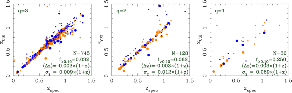
Figure 14.— CSI redshifts with $q=3,2,1$ plotted against redshifts in the VVDS and in the UDS from Cooper & Weiner (2013) with quality flags 3,4,5. Larger symbols indicate higher quality redshift flags from the high resolution datasets.

Table 2The Comparison of CSI Redshifts with Previously Published High Resolution Data

Range		$\sigma$	$N$	$N_{>0.10}$	$N_{>0.05}$
By Redshift
0.125	0.375	0.006	159	02	09
0.375	0.625	0.007	273	03	17
0.625	0.875	0.012	286	05	34
0.875	1.125	0.013	146	06	23
1.125	1.375	0.027	022	07	08
By $i$-band Magnitude
18.000	19.300	0.006	050	01	04
19.300	20.600	0.007	238	02	15
20.600	21.900	0.008	315	04	20
21.900	23.200	0.015	225	10	36
23.200	24.500	0.039	044	11	20
By $[3.6]$ Magnitude
18.000	18.600	0.006	061	00	06
18.600	19.200	0.007	202	02	15
19.200	19.800	0.009	200	06	17
19.800	20.400	0.010	215	11	31
20.400	21.000	0.012	207	13	32

In Figure 13 we show the $1\sigma$ scatters in magnitude bins, also derived using $\sigma=1.48\times$ MAD. Note that these values include a number of galaxies with low quality VVDS redshifts. For galaxies down to $i=23$ mag, the scatter is $\sigma_{z}/(1+z)=0.009$. Fainter than $i=23$ mag, the scatter rises to $\sigma_{z}/(1+z)=0.022$ (excluding those with $|\Delta z/(1+z)|>0.2$; $\sigma_{z}/(1+z)=0.029$ when these outliers are included). For galaxies with CSI redshifts between $0.9<z<1.2$, we find $\sigma_{z}/(1+z)=0.018$, though the distribution is non-Gaussian and the subsample contains a large fraction of objects with low quality VVDS redshifts. These standard deviations are reproduced in Table 2 along with the numbers of outliers with $|\delta z/(1+z)|>0.10$ and $>0.05$, and the total number of CSI measurements within each bin. Overall the median systematic bias in CSI redshifts is $\langle\delta z/(1+z)\rangle=-0.004$.

The consistency between our redshifts and those made available by the VVDS confirms that our procedures are working well. However, the number of high-resolution spectroscopic redshifts in the literature is too small to accurately characterize our redshift uncertainties in bins of magnitude, color, or spectral type using direct comparisons. Fortunately, we have two additional tests to help us probe the accuracy of our redshifts.

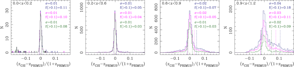
Figure 15.— A comparison of high quality CSI redshifts (with $q=3$) with those published by PRIMUS (Cool et al., 2013) in four redshift ranges. The comparison is shown using PRIMUS quality flags $2,3,4$ (blue), quality flags $3,4$ (violet), and quality flags $4$ (green). Overall agreement is excellent. Vertical lines show the 16th and 84th percentiles of the distribution, highlighting the tails of the distributions, and for the higher redshift bins, the dependence of the tails on PRIMUS quality flag. Above $z=0.6$ there is a pronounced tail of galaxies with CSI redshifts significantly higher than those measured by PRIMUS. This tail arises when galaxies with modestly strong [OII]3727Å emission (and blended with the 4000Å break) are fit with templates having a Balmer break and low (or no) levels of [OII]3727Å emission.

4.8.2 Direct Comparisons with Other Low-Resolution Redshifts

The SWIRE XMM-LSS field was also observed by the PRIMUS collaboration (Coil et al., 2011; Cool et al., 2013) who have published 213,696 redshifts, with 70,430 in fields that overlap with the CSI data presented here. In our “high-quality” CSI sample, 15,431 sources also have prism redshifts made available publicly by Cool et al. (2013). In Figure 15 we show histograms of the fractional redshift differences between CSI and PRIMUS for the 12,457 CSI measurements with $q=3$ in four increasing bins of redshift. Cool et al. (2013) published these redshifts with quality flags and we restrict the histograms to sets with PRIMUS flags $2,3,4$ (blue), $3,4$ (violet), and just $4$ (green).

In each panel we show standard deviations of the distributions as estimated from the MAD. We also show the fraction of CSI redshifts that differ from PRIMUS’s by more than 0.10 in $\delta z/(1+z)$. Overall, the level of agreement is very good given the strikingly different observing strategies, reduction techniques, and SED analysis. By itself this level of repeatability validates the approach of low dispersion spectroscopy. In the lowest redshift bin ($z<0.2$) there is a tail to low CSI redshifts. At such low redshifts the $u$-band can be an important redshift discriminant and some of this tail is due to our use of M-estimators that reduce the weight of “discrepant” data points in fitting templates to the SEDs. When an $r$-band point is discrepant, the effect is minimal due to the wavelength coverage of the spectra. But at $u$ there are no spectroscopic data to anchor the fit, and the net effect is to downweight the $u$ data (the issue is also relevant at $J$ and $K_{s}$). Future iterations of improvements to the SED fitting are expected to mitigate this (small) problem.

At $z>0.6$, as shown in the last two panels, the distributions have sharp cores peaked at zero but skew to positive redshift offsets compared to those from Cool et al. (2013). Based on our experience, and the experiences of Patel (2010), we suggest that this tail to higher CSI redshifts is the result of (1) differences between our templates, and (2) the broader wavelength baseline of the CSI SED fitting. Our theoretical templates have unrestricted emission line components in contrast to empirical templates. With empirically derived templates, the emission line measures are fixed by the set of galaxies (at lower redshift) that define the template set. In PRIMUS, the mean redshift defining the templates is $z\sim 0.3$ (Cool et al., 2013). Reproducing the potentially larger range of emission line luminosities (with respect to the underlying stellar continuum properties) at earlier epochs may be problematic.

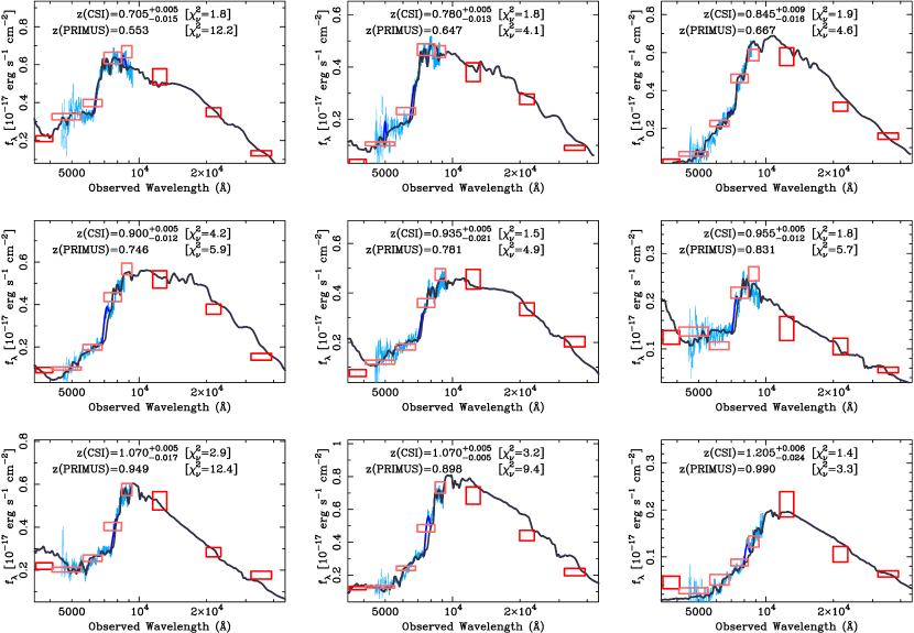
Figure 16.— Example galaxies from PRIMUS (Cool et al., 2013) where the CSI redshifts are higher, such that $0.05\Delta z/(1+z)<0.12$. Typically these galaxies have intermediate stellar populations, and the combination of [OII]3727Å line emission and the 4000Å and Balmer breaks all conspire with the low resolution to make fitting that region less robust. PRIMUS’s SED fitting did not include the wide wavelength baseline used by CSI, and thus could not provide the same leverage on those stellar population components that define the Balmer and 4000Å breaks. Furthermore, the PRIMUS redshifts were derived using empirical templates, which do not necessarily allow for the full range of emission line measures that may exist outside of the redshift range that defined the templates.

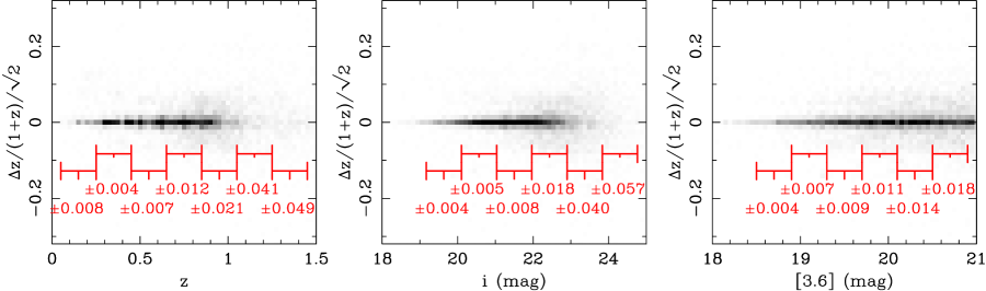
Figure 17.— Fractional redshift differences between repeat measurements, scaled by $\sqrt{2}$, as functions of redshift, $3.6\mu$m magnitude, and $i$-band magnitude for galaxies with $q\in\{2,3\}$. For example, at $0.6<z<0.8$, the half-width of the 68% confidence interval is $\sigma=0.009$. At $0.8<z<1.0$ we find $\sigma=0.020$. As seen in the comparison to VVDS, the width of the distribution is a stronger function of optical magnitude than near-IR magnitude, because our SED fitting is dominated by the IMACS spectroscopy. We find $\sigma=0.033$ at 22.6 mag $<i<$ 23.6 mag, and $\sigma=0.053$ at 23.6 mag $<i<$ 24.6 mag.

The allowed strength of [OII]3727Å line emission is important when the resolution is very low. Galaxies with weak (or no) [OII]3727Å line emission and a Balmer break indicative of intermediate age stars can sometimes be fit with templates that have [OII]3727Å line emission blended with the 4000Å break. This effect is similar to that seen in the low resolution spectroscopic study of A stars by Yu (1926), in which variable strengths of the lines in the Balmer series can shift the apparent location of the break. We show example SEDs in Figure 16 for galaxies at $z>0.6$ from the positive tail of the distribution of redshift differences between CSI and PRIMUS, listing both redshifts and the reduced $\chi^{2}$ we obtain for our best-fit templates at the CSI and PRIMUS redshifts. Note that many of these galaxies have modest [OII]3727Å and intermediate age stellar populations. The wide baseline of broadband photometry used by CSI helps constrain those stellar population components that define the 4000Å and Balmer breaks. We also take Figures 20 and 21 of Cool et al. (2013) as confirmation that these tails to high CSI redshifts are a reflection of these issues of resolution and feature strength. In those plots, Cool et al. (2013) shows that the PRIMUS redshift error distribution has a tail to negative redshift errors for galaxies at $z\lower 1.29167pt\hbox{$\scriptscriptstyle\;\buildrel>\over{\sim}\;$}0.6$. We take the dependence of this tail on PRIMUS’s quality flag (and the dependence of the tail in Figure 15 on the PRIMUS quality flag) as suggestive that the tail is due to PRIMUS’s systematic bias to low redshifts (for galaxies of this particular spectral type).

4.8.3 Uncertainties Derived from Repeat Measurements

Because the data from individual slit masks were reduced independently, repeat measurements can be compared. These comprise approximately 20% of the measured redshifts, providing a sample large enough to be analyzed as a function of galaxy properties, such as magnitude, color, stellar mass, or redshift. Without prior constraints or measurements for the derived properties of these objects we adopt the mean of multiple measurements when plotting or analyzing the distributions as functions of redshift. In Figure 17 we plot the 68% fractional redshift differences against redshift, as well as $3.6\mu$m and $i$-band magnitudes. As a function of redshift the half-width of the 68% interval is $0.009$ at $0.6<z<0.8$, $0.020$ for $0.8<z<1.0$, and $0.034$ for $1.0<z<1.2$. As can be seen in the third panel, the width of the distribution is a stronger function of optical magnitude than near-IR magnitude because our SED fitting is dominated by the IMACS spectroscopy. Currently, we find $\sigma=0.033$ at 22.6 mag $<i<$ 23.6 mag, and $\sigma=0.053$ at 23.6 mag $<i<$ 24.6 mag. Planned refinements in the pipeline are expected to improve the fidelity of the extracted spectra for such faint sources as our survey progresses.

The redshift uncertainties are dissected further in Figure 18 by breaking up the sample into three redshift ranges and plotting against $S/N$ ratios of the IMACS spectra, stellar mass, star formation activity, and rest frame $u-g$ color. From these panels it is evident that the redshift errors are not strongly correlated with spectral type or color, unlike the dependencies often seen in photometric redshifts. There is a rather small, subtle dependence on spectral type: quiescent galaxies (those with a negligible specific star formation rate and hence strong Balmer/4000Å breaks) and strongly star-forming galaxies have the greatest precision, while galaxies with modest or intermediate SFR have degraded redshift precision. Weak [OII]3727 Å emission at high redshift and observed at low resolution can appear blended with the 4000Å break and produce spectra that are reasonably well fit by an SED with a Balmer break and no [OII]3727 Å. More specifically, [OII]3727 Å is imperfectly correlated with the SFR inferred from the stellar continuum, leading to an additional uncertainty in the redshifts at the $\sim 0.01-0.02$ level in $\delta z/(1+z)$, depending on the $S/N$ ratio of the spectra, and even when not particularly statistically significant. This effect is substantially less pronounced for UDP data, where the higher resolution of the disperser shifts the wavelength of such [OII]3727Å confusion farther to the red. This power of the higher resolution UDP is illustrated in the last SED of Figure 9, in an old galaxy at $z=1.27$ with [OII]3727Å line emission (likely a LINER, e.g. Lemaux et al., 2010). Again, this problem with low resolution spectroscopy is only important for “green” galaxies; the bulk of the galaxy population, lying in the blue cloud and red sequence (with strong [OII]3727 Å and Balmer breaks respectively), is unaffected.

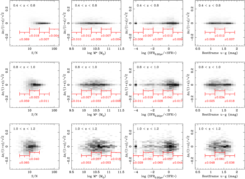
Figure 18.— Fractional redshift differences between repeat measurements, scaled by $\sqrt{2}$, as functions of $S/N$ ratio (75th percentile of the prism spectra), stellar mass, relative star formation activity, and restframe $u-g$ color for galaxies with $q\in\{2,3\}$. There is very little dependence of the redshift errors on spectral type or color, unlike what is typically seen for photometric redshifts.

While the abundance of repeat spectroscopic measurements has allowed us to characterize the redshift uncertainties, repeated spectra of any given object are fine-tuned with the same broadband photometry as described in Section 4.3. For some galaxies this can in principle introduce artificially tight correlations between the repeat spectroscopic measurements. Presumably, this issue becomes a serious problem only if the broad-band photometry is allowed to have greater weight in the likelihood analysis. This never occurs in our procedures because the number of data points in the UDP and LDP spectra far exceed the number of photometric bands. Even when the $S/N$ ratios of the spectra are low, binning these data over the photometric bandpasses yield $S/N$ ratios exceeding those of the broadband photometry for faint galaxies. However, since other factors (e.g., template selection) may produce artificially consistent repeat measurements, in the following section we employ one more independent test of the redshift uncertainties.

4.8.4 Uncertainties from Pairwise Velocity Distributions

Because galaxies largely exist in close pairs, in groups, in clusters, and in even larger coherent structures, all of which have velocity widths smaller than the redshift errors we expect in our data and analysis, the distribution of redshift errors can be inferred statistically from the distribution of pairwise redshift differences in a given sample. This technique was first explored and described by Quadri & Williams (2010) in an effort to derive the redshift uncertainties in photometric galaxy surveys, where a lack of spectroscopic follow-up and limited templates can hamper one’s ability to estimate uncertainties. Any methodology relying explicitly on clustering requires dense spatial sampling in order to extract a strong signal from the pairwise velocity histograms. While photometric redshift surveys, by definition, result in the highest possible spatial sampling, the spatial sampling of CSI is limited by slit collisions, limiting the number of galaxy pairs available to perform this analysis.

We divided our sample into subsets based on $i$-band magnitude and redshift and constructed pairwise velocity histograms. For the subsamples based on magnitude, we used those galaxies brighter than a given bin as a reference set, since those galaxies on average have more precise redshifts. While Quadri & Williams (2010) chose to randomize the positions in their dataset to correct for close pairs that arise only in projection, we opted to randomize the galaxy velocities since our slit-placement constraints lead to nontrivial spatial dependencies. Care was taken to properly normalize the histograms derived from the randomized distributions, as the number of galaxies in them, by definition, is too large by the number of galaxies within coherent velocity structures. Because this number cannot be precisely defined a priori, it must be deduced from the data — from the wings of the histograms. We made several realizations to reduce the Poisson noise imposed by the randomization process.

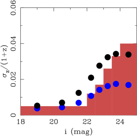
Figure 19.— A comparison of the redshift uncertainties derived from the pairwise velocity histogram method of Quadri & Williams (2010) with the mean uncertainty derived from the redshift likelihood functions. The red shaded bars trace the measured standard deviations from Gaussian fits to the pairwise velocity histograms as functions of magnitude. Using blue circles we plot the mean uncertainties derived from the 68% confidence limits for the individual galaxies. The black circles are derived assuming that the 95% confidence limits better represent the true redshift distribution, such that for multimodal likelihood functions these larger intervals better encompass any secondary (or tertiary) peaks. Overall, the comparison is quite good, suggesting that the uncertainties from our redshift fitting procedures are robust, with an increasing fraction of bimodal likelihood functions at faint magnitudes.

Figure 20.— (top) Distributions of high quality CSI redshifts ($q\in\{2,3\}$). (bottom) Distributions of high quality CSI redshifts for galaxies with stellar masses $1*<M/M*<2$ (orange) and $1/2<M/M_{*}<1$ (blue). A large portion of the apparent decline in $N(z)$ above $z=0.8$ is due to an increase in spectroscopic incompleteness (i.e. a declining success rate; see earlier discussion). The hatched regions mark the redshifts where these subsamples are affected by selection biases, such that the optical and IRAC limits exclude old stellar populations of a given stellar mass. For galaxies $M>M_{*}$, CSI is statistically correctable to $z\sim 1.45$. For galaxies $M>M_{*}/2$, CSI is correctable to $z=1.2$.

The pairwise velocity histograms were fit by Gaussians and the resulting standard deviations as a function of magnitude are plotted in Figure 19. Overplotted in blue are the expectations using the 68% confidence limits from our redshift likelihood functions, which are consistent with the pairwise velocity histograms down to $i\sim 23$ mag. We derived the black circles assuming that the 95% confidence limits better represent the true redshift error distribution. At faint optical magnitudes, the closer match of the black points with the red histogram reflects a shift from unimodal to bimodal redshift likelihood functions, where the 95% confidence limits probe both peaks while the 68% redshift confidence limits often do not fully encompass multiple peaks in bimodal (or trimodal) likelihood functions. The consistency demonstrated by the Quadri & Williams (2010) method, along with comparisons to other spectroscopic redshifts, has reinforced the validity of the redshift uncertainties derived from our generalized likelihood analysis down to faint magnitudes. For faint sources, even when bimodality of the likelihood functions becomes important, redshifts remain constrained on average to 0.05 or better in $\delta z/(1+z)$. This is consistent with the relative numbers of galaxies with redshift errors $>0.10$ and errors $>0.05$ in $\delta z/(1+z)$ seen in §4.8.1.

The striking agreement between the different methods of estimating redshift errors should be of general interest, since the Quadri & Williams (2010) method was in part devised to remedy the fact that photometric redshift surveys provide neither repeat measurements of a given galaxy nor high-resolution spectroscopy for most targets. Since any spatially dense survey will provide repeat measurements of (relatively) cold cosmic structures, the Quadri & Williams (2010) methodology remains a valuable technique for any spatially dense spectroscopic or photometric redshift survey — any survey where one does not have repeat observations with which to characterize uncertainties empirically.

Based on these three methods, we conclude that our random redshift uncertainties have been reliably characterized, and also that systematic uncertainties appear to be minimal. In particular we stress that our redshift errors are not strongly dependent on relative star formation activity, spectral type, or color. As discussed by Quadri et al. (2012), redshift errors that are strongly correlated with spectral type will bias estimates of local galaxy density if care is not taken to ensure that velocity windows (or line-of-sight linking lengths) encompass both red and blue galaxies with equal probability. Given CSI’s primary goal of characterizing galaxy properties as a function of environment, the relative insensitivity of our redshift errors on spectral type is a crucial point.

Figure 21.— (top) Applying completeness corrections, we convert the $N(z)$ of Figure 20 to the comoving number density of galaxies with stellar masses $1<M/M*<2$ (orange thick line) and $1/2<M/M_{*}<1$ (blue thick line). The redshift bins are defined by a constant comoving volume in which cosmic variance is $\sim 15\%$ for red galaxies (the hatched regions tracing the thick sold lines; Somerville et al., 2004). The large filled circles at $z=0.03$ are derived from GAMA (Baldry et al., 2012). The filled triangle at $z=1.5$ is derived from Marchesini et al. (2009). Open triangles are derived from the mass functions of Pozzetti et al. (2010). The open squares derive from the mass functions of Brammer et al. (2011). Open circles come from Ilbert et al. (2010). The galaxy number densities derived from PRIMUS (Moustakas et al., 2013) are represented by the smaller filled circles. The agreement with these past results is generally good with the exception of a large (2.5-$\sigma$) discrepancy between PRIMUS and CSI at $0.65<z<0.8$. The blue hashed region beyond $z=1.2$ shows approximately where the faint optical magnitude limit of the current analysis cuts the sample on the red sequence (see Figure 1) at $M=M_{*}/2$. (bottom) Using the same completeness corrections with the stellar mass estimates from the SED fitting, we compute the stellar mass density of the universe contained in galaxies within the given two mass bins. The points are the same as in (top), and the agreement between the stellar mass densities estimated here and past results is excellent.

5. Discussion

We conclude our discussion of the survey by presenting a broad overview of the CSI sample. Using the sample directly with the completeness functions derived earlier, we can estimate number densities of galaxies as a function of redshift and begin looking at galaxy quiescence and star formation activity. As we do so, the CSI selection limits are highlighted in order to give the reader a sense of the depth of the sample in luminosity, stellar mass, and redshift.

Figure 20 (top) shows the distribution of high quality CSI redshifts ($q\in\{2,3\}$) in the CFHTLS XMM field. The decrease in $N(z)$ above $z=0.8$ is due in part to the declining success rates and completeness at fainter optical magnitudes (as shown earlier). Figure 20 (bottom) dissects the sample into two stellar mass ranges, $1<M/M*<2$ (orange), and $1/2<M/M_{*}<1$ (blue). Our completeness functions derived earlier allow us to straightforwardly correct the observed numbers of galaxies in CSI to accurate number densities down to magnitude limits of $[3.6]=21$ mag and $i=24.5$ mag. At stellar masses of $M=M*$ and $M=M*/2$, we estimate that the magnitude limits impose selection biases at $z\lower 1.29167pt\hbox{$\scriptscriptstyle\;\buildrel>\over{\sim}\;$}1.45$ and $z\lower 1.29167pt\hbox{$\scriptscriptstyle\;\buildrel>\over{\sim}\;$}1.2$, respectively; these limits are shown as hatched regions with the respective color. Above these redshifts, the $i$-band and IRAC flux limits explicitly exclude galaxies from the selection and no statistically meaningful statements about the galaxy census can be made. However, below these redshifts these subsamples remain statistically correctable.

Knowing that our samples are relatively free from bias down to masses of $M>M*/2$ back to $z=1.2$, we apply completeness corrections and convert our $N(z)$ figures to estimates of the comoving number densities and stellar mass densities of galaxies as functions of redshift. The resulting CSI number densities are plotted using the thick lines in Figure 21. The number and mass densities are shown for two ranges of galaxy stellar mass, orange for $1<M/M*<2$, and dark blue for $1/2<M/M_{*}<1$. Within these redshift bins the estimated cosmic variance of $\sim 15\%$ dominates the uncertainties ($\sqrt{N}/N$ is small), and this uncertainty is shown by the hatched regions surrounding the thick orange and blue lines. The hatched regions shown at high redshift indicate redshifts where our faint magnitude limits impinge on these subsamples and the IRAC and $i$-band selections begin to exclude the oldest, passive galaxies. Down to the limits of CSI, Figure 21 reinforces what previous deep surveys covering smaller fields-of-view have found: a factor of two increase in the number densities of normal galaxies since $z=1$ (e.g., Drory et al., 2009; Marchesini et al., 2009; Ilbert et al., 2010; Moustakas et al., 2013).

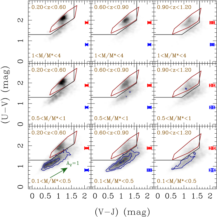
Figure 22.— Restframe $UVJ$ diagrams (e.g. Williams et al., 2009) for galaxies in CSI in several bins of redshift and stellar mass. The original Williams et al. (2009) $UVJ$ selection boundaries for quiescent galaxies are shown in black, superimposed on grayscale maps of the space density of galaxies at a given $U-V$ and $V-J$ color, mass, and redshift. The grayscales are fixed at a given mass scale to a range defined by our lowest redshift bin, to help illustrate the change in number density at high redshift at fixed mass. A green vector represents 1 mag of dust attenuation in the $V$-band for the Calzetti et al. (2000) extinction law. Blue contours highlight those galaxies with specific star formation rates $SSFR>2\times 10^{-10}$ yr^-1 (at $z=0.1$, evolving to $5.5\times 10^{-10}$ yr^-1 at $z=1$). These were derived using H$\alpha$ or [OII]3727Å, depending on the redshift, corrected for dust extinction using $A_{V}$ from the burst components of our SED fitting, and applying the conversion from Kennicutt (1998) or Kewley et al. (2004). The red polygon shows the locus of galaxies with $SSFR<10^{-11}$ yr^-1 (at $z=0.1$, evolving to $2.8\times 10^{-10}$ yr^-1 at $z=1$) with a range of metallicities from 1/10th to twice solar, and $0\leq A_{V}\leq 0.5$ mag of dust attenuation. We use these polygons to define a selection for quiescent galaxies in the following figures. Note that for galaxies with stellar masses $M<M*/2$ at $z\lower 1.29167pt\hbox{$\scriptscriptstyle\;\buildrel>\over{\sim}\;$}1.2$, the flux limits of CSI begin to select against quiescent galaxies, with these selection limits imposing on quiescent galaxies at lower masses at lower redshifts (see, e.g., Figure 2).

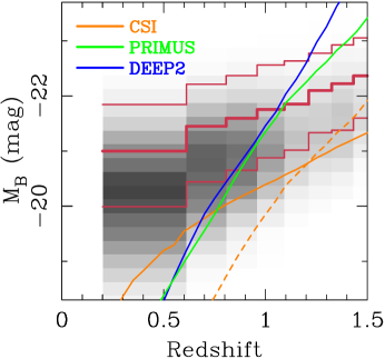
Figure 23.— The distribution of our $3.6\mu$m-selected galaxies in restframe $B$-band magnitude as a function of redshift. The green and blue lines indicate the approximate loci for old stellar populations at the limits of the PRIMUS and DEEP2 surveys. In orange, we show the CSI selection limit of $3.6\mu$m $=21$ mag (solid) and the effective optical limit of $i=24.5$ mag (dashed).

While a detailed analysis of this evolution is beyond the scope of this data paper, the power of CSI’s selection depth and field size is illustrated by dissecting the sample in some basic ways. Figure 22 presents CSI bicolor diagrams for several ranges of stellar mass and redshift. We have used our incompleteness functions and the $1/V_{max}$ method to compute the space densities of galaxies, represented using the grayscales. By fixing the grayscale ranges to that derived in the low redshift bin, one can directly see the evolution in number density at fixed mass that was shown in Figure 21.

These $UVJ$ diagrams are directly comparable to those by other authors (e.g. Williams et al., 2009; Whitaker et al., 2011), with the red clump of quiescent galaxies and the blue star forming sequence seen previously. The star forming sequence is especially prominent at low stellar masses. Using our H$\alpha$ and [OII]3727Å emission line luminosities to estimate rates of on-going star formation (e.g., Kennicutt, 1998; Kewley et al., 2004, after correcting for dust extinction), we identify those galaxies with high levels of star formation activity ($SSFR>2\times 10^{-10}$ yr^-1 at $z=0.1$, evolving to $5.5\times 10^{-10}$ yr^-1 at $z=1$) and show those with blue contours. These diagnostics reconfirm that the star-forming sequence in the $UVJ$ diagram remains an efficient means of selecting star-forming galaxies.

The red polygon shows the locus of galaxies with $-1\leq[Z/H]\leq 0.3$ and $A_{V}\leq 0.5$ and $SSFR<10^{-11}$ yr^-1 at $z=0.1$ ($2.8\times 10^{-10}$ yr^-1 at $z=1$). We can use this region to isolate galaxies with little, or no on-going star formation (such loci can be generated for such regions in any color space for any filter set). At late times there appears to be a tail out of the high-mass quiescent clump to blue colors along tracks such as those in Figure 4 of Patel et al. (2011) for old populations with very small recent star formation activity. But as Figure 21 already showed, there is a significant diminishing of galaxies with stellar masses $M>M*/2$ at high redshift, and because quiescent galaxies dominate at those mass scales, the red clump, in particular, is quite degraded by $z\sim 1$.

Being able to track this evolution as a function of mass requires significant depth and we highlight this point in Figure 23, showing the distribution of rest frame $B$-band absolute magnitude as a function of redshift. The irregular redshift bins used here are defined to have constant volume over the CSI sample, such that all bins have similar levels of cosmic variance ($\sim 15\%$; Somerville et al., 2004). The CSI $3.6\mu$m flux limit is shown by the solid orange lines, along with our effective optical limit of $i\approx 24.5$ mag as dashed orange lines. This $i$-band limit, where our spectroscopic completeness falls below 1/3 of the maximum (of 50% at $i=21$ mag, see Fig. 11), dominates over the IRAC selection at $z>1.2$. For comparison, we plot the DEEP2 and PRIMUS magnitude limits of $r=24.1$ mag and $i=23.0$ mag in Figure 23 using the blue and green lines, respectively. The red lines in Figure 23 show the 10th, 50th, and 90th percentiles of the stellar mass density residing in quiescent galaxies. By $z=1$, DEEP2 or PRIMUS are already missing half the stellar mass in quiescent galaxies.

Surveys like DEEP2 or PRIMUS probe unbiased samples only down to the present day stellar mass of the Milky Way at $z=0.9$, and half that at $z=0.75$. Although CSI’s additional reach to $z=1$ for these latter galaxies Way may only extend 1 Gyr farther back in cosmic time, the comoving volume covered within a constant area on the sky is nearly double that of PRIMUS. Such gains in sensitivity highlight the importance of an infrared selection in crafting an unbiased picture of galaxies since $z=1.5$. Furthermore, a methodology for measuring redshifts that does not depend crucially on the presence of emission lines at faint magnitudes, ensures that the resulting samples are relatively free from bias against galaxies with low $M/L$ ratios at fixed mass.

To better illustrate this point, Figure 24 shows a grayscale representation of the number densities of galaxies at a given stellar mass and redshift. The 10th, 50th, and 90th percentiles of the stellar mass density residing in quiescent galaxies are shown once again by the red lines. We model the selection differentially as a function of redshift, using the restframe colors of galaxies in each redshift slice to determine which ones get excluded by the survey flux limits at progressively higher redshifts (described in detail in a forthcoming CSI paper on the evolution of stellar mass and star formation), and derive linear fits to the evolution of these percentiles of the quiescent galaxy population. This evolution, or lack therefore, is shown using the dashed black lines in Figure 24 and is also visualized in the color-mass diagrams of Figure 25. The space densities of galaxies at a given restframe $u-g$ color and stellar mass are shown in three redshift bins in CSI, with orange hatched regions marking the projection of the CSI flux limits. The red contours trace the space densities of the quiescent galaxy population (see Figure 22). The 10th, 50th, and 90th percentiles in the stellar mass density for quiescent galaxies are overlaid using the vertical dashed lines, with the $0.2<z<0.4$ reference shown by the dotted lines. Our selection in the near-IR, and depth in the optical, ensures that CSI can trace at least 90% of the mass in quiescent galaxies back to early times. Each of these panels is normalized individually (unlike Figure 22), such that the grayscales and contour levels reflect consistent levels relative to the number densities at their respective epoch. The lack of any significant evolution in these percentiles (or in the red contours) indicates that those galaxies that become quiescent do so without preference for a particular mass scale (at least for galaxies above $M\gg 10^{10}M_{\odot}$), even as the number density of quiescent galaxies has more than doubled over the past 8.5 Gyr.

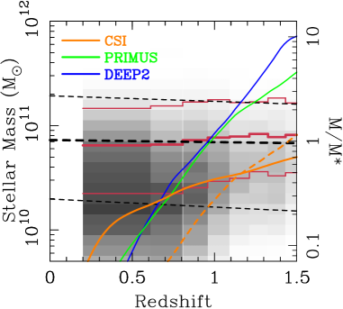
Figure 24.— The distribution of our $3.6\mu$m-selected galaxies in stellar mass, as functions of redshift The green and blue lines indicate the approximate loci for old stellar populations at the limits of the PRIMUS and DEEP2 surveys. In orange, we show the CSI selection limit of $3.6\mu$m $=21$ mag (solid) and the effective optical limit of $i=24.5$ mag (dashed). The red contours trace the 10th, 50th, and 90th percentiles of stellar mass density residing in quiescent galaxies. By carefully modeling the selection limits, we have computed corrections to these percentiles as functions of redshift and have estimated their linear evolution with redshift. The resulting, underlying evolution of the 10th, 50th, and 90th percentiles of the quiescent galaxy mass density are shown by the dashed black lines. Our selection in the near-IR, depth in the optical, observing strategy, reductions, and analysis of the data enable CSI to reach more than a magnitude fainter in the optical than DEEP2 or PRIMUS for passively evolving galaxies at $z=1$, enabling us to accurately trace the bulk of the stellar mass of passive and active galaxies to $z\sim 1.4$ in an unbiased fashion.

Figure 25.— Restframe color vs stellar mass for galaxies in three redshift bins in CSI, with the grayscale representing the number densities of galaxies at a given color and stellar mass. The 10th, 50th, and 90th percentiles in stellar mass density for quiescent galaxies at each epoch are shown by the vertical dashed lines. The vertical dotted lines show the equivalent percentiles derived from the $0.2<z<0.4$ subsample, highlighting the very low level of evolution in the overall shape of the quiescent galaxies mass function since $z\sim 1$. The orange hatched regions show the range of stellar mass and color where the CSI flux limits impinge on the sample. The red contours show (arbitrary) levels of galaxy number density for galaxies selected to be quiescent based on the $UVJ$ polygons of Figure 22. CSI is tracing the majority of stellar mass on the red sequence, with minimal bias against passive galaxies back almost 9 Gyr in cosmic time.

6. Summary

We have described the methodology behind, and initial data from, an ambitious new survey of approximately $2\times 10^{5}$ galaxies over a volume that encompasses the last 9 Gyr of cosmic history. By selecting a sample at 3.6$\mu$m from Spitzer-IRAC, the CSI survey is the most uniform to-date in terms of limiting mass as a function of redshift, and will ultimately cover an unbiased volume comparable to SDSS but at $0.5<z<1.5$. The power of the IMACS spectrograph with its low-resolution prisms allows us to survey large volumes efficiently and with sufficient spectral resolution to detect large-scale structure and to measure emission lines from strongly star-forming galaxies and AGN. CSI provides comparable redshift accuracies for red sequence and blue cloud galaxies; a significant advantage compared to many broadband photometric—and even some spectroscopic—studies. By combining our low-resolution spectrophotometry with extended broad-band photometry and sophisticated SED modeling, CSI bridges the gap between surveys that are deep enough to probe galaxies below M^∗ but are small in sample size and volume, and those large-sample, large-volume surveys that do not reach typical, Milky Way-like galaxies that are the main event in the history of cosmic evolution. In forthcoming papers we will update with more detail what we have learned from the first batch of CSI survey data.

One of the highest priority goals will be to take advantage of this large volume to simultaneously measure the evolution of the group mass function (e.g. Williams et al., 2012), and the dependence of star formation on environment (e.g. Kelson et al., 2014). In doing so CSI will uncover the extent to which the growth in the number density of passive galaxies over the past two-thirds of the lifetime of the universe can be attributed to group-related processes such as, for example, galaxy-galaxy interactions (leading to differential number density evolution between group and field galaxies), and/or a decrease in the available fuel for on-going star formation (leaving galaxy number densities unchanged). Given that most galaxies in virialized or massive groups (or both) are “red and dead” even at $z\sim 1$ (Kelson et al., 2014), the mass selection, high spectral coverage, and color-insensitive redshift accuracy of CSI will all be critical elements in characterizing relatively poor groups at high redshift. Subsequent CSI analyses will also focus on, for example, AGN and any connections to group and/or host galaxy properties, on differences between centrals and satellites (e.g. Berlind & Weinberg, 2002; Weinmann et al., 2006; van den Bosch et al., 2007), and on merger rates (e.g. Williams et al., 2011) as functions of environment.

7. acknowledgments

D.D.K. expresses his appreciation to his co-investigators for their patience. The whole team also appreciates the enormous contributions of the Carnegie Institution for Science to the project, from the new disperser in IMACS, to the computing cluster in the basement, to the generosity of the Time Assignment Committee. Furthermore, the comments from the anonymous referee are acknowledged; they were enormously helpful, in particular, in prompting us to improve the discussions of incompleteness, and inspiring us to rethink how to quantify data quality. We are grateful to NOAO for its contributions and to the astronomical community for its awarding of survey status to CSI in 2009. R.J.W. also gratefully acknowledges support from NSF Grant AST-0707417. Based, in part, on observations obtained with MegaPrime/MegaCam, a joint project of CFHT and CEA/DAPNIA, at the Canada-France-Hawaii Telescope (CFHT) which is operated by the National Research Council (NRC) of Canada, the Institut National des Science de l’Univers of the Centre National de la Recherche Scientifique (CNRS) of France, and the University of Hawaii. This work is based in part on data products produced at TERAPIX and the Canadian Astronomy Data Centre as part of the Canada-France-Hawaii Telescope Legacy Survey, a collaborative project of NRC and CNRS. This publication makes use of data products from the Two Micron All Sky Survey, which is a joint project of the University of Massachusetts and the Infrared Processing and Analysis Center/California Institute of Technology, funded by the National Aeronautics and Space Administration and the National Science Foundation

References

- Abraham et al. (2004) Abraham, R. G., et al. 2004, AJ, 127, 2455
- Aird et al. (2012) Aird, J., Coil, A. L., Moustakas, J., et al. 2012, ApJ, 746, 90
- Aird et al. (2013) Aird, J., Coil, A. L., Moustakas, J., et al. 2013, arXiv:1301.1689
- Akiyama et al. (2010) Akiyama, M., 2010, in preparation
- Autry et al. (2003) Autry, R. G., Probst, R. G., Starr, B. M., et al. 2003, Proc. SPIE, 4841, 525
- Baldry et al. (2012) Baldry, I. K., Driver, S. P., Loveday, J., et al. 2012, MNRAS, 421, 621
- Beers et al. (1990) Beers, T. C., Flynn, K., & Gebhardt, K. 1990, AJ, 100, 32
- Bell & de Jong (2001) Bell, E. F., & de Jong, R. S. 2001, ApJ, 550, 212
- Berlind & Weinberg (2002) Berlind, A. A., & Weinberg, D. H. 2002, ApJ, 575, 587
- Bertin & Arnouts (1996) Bertin, E., & Arnouts, S. 1996, A&AS, 117, 393
- Brammer et al. (2011) Brammer, G. B., Whitaker, K. E., van Dokkum, P. G., et al. 2011, ApJ, 739, 24
- Bruzual & Charlot (2003) Bruzual, G., & Charlot, S. 2003, MNRAS, 344, 1000
- Calzetti et al. (2000) Calzetti, D., Armus, L., Bohlin, R. C., et al. 2000, ApJ, 533, 682
- Carlberg et al. (2001) Carlberg, R. G., Yee, H. K. C., Morris, S. L., et al. 2001, ApJ, 552, 427
- Carlberg et al. (1997) Carlberg, R. G., Yee, H. K. C., Ellingson, E., et al. 1997, ApJ, 485, L13
- Coil et al. (2011) Coil, A. L., Blanton, M. R., Burles, S. M., et al. 2011, ApJ, 741, 8
- Cool et al. (2013) Cool, R. J., Moustakas, J., Blanton, M. R., et al. 2013, ApJ, 767, 118
- Cooper & Weiner (2013) Cooper, M. C., & Weiner B., in preparation
- Cuillandre & Bertin (2006) Cuillandre, J.-C., & Bertin, E. 2006, SF2A-2006: Semaine de l’Astrophysique Francaise, 265
- Dierckx (1993) Dierckx, P., Curve and Surface Fitting with Splines, New York: Oxford University Press, 1993
- Dressler et al. (2011) Dressler, A., Bigelow, B., Hare, T., et al. 2011, PASP, 123, 288
- Drory et al. (2009) Drory, N., Bundy, K., Leauthaud, A., et al. 2009, ApJ, 707, 1595
- Glazebrook & Bland-Hawthorn (2001) Glazebrook, K., & Bland-Hawthorn, J. 2001, PASP, 113, 197
- Halliday et al. (2008) Halliday, C., Daddi, E., Cimatti, A., et al. 2008, A&A, 479, 417
- Högbom (1974) Högbom, J. A. 1974, A&AS, 15, 417
- Horne (1986) Horne, K. 1986, PASP, 98, 609
- Huber (1981) Huber, P. J. Robust Statistics. John Wiley & Sons, New York, 1981
- Ilbert et al. (2010) Ilbert, O., Salvato, M., Le Floc’h, E., et al. 2010, ApJ, 709, 644
- Kauffmann et al. (2004) Kauffmann, G., White, S. D. M., Heckman, T. M., Ménard, B., Brinchmann, J., Charlot, S., Tremonti, C., & Brinkmann, J. 2004, MNRAS, 353, 713
- Kelson et al. (2014) Kelson, D. D., et al. 2014, ApJ, in prep
- Kennicutt (1998) Kennicutt, R. C., Jr. 1998, ARA&A, 36, 189
- Kewley et al. (2004) Kewley, L. J., Geller, M. J., & Jansen, R. A. 2004, AJ, 127, 2002
- Kroupa (2001) Kroupa, P. 2001, MNRAS, 322, 231
- Le Fevre et al. (2003) Le Fevre, O., Vettolani, G., Maccagni, D., et al. 2003, Proc. SPIE, 4834, 173
- Lemaux et al. (2010) Lemaux, B. C., Lubin, L. M., Shapley, A., et al. 2010, ApJ, 716, 970
- Lonsdale et al. (2003) Lonsdale, C. J., et al. 2003, PASP, 115, 897
- Maraston (2005) Maraston, C. 2005, MNRAS, 362, 799
- Marchesini et al. (2009) Marchesini, D., van Dokkum, P. G., Förster Schreiber, N. M., et al. 2009, ApJ, 701, 1765
- McMillan (2011) McMillan, P. J. 2011, MNRAS, 414, 2446
- Mendez et al. (2013) Mendez, A. J., Coil, A. L., Aird, J., et al. 2013, ApJ, 770, 40
- Moustakas et al. (2013) Moustakas, J., Coil, A. L., Aird, J., et al. 2013, ApJ, 767, 50
- Patel et al. (2009a) Patel, S. G., Kelson, D. D., Holden, B. P., Illingworth, G. D., Franx, M., van der Wel, A., & Ford, H. 2009, ApJ, 694, 1349
- Patel et al. (2009b) Patel, S. G., Holden, B. P., Kelson, D. D., Illingworth, G. D., & Franx, M. 2009, ApJ, 705, L67
- Patel (2010) Patel, S. 2010, Ph.D. Thesis, University of California, Santa Cruz
- Patel et al. (2011) Patel, S. et al. 2011, ApJ, 735, 53
- Patel et al. (2012) Patel, S. G., Holden, B. P., Kelson, D. D., et al. 2012, ApJ, 748, L27
- Pozzetti et al. (2010) Pozzetti, L., Bolzonella, M., Zucca, E., et al. 2010, A&A, 523, A13
- Quadri & Williams (2010) Quadri, R. F., & Williams, R. J., (2010), ApJ, 725, 794
- Quadri et al. (2012) Quadri, R. F., Williams, R. J., Franx, M., & Hildebrandt, H. 2012, ApJ, 744, 88
- Simpson et al. (2010) Simpson, C., 2010, in preparation
- Skrutskie et al. (2006) Skrutskie, M. F., et al. 2006, AJ, 131, 1163
- Smail et al. (2008) Smail, I., Sharp, R., Swinbank, A. M., et al. 2008, MNRAS, 389, 407
- Sorba & Sawicki (2010) Sorba, R., & Sawicki, M. 2010, ApJ, 721, 1056
- Somerville et al. (2004) Somerville, R.S, et al. 2004, ApJ, 600, L171
- Surace et al. (2005) Surace, J. et al. 2005, preprint
- Tinsley (1972) Tinsley, B. M. 1972, ApJ, 178, 319
- van den Bosch et al. (2007) van den Bosch, F. C., Yang, X., Mo, H. J., et al. 2007, MNRAS, 376, 841
- Weinmann et al. (2006) Weinmann, S. M., van den Bosch, F. C., Yang, X., & Mo, H. J. 2006, MNRAS, 366, 2
- Whitaker et al. (2011) Whitaker, K. E., Labbé, I., van Dokkum, P. G., et al. 2011, ApJ, 735, 86
- Williams et al. (2009) Williams, R. J., Quadri, R. F., Franx, M., van Dokkum, P., & Labbé, I. 2009, ApJ, 691, 1879
- Williams et al. (2011) Williams, R. J., Quadri, R. F., & Franx, M. 2011, ApJ, 738, L25
- Williams et al. (2012) Williams, R. J., et al. 2012, ApJ, 749, L12
- Willmer et al. (2006) Willmer, C. N. A., et al. 2006, ApJ, 647, 853
- Wright et al. (1994) Wright, E. L., Eisenhardt, P. E., & Fazio, G. G. 1994, arXiv:astro-ph/9407055
- Yu (1926) Yu, C.-S. 1926, Lick Observatory Bulletin, 12, 104
- Zhang (1997) Zhang, Z. 1997, Image and Vision Computing, 15, 59