The fixation time of a strongly beneficial allele in a structured population

Abstract

For a beneficial allele which enters a large unstructured population and eventually goes to fixation, it is known that the time to fixation is approximately $2\log(\alpha)/\alpha$ for a large selection coefficient $\alpha$. For a population that is distributed over finitely many colonies, with migration between these colonies, we detect various regimes of the migration rate $\mu$ for which the fixation times have different asymptotics as $\alpha\to\infty$.

If $\mu$ is of order $\alpha$, the allele fixes (as in the spatially unstructured case) in time $\sim 2\log(\alpha)/\alpha$. If $\mu$ is of order $\alpha^{\gamma},0\leq\gamma\leq 1$, the fixation time is $\sim(2+(1-\gamma)\Delta)\log(\alpha)/\alpha$, where $\Delta$ is the number of migration steps that are needed to reach all other colonies starting from the colony where the beneficial allele appeared. If $\mu=1/\log(\alpha)$, the fixation time is $\sim(2+S)\log(\alpha)/\alpha$, where $S$ is a random time in a simple epidemic model.

The main idea for our analysis is to combine a new moment dual for the process conditioned to fixation with the time reversal in equilibrium of a spatial version of Neuhauser and Krone’s ancestral selection graph.

all math.PR/1402.1769

, ,
  and

1 Introduction

The goal of this paper is the asymptotic analysis of the time which it takes for a single strongly beneficial mutant to eventually go to fixation in a spatially structured population. The beneficial allele and the wildtype will be denoted by $\mathpzc B$ and $\mathpzc b$, respectively. The evolution of type frequencies is modelled by a $[0,1]^{d}$-valued diffusion process $\mathcal{X}=(\underline{X}(t))_{t\geq 0},\underline{X}(t)=(X_{i}(t))_{i=1,\dots,d}$, where $d\in\{2,3,\ldots\}$ denotes the number of colonies and $X_{i}(t)$ stands for the frequency of the beneficial allele $\mathpzc B$ in colony $i$ at time $t$. The dynamics accounts for resampling, selection and migration. The process $\mathcal{X}$ is started at time $0$ by an entrance law from $\underline{0}:=(0,\ldots,0)$ and is conditioned to eventually hit $\underline{1}:=(1,\ldots,1)$.

Models of this kind are building blocks for more complex ones that are used to obtain predictions for genetic diversity patterns under various forms of selection. Indeed, together with the strongly beneficial allele, neutral alleles at physically linked genetic loci also have the tendency to go to fixation, provided these loci are not too far from the selective locus under consideration. This so-called genetic hitchhiking was first modelled by Maynard Smith and Haigh (1974). A synonymous notion is that of a selective sweep, which alludes to the fact that, after fixation of the beneficial allele $\mathpzc B$, neutral variation has been swept from the population. Important tools were developed from these patterns to locate targets of selection in a genome and quantify the role of selection in evolution, see e.g. reviews in Sabeti et al. (2006), Nielsen (2005), Thornton et al. (2007).

The process of fixation of a strongly beneficial mutant in the panmictic (i.e. unstructured) case has been studied using a combination of techniques from diffusion processes and coalescent processes in a random background; see e.g. Kaplan et al. (1989), Stephan et al. (1992), Schweinsberg and Durrett (2005), Etheridge et al. (2006). However, since the analytical tools applied in these papers rely on the theory of one-dimensional diffusion processes, the extension of these results to a spatially structured situation is far from straight-forward.

The starting point for the tools developed in this paper is the ancestral selection graph (ASG) of Neuhauser and Krone (1997). This process has been introduced in order to study the genealogy under models including selection. Although the ASG can in principle be used for an arbitrary strength of selection, it has been employed mainly for models of weak selection, since then the resulting genealogy is close to a neutral one. However, Wakeley and Sargsyan (2009) have used the ASG for strong balancing selection and Pfaffelhuber and Pokalyuk (2013) have shown how to use the ASG in order to re-derive classical results for selective sweeps in a panmictic population. In our present work a spatial version of the ASG is the tool of choice which carries over from the panmictic to the structured case, thus extending the techniques developed in Pfaffelhuber and Pokalyuk (2013) and leading to new results for the spatially structured case. The key idea here is to employ the equilibrium ASG in a “paintbox representation” of the (fixed time) distributions of the type frequency process conditioned to eventual fixation, and then use time reversal of the equilibrium ASG to obtain an object accessible to the asymptotic analysis.

The fixation process in a structured population under selection has been the object of study before. Slatkin (1981) and Whitlock (2003) give heuristic results and comparisons to the panmictic case. While the former paper only gives results for strong selection but very weak migration, the latter study gives a comparison to the panmictic case and studies the question which parameters should be used in the panmictic setting in order to approximate fixation probabilities and fixation times for structured populations. In Kim and Maruki (2011) the above studies are extended by analysing in addition the expected heterozygosity of linked neutral loci in the case of frequent migration for populations structured according to a circular stepping-stone model, see also Remark 2.7 below. Hartfield (2012) gives a more thorough analysis of the fixation times for large selection/migration ratios in general stepping-stone populations based on the assumption that in each colony the beneficial mutation spreads before migrating.

Our investigation will provide rigorous results on fixation times for structured populations, and will detect the corresponding regimes of relative migration/selection speed.

Outline of the paper.

After introducing the model in Section 2 we formulate our main results. These concern the existence of solutions and the structure of the set of solutions of the system of SDEs specified in our model (Theorem 1) and the asymptotics of the fixation times for a strongly beneficial allele $\mathpzc B$ in a structured population (Theorem 2). For the panmictic case (i.e. $d=1$), it is well-known that the fixation time, for a large selection coefficient $\alpha$, is approximately $2\log(\alpha)/\alpha$. As it turns out, the time-scale of $\log(\alpha)/\alpha$ applies in our spatial setting as well. However, population structure may slow down the fixation process. We study this deceleration for various regimes of the migration rate $\mu$. A spatial version of the ancestral selection graph is introduced in Section 3, and its role in the analysis of the fixation probability and the fixation time by the method of duality is clarified. This leads to a proof of Theorem 1 in Sec. 3.9, and to the key Proposition 3.1 which relates the asymptotic distribution of the fixation time of the Wright-Fisher system to that of a marked particle system. Based on the latter, the proof of Theorem 2 is completed in Sec. 4.

2 Model and main results

We consider solutions $\mathcal{X}=(\underline{X}(t))_{t\geq 0}$, $\underline{X}(t)=(X_{1}(t),\dots,X_{d}(t))\in[0,1]^{d}$, of the system of interacting Wright-Fisher diffusions

$$dX_{i} =\Big{(}\alpha X_{i}(1-X_{i})+\mu\sum_{j=1}^{d}b(i,j)(X_{j}-X_{i})\Big{)}dt+\sqrt{\frac{1}{\rho_{i}}X_{i}(1-X_{i})}dW_{i},$$

$$\qquad\qquad\qquad\qquad\qquad\qquad\qquad\qquad\qquad\qquad\qquad\qquad i=1,\dots,d$$ (2.1)

for independent Brownian motions $W_{1},\dots,W_{d}$. Here, $\alpha$ and $\mu$ are positive constants (the selection and migration coefficient), and $b(i,j)$, $i,j=1,\ldots,d$, $i\neq j$, are non-negative numbers (the backward migration rates) that constitute an irreducible rate matrix $\underline{\underline{b}}$ whose unique equilibrium distribution has the weights $\rho_{1},\dots,\rho_{d}$ (which stand for the relative population sizes of the colonies). It is well-known (see e.g. Dawson (1993)) that the system (2) has a unique weak solution.

Equation (2) models the evolution of the relative frequencies of the beneficial allele at the various colonies, assuming a migration equilibrium between the colonies. The “gene flow” from colony $i$ to colony $j$ is $\rho_{i}\mu a(i,j)=\rho_{j}\mu b(j,i)$; here, $\underline{\underline{a}}=(a(i,j))$ with

$$a(i,j)=\frac{\rho_{j}}{\rho_{i}}b(j,i)$$ (2.2)

is the matrix of forward migration rates.

Remark 2.1 (Limit of Moran models).

We note in passing that the process $\mathcal{X}$ arises as the weak limit (as $N\to\infty$) of a sequence of structured two-type Moran models with $N$ individuals. The dynamics of this Moran model is local pairwise resampling with rates $1/\rho_{i}$, selection with coefficient $\alpha$ (i.e. offspring from every beneficial line in colony $i$ replaces some line in the same colony at rate $\alpha$; note that this is the same as selection events which occur at rate $s:=\frac{\alpha}{N}$ for each (ordered) pair of particles) and migration with rates $\mu a(i,j)$ per line. Considering now the relative frequencies of the beneficial type at the various colonies and letting $N\to\infty$ gives (2). Here, our assumption that $(\rho_{i})$ constitutes an equilibrium for the migration ensures that we are in a demographic equilibrium with asymptotic colony sizes $\rho_{i}N$ (otherwise the $\rho_{i},\,\rho_{j}$ in the formulas would have to be replaced by time-dependent intensities).

We define the fixation time of $\mathcal{X}$ as

$$T_{\text{fix}}:=\inf\{t>0:\underline{X}(t)=\underline{1}\}.$$ (2.3)

The fixation probability of the system (2), started in $\underline{X}(0)=\underline{x}$, is well-known (see Nagylaki (1982)). In Corollary 3.9 we will provide a new proof for the formula

$$\mathbf{P}_{\underline{x}}(T_{\text{fix}}<\infty)=\frac{1-e^{-2\alpha(x_{1}\rho_{1}+\cdots+x_{d}\rho_{d})}}{1-e^{-2\alpha}}.$$ (2.4)

Since fixation of the beneficial allele, $\{T_{\text{fix}}<\infty\}$, is an event in the terminal $\sigma$-algebra of $\mathcal{X}$, conditioning on this event leads to an $h$-transform of (2) which turns out to be given by the system of SDEs

$$dX^{\ast}_{i} =\Big{(}\alpha X^{\ast}_{i}(1-X^{\ast}_{i})\coth\Big{(}\alpha\sum_{j=1}^{d}X^{\ast}_{j}\rho_{j}\Big{)}+\mu\sum_{j=1}^{d}b(i,j)(X^{\ast}_{j}-X^{\ast}_{i})\Big{)}dt$$

$$\qquad\qquad\qquad\qquad\qquad\qquad\qquad\qquad\qquad\quad+\sqrt{\frac{1}{\rho_{i}}X^{\ast}_{i}(1-X^{\ast}_{i})}dW_{i}$$ (2.5)

for $i=1,\dots,d$, with $\coth(x)=\frac{e^{2x}+1}{e^{2x}-1}$. The uniqueness of the solution of  (2) carries over to that of (2) as long as $\underline{x}\neq\underline{0}$. For $\underline{x}=\underline{0}$, the right hand side of (2) is not defined, and we have to talk about entrance laws from $\underline{0}$ for solutions of (2) in this case.

Definition 2.2 (Entrance law from $\underline{0}$).

Let $((\underline{X}^{\ast}(t))_{t>0},\mathbf{P})$ with $\underline{X}^{\ast}(t)=(X^{\ast}_{1}(t),...,X^{\ast}_{d}(t))$ be a solution of (2) such that $\underline{X}^{\ast}(t)\neq\underline{0}$ for $t>0$ and $\underline{X}^{\ast}(t)\xrightarrow{t\to 0}\underline{0}$ in probability. Then, the law of $\underline{X}^{\ast}$ under $\mathbf{P}$ is called an entrance law from $\underline{0}$ for the dynamics (2).

The following is shown in Section 3.9.

Theorem 1.

a) For $\underline{x}\in[0,1]^{d}\setminus\{\underline{0}\}$, the system (2) has a unique weak solution.
b) Every entrance law from $\underline{0}$ is a convex combination of $d$ extremal entrance laws from $\underline{0}$, which we denote by $\mathbf{P}^{i}_{\underline{0}}(\mathcal{X}^{\ast}\in(.))$, with $(\mathcal{X}^{\ast},\mathbf{P}^{i}_{\underline{0}})$ arising as the limit in distribution of $(\mathcal{X}^{\ast},\mathbf{P}_{\varepsilon\underline{e}_{i}})$ as $\varepsilon\to 0$, where $\underline{e}_{i}$ is the vector whose $i$-th component is 1 and whose other components are $0$.

Remark 2.3 (Interpretation of the extremal solutions).

We call $(\mathcal{X}^{\ast},\mathbf{P}^{\iota}_{\underline{0}})$ the solution with the founder in colony $\iota$. In intuitive terms the case $\underline{x}=\underline{0}$ corresponds to the beneficial allele $\mathpzc B$ being present in a copy number which is too low to be seen in a very large population, i.e. on a macroscopic level. In this case, since the process is conditioned on fixation, there is exactly one individual – called founder – which will be the ancestor of all individuals at the time of fixation. This intuition is made precise in a picture involving duality, see Section 3.7. The $d$ different entrance laws from $\underline{0}$ belonging to (2) correspond to the $d$ different possible geographic locations of the founder.

Before stating our main result on the fixation time of the system (2) we fix some notation and formulate one more definition.

Remark 2.4 (Notation).

To facilitate notation we will use Landau symbols. For functions $f,g:\mathbb{R}\to\mathbb{R}$, we write (i) $f=\mathcal{O}(g)$ as $x\to x_{0}\in\overline{\mathbb{R}}$ if $\limsup_{x\to x_{0}}|f(x)/g(x)|<\infty$, (ii) $f\in\Theta(g)$ if and only if $f\in\mathcal{O}(g)$ and $g\in\mathcal{O}(f)$ and (iii) $f\sim g$ as $x\to x_{0}$ if and only if $f(x)/g(x)\xrightarrow{x\to x_{0}}1$, (iv) $f=o(g)$ as $x\to x_{0}\in\overline{\mathbb{R}}$ if $\limsup_{x\to x_{0}}|f(x)/g(x)|=0$. We write $\xRightarrow{}$ for convergence in distribution and $\xrightarrow{}_{p}$ for convergence in probability.

In the case of a single colony ($d=1$) we have $T_{\rm{fix}}\sim 2\log\alpha/\alpha$ as $\alpha\to\infty$. Indeed, it is well known that in this case the conditioned diffusion (2) can be separated into three phases (Etheridge et al., 2006): the beneficial allele $\mathpzc B$ first has to increase up to a (fixed) small $\varepsilon>0$. This phase lasts a time $\sim\log(\alpha)/\alpha$. In the second phase, the frequency increases to $1-\varepsilon$ in time of order $1/\alpha$ which is short as compared to the first and third phase. In the third phase, it takes still about time $\log(\alpha)/\alpha$ until the allele finally fixes in the population.

Definition 2.5 (Two auxiliary epidemic processes).

Let $\underline{\underline{a}}$ be the matrix of forward migration rates and let $G=(V,E)$ be the (connected) graph with vertex set $1,\dots,d$ and edge set $E:=\{(i,j):a(i,j)>0\}.$ We need two auxiliary processes in order to formulate our theorem.

1. For $\gamma\in[0,1]$ and $\iota\in\{1,\dots,d\}$, consider the (deterministic) process $\mathcal{I}^{\iota,\gamma}:=\mathcal{I}^{\iota}=(\underline{I}^{\iota}(t))_{t\geq 0}$, $\underline{I}^{\iota}(t)=(I_{1}^{\iota}(t),\dots,I_{d}^{\iota}(t))$, with state space $\{0,1\}^{d}$ defined as follows: The process starts in $I^{\iota}_{j}(0)=\delta_{\iota j},j=1,...,d$. As soon as one component ($I_{k}^{\iota}$, say) reaches $1$, then after the additional time $1-\gamma$ all those components $I^{\iota}_{j}$ for which $a(k,j)>0$ are set to 1. The fixation time of this process will be denoted by

   $$S_{\mathcal{I}^{\iota,\gamma}}:=\inf\{t\geq 0:\underline{I}^{\iota}(t)=\underline{1}\}.$$

   In other words, $S_{\mathcal{I}^{\iota,\gamma}}=(1-\gamma)\Delta_{\iota}$, where $\Delta_{\iota}$ is the number of steps that are needed to reach all other vertices of the graph $G$ in a stepwise percolation starting from $\iota$. An intuitive interpretation is as follows: State 1 of a component means that the colony is infected (by the beneficial type $\mathpzc B$) and state $0$ means that it is not infected. If a colony gets infected (at time $t$, say), then all the neighbouring (not yet infected) colonies get infected precisely at time $t+1-\gamma$.

2. For any $\iota\in\{1,\dots,d\}$, consider the (random) process $\mathcal{J}^{\iota}=(\underline{J}^{\iota}(t))_{t\geq 0}$, $\underline{J}^{\iota}(t)=(J_{1}^{\iota}(t),\dots,J_{d}^{\iota}(t))$, with state space $\{0,1,2\}^{d}$. In state 0, the colony is not infected, in state 1 it is infected but still not infectious, and in 2, it is infectious. The initial state is $J^{\iota}_{\iota}(0)=1$ and $J^{\iota}_{j}(0)=0$ for $j\neq\iota$, where $\iota$ is the founder colony. Transitions from state 1 to state 2 occur exactly one unit of time after entering state 1. For $j\neq\iota$, transitions from 0 to 1 occur at rate $2\sum_{k}\rho_{k}a(k,j)\mathbf{1}_{\{J^{\iota}_{k}=2\}}$. The fixation time of this process will be denoted by

   $$S_{\mathcal{J}^{\iota}}:=\inf\{t\geq 0:\underline{J}^{\iota}(t)=\underline{2}\};$$

   in particular, this time is larger than $1$.

Infection in these epidemic processes indicates presence of the beneficial type. Our second main result quantifies in terms of these processes how various migration rates affect the spread and the fixation time of the beneficial type.

Theorem 2 (Fixation times of $\mathcal{X}^{\ast}$).

For $\iota\in\{1,\ldots,,d\}$, let $\mathcal{X}^{\ast}=(\underline{X}^{\ast}(t))_{t\geq 0}$ be the solution of (2) with $\underline{X}^{\ast}(0)=\underline{0}$ and with the founder in colony $\iota$, see Remark 2.3. Then, depending on the scaling ratio between $\mu$ and $\alpha$ as $\alpha\to\infty$, we have the following asymptotics for the fixation time $T_{\rm fix}$ defined in (2.3) (now for $\underline{\mathcal{X}}^{\ast}$ in place of $\underline{\mathcal{X}}$):

1. If $\mu\in\Theta(\alpha)$, then

   $$\frac{\alpha}{\log\alpha}T_{\rm{fix}}\xrightarrow{\alpha\to\infty}_{p}2.$$

2. More generally, if $\mu\in\Theta(\alpha^{\gamma})$ for some $\gamma\in[0,1]$, then

   $$\frac{\alpha}{\log\alpha}T_{\rm{fix}}\xrightarrow{\alpha\to\infty}_{p}S_{\mathcal{I}^{\iota,\gamma}}+2.$$

3. If $\mu=\frac{1}{\log\alpha}$, then

   $$\frac{\alpha}{\log\alpha}T_{\rm{fix}}\xRightarrow{\alpha\to\infty}S_{\mathcal{J}^{\iota}}+1.$$

Remark 2.6.

[Interpretation] Let us briefly give some heuristics for the three cases of the Theorem. The bottomline of our argument is this: Given a colony $i$ is already “infected” by the beneficial mutant, the most probable scenario (as $\alpha\to\infty$) is that the beneficial type in colony $i$ grows until migration exports the beneficial type to other colonies which can be reached from colony $i$. We argue with successful lines, which are – in a population undergoing Moran dynamics as in Remark 2.1 – individuals whose offspring are still present at the time of fixation.

For notational simplicity, we discuss here the situation $d=2$ with the founder of the sweep being in colony $\iota=1$. The three cases allow us to distinguish when the first successful migrant (carrying allele $\mathpzc B$ and still having offspring at the time of fixation) moves to colony 2.

(A) $\mu\in\Theta(\alpha^{\gamma})$

(B) $\mu=1/(\log(\alpha))$

Figure 1: Two examples of a sweep in a structured population of $d=2$ colonies. (A) For $\mu\in\Theta(\alpha^{\gamma})$, the epidemic model $\mathcal{I}^{1,\gamma}$ from Theorem 2 starts with ${\underline{I}}^{1}(0)=(1,0)$. The first successful migrant transports the beneficial allele to colony 2 at time $1-\gamma$ (on the time-scale $\log(\alpha)/\alpha$). Hence, fixation occurs approximately at time $(3-\gamma)\log(\alpha)/\alpha$. (B) For $\mu=1/(\log\alpha)$, the epidemic model ${\mathcal{J}}^{1}$ from Theorem 2 starts with ${\underline{J}}^{1}(0)=(1,0)$. The first successful migrant transports the beneficial allele to colony 2 at time $1+X$, where $X$ is an $\exp(2\rho_{1}a(1,2)))$ distributed waiting time. Then, ${\underline{J}}^{1}(1+X)=(2,1)$ and thus $S_{{\mathcal{J}}^{1}}=2+X$. From here on, fixation in colony 2 takes one more unit of time. In total, fixation occurs approximately at time $(1+S_{{\mathcal{J}}^{1}})\log(\alpha)/\alpha=(3+X)\log(\alpha)/\alpha$.
For both figures we simulated a Wright-Fisher model, distributed on two colonies of equal size, i.e. $a(1,2)=a(2,1)=b(1,2)=b(2,1)=1$ and $\rho_{1}=\rho_{2}=1/2$. In (A), we used the following parameters: Each colony has size $N=10^{4}$, $m=0.001$ is the chance that an individual chooses its ancestor from the other colony, and $s=0.01$ is the (relative) fitness advantage of beneficials, per generation. This amounts to $\gamma=\log(N\cdot s)/\log(N\cdot m)=2/3$. In (B), we used $N=10^{5}$, $s=0.1$ and $N\cdot m=1/(\log N\cdot s)$.

1. $\mu\in\Theta(\alpha)$: Since in colony 1 the number of successful lines grows like a Yule process with branching rate $\alpha$, migration of the first successful line will occur already while the Yule process has $\mathcal{O}(1)$ lines, i.e. at a time of order $1/\alpha$ if $\mu\in\Theta(\alpha)$. From here on, the beneficial allele has to fix in both colonies, which happens in time $2\log(\alpha)/\alpha$ on each of the colonies.

   We conjecture that this assertion is valid also for the case $\mu/\alpha\to\infty$, since intuitively a still higher migration rate should result in a panmictic situation due to an averaging effect. However, so far our techniques, and in particular our fundamental Lemma 4.1, do not cover this case.

2. $\mu\in\Theta(\alpha^{\gamma}),0\ \leq\gamma<1$: Again, the question is when the first successful migrant goes to colony 2. (In the epidemic model from Definition 2.5.1, this refers to infection of colony 2.) We will argue that this is the case after a time $(1-\gamma)\log(\alpha)/\alpha$. Indeed, by this time, the Yule process approximating the number of successful lines in colony 1 has about $\exp(\alpha(1-\gamma)\log(\alpha)/\alpha)=\alpha^{1-\gamma}$ lines, each of which travels to colony 2 at rate $\alpha^{\gamma}$, so by that time the overall rate of migration to colony 2 is $\alpha$. More generally, at time $x\log(\alpha)/\alpha$, the rate of successful migrants is $\alpha^{\gamma+x}$. So, if $\gamma+x<1$, the probability that a successful migration happens up to time $x\log(\alpha)/\alpha$ is negligible, whereas if $\gamma+x>1$, the probability that a successful migration happens up to time $x\log(\alpha)/\alpha$ is close to 1. By these arguments, the first successful migration must occur around time $(1-\gamma)\log(\alpha)/\alpha$ and the time it then takes to fix in colony 2 is again $2\log(\alpha)/\alpha$.

3. $\mu=1/(\log\alpha)$: Here, migration is so rare that we have to wait until almost fixation in colony 1 before a successful migrant comes along. Consider the new timescale whose time unit is $\log\alpha/\alpha$, so that migration happens at rate $a(1,2)/\alpha$ per individual on this timescale. Roughly, after time 1 (in the new timescale), the beneficial allele is almost fixed in colony 1.

   For $N\gg\alpha$, a migrant is successful approximately with probability $2\alpha/N$, given by the survival probability of a supercritical branching process. So, if one of $N\rho_{1}$ lines on colony 1 migrates, each at rate $a(1,2)/\alpha$, and with the success probability being $2\alpha/N$, the rate of successful migrants is $N\rho_{1}\tfrac{a(1,2)}{\alpha}\tfrac{2\alpha}{N}=2\rho_{1}a(1,2)$. At this rate, the second colony obtains a successful copy of the beneficial allele. Thus, in terms of the epidemic model from 2. in Definition 2.5, the first colony is infectious if allele $\mathpzc B$ is almost fixed there. From the time of the first successful migrant on, it takes again time 1 (in the new timescale) until the beneficial allele almost fixes in colony 2. This is when the state of colony 2 in the epidemic model changes from 1 (infected) to 2 (infectious).

The proof of Theorem 2 is given in Section 4.

Remark 2.7.

In Kim and Maruki (2011) (see also Slatkin (1976)), it is derived in a heuristic manner that for $s\ll 1$ and $sN=\alpha>\mu=mN\gg 1$ the time to the first successful migrant is $\sim\frac{1}{\alpha}\log(1+\frac{\alpha}{\mu})$. At least for $\mu\in\Theta(\alpha^{\gamma})$, $0\leq\gamma\leq 1$, this is confirmed by our Theorem 2.

Remark 2.8 (Different strengths of migration).

The key argument mentioned at the beginning of Remark 2.6 continues to hold if the migration intensity between colonies is not of the same order of magnitude. More precisely, assume that the asymptotics of the gene flows as $\alpha\to\infty$ is of the form $\mu\rho_{i}a(i,j)=\mu\rho_{j}b(j,i)\in\Theta(\alpha^{\gamma_{ij}})$, where the exponents $(\gamma_{ij})_{i,j=1,\dots,d}\in[0,1]^{d\times d}$ may vary with $i,j$ (possibly also due to a strongly varying colony size).

Then colony $j$ can become infected from neighbouring colonies only if one of the neighbouring colonies (i) is infected and (ii) carries enough beneficial mutants in order to infect colony $j$. So again the fixation time of the beneficial allele can be computed from taking the minimal time it takes to infect all colonies across the graph $G$, plus the final phase of fixation of the beneficial allele. Consequently, the epidemic process $\mathcal{I}^{\iota}:=\mathcal{I}^{\iota,\gamma}$ from Definition 2.5 can be changed to $\mathcal{I}^{\iota,\underline{\underline{\gamma}}}$ as follows: As soon as for some $i$ the process $I_{i}^{\iota}$ reaches the value 1, then after an additional fixed time of length $1-\gamma_{ij}$ all of the $I_{j}^{\iota}$ for which $a(i,j)>0$ are set to 1.

In the sequel we focus on the case $\gamma_{ij}\equiv\gamma$ of a spatially homogeneous asymptotics in order to keep the presentation transparent. We emphasise however, that our proofs are designed in a way which makes the described generalization feasible.

3 The ancestral selection graph

A principal tool for the analysis of interacting Wright–Fisher diffusions with selection is their duality with the ancestral selection graph (ASG) of Krone and Neuhauser, which we recall in detail below. The main idea for the proof of Theorems 1 and 2 is

• to obtain via the ASG a duality relationship and a Kingman paintbox representation also for the diffusion process ${\mathcal{X}^{\ast}}$ (i.e. the process conditioned to get absorbed at $\underline{1}$), and to represent $T_{\text{fix}}$ via duality,

• to show how the equilibrium ASG and its time-reversal can be employed for asymptotic calculations as $\alpha\to\infty$.

This structure allows us to use the techniques of (multidimensional) birth-death processes in order to perform the asymptotic analysis using bounds based on sub- and supercritical branching processes.

In the present section we will focus on the two bullet points, while the asymptotic analysis of the birth-death processes is in Section 4, with the basic heuristics in Section 4.1. To carry out this program we proceed as follows:

In Section 3.1 we will give an informal description of the ASG and present some of the central ideas of the subsequent proofs. We will also state a key proposition (Proposition 3.1) which gives a connection between the fixation time and a two-dimensional birth-and-death process that describes the percolation of the beneficial type within the equilibrium ASG. We give a formal definition of the structured ASG via a particle representation in Section 3.2 and derive a time-reversal property in Section LABEL:timerev, which will be important in the proof of Proposition 3.1. In the subsequent sections we will derive paintbox representations for the solutions of (2) and (2) using the duality relationships from above, and complete the proofs of Proposition 3.1 and Theorem 1.

3.1 Outline of proof strategy and a key proposition

The basic tool for proving Theorems 1 and 2 will be a representation of $\underline{X}^{\ast}(\tau)$ (the solution of (2) at a fixed time $\tau$) in terms of an exchangeable particle system. This representation is first achieved for initial conditions $\underline{x}\in[0,1]^{d}\setminus\{\underline{0}\}$, and then also for the entrance laws from $\underline{0}$. At the heart of the construction is a conditional duality which extends the classical duality between the (unconditioned) $\mathcal{X}$ (the solution of (2)) and the structured ancestral selection graph.

The latter is constructed in terms of a branching-coalescing-migrating system $\mathcal{A}=(\mathcal{A}_{r})_{r\geq 0}$ of particles, where each pair of particles in colony $i$

- coalesces at rate $1/\rho_{i}$, $i=1,\dots,d$,
and each particle in colony $i$

- branches (i.e. splits into two) at rate $\alpha$,

- migrates (i.e. jumps) to colony $j$ at rate $\mu b(i,j)$.

When the starting configuration of ${\mathcal{A}}$ consists of $k_{i}$ particles in colony $i$, $i=1,\ldots,d$, we will speak of a $\underline{k}$-ASG, where for brevity we write $\underline{k}:=(k_{i})_{i=1,\dots,d}$. A more refined definition of ${\mathcal{A}}$, which will also allow to speak of a connectedness relation between particles at different times, will be given in Sections 3.2 and 3.3. With this refined definition, each particle in ${\mathcal{A}_{r}}$ is represented as a point in $\{1,\ldots,d\}\times[0,1]$, the first component referring to the colony in which the particle is located, and the second component being a label which is assigned independently and uniformly at each branching, coalescence and migration event. The ASG then records the trajectories of all the particles in ${\mathcal{A}}$, see Figure 2(a) for an illustration.

Figure 2: (a) A realisation of the $\underline{k}$-ASG in the time interval $[0,\tau]$ with $2$ colonies, and $\underline{k}=(2,4)$. Initially and at each coalescence, branching and migration event, independent and uniform$[0,1]$-distributed labels are assigned to the particles, and the genealogical connections of particles are recorded (visualised by the horizontal dashed lines).
(b) The same realisation of the ASG as in Figure 2(a), now showing the particle’s types. Two of the five particles in ${\mathcal{A}_{\tau}}$ are marked with $\mathpzc B$. Percolation of type $\mathpzc B$ happens “upwards” along the ASG: all those particles in the $(2,4)$-sample ${\mathcal{A}_{0}}$ are assigned type $\mathpzc B$ which are connected to a type $\mathpzc B$-particle in ${\mathcal{A}_{\tau}}$.

Writing $K_{r}^{\underline{k}}(i)$ for the number of particles in the $\underline{k}$-ASG in colony $i$ at time $r$ and using the notation

$$(\underline{1}-\underline{y})^{\underline{\ell}}:=\prod_{i=1}^{d}(1-y_{i})^{\ell_{i}},\quad\underline{y}=(y_{1},\ldots,y_{d})\in[0,1]^{d},\,\underline{\ell}=(\ell_{1},\ldots,\,\ell_{d})\in\mathbb{N}_{0}^{d},$$ (3.1)

we have a moment duality between $\underline{K}=(K(i))_{i=1,\ldots,d}$ and the solution $\mathcal{X}$ of (2):

$$\mathbf{E}_{\underline{x}}[(\underline{1}-\underline{X}(\tau))^{\underline{k}}]=\mathbb{E}[(\underline{1}-\underline{x})^{\underline{K}^{\underline{k}}_{\tau}}],\qquad\underline{x}\in[0,1]^{d},\,\underline{k}\in\mathbb{N}_{0}^{d},\,\tau\geq 0.$$ (3.2)

Here and in the following, we denote the probability measure that underlies the particle process ${\mathcal{A}}$ (and processes related to it) by $\mathbb{P}$ (and thus distinguish it from the probability measure $\mathbf{P}_{\underline{x}}$ that underlies the diffusion process $\mathcal{X}$ appearing in (2) as well as the corresponding processes, like $\mathcal{X}^{\ast}$). Analogously, we use these notation types for the corresponding expectations and variances. The proof of the basic duality relationship (3.2) will be recalled in Lemma 3.6.

Eq.(3.2) has a conceptual interpretation in population genetics terms: We know that $\underline{X}(\tau)$ is the vector whose $i$-th coordinate is the frequency of the beneficial type $\mathpzc B$ in colony $i$ at time $\tau$ when $\underline{X}(0)=\underline{x}$. Thus, the left hand side of (3.2) is the probability that nobody in a $\underline{k}$-sample drawn from the population (with $k_{i}$ individuals drawn from colony $i$, $i=1,\ldots,d$) is of type $\mathpzc B$, given that $\tau$ time units ago the type frequencies were $\underline{x}$. In the light of a Moran model with selection (whose diffusion limit yields the process $\mathcal{X}$), the particles’ trajectories in the ASG can be interpreted as potential ancestral lineages of the $\underline{k}$-sample. The type of a particle in the sample can be recovered by a simple rule: it is the beneficial type $\mathpzc B$ if and only if at least one of its potential ancestors carries type $\mathpzc B$. In other words, the beneficial type percolates upwards along the lineages of the ASG; see Fig. 2(b) for an illustration.

Consequently, the event that nobody in the $\underline{k}$-sample is of type $\mathpzc B$ equals the event that nobody of the sample’s potential ancestors is of type $\mathpzc B$. The probability of this event, however, is just the right hand side of (3.2). Thus, Eq. (3.2) expresses the probability of one and the same event in two different ways.

We will argue in Sec. 3.5 that the process ${\mathcal{A}}$ can be started with infinitely many particles in each colony, with the number of particles immediately coming down from infinity. This process will be denoted by ${\mathcal{A}^{\underline{\infty}}}$. If one marks the particles in ${\mathcal{A}^{\underline{\infty}}_{\tau}}$ independently with probabilities given by $\underline{x}$ and lets the types percolate upwards along the ASG, then one obtains for each $i\in\{1,\ldots,d\}$ an exchangeable marking of the particles in ${\mathcal{A}}^{\underline{\infty}}_{0}$ that are located in colony $i$. Let us denote by $F^{\underline{x},\tau}_{i}$ the relative frequency of the marked particles within all particles of ${\mathcal{A}}^{\underline{\infty}}_{0}$ that are located in colony $i$; due to de Finetti’s theorem, for each $i$, the quantity $F^{\underline{x},\tau}_{i}$ exists a.s. Based on the duality relationship (3.2) we will show in Lemma 3.8 that

$$\mathbf{P}_{\underline{x}}(\underline{X}(\tau)\in(\cdot))=\mathbb{P}(\underline{F}^{\underline{x},\tau}\in(\cdot)),\qquad\underline{x}\in[0,1]^{d}\setminus\{\underline{0}\},\,\tau\geq 0.$$

Following Aldous’ terminology (see e.g. p. 88 in Aldous (1985)) we will call this a “Kingman paintbox” representation of $\underline{X}(\tau)$.

In order to find a similar representation for $\underline{X}^{\ast}(\tau)$, we will use a coupling of two processes, denoted $\mathcal{Z}:=\mathcal{Z}^{\underline{\infty}}$ and $\mathcal{Y}$, which both follow the same dynamics as $\mathcal{A}$. Here, $\mathcal{Z}^{\underline{\infty}}$ starts with $\mathcal{Z}^{\underline{\infty}}_{0}=\underline{\infty}$ and $\mathcal{Y}_{0}$ is an equilibrium configuration of the coalescence-branching-migration dynamics described above. (As we will prove in Proposition LABEL:lemeq, the particle numbers in equilibrium constitute a Poisson configuration with intensity measure $(2\alpha\rho_{1},\dots,2\alpha\rho_{d})$, conditioned to be non-zero.) Since $\mathcal{Z}$ and $\mathcal{Y}$ follow the same exchangeable dynamics, we can embed both in a single particle system $\mathcal{A}$ which starts in the a.s. disjoint union $\mathcal{A}_{0}:=\mathcal{Y}_{0}\cup\mathcal{Z}_{0}$ and follows the coalescence-branching-migration dynamics. Then, $\mathcal{Y}$ arises by following particles within $\mathcal{Y}_{0}$ along $\mathcal{A}$ and $\mathcal{Z}$ arises by following particles within $\mathcal{Z}_{0}$ along $\mathcal{A}$.

Let $\mathcal{A}^{(\underline{x})}_{\tau}$ denote the subsystem of marked particles of $\mathcal{A}_{\tau}=\mathcal{Y}_{\tau}\cup\mathcal{Z}_{\tau}$ which arises by an independent marking with probabilities $\underline{x}$. We will prove in Lemma 3.10 that

$$\mathbf{E}_{\underline{x}}[(\underline{1}-\underline{X}^{\ast}(\tau))^{\underline{k}}]=\mathbb{P}(\mathcal{Z}^{\underline{k}}_{\tau}\cap\mathcal{A}^{(\underline{x})}_{\tau}=\varnothing|\mathcal{Y}_{\tau}\cap\mathcal{A}^{(\underline{x})}_{\tau}\neq\varnothing),\qquad\underline{x}\in[0,1]^{d}\setminus\{\underline{0}\},\,\underline{k}\in\mathbb{N}_{0}^{d},\,\tau\geq 0,$$

with $\mathcal{Z}^{\underline{k}}$ started in $\underline{k}$ particles. This conditional duality relationship will be crucial for deriving the paintbox representation for $\underline{X}^{\ast}(\tau)$. With the notation $\underline{F}^{\underline{x},\tau}$ introduced above for the vector of frequencies of the marked particles we will prove in Lemma 3.11 that

$$\mathbf{P}_{\underline{x}}(\underline{X}^{\ast}(\tau)\in(\cdot))=\mathbb{P}(\underline{F}^{\underline{x},\tau}\in(\cdot)\mid\mathcal{Y}_{\tau}\cap\mathcal{A}^{(\underline{x})}_{\tau}\neq\varnothing),\qquad\underline{x}\in[0,1]^{d}\setminus\{\underline{0}\},\,\tau\geq 0.$$

$\mathcal{Y}$

$\mathcal{Z}^{\underline{\infty}}$

Figure 3: The paintbox representations constructed in Section 3.7 uses two particle systems that are coupled to each other. Initially, these two systems are disjoint, and the coupling consists in a (local) coalescence between the two ASG’s as illustrated in the figure. The potential ancestors of the sample on top of the figure are found at the bottom of the figure. The bold lines (in the left part of the figure) belong to $\mathcal{Y}$, the gray lines belong to $\mathcal{Z}\setminus\mathcal{Y}$.

Let us emphasize that the conditioning under the event $\{\mathcal{Y}_{\tau}\cap\mathcal{A}^{(\underline{x})}_{\tau}\neq\varnothing\}$ affects the distribution of $\mathcal{Y}$, i.e. takes it out of equilibrium and changes its dynamics between times $0$ and $\tau$. We will denote the vector of particle numbers in $\mathcal{Y}_{r}$ by $\underline{N}_{r}$, $r\geq 0$.

Now consider, for some $\iota\in\{1,\ldots,d\}$ and $0<\varepsilon<1$, the vector $\underline{x}=\varepsilon\underline{e}_{\iota}$, meaning that initially a fraction $\varepsilon$ of the particles in colony $\iota$ is of beneficial type while all the other colonies carry only the inferior type $\mathpzc b$. In the limit $\varepsilon\to 0$ the conditioning under the event $\{{\mathcal{Y}_{\tau}\cap\mathcal{A}_{\tau}^{(\varepsilon\underline{e}_{\iota})}}\neq\varnothing\}$ amounts to changing the distribution of $\underline{N}_{\tau}$ from its equilibrium distribution to the distribution of $\underline{\Pi}+\underline{e}_{\iota}$, where $\underline{\Pi}$ is Poi($2\alpha\underline{\rho}$)-distributed, see Remark 3.12. This will result in a paintbox representation for the distribution of $\mathcal{X}^{\ast}(\tau)$ under the measure $\mathbf{P}^{\iota}_{\underline{0}}$ which appears in Theorem 1, see Corollary 3.14 a). The event that, in the system (2), fixation of the beneficial type has occurred by time $\tau$ can then be reexpressed as the event that the (one) marked particle in $\mathcal{Y}_{\tau}$ is among the potential ancestors of all the infinitely many particles in $\mathcal{Z}^{\underline{\infty}}_{0}$, see Corollary 3.14 c).

We will show in Lemma 3.17 and in Corollary 3.18 that frequencies within $\mathcal{Y}$ and $\mathcal{Z}$ are very close, such that for the distribution of the fixation time on the $\log(\alpha)/\alpha$-timescale it will suffice to study the probability that the marking of a single particle in colony $\iota$ at time $\tau$ percolates “upwards” through $\mathcal{Y}$ in the time interval $[0,\tau]$. This analysis is most conveniently carried through in the time reversal $\hat{\mathcal{Y}}$ of $\mathcal{Y}$, whose migration rates are reversed as given by Equation 2.2. The event $\{{\mathcal{Y}_{\tau}\cap\mathcal{A}_{\tau}^{(\varepsilon\underline{e}_{\iota})}}\neq\varnothing\}$ is the same as $\{{\hat{\mathcal{Y}}_{0}\cap\mathcal{A}_{0}^{(\underline{x})}}\neq\varnothing\}$; thus the conditioning changes the initial condition of ${\hat{\mathcal{Y}}}$ but not its dynamics (whereas, as mentioned above, the dynamics of $\mathcal{Y}$, is changed by the conditioning).

We will write $(\underline{M}_{t})_{t\geq 0}$ for the counting process of the marked particles in $(\hat{\mathcal{Y}}_{t})_{t\geq 0}$, and $(\underline{L}_{t})_{t\geq 0}$ for the counting process of all particles in $(\hat{\mathcal{Y}}_{t})_{t\geq 0}$. The dynamics of the bivariate process $(\underline{L}_{t})_{t\geq 0},\underline{M}_{t})_{t\geq 0})$ is described next, together with the key result how to use the ASG for approximating the fixation time under strong selection. Its proof is given in Section 3.8 and an illustration is given in Figure 4.

(A)                                             (B)

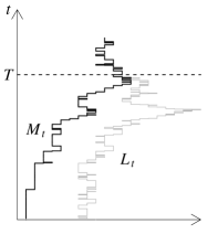
Figure 4:

(A) A realisation of the processes $({\underline{M}}_{t})_{t\geq 0}$ and $(\underline{L}_{t})_{t\geq 0}$ for the case of one colony. The joint distribution of these two processes is given in Proposition 3.1. $T$ is the first time $t$ when ${\underline{M}}_{t}={\underline{L}}_{t}$. (B) The pair $(\underline{L},\underline{M})$ has an underlying structure in terms of the particle system $\hat{\mathcal{Y}}$, where $\underline{L}$ arises as the counting process of all particles in $\hat{\mathcal{Y}}$, and $({\underline{M}}_{t})_{t\geq 0}$ is the counting process of the marked particles in $\hat{\mathcal{Y}}$.

Proposition 3.1 (An approximation of $T_{\text{fix}}$).

Let $(\underline{L}_{t},\underline{M}_{t})$, $\underline{L}_{t}=(L_{t}^{1},\dots,L_{t}^{d})$, $\underline{M}_{t}=(M_{t}^{1},\dots,M_{t}^{d})$, be defined as follows: For fixed $\iota\in\{1,\ldots,d\}$, let $\Pi_{1},\dots,\Pi_{d}$ be independent and $\text{Poi}(2\alpha\rho_{i})$-distributed, and put ${\underline{L}}_{0}=\underline{\Pi}+\underline{e}_{\iota}$, $\underline{M}_{0}=\underline{e}_{{\iota}}$. The process $(\underline{L},\underline{M})$ jumps from $(\underline{\ell},\underline{m})$ to

$$(\underline{\ell}+\underline{e}_{i},\underline{m}+\underline{e}_{i}) \text{ at rate }\alpha m_{i},$$

$$(\underline{\ell}+\underline{e}_{i},\underline{m}) \text{ at rate }\alpha(\ell_{i}-m_{i}),$$

$$(\underline{\ell}-\underline{e}_{i},\underline{m}-\underline{e}_{i}) \text{ at rate }\frac{1}{\rho_{i}}\binom{m_{i}}{2},$$

$$(\underline{\ell}-\underline{e}_{i},\underline{m}) \text{ at rate }\frac{1}{\rho_{i}}{(\ell_{i}-m_{i})}m_{i}+\frac{1}{\rho_{i}}\binom{\ell_{i}-m_{i}}{2},$$

$$(\underline{\ell}-\underline{e}_{i}+\underline{e}_{j},\underline{m}-\underline{e}_{i}+\underline{e}_{j}) \text{ at rate }\mu a(i,j)m_{i},$$

$$(\underline{\ell}-\underline{e}_{i}+\underline{e}_{j},\underline{m}) \text{ at rate }\mu a(i,j)(\ell_{i}-m_{i}).$$

Moreover, let

$$T:=\inf\{t\geq 0:\underline{M}_{t}=\underline{L}_{t}\},$$ (3.3)

and let $T_{\rm{fix}}$ be the fixation time of $\mathcal{X}^{\ast}$, where $\mathcal{X}^{\ast}$ is a solution of the SDE (2) as described in Theorem 1. Assume that the limiting distribution of $\frac{\alpha}{\log\alpha}T$ exists as $\alpha\to\infty$. Then

$$\lim_{\alpha\to\infty}\mathbf{P}_{\underline{0}}^{\iota}\Big{(}\frac{\alpha}{\log\alpha}T_{\rm{fix}}\leq t\Big{)}=\lim_{\alpha\to\infty}\mathbb{P}\Big{(}\frac{\alpha}{\log\alpha}T\leq t\Big{)},$$ (3.4)

in each continuity point of the limiting distribution function. Here, $\mu=\mu(\alpha)$ can depend on $\alpha$ in an arbitrary way.

Remark 3.2 (Existence of limiting distribution).

Our proof of Theorem 2 in Sec. 4 will reveal in particular that the limiting distribution of $\frac{\alpha}{\log\alpha}T$ exists as $\alpha\to\infty$, at least if $\mu=\mu(\alpha)$ falls in one of the three cases of Theorem 2.

3.2 The structured ancestral selection graph as a particle system

We will define a Markov process ${\mathcal{A}}=({\mathcal{A}_{r})_{r\geq 0}}$ that takes its values with probability 1 in the set of finite subsets of $\{1,\ldots,d\}\times[0,1]$. We shall refer to the elements of ${\mathcal{A}_{r}}$ as particles. For each particle $(i,u)\in{\mathcal{A}_{r}}$, we call $i$ the particle’s location and $u$ the particle’s label. Recall that we denote the probability measure that underlies ${\mathcal{A}}$ by $\mathbb{P}$. It will sometimes be convenient to annotate the configuration of locations of the initial state as a superscript of $\mathcal{A}$ or $\mathcal{Z}$. Specifically, for $\underline{k}=(k_{1},\ldots,k_{d})\in\mathbb{N}_{0}^{d}$, we put

$${\mathcal{A}}^{\underline{k}}_{0}=\bigcup_{i=1}^{d}\{(i,U_{ig}):1\leq g\leq k_{i}\},$$ (3.5)

where the $U_{ig}$ are independent and uniformly distributed on $[0,1]$.

We now specify the Markovian dynamics of ${\mathcal{A}}$ in terms of its jump kernel $\mathscr{D}^{b}$ for some migration kernel $\underline{\underline{b}}$ on $\{1,\dots,d\}$. Here we distinguish three kinds of events (see Figure LABEL:fig:split for an illustration):

• Coalescence: for all $i=1,\ldots,d$, every pair of particles in colony $i$ is replaced at rate $1/\rho_{i}$ by one particle in colony $i$ with a label that is uniformly distributed on $[0,1]$ and independent of everything else.

• Branching: for all $i=1,\ldots,d$, every particle in colony $i$ is replaced at rate $\alpha$ by two particles in colony $i$ with labels that are uniformly distributed on $[0,1]$ and independent of each other and of everything else.

• Migration: for all $i=1,\ldots,d$, every particle in colony $i$ is replaced at rate $\mu\,b(i,j)$, $j\in\{1,\ldots,d\},j\neq i$, by a particle in colony $j$ with a label that is uniformly distributed on $[0,1]$ and independent of everything else.

We will refer to ${\mathcal{A}}=({\mathcal{A}_{r}})_{r\geq 0}$ also as the structured ancestral selection graph (or ASG for short). The vector of particle numbers at time $r$ is $\underline{K}_{r}=(K_{r}(1),\ldots,K_{r}(d))$ with

$$K_{r}(i):=\#\left({\mathcal{A}_{r}}\cap(\{i\}\times[0,1])\right),\,r\geq 0,\,i=1,\ldots,d.$$ (3.6)

${\underline{K}:=}(\underline{K}_{r})_{r\geq 0}$ is a Markov process whose jump rates (based on the migration kernel $\underline{\underline{b}}$) are for $\underline{k}=(k_{1},\dots,k_{d})\in\mathbb{N}_{0}^{d}\setminus\{\underline{0}\}$ given by

$$q^{b}_{\underline{k},\underline{k}-\underline{e}_{i}} :=q_{\underline{k},\underline{k}-\underline{e}_{i}}:=\frac{1}{\rho_{i}}\binom{k_{i}}{2},$$ (3.7)

$$q^{b}_{\underline{k},\underline{k}+\underline{e}_{i}} :=q_{\underline{k},\underline{k}+\underline{e}_{i}}:=\alpha k_{i},$$

$$q^{b}_{\underline{k},\underline{k}-\underline{e}_{i}+\underline{e}_{j}} :=\mu\,b(i,j)k_{i},$$

$$q^{b}_{\underline{k},\underline{\ell}} :=q_{\underline{k},\underline{\ell}}:=0\quad\mbox{otherwise}.$$

By analogy with the notation ${\mathcal{A}^{\underline{k}}}$, we write $(\underline{K}^{\underline{k}}_{r})_{r\geq 0}$ for the process with initial state $\underline{k}$.

(A)

Coalescence

units ¡.6cm,.6cm¿ x from 0 to 6, y from -.5 to 1.5

Proof.

We will prove the duality relation

$$\pi(d\underline{z})\mathscr{D}^{b}(\underline{z},d\underline{z}^{\prime})=\pi(d\underline{z}^{\prime}){\mathscr{D}}^{a}(\underline{z}^{\prime},d\underline{z}),$$ (3.8)

which by well known results about time reversal of Markov chains in equilibrium (see e.g. Norris (1998)) proves both assertions of the Proposition at once. Since, given the particles’ locations, their labels are independent and uniformly distributed on $[0,1]$ and since this is propagated in each of the (coalescence, branching and migration) events, it will be sufficient to consider the process $\underline{K}$. Indeed, defining $q^{a}_{\underline{k},\underline{\ell}}$ as in (3.7) and putting

$$\pi_{(k_{1},\dots,k_{d})}=\frac{e^{-2\alpha}}{1-e^{-2\alpha}}\frac{(2\alpha)^{k_{1}+\cdots+k_{d}}}{k_{1}!\cdots k_{d}!}\rho_{1}^{k_{1}}\cdots\rho_{d}^{k_{d}},\quad\underline{k}\in\mathbb{N}_{0}^{d}\setminus\{\underline{0}\},$$

one readily checks for all $\underline{k}\in\mathbb{N}_{0}^{d}\setminus\{\underline{0}\}$

$$\pi_{\underline{k}}\cdot q_{\underline{k},\underline{k}-\underline{e}_{i}}=\pi_{\underline{k}-\underline{e}_{i}}\cdot q_{\underline{k}-\underline{e}_{i},\underline{k}},\quad\pi_{\underline{k}}\cdot q^{b}_{\underline{k},\underline{k}-\underline{e}_{i}+\underline{e}_{j}}=\pi_{\underline{k}-\underline{e}_{i}+\underline{e}_{j}}\cdot q^{a}_{\underline{k}-\underline{e}_{i}+\underline{e}_{j},\underline{k}}.$$

This can be summarized as

$$\pi_{\underline{k}}q^{b}_{\underline{k},\underline{\ell}}=\pi_{\underline{\ell}}q^{a}_{\underline{\ell},\underline{k}},\quad\underline{k},\underline{\ell}\in\mathbb{N}_{0}^{d}\setminus\{\underline{0}\},$$

which by definition of $\mathscr{D}^{b}$ and ${\mathscr{D}}^{a}$ lifts to (3.8), and thus proves the Proposition. ∎

3.3 Genealogical relationships in the ASG

Thanks to the labelling of the particles it makes sense to speak about genealogical relationships within ${\mathcal{A}}$. Doing so will facilitate the interpretation of the duality relationships in the proofs of Proposition 3.1 and Theorem 1.

Definition 3.3 (Connections between particles in ${\mathcal{A}}$).

Let ${\mathcal{A}}$ follow the dynamics $\mathscr{D}^{b}$ described in Section 3.2. We say that a particle $(i^{\prime},u^{\prime})$ replaces a particle $(i,u)$ if either of the following relations hold:

• there is a migration event in which $(i,u)$ is replaced by $(i^{\prime},u^{\prime})$,

• there is a coalescence event for which $(i,u)$ belongs to the pair which is replaced by $(i^{\prime},u^{\prime})$,

• there is a branching event for which $(i^{\prime},u^{\prime})$ belongs to the pair which replaces $(i,u)$.

(Note that in the 2nd and 3rd case we have necessarily $i=i^{\prime}$.) For $r,s\geq 0$ we say that two particles $(i,u)\in{\mathcal{A}_{r\wedge s}}$, $(i^{\prime},u^{\prime})\in{\mathcal{A}_{r\vee s}}$ are connected if either $(i,u)=(i^{\prime},u^{\prime})$ or there exists an $n\in\mathbb{N}$ and $(i_{0},u_{0}),\ldots,(i_{n},u_{n})$ such that $(i_{0},u_{0})=(i,u)$, $(i_{n},u_{n})=(i^{\prime},u^{\prime})$, and $(i_{\ell},u_{\ell})$ replaces $(i_{\ell-1},u_{\ell-1})$ for $\ell=1,\ldots,n$. For any subset $\mathcal{S}_{r}$ of ${\mathcal{A}_{r}}$, let

$$\mathscr{C}_{s}(\mathcal{S}_{r}):=\bigcup_{(i,u)\in\mathcal{S}_{r}}\{(i^{\prime},u^{\prime})\in{\mathcal{A}_{s}}:(i,u)\text{ and }(i^{\prime},u^{\prime})\text{ are connected}\}$$

be the collection of all those particles in ${\mathcal{A}_{s}}$ that are connected with at least one particle in $\mathcal{S}_{r}$. We briefly call $\mathscr{C}_{s}(\mathcal{S}_{r})$ the subset of ${\mathcal{A}_{s}}$ that is connected with $\mathcal{S}_{r}$.

3.4 Basic duality relationship

We recall a basic duality result for the ASG for a structured population in Lemma 3.6, as can e.g. be found in (Athreya and Swart, 2005, equation (1.5)). For this purpose we use a marking procedure of the process ${\mathcal{A}}$.

Definition 3.4 (A marking of particles).

Let $\mathcal{A}$ follow the dynamics $\mathscr{D}^{b}$ described in Section 3.2, and fix a time $\tau>0$. Take $\underline{x}=(x_{1},\ldots,x_{d})\in[0,1]^{d}$, and mark independently all particles in colony $i$ at time $\tau$ with probability $x_{i}$. Denote by

$$\mathcal{A}_{\tau}^{(\underline{x})}:=\{(i,u)\in\mathcal{A}_{\tau}:(i,u)\mbox{ is marked }\}$$

the collection of all marked particles in $\mathcal{A}_{\tau}$.

Remark 3.5 (Connectedness and marks).

In the sequel we will use the following observation: for any subset $\mathcal{S}_{0}$ of $\mathcal{A}_{0}$,

$$\mathcal{S}_{0}\cap{\mathscr{C}_{0}(\mathcal{A}_{\tau}^{(\underline{x})})}=\varnothing\,\mbox{ if and only if }\,\mathscr{C}_{\tau}(\mathcal{S}_{0})\cap{\mathcal{A}}_{\tau}^{(\underline{x})}=\varnothing.$$

For $\mathcal{S}_{0}={\mathcal{A}_{0}}$, we find that $\mathscr{C}_{0}(\mathcal{A}_{\tau}^{(\underline{x})})=\varnothing$ if and only if $\mathcal{A}_{\tau}^{(\underline{x})}=\varnothing$.
In words: no particle in $\mathcal{S}_{0}$ is marked (i.e. of “beneficial type”), if and only if no potential ancestral particle of $\mathcal{S}_{0}$ is marked.

Lemma 3.6 (Basic duality relationship).

Let $\mathcal{X}=(\underline{X}(t))_{t\geq 0}$ be the solution of (2) with $\underline{X}(0)=\underline{x}\in[0,1]^{d}$, and let $\mathcal{A}$ follow the dynamics $\mathscr{D}^{b}$. Then, for all $\underline{k}=(k_{1},\ldots,k_{d})\in\mathbb{N}_{0}^{d}$, we have, using the notation (3.1) and (3.6)

$$\mathbf{E}_{\underline{x}}[(\underline{1}-\underline{X}(\tau))^{\underline{k}}]=\mathbb{E}[(\underline{1}-\underline{x})^{\underline{K}^{\underline{k}}_{\tau}}]={\mathbb{P}({\mathcal{A}}_{\tau}^{(\underline{x})}=\varnothing|\#{\mathcal{A}}_{0}=\underline{k})}.$$ (3.9)

Proof.

The generator of the Markov process $\mathcal{X}$ is given by

$$G_{\mathcal{X}}f(\underline{x}) =\tfrac{1}{2}\sum_{j=1}^{d}\frac{1}{\rho_{i}}x_{i}(1-x_{i})\frac{\partial f^{2}(\underline{x})}{\partial^{2}x_{i}}+\alpha\sum_{i=1}^{d}x_{i}(1-x_{i})\frac{\partial f(\underline{x})}{\partial x_{i}}$$

$$\qquad\qquad\qquad\qquad\qquad\qquad\qquad+\mu\sum_{i,j=1}^{d}b(i,j)(x_{j}-x_{i})\frac{\partial f(\underline{x})}{\partial x_{i}}$$

for functions $f\in\mathcal{C}^{2}([0,1]^{d})$. Hence, for $f_{\underline{k}}(\underline{x}):=(1-\underline{x})^{\underline{k}}$ and $g_{\underline{x}}(\underline{k}):=(1-\underline{x})^{\underline{k}}$,

$$G_{\mathcal{X}}{f_{\underline{k}}(\underline{x})} =\sum_{i=1}^{d}\frac{1}{\rho_{i}}x_{i}\binom{k_{i}}{2}(1-\underline{x})^{\underline{k}-\underline{e}_{i}}+\alpha\sum_{i=1}^{d}k_{i}(-x_{i})(1-\underline{x})^{\underline{k}}$$

$$\qquad\qquad\qquad+\mu\sum_{i,j=1}^{d}b(i,j)k_{i}((1-x_{j})-(1-x_{i}))(1-\underline{x})^{\underline{k}_{i}-\underline{e}_{i}}$$

$$=\sum_{i=1}^{d}\frac{1}{\rho_{i}}\binom{k_{i}}{2}\big{(}(1-\underline{x})^{\underline{k}-\underline{e}_{i}}-(1-\underline{x})^{\underline{k}}\big{)}$$

$$\qquad\qquad\qquad+\alpha\sum_{i=1}^{d}k_{i}\big{(}(1-\underline{x})^{\underline{k}+\underline{e}_{i}}-(1-\underline{x})^{\underline{k}}\big{)}$$

$$\qquad\qquad\qquad+\mu\sum_{i,j=1}^{d}b(i,j)k_{i}\big{(}(1-\underline{x})^{\underline{k}-\underline{e}_{i}+\underline{e}_{j}}-(1-\underline{x})^{\underline{k}}\big{)}$$

$$=G_{\underline{K}}{g_{\underline{x}}(\underline{k})},$$

where $G_{\underline{K}}$ is the generator of $\underline{K}$. Now, the first equality in the duality relationship (3.9) is straightforward; see (Ethier and Kurtz, 1986, Section 4.4). The second equality in (3.9) is immediate from the definition of the marking procedure in Definition 3.4. ∎

3.5 A paintbox representation of $\underline{X}(\tau)$

Our next aim is a de Finetti–Kingman paintbox representation of the distribution of $\underline{X}(\tau)$ under $\mathbf{P}_{\underline{x}}$ in terms of the dual process $\underline{K}^{\underline{\infty}}$. In order to achieve this, we need to be able to start the ASG with infinitely many lines and define frequencies of marked particles.

Remark 3.7 (Asymptotic frequencies).

1. The process ${\mathcal{A}}$ can be started from

   $${\mathcal{A}^{\underline{\infty}}_{0}}=\bigcup_{i=1}^{d}\{(i,U_{ig})\}:1\leq g<\infty\},$$ (3.10)

   where $(U_{ig})_{i=1,\dots,d,g=1,2,\dots}$ is an independent family of uniformly distributed random variables on $[0,1]$. Indeed, the quadratic death rates of the process $\underline{K}$ (recall this process from (3.6)) ensure that the number of particles comes down from infinity. In order to see this, consider the process $(K_{r}^{1}+\cdots+K_{r}^{d})_{r\geq 0}$ and note that given $K_{r}^{1}+\cdots+K_{r}^{d}=k$ it increases at rate $\alpha k$ and its rate of decrease is minimal if colony $i$ carries $\rho_{i}k$ lines, $i=1,\dots,d$, hence is bounded from below by

   $$\sum_{i=1}^{d}\frac{1}{\rho_{i}}{{k_{i}}\choose{2}}\geq\frac{1}{2}\Bigg{(}\sum_{i=1}^{d}{k_{i}}^{2}-k\Bigg{)}\geq\frac{1}{2}\Bigg{(}\frac{1}{d}k^{2}-k\Bigg{)}\geq\frac{k(k-d)}{2d},$$ (3.11)

   where we have used the Cauchy–Schwarz inequality in the second ”$\geq$”. Using the same bounds as in Proposition 6.9 of Depperschmidt et al. (2012), we see that $\#\mathcal{A}^{\underline{\infty}}_{\varepsilon}=O(\varepsilon^{-1})$ as $\varepsilon\to 0$.

2. For $i=1,\ldots,d$, let $(J_{i1},J_{i2},\ldots):=((i,U_{i1}),(i,U_{i2}),\ldots)$ be the (numbered) collection of particles in ${\mathcal{A}_{0}^{\underline{\infty}}}$ that are located in colony $i$. Then by definition of the dynamics of ${\mathcal{A}^{\underline{\infty}}}$, the sequence

   $$(\mathbbm{1}_{\{J_{i1}\in{\mathscr{C}_{0}(\mathcal{A}_{\tau}^{(\underline{x})})}\}},\mathbbm{1}_{\{J_{i2}\in{\mathscr{C}_{0}(\mathcal{A}_{\tau}^{(\underline{x})})}\}},\ldots)$$ (3.12)

   is exchangeable. Thus, by de Finetti’s theorem, the asymptotic frequency of ones in this sequence exists a.s., which we denote by $\underline{F}^{\underline{x},\tau}=(F_{i}^{\underline{x},\tau})_{i=1,\dots,d}$ with

   $$F_{i}^{\underline{x},\tau}:=\lim_{n\to\infty}\frac{1}{n}\sum_{j=1}^{n}\mathbbm{1}_{\{J_{ij}\in\mathscr{C}_{0}(\mathcal{A}_{\tau}^{(\underline{x})})\}}$$ (3.13)

Lemma 3.8 (Asymptotic frequencies and the solution of (2)).

For $\underline{x}\in[0,1]^{d}\setminus\{\underline{0}\}$, let $\underline{F}^{\underline{x},\tau}$ be as in (3.13). Then, for the solution $\underline{X}$ of  (2) and $\tau\geq 0$,

$$\mathbb{P}(\underline{F}^{\underline{x},\tau}\in(.))=\mathbf{P}_{\underline{x}}(\underline{X}(\tau)\in(.)).$$ (3.14)

Proof.

From (3.10), for all $\underline{k}\in\mathbb{N}_{0}^{d}\setminus\{\underline{0}\}$, the process ${\mathcal{A}^{\underline{k}}}$ can be seen as embedded in ${\mathcal{A}^{\underline{\infty}}}$, if we write

$${\mathcal{A}_{0}^{\underline{k}}}:=\bigcup_{i=1}^{d}\{(i,U_{ig}):1\leq g\leq k_{i}\}\subset{\mathcal{A}^{\underline{\infty}}_{0}}.$$ (3.15)

By exchangeability of the sequence (3.12) and de Finetti’s theorem (cf. Remark 3.7) we obtain

$$\mathbb{E}[(\underline{1}-\underline{F}^{\underline{x},\tau})^{\underline{k}}]=\mathbb{P}({\mathcal{A}_{0}^{\underline{k}}}\cap{\mathscr{C}_{0}(\mathcal{A}_{\tau}^{(\underline{x})})}=\varnothing).$$ (3.16)

Since the right-hand sides of (3.16) and (3.9) are equal, we conclude from Lemma 3.6 that

$$\mathbb{E}[(\underline{1}-\underline{F}^{\underline{x},\tau})^{\underline{k}}]=\mathbf{E}_{\underline{x}}[(\underline{1}-\underline{X}(\tau))^{\underline{k}}]$$

which shows (3.14), since $\underline{k}\in\mathbb{N}_{0}^{d}\setminus\{\underline{0}\}$ was arbitrary. ∎

Under $\mathbb{P}$ we have $\underline{F}^{\underline{x},\tau}=\underline{1}$ a.s. if and only if for all $i=1,\ldots,d$ the sequences $(\mathbbm{1}_{\{J_{i1}\in{\mathscr{C}_{0}(\mathcal{A}_{\tau}^{(\underline{x})})}\}},\mathbbm{1}_{\{J_{i2}\in{\mathscr{C}_{0}(\mathcal{A}_{\tau}^{(\underline{x})})}\}},\ldots)$ consist of ones a.s. Hence the events $\{\underline{F}^{\underline{x},\tau}=\underline{1}\}$ and $\{{\mathscr{C}_{0}(\mathcal{A}_{\tau}^{(\underline{x})})}=\mathcal{A}_{0}^{\underline{\infty}}\}$ are a.s. equal under $\mathbb{P}$. A fortiori we have

$${\mathbf{P}_{\underline{x}}(T_{\rm fix}\leq\tau)}=\mathbf{P}_{\underline{x}}(\underline{X}(\tau)=1)=\mathbb{P}({\mathscr{C}_{0}(\mathcal{A}_{\tau}^{(\underline{x})})}={\mathcal{A}_{0}^{\underline{\infty}}}).$$ (3.17)

This equality allows to compute the probability of eventual fixation.

Corollary 3.9 (Eventual fixation).

The probability for eventual fixation of the beneficial type,

$$h(\underline{x}):=\mathbf{P}_{\underline{x}}(T_{\rm fix}<\infty)$$ (3.18)

can be represented as (using the notation introduced in Lemma 3.6)

$$h(\underline{x})=1-\mathbb{E}\left[(\underline{1}-\underline{x})^{\underline{\Psi}}\right],$$ (3.19)

where

$$\underline{\Psi}\in\mathbb{N}_{0}^{d}\setminus\{\underline{0}\} \alpha\underline{\rho}$$ is Poisson(2)-distributed, conditioned to be non-zero. (3.20)

In other words, $\underline{\Psi}$ counts the number of particles in colonies $1,\ldots,d$ of the Poisson point process from Proposition LABEL:lemeq. In particular, $h(\underline{x})$ is given by formula (2.4).

Proof.

Since $\mathbf{P}_{\underline{x}}(T_{\text{fix}}<\infty)=\lim_{\tau\to\infty}\mathbf{P}_{\underline{x}}(T_{\text{fix}}\leq\tau)$, we can apply the representation (3.17). We have that $\underline{K}^{\underline{\infty}}_{\tau}\xRightarrow{\tau\to\infty}\underline{\Psi}$, and the probability that $(\underline{K}^{\underline{\infty}}_{r})_{r\geq 0}$ between times $r=0$ and $r=\tau$ has a “bottleneck” at which the total number of lines equals 1 converges to one; this was called the ultimate ancestor in Krone and Neuhauser (1997). Thus, as $\tau\to\infty$, the r.h.s. of (3.17) converges to the probability that at least one particle in the configuration $\underline{\Psi}$ is marked (provided all the particles at colony $i$ are marked independently with probability $x_{i}$). This latter probability equals the r.h.s. of (3.19). To evaluate this explicitly, we write for independent $L_{i}\sim\text{Poi}(2\alpha\rho_{i})$, $i=1,\dots,d$ and $\underline{L}=(L_{1},\dots,L_{d})$, $L=L_{1}+\cdots+L_{d}$ (see Proposition LABEL:lemeq)

$$(1-e^{-2\alpha})h(\underline{x}) =(1-e^{-2\alpha})(1-\mathbb{E}[(1-\underline{x})^{\underline{\Psi}}])$$

$$=(1-e^{-2\alpha})-\mathbb{E}[(1-\underline{x})^{\underline{L}},\underline{L}\neq\underline{0}]$$

$$=(1-e^{-2\alpha})-\mathbb{E}[(1-\underline{x})^{\underline{L}}]+\mathbb{P}(L=0)$$

$$=1-\prod_{i=1}^{d}\mathbb{E}[(1-x_{i})^{L_{i}}]$$

$$=1-\prod_{i=1}^{d}e^{-2\alpha\rho_{i}}e^{2\alpha\rho_{i}(1-x_{i})}=1-e^{-2\alpha(x_{1}\rho_{1}+\cdots+x_{d}\rho_{d})},$$

i.e. we have shown (2.4). ∎

3.6 A duality conditioned on fixation

The next lemma is the analogue of Lemma 3.6 for the conditioned diffusion $\mathcal{X}^{\ast}$ in place of $\mathcal{X}$. Here, for $\underline{k}\in\mathbb{N}_{0}^{d}\setminus\{\underline{0}\}$, we will use the process $\mathcal{A}$, which follows the dynamics $\mathscr{D}^{b}$ and has the initial state $\mathcal{Y}_{0}\cup\mathcal{Z}^{\underline{k}}_{0}$, where $\mathcal{Z}^{\underline{k}}_{0}$ is as in the right hand side of (3.5) and $\mathcal{Y}_{0}$ is an equilibrium state for the dynamics $\mathscr{D}^{b}$ (as described in Proposition LABEL:lemeq) which is independent of $\mathcal{Z}^{\underline{k}}_{0}$. Note that this independence guarantees that, with probability one, all labels are distinct, and hence $\mathcal{Y}_{0}$ is a.s. disjoint from $\mathcal{Z}^{\underline{k}}_{0}$.

In terms of $\mathcal{A}$, we define two processes $\mathcal{Y}$ and $\mathcal{Z}=\mathcal{Z}^{\underline{k}}$, which follow the dynamics $\mathscr{D}^{b}$ with initial states $\mathcal{Y}_{0}$ and $\mathcal{Z}_{0}$, by setting

$$\mathcal{Z}_{s}=\mathscr{C}_{s}(\mathcal{Z}_{0}^{\underline{k}})\text{ and }\mathcal{Y}_{s}=\mathscr{C}_{s}(\mathcal{Y}_{0}),s\geq 0.$$

We emphasize that $\mathcal{Z}^{\underline{k}}\stackrel{{\scriptstyle d}}{{=}}\mathcal{A}^{\underline{k}}$ and $\mathcal{Y}\stackrel{{\scriptstyle d}}{{=}}\mathcal{A}^{\underline{\Psi}}$ due to exchangeability of particles, hence $\mathcal{Z}^{\underline{k}}$ and $\mathcal{Y}$ constitute a coupling of $\mathcal{A}^{\underline{k}}$ and $\mathcal{A}^{\underline{\Psi}}$ (with disjoint initial states).

Lemma 3.10 (Duality conditioned on fixation).

Under $\mathbf{P}_{\underline{x}}$ let $\mathcal{X}^{\ast}=(\underline{X}^{\ast}(t))_{t\geq 0}$ be the solution of (2), started in $\underline{X}^{\ast}(0)=\underline{x}$. Under $\mathbb{P}$ and for $\underline{k}\in\mathbb{N}_{0}^{d}\setminus\{\underline{0}\}$, let $\mathcal{A}$, $\mathcal{Y}$ and $\mathcal{Z}=\mathcal{Z}^{\underline{k}}$ be as described above. Then

$$\mathbf{E}_{\underline{x}}[(\underline{1}-\underline{X}^{\ast}(\tau))^{\underline{k}}] =\mathbb{P}(\mathcal{Z}_{0}^{\underline{k}}\cap\mathscr{C}_{0}({\mathcal{A}_{\tau}^{(\underline{x})}})=\varnothing\mid\mathcal{Y}_{0}\cap{\mathscr{C}_{0}(\mathcal{A}_{\tau}^{(\underline{x})})}\neq\varnothing)$$

$$=\mathbbm{P}(\mathcal{Z}_{\tau}^{\underline{k}}\cap\mathcal{A}^{(\underline{x})}_{\tau}{=\varnothing}\mid\mathcal{Y}_{\tau}\cap\mathcal{A}_{\tau}^{(\underline{x})}\neq\varnothing).$$ (3.21)

Proof.

In view of Remark 3.5 the fixation probability (3.18) can be expressed as

$$h(\underline{x})=\mathbb{P}(\mathcal{Y}_{0}\cap{\mathscr{C}_{0}(\mathcal{A}_{\tau}^{(\underline{x})})}\neq\varnothing)=\mathbb{P}(\mathcal{Y}_{\tau}\cap\mathcal{A}_{\tau}^{(\underline{x})}\neq\varnothing),\quad\tau\geq 0.$$ (3.22)

The second equality in (3.10) follows right away from Remark 3.5. To show the first equality, we set out by writing the Markovian semigroup of $\underline{X}^{\ast}$ as the $h$-transform of the semigroup of $\underline{X}$,

$$\mathbf{E}_{\underline{x}}[(\underline{1}-\underline{X}^{\ast}({\tau}))^{\underline{k}}]=\frac{\mathbf{E}_{\underline{x}}[(\underline{1}-\underline{X}({\tau}))^{\underline{k}},T_{\text{fix}}<\infty]}{\mathbf{P}_{\underline{x}}(T_{\text{fix}}<\infty)}=\frac{\mathbf{E}_{\underline{x}}[(\underline{1}-\underline{X}({\tau}))^{\underline{k}}\,h(\underline{X}({\tau})]}{h(\underline{x})}.$$ (3.23)

The numerator of the right-hand side of (3.23) equals

$$\mathbf{E}_{\underline{x}}[(\underline{1}-\underline{X}(\tau))^{\underline{k}}\, (1-\mathbb{E}[(\underline{1}-\underline{X}(\tau))^{\underline{\Psi}}])]$$

$$=\mathbf{E}_{\underline{x}}[(\underline{1}-\underline{X}(\tau))^{\underline{k}}]-\mathbb{E}\otimes\mathbf{E}_{\underline{x}}[(\underline{1}-\underline{X}(\tau))^{\underline{\Psi}+\underline{k}}].$$ (3.24)

Writing $(\underline{K}^{\underline{k}}_{r})_{r\geq 0}$, $(\underline{N}_{r})_{r\geq 0}$ and $(\underline{G}_{r})_{r\geq 0}$ for the processes of particle numbers in $\mathcal{Z}^{\underline{k}}$, $\mathcal{Y}$ and $\mathcal{A}$, respectively, we obtain from the duality relation (3.9) that

$$\mathbb{E}\otimes\mathbf{E}_{\underline{x}}[(\underline{1}-\underline{X}(\tau))^{\underline{\Psi}+\underline{k}}] =\mathbbm{E}[\mathbbm{E}[\mathbf{E}_{\underline{x}}(\underline{1}-\underline{X}(\tau))^{\underline{N}_{0}+\underline{k}}|\underline{N}_{0}]]]$$

$$=\mathbbm{E}[\mathbbm{E}[(\underline{1}-\underline{x})^{\underline{G}_{\tau}}|\underline{G}_{0}]]=\mathbb{E}[(\underline{1}-\underline{x})^{\underline{G}_{\tau}}].$$

Hence, again by the duality relation (3.9) and by Remark 3.5, the right hand side of (3.24) is equal to

$$\mathbbm{E}[(1-\underline{x})^{K^{\underline{k}}_{\tau}}]-\mathbb{E}[(\underline{1}-\underline{x})^{\underline{G}_{\tau}}] =\mathbb{P}(\mathcal{Z}^{\underline{k}}_{\tau}\cap\mathcal{A}_{\tau}^{(\underline{x})}=\varnothing)-\mathbb{P}({\mathcal{A}_{\tau}^{(\underline{x})}}=\varnothing)$$

$$=\mathbb{P}(\mathcal{Z}^{\underline{k}}_{0}\cap{\mathscr{C}_{0}(\mathcal{A}_{\tau}^{(\underline{x})})}=\varnothing)-\mathbb{P}((\mathcal{Z}^{\underline{k}}_{0}\cup\mathcal{Y}_{0})\cap{\mathscr{C}_{0}(\mathcal{A}_{\tau}^{(\underline{x})})}=\varnothing)$$

$$=\mathbb{P}(\{\mathcal{Z}_{0}^{\underline{k}}\cap{\mathscr{C}_{0}(\mathcal{A}_{\tau}^{(\underline{x})})}=\varnothing\}\cap\{\mathcal{Y}_{0}\cap{\mathscr{C}_{0}(\mathcal{A}_{\tau}^{(\underline{x})})}\neq\varnothing\}).$$

Combining this with (3.23), (3.24) and (3.22), we arrive at the first equality in (3.10). ∎

3.7 A paintbox representation for $\underline{X}^{\ast}(\tau)$

We now lift the assertion from Lemma 3.8 about the paintbox construction of $\underline{X}(\tau)$ to $\underline{X}^{\ast}(\tau)$. For this, let the process $\mathcal{A}$ follow the dynamics $\mathscr{D}^{b}$ and have the initial state $\mathcal{Y}_{0}\cup\mathcal{Z}^{\underline{\infty}}_{0}$, where $\mathcal{Z}^{\underline{\infty}}_{0}$ is as in (3.10) and $\mathcal{Y}_{0}$ is an equilibrium state for the dynamics $\mathscr{D}^{{b}}$ (as described in Proposition LABEL:lemeq) which is independent of $\mathcal{Z}^{\underline{\infty}}_{0}$. Recall from (3.13). the definition of the asymptotic frequencies $\underline{F}^{\underline{x},\tau}=(F_{i}^{\underline{x},\tau})_{i=1,\dots,d}$ of ${\mathscr{C}_{0}(\mathcal{A}_{\tau}^{(\underline{x})})}$ within $\mathcal{A}_{0}$.

Lemma 3.11 (A paintbox for $\underline{X}^{\ast}(\tau)$).

Under $\mathbf{P}_{\underline{x}}$ let $\mathcal{X}^{\ast}=(\underline{X}^{\ast}(t))_{t\geq 0}$ be the solution of (2), started in $\underline{X}^{\ast}(0)=\underline{x}$. Under $\mathbb{P}$, let the process $\mathcal{A}$ and the frequencies $\underline{F}^{\underline{x},\tau}$ be as above. Then,

$$\mathbf{P}_{\underline{x}}(\underline{X}^{\ast}(\tau)\in(.))=\mathbb{P}(\underline{F}^{\underline{x},\tau}\in(.)\mid\mathcal{Y}_{\tau}\cap\mathcal{A}_{\tau}^{(\underline{x})}\neq\varnothing).$$ (3.25)

Proof.

For $\mathcal{Z}_{0}^{\underline{\infty}}=\{J_{ig}:=(i,U_{ig}):i=1,...,d,g=1,2,...\}$, we observe that the sequence (3.12) is exchangeable under the measure $\mathbb{P}(\cdot\mid\mathcal{Y}_{\tau}\cap\mathcal{A}_{\tau}^{(\underline{x})}\neq\varnothing)$, which guarantees the a.s. existence of $\underline{F}^{\underline{x},\tau}$. We now parallel the argument in the proof of Lemma 3.8:
For each $\underline{k}\in\mathbb{N}_{0}^{d}\setminus\{\underline{0}\}$, with $\mathcal{Z}^{\underline{k}}_{0}$ is as in the right hand side of (3.5), we have because of exchangeability

$$\mathbb{E}[(\underline{1}-\underline{F}^{\underline{x},\tau})^{\underline{k}}\mid\mathcal{Y}_{\tau}\cap\mathcal{A}_{\tau}^{(\underline{x})}\neq\varnothing]=\mathbb{P}(\mathcal{Z}_{0}^{\underline{k}}\cap{\mathscr{C}_{0}(\mathcal{A}_{\tau}^{(\underline{x})})}=\varnothing\mid\mathcal{Y}_{\tau}\cap\mathcal{A}_{\tau}^{(\underline{x})}\neq\varnothing).$$

Combining this with Lemma 3.10, and since $\underline{k}$ was arbitrary, we obtain the assertion. ∎

We are interested in the limit of (3.25) as $\underline{x}=\underline{x}(\varepsilon)\sim\varepsilon\underline{e}_{\iota}$ and $\varepsilon\to 0$ for a fixed $\iota\in\{1,\ldots,d\}$. For brevity we write

$$\mathbb{P}^{\underline{x},\tau}(\cdot):=\mathbb{P}(\cdot\mid\mathcal{Y}_{\tau}\cap\mathcal{A}_{\tau}^{(\underline{x})}\neq\varnothing).$$ (3.26)

Remark 3.12 (Limit of small frequencies).

Let $\mathscr{P}$ be a Poisson point process on $\{1,\ldots,d\}\times[0,1]$ with intensity measure $2\alpha\underline{\rho}\otimes\lambda$. (Compare with Proposition LABEL:lemeq.) For $\iota\in\{1,\ldots,d\}$ and $\underline{x}=\underline{x}(\varepsilon)=\varepsilon\underline{e}_{\iota}$, the conditional distribution of $(\mathcal{Y}_{\tau},\mathcal{Y}_{\tau}\cap\mathcal{A}_{\tau}^{(\underline{x}(\varepsilon))})$ given $\{\mathcal{Y}_{\tau}\cap\mathcal{A}_{\tau}^{(\underline{x}(\varepsilon))}\neq\varnothing\}$ converges, as $\varepsilon\to 0$, to the distribution of $(\mathscr{P}^{(\iota)},\{(\iota,U)\})$, with $\mathscr{P}^{(\iota)}:=\mathscr{P}\cup\{(\iota,U)\}$, and $U$ independent of $\mathscr{P}$ and uniformly distributed on $[0,1]$. In particular, under the limit of $\mathbb{P}^{\varepsilon\underline{e}_{\iota},\tau}$ as $\varepsilon\to 0$, with probability $1$ there is exactly one marked particle in $\mathcal{Y}_{\tau}$, with the location of this particle being $\iota$. Indeed, (using the same notation as in the proof of Corollary 3.9),

$$\lim_{\varepsilon\to 0}\mathbb{P}^{\underline{x}(\varepsilon),\tau}(\#(\mathcal{Y}_{\tau}{\cap(\{\iota\}\times[0,1])})=k) =\lim_{\varepsilon\to 0}\frac{e^{-2\alpha\rho_{\iota}}(2\alpha\rho_{\iota})^{k}(1-(1-\varepsilon)^{k})/k!}{1-\sum_{\ell=0}^{\infty}e^{-2\alpha\rho_{\iota}}(2\alpha\rho_{\iota})^{\ell}(1-\varepsilon)^{\ell}/\ell!}$$ (3.27)

$$=\lim_{\varepsilon\to 0}\frac{e^{-2\alpha\rho_{\iota}}(2\alpha\rho_{\iota})^{k}k\varepsilon/k!}{1-e^{-2\alpha\rho_{\iota}\varepsilon}}$$

$$=e^{-2\alpha\rho_{\iota}}\frac{(2\alpha\rho_{\iota})^{k-1}}{(k-1)!},$$

the weight of a Poisson($2\alpha\rho_{\iota}$)-distribution at $k-1$. A similar calculation shows that this also equals the limit of $\mathbb{P}^{\underline{x}(\varepsilon),\tau}(\#(\mathcal{Y}_{\tau}{\cap(\{\iota\}\times[0,1])})=k,\#\mathcal{Y}_{\tau}\cap\mathcal{A}_{\tau}^{(\underline{x})}=1)$ as $\varepsilon\to 0$, explaining the additional particle $(\iota,U)$ in $\mathcal{Y}_{\tau}$ under $\mathbb{P}^{\iota,\tau}$.

Definition 3.13 (The process $\mathcal{A}$ with small marking probability).

ttt

• The weak limit of $\mathbb{P}^{\varepsilon\underline{e}_{\iota},\tau}(\mathcal{A}\in(.))$ as $\varepsilon\to 0$ will be denoted by

  $$\mathbb{P}^{\iota,\tau}(\mathcal{A}\in(.)).$$

  From the previous remark, under $\mathbb{P}^{\iota,\tau}$, there is a.s. exactly one marked particle in $\mathcal{Y}_{\tau}$, with the location of this particle being $\iota$. This particle will be denoted by $\bullet$.

• For each colony $i$, consider the configuration $\mathscr{C}_{0}(\{\bullet\})\cap\mathcal{Z}_{0}^{\underline{\infty}}{\cap(\{i\}\times[0,1])}$, i.e. the configuration of all particles in $\mathcal{Z}_{0}^{\underline{\infty}}$ that are located in colony $i$ and are connected with $\{\bullet\}$. By exchangeablity, the relative frequency of this configuration within $\mathcal{Z}_{0}^{\underline{\infty}}{\cap(\{i\}\times[0,1])}$ exists, $i=1,\ldots,d$, cf. Remark 3.7.2. As before, we denote the vector of these relative frequencies by $\underline{F}^{\iota,\tau}:=(F^{\iota,\tau}_{1},\dots,F^{\iota,\tau}_{d})$.

Corollary 3.14 (Entrance laws for (2)).

There exists a weak limit of the distribution of $\mathcal{X}^{\ast}$ under $\mathbf{P}_{\varepsilon\underline{e}_{\iota}}$ as $\varepsilon\to 0$, which we denote by $\mathbf{P}_{\underline{0}}^{\iota}(\mathcal{X}^{\ast}\in(.))$. In particular, $((\underline{X}^{\ast}_{t})_{t>0},\mathbf{P}_{\underline{0}}^{\iota})$ defines an entrance law from $\underline{0}$ for the dynamics (2).

Proof.

As a consequence of (3.25) and the reasoning in Remark 3.12 we have

$$\mathbf{P}_{\varepsilon\underline{e}_{\iota}}(\underline{X}^{\ast}(\tau)\in(.))=\mathbb{P}^{\varepsilon\underline{e}_{\iota},\tau}(\underline{F}^{\varepsilon\underline{e}_{\iota},\tau}\in(.))\xrightarrow{\varepsilon\to 0}\mathbb{P}^{\iota,\tau}(\underline{F}^{\iota,\tau}\in(.)).$$ (3.28)

Together with the Markov property, this shows that there exists a weak limit of the distribution of $\mathcal{X}^{\ast}$ under $\mathbf{P}_{\varepsilon\underline{e}_{\iota}}$ as $\varepsilon\to 0$. Hence the result follows. ∎

Remark 3.15 (Asymptotic expected frequencies).

For the asymptotic frequencies, we have that $\rho_{\iota}\mathbb{E}^{\iota,t}[F_{j}^{\iota,t}]/t\xrightarrow{t\to 0}\delta_{\iota j}$. Indeed, $\mathbb{E}^{\iota,t}[F_{j}^{\iota,t}]$ is the probability that a particle from $\mathcal{Z}^{{\underline{\infty}}}_{0}$ located on colony $j$ belongs to $\mathscr{C}_{0}(\{\bullet\})$. In order for the particle to be connected to $\bullet$, a coalescence event within time $t$ must occur. For small $t$, and up to linear order in $t$, this can only happen if the particle is located on the same colony, i.e. $\iota=j$. In this case, since the coalescence rate on colony $\iota$ is $1/\rho_{\iota}$, the result follows.

Remark 3.16 (A correction of Pfaffelhuber and Pokalyuk (2013)).

In Pfaffelhuber and Pokalyuk (2013) the case of a single colony ($d=1$) is studied. Lemma 2.4 of Pfaffelhuber and Pokalyuk (2013) can be seen as an analogue of our Lemma 3.11 (together with Remark 3.12). However, Lemma 2.4 of Pfaffelhuber and Pokalyuk (2013) neglects the effect which the conditioning on the event $\{\mathcal{Y}_{\tau}\cap\mathcal{A}_{\tau}^{(\underline{x})}\neq\varnothing\}$ has on the distribution of   $\underline{\Psi}$, and works right away with the time-reversal of $\mathcal{Y}$ in equilibrium. Our analysis shows that, in spite of this imprecision, the conclusions of the main results of Pfaffelhuber and Pokalyuk (2013) remain true.

As a consequence of (3.25) and (3.28) we obtain

$$\mathbf{P}^{\iota}_{\underline{0}}(T_{\rm fix}\leq\tau)=\mathbf{P}^{\iota}_{\underline{0}}(\underline{X}^{\ast}(\tau)=1)=\mathbb{P}^{\iota,\tau}(\mathcal{Z}_{0}^{\underline{\infty}}\subseteq\mathscr{C}_{0}(\{\bullet\}).$$ (3.29)

3.8 Proof of Proposition 3.1

From (3.29) we now derive a result on how to approximate $T_{\rm fix}$ as $\alpha\to\infty$. The idea is that in this limit the time which it takes for $\mathcal{Z}^{\underline{\infty}}$ to coalesce with $\mathcal{Y}$ is essentially negligible on the $\frac{\log\alpha}{\alpha}$-timescale. This is captured by the following lemma, whose proof we defer to the end of the section.

Lemma 3.17 (Approximating $T_{\rm fix}$).

For $\delta,\tau>0$, let $\delta_{\alpha}:=\delta\frac{\log\alpha}{\alpha}$ and $\tau_{\alpha}:=\tau\frac{\log\alpha}{\alpha}$, and let $\bullet$ be as in Definition 3.13. Then,

$$\mathbb{P}^{\iota,\tau_{\alpha}}(\mathcal{Z}_{0}^{\underline{\infty}}\subseteq\mathscr{C}_{0}(\{\bullet\}))\leq\mathbb{P}^{\iota,\tau_{\alpha}}(\mathcal{Y}_{0}\subseteq\mathscr{C}_{0}(\{\bullet\}))\mbox{ for all }\alpha>0,$$ (3.30)

$$\liminf_{\alpha\to\infty}\mathbb{P}^{\iota,\tau_{\alpha}}(\mathcal{Y}_{0}\subseteq\mathscr{C}_{0}(\{\bullet\}))\leq\liminf_{\alpha\to\infty}\mathbb{P}^{\iota,\tau_{\alpha}+\delta_{\alpha}}(\mathcal{Z}_{0}^{\underline{\infty}}\subseteq\mathscr{C}_{0}(\{\bullet\})).$$ (3.31)

The next corollary follows by combining (3.29) and Lemma 3.17.

Corollary 3.18.

For $\alpha>0$ let $S_{\alpha}$ be a random variable with distribution function $\tau\mapsto\mathbb{P}^{\iota,\tau_{\alpha}}(\mathcal{Y}_{0}\subseteq\mathscr{C}_{0}(\{\bullet\}))$, where $\tau_{\alpha}=\tau\frac{\log\alpha}{\alpha}$. (In the subsequent proof of Proposition 3.1 we will see that $S_{\alpha}$ has a natural interpretation as the rescaled fixation time of $\bullet$ in the time-reversal of $\mathcal{Y}$.) If $S_{\alpha}$ converges in distribution as $\alpha\to\infty$ and if $\tau$ is a point of continuity of the limiting distribution function, we have

$$\lim_{\alpha\to\infty}\mathbf{P}^{\iota}_{\underline{0}}(T_{\rm fix}\leq\tau_{\alpha})=\lim_{\alpha\to\infty}\mathbb{P}^{\iota,\tau_{\alpha}}(\mathcal{Y}_{0}\subseteq\mathscr{C}_{0}(\{\bullet\})).$$ (3.32)

Proof.

The limit in the right hand side exists by assumption. If $\tau-\delta$ is a continuity point of the limiting distribution function $F$, then we have by (3.31) (with $\tau$ replaced by $\tau-\delta$) and again abbreviating $\delta_{\alpha}=\delta\frac{\log\alpha}{\alpha}$

$$\lim_{\alpha\to\infty}\mathbb{P}^{\iota,\tau_{\alpha}-\delta_{\alpha}}(\mathcal{Y}_{0}\subseteq\mathscr{C}_{0}(\{\bullet\}))\leq\liminf_{\alpha\to\infty}\mathbb{P}^{\iota,\tau_{\alpha}}(\mathcal{Z}_{0}^{\underline{\infty}}\subseteq\mathscr{C}_{0}(\{\bullet\})).$$

Hence, working along a sequence of continuity points $\tau-\delta$ of $F$ with $\delta\downarrow 0$, we have

$$\lim_{\alpha\to\infty}\mathbb{P}^{\iota,\tau_{\alpha}}(\mathcal{Y}_{0}\subseteq\mathscr{C}_{0}(\{\bullet\})) =\lim_{\delta\to 0}\lim_{\alpha\to\infty}\mathbb{P}^{\iota,\tau_{\alpha}-\delta_{\alpha}}(\mathcal{Y}_{0}\subseteq\mathscr{C}_{0}(\{\bullet\}))$$

$$\leq\liminf_{\alpha\to\infty}\mathbb{P}^{\iota,\tau_{\alpha}}(\mathcal{Z}_{0}^{\underline{\infty}}\subseteq\mathscr{C}_{0}(\{\bullet\}))=\liminf_{\alpha\to\infty}\mathbf{P}^{\iota}_{\underline{0}}(T_{\rm fix}\leq\tau_{\alpha})$$

$$\leq\limsup_{\alpha\to\infty}\mathbf{P}^{\iota}_{\underline{0}}(T_{\rm fix}\leq\tau_{\alpha})=\limsup_{\alpha\to\infty}\mathbb{P}^{\iota,\tau_{\alpha}}(\mathcal{Z}_{0}^{\underline{\infty}}\subseteq\mathscr{C}_{0}(\{\bullet\}))$$

$$\leq\lim_{\alpha\to\infty}\mathbb{P}^{\iota,\tau_{\alpha}}(\mathcal{Y}_{0}\subseteq\mathscr{C}_{0}(\{\bullet\})).$$

∎

The preceding corollary shows that, in order to study the asymptotic distribution of $T_{\rm fix}$ on the $\frac{\log\alpha}{\alpha}$-timescale, it suffices to analyse the asymptotics of the percolation probabilities of the marked particles within the equilibrium ASG under the (conditional) probability $\mathbb{P}^{\iota,\tau_{\alpha}}$. As already explained in Sec. 3.1, the link to Proposition 3.1 is now given by a time reversal argument.

Proof of Proposition 3.1.

In view of (3.32), we are done once we show that, for $\tau>0$,

$$\mathbb{P}\big{(}T\leq\tau\big{)}=\mathbb{P}^{\iota,\tau}(\mathscr{C}_{0}(\{\bullet\})\supseteq\mathcal{Y}_{0}),$$ (3.33)

where $T$ is defined in (3.3). For this, we bring the time reversal $\widehat{\mathcal{Y}}$ of $\mathcal{Y}=(\mathcal{Y}_{r})_{0\leq r\leq\tau}$ into play, which is defined by

$$\widehat{\mathcal{Y}}_{s}:={\mathcal{Y}}_{\tau-s},\quad 0\leq s\leq\tau.$$

Analogously, we define $\widehat{\mathscr{C}}_{s}(\{\bullet\}):={\mathscr{C}}_{\tau-s}(\{\bullet\}).$ Then, our assertion (3.33) is equivalent to

$$\mathbb{P}\big{(}T\leq\tau\big{)}=\mathbb{P}^{\iota,\tau}(\widehat{\mathscr{C}}_{\tau}(\{\bullet\})\supseteq\widehat{\mathcal{Y}}_{\tau}).$$ (3.34)

We recall that the dynamics of $\widehat{\mathcal{Y}}$ in equilibrium is given by $\mathscr{D}^{a}$; see Proposition LABEL:lemeq. While for $\mathcal{Y}$ the conditioning (3.26) is at the terminal time $\tau$ (and thus modifies the dynamics $\mathscr{D}$), the same conditioning expressed for $\widehat{\mathcal{Y}}$ happens at the initial time $0$ and thus does effect the initial state but not the dynamics $\mathscr{D}^{a}$. The distribution of $\hat{\mathcal{Y}}_{0}$ which results from this conditioning is described in Remark 3.12. Thus we observe that under $\mathbb{P}^{\iota,\tau}$, the time-reversed process $\widehat{\mathcal{Y}}$ follows the dynamics $\mathscr{D}^{a}$ and has initial state $\widehat{\mathcal{Y}}_{0}=\mathscr{P}^{(\iota)}=\mathscr{P}\cup\{(\iota,U)\}$, with $\mathscr{P}$ defined in Remark 3.12 and $\bullet:=(\iota,U)$.

We now put for $i=1,\ldots,d$ and $t\geq 0$

$$\widehat{N}^{i}_{t}:=\#\left(\widehat{\mathcal{Y}}_{t}\cap(\{i\}\times[0,1])\right),\quad\widehat{H}^{i}_{t}:=\#\left(\widehat{\mathscr{C}}_{t}(\{\bullet\})\cap(\{i\}\times[0,1])\right).$$ (3.35)

Under $\mathbb{P}^{\iota,\tau}$ the process $(\widehat{\underline{N}}_{t},\widehat{\underline{H}}_{t})_{0\leq t\leq\tau}$ with $\widehat{\underline{N}}_{t}=({\widehat{N}}^{1}_{t},\dots,{\widehat{N}}^{d}_{t})$ and $\widehat{\underline{H}}_{t}=(\widehat{H}^{1}_{t},\dots,\widehat{H}^{d}_{t})$, then has the same law as the process $({\underline{L}}_{t},{\underline{M}}_{t})_{0\leq t\leq\tau}$ defined in Proposition 3.1. In particular, (3.34) is shown.

∎

We prepare the proof of Lemma 3.17 by two estimates and include their (simple) proofs for convenience.

Remark 3.19 (Comparing $\underline{\Pi}$ and $\underline{\Pi}+\underline{e}_{\iota}$).

Recall that $\underline{\Pi}=(\Pi_{1},...,\Pi_{d})$ is distributed according to $d$ independent Poisson distributions, where $\Pi_{i}\sim\text{Poi}(2\alpha\rho_{i})$. As above, $\underline{\Psi}$ is distributed as $\underline{\Pi}$, conditioned to be positive (compare with (3.20)) and $\underline{\Pi}+\underline{e}_{\iota}$ is as in Proposition 3.1. Then, ($d_{TV}$ denoting the total variation distance)

$$d_{\text{TV}}(\underline{\Pi},\underline{\Psi}) =o(1),$$ (3.36)

$$d_{\text{TV}}(\underline{\Pi},\underline{\Pi}+\underline{e}_{\iota}) =o(1)$$

as $\alpha\to\infty$.
Indeed: The first result is immediate since $\mathbb{P}[\underline{\Pi}=0]=e^{-2\alpha}$. For the second result, by a second moment calculation, we have that $\Pi_{\iota}/(2\alpha\rho_{\iota})\xrightarrow{\alpha\to\infty}1$ in $L^{2}$ and therefore, as $\alpha\to\infty$,

$$d_{\text{TV}}(\underline{\Pi},\underline{\Pi}+\underline{e}_{\iota}) =e^{-2\alpha\rho_{\iota}}\sum_{k=1}^{\infty}\Big{|}\frac{(2\alpha\rho_{\iota})^{k}}{k!}-\frac{(2\alpha\rho_{\iota})^{k-1}}{(k-1)!}\Big{|}+o(1)$$

$$=e^{-2\alpha\rho_{\iota}}\sum_{k=1}^{\infty}\frac{(2\alpha\rho_{\iota})^{k}}{k!}\Big{|}1-\frac{k}{2\alpha\rho_{\iota}}\Big{|}+o(1)$$

$$=\mathbb{E}\Big{[}\Big{|}1-\frac{\Pi_{\iota}}{2\alpha\rho_{\iota}}\Big{|}\Big{]}+o(1)=o(1).$$

We are now ready for the

Proof of Lemma 3.17.

For proving (3.30) it suffices to show that, for each ${\alpha~{}>0}$, $\mathbb{P}^{\iota,\tau_{\alpha}}((I,U)\notin\mathscr{C}_{0}(\{\bullet\}),\mathcal{Z}_{0}^{\underline{\infty}}\subseteq\mathscr{C}_{0}(\{\bullet\}))=0$ for a particle $(I,U)$ taken uniformly from $\mathcal{Y}_{0}$. To show this equality, we will prove that for all $i=1,\ldots,d$

$$\mathbb{P}^{\iota,\tau_{\alpha}}((I,U)\notin\mathscr{C}_{0}(\{\bullet\}),\mathcal{Z}_{0}^{\underline{\infty}}\subseteq\mathscr{C}_{0}(\{\bullet\}),I=i\})=0.$$ (3.37)

We write $\mathbf{p}:=(I,U)$, and note that

$$R_{\mathbf{p}}:=\inf\{r>0:\mathscr{C}_{r}(\{\mathbf{p}\})\not\subseteq\{i\}\times[0,1]\}>0\quad\mathbb{P}^{\iota,\tau_{\alpha}}\mbox{ a.s. }$$

The idea is now that with probability 1 we will find particles in $\mathcal{Z}$ which coalesce with $\bigcup_{r\geq 0}\mathscr{C}_{r}(\{\mathbf{p}\})$, withouth being affected by an earlier branching or coalescence with $\mathcal{Y}\setminus\bigcup_{r\geq 0}\mathscr{C}_{r}(\{\mathbf{p}\})$, and hence on the event $\{\mathbf{p}\notin\mathscr{C}_{0}(\{\bullet\})\}$ never connect to the particle $\bullet$. In order to achieve this, we recall that under $\mathbb{P}^{\iota,\tau_{\alpha}}$ the dynamics of $\mathcal{Z}$ is given by $\mathscr{D}^{b}$, and this also applies conditional under $\mathcal{Y}$ for the particles in $\mathcal{Z}$ up to the time of their possible coalescence with particles in $\mathcal{Y}$.

We now consider the subsystem of particles in $\mathcal{Z}$ which initiates from all those $\mathcal{Z}$ particles that are located in colony $i$ at time $0$, and remove from it all those particles that undergo a migration or a branching event, or coalesce with some particle in $\mathcal{Y}_{r}\setminus\mathscr{C}_{r}(\mathbf{p})$ at some time $r\geq 0$. The system of particles of $\mathcal{Z}$ at time $r$ which remain after this pruning (and all of which are located in colony $i$ by construction) will be denoted by $\mathcal{Z}^{(i)}_{r}$.

Given $\mathcal{Y}$, the process $(\#\mathcal{Z}^{(i)}_{r})$ is up to time $R_{\mathbf{p}}$ stochastically bounded from below by a death process $(K_{r})_{{r\geq 0}}$ entering from infinity with death rate $\frac{1}{\rho_{i}}\binom{k}{2}+(\alpha+\mu\sum_{j\neq i}b(i,j)+M)k$, where $M:=\max\{\#(Y_{r}{\cap}(\{i\}\times[0,1])):0\leq r\leq R_{\mathbf{p}}\}$. Hence, the essentially quadratic death rate guarantees that for any $c>0$ $\lim_{\varepsilon\rightarrow 0}\int_{\varepsilon}^{c}K_{r}dr=\infty$ a.s. Indeed, $\rho_{i}rK_{r}\xrightarrow{r\to 0}2$ a.s. by a second moment calculation, and $K_{r}\approx\frac{2}{\rho_{i}r}$ is not integrable at $r=0$. Consequently, also $\lim_{\varepsilon\to 0}\int_{\varepsilon}^{c}\#\mathcal{Z}^{(i)}_{r}dr=\infty$ a.s., and thus with probability 1 there will be a coalescence between $\mathcal{Z}^{(i)}_{r}$ and $\mathscr{C}_{r}(\{\mathbf{p}\})$ for some $r<R_{\mathbf{p}}$.

Since on the event $\{\mathbf{p}\notin\mathscr{C}_{0}(\{\bullet\})\}$ the set $\mathscr{C}_{r}(\{\mathbf{p}\})$ is contained in the complement of $\mathscr{C}_{r}(\{\bullet\})$, we conclude the existence of particles in $\mathcal{Z}^{(i)}_{0}$ (and hence in $\mathcal{Z}_{0}^{\underline{\infty}}$) that belong to the complement of $\mathscr{C}_{0}(\{\bullet\})$. This shows (3.37).

To prove (3.31), we first note that the particle $\bullet$ specified in Definition 3.13 is (because of the random marking) a uniform choice from the particles in $\mathcal{Y}_{\tau_{\alpha}}\cap(\{\iota\}\times[0,1])$ under $\mathbb{P}^{\iota,\tau_{\alpha}}$, and a uniform choice from the particles in $\mathcal{Y}_{\tau_{\alpha}+\delta_{\alpha}}\cap(\{\iota\}\times[0,1])$ under $\mathbb{P}^{\iota,\tau_{\alpha}+\delta_{\alpha}}$.

However, as noted already after formula (3.34), the conditioning at time $\tau_{\alpha}$, which is inherent in $\mathbb{P}^{\iota,\tau_{\alpha}}$, destroys the time-homogeneity of the dynamics of $\mathcal{Y}$ between times $0$ and ${\tau_{\alpha}}$; consequently, under $\mathbb{P}^{\iota,\tau_{\alpha}}$ the marking probabilities in $\mathcal{Z}_{0}^{\underline{\infty}}$ will be different from those in $\mathcal{Y}_{0}$. In order to account for this, the strategy of our proof will be to define under the unconditioned probability measure $\mathbb{P}$ particles $\circ$ and $\circ^{\prime}$ whose distributions will turn out to be close in variation distance to that of $\bullet$ under $\mathbb{P}^{\iota,\tau_{\alpha}}$ and under $\mathbb{P}^{\iota,\tau_{\alpha}+\delta_{\alpha}}$, respectively, and which lead to the same marking probabilities in $\mathcal{Y}_{0}$ and $\mathcal{Z}_{0}^{\underline{\infty}}$.

To be specific, let $\circ$ result from a uniform pick from $(\mathcal{Y}_{\tau_{\alpha}}\cup\mathcal{Z}^{\underline{\infty}}_{\tau_{\alpha}})\cap(\{\iota\}\times[0,1])$ provided that this set is not empty; otherwise we pick $\circ$ uniformly from $\mathcal{Y}_{\tau_{\alpha}}\cup\mathcal{Z}^{\underline{\infty}}_{\tau_{\alpha}}$. Similarly, we pick $\circ^{\prime}$ uniformly from $(\mathcal{Y}_{\tau_{\alpha}+\delta_{\alpha}}\cup\mathcal{Z}^{\underline{\infty}}_{\tau_{\alpha}+\delta_{\alpha}})\cap(\{\iota\}\times[0,1])$ provided that this set is not empty; otherwise we pick $\circ^{\prime}$ uniformly from $\mathcal{Y}_{\tau_{\alpha}+\delta_{\alpha}}\cup\mathcal{Z}^{\underline{\infty}}_{\tau_{\alpha}+\delta_{\alpha}}$.

This construction immediately implies that for any fixed $i=1,...,d$, the family of events $(\{(i,U_{ig})\in\mathscr{C}_{0}(\circ)\})_{(i,U_{ig})\in\mathcal{Y}_{0}\cup\mathcal{Z}^{\underline{\infty}}_{0}}$, is exchangeable conditional under $\mathcal{Y}_{0}\cup\mathcal{Z}^{\underline{\infty}}_{0}$. We will show five properties ((A)-(E)) of the joint distribution of $\mathcal{A}$, $\mathcal{Y}$, $\mathcal{Z}^{\underline{\infty}}$ and $\circ$, proceeding in two main steps proving first (A) and then (B)-(E).
(A) the total variation distance between the distribution of $(\mathcal{A}_{t},\mathcal{Y}_{t},\mathcal{Z}^{\underline{\infty}}_{t},\circ)_{0\leq t\leq\tau_{\alpha}}$ under $\mathbb{P}$ and the distribution of $(\mathcal{A}_{t},\mathcal{Y}_{t},\mathcal{Z}^{\underline{\infty}}_{t},\bullet)_{0\leq t\leq\tau_{\alpha}}$ under $\mathbb{P}^{\iota,\tau_{\alpha}}$ converges to $0$ as $\alpha\to\infty$. Likewise, the total variation distance between the distribution of $(\mathcal{A}_{t},\mathcal{Y}_{t},\mathcal{Z}^{\underline{\infty}}_{t},\circ^{\prime})_{0\leq t\leq\tau_{\alpha}+\delta_{\alpha}}$ under $\mathbb{P}$ and the distribution of $(\mathcal{A}_{t},\mathcal{Y}_{t},\mathcal{Z}^{\underline{\infty}}_{t},\bullet)_{0\leq t\leq\tau_{\alpha}+\delta_{\alpha}}$ under $\mathbb{P}^{\iota,\tau_{\alpha}+\delta_{\alpha}}$ converges to $0$ as $\alpha\to\infty$.

Having achieved this, we will construct a process $({\mathcal{Z}}^{\prime}_{r})_{0\leq r\leq\delta_{\alpha}}$ under $\mathbb{P}$ with the following properties:
(B) $\mathcal{Z}^{\prime}_{r}\subseteq\mathcal{Z}^{\underline{\infty}}_{r}$ for all $r\in[0,\delta_{\alpha}]$,
(C) $\{\mathcal{Z}^{\prime}_{\delta_{\alpha}}\subseteq\mathscr{C}_{\delta_{\alpha}}(\circ^{\prime})\}\subseteq\{\mathcal{Z}^{\underline{\infty}}_{0}\subseteq\mathscr{C}_{0}(\circ^{\prime})\};$
(D) for any $i=1,...,d$, $\mathcal{Z}^{\prime}_{\delta_{\alpha}}(\{i\}\times[0,1])={\mathcal{O}(\alpha/\log(\alpha)})$ with high probability as $\alpha\to\infty$,
(E) for any $i=1,...,d$, the family of events $(\{(i,U_{ig})\in\mathscr{C}_{\delta_{\alpha}}(\circ^{\prime})\})_{(i,U_{ig})\in\mathcal{Y}_{\delta_{\alpha}}\cup{\mathcal{Z}^{\prime}_{\delta_{\alpha}}}}$ is exchangeable conditional under $\mathcal{Y}_{\delta_{\alpha}}\cup\mathcal{Z}^{\prime}_{\delta_{\alpha}}$.

The proof of the first assertion of (A) will be achieved in several steps.
(i) We first note that because of Remark 3.19 the total variation distance between the distributions of $\mathcal{Y}_{\tau_{\alpha}}$ under $\mathbb{P}^{\iota,\tau_{\alpha}}$ and under $\mathbb{P}$ converges to $0$ as $\alpha\to\infty$.
(ii) Now a crucial observation is that the time-reversed dynamics of $(\mathcal{Y}_{t})_{0\leq t\leq\tau_{\alpha}}$ under $\mathbb{P}$ and under $\mathbb{P}^{\iota,\tau_{\alpha}}$ both are given by the dual jump kernel ${\mathscr{D}}^{a}$. Consequently, the conditional distribution of $(\mathcal{Y}_{t})_{0\leq t\leq\tau_{\alpha}}$ given $\mathcal{Y}_{\tau_{\alpha}}$ under $\mathbb{P}^{\iota,\tau_{\alpha}}$ equals that under $\mathbb{P}$. This shows that the variational distance between the distributions of $(\mathcal{Y}_{t})_{0\leq t\leq\tau_{\alpha}}$ under $\mathbb{P}^{\iota,\tau_{\alpha}}$ and under $\mathbb{P}$ equals the variational distance between the distributions of $\mathcal{Y}_{\tau_{\alpha}}$ under $\mathbb{P}^{\iota,\tau_{\alpha}}$ and under $\mathbb{P}$.
(iii) Next note that the conditional distribution of $(\mathcal{A}_{t},\mathcal{Y}_{t},\mathcal{Z}^{\underline{\infty}}_{t})_{0\leq t\leq\tau_{\alpha}}$ given $(\mathcal{Y}_{t})_{0\leq t\leq\tau_{\alpha}}$ under $\mathbb{P}^{\iota,\tau_{\alpha}}$ equals that under $\mathbb{P}$. Hence the variational distance between the distributions of $(\mathcal{A}_{t},\mathcal{Y}_{t},\mathcal{Z}^{\underline{\infty}}_{t})_{0\leq t\leq\tau_{\alpha}}$ under $\mathbb{P}^{\iota,\tau_{\alpha}}$ and under $\mathbb{P}$ equals the variational distance between the distributions of $(\mathcal{Y}_{t})_{0\leq t\leq\tau_{\alpha}}$ under $\mathbb{P}^{\iota,\tau_{\alpha}}$ and under $\mathbb{P}$.
(iv) Combining (i)-(iii) we see that the total variation distance between the distribution of $(\mathcal{A}_{t},\mathcal{Y}_{t},\mathcal{Z}^{\underline{\infty}}_{t})_{0\leq t\leq\tau_{\alpha}}$ under $\mathbb{P}$ and the distribution of $(\mathcal{A}_{t},\mathcal{Y}_{t},\mathcal{Z}^{\underline{\infty}}_{t})_{0\leq t\leq\tau_{\alpha}}$ under $\mathbb{P}^{\iota,\tau_{\alpha}}$ converges to $0$ as $\alpha\to\infty$.
(v) According to Definition 3.13, due to the random marking under $\mathbb{P}^{\iota,\tau_{\alpha}}$ the particle $\bullet$ arises by a uniform choice from $\mathcal{Y}_{\tau_{\alpha}}\cap(\{\iota\}\times[0,1])$. We now claim that under $\mathbb{P}$, on an event whose probability converges to 1 as $\alpha\to\infty$, the particle $\circ$ constitutes a uniform choice from $\mathcal{Y}_{\tau_{\alpha}}\cap(\{\iota\}\times[0,1])$. We will prove in the next section a key lemma, Lemma 4.1, which will tell us that under $\mathbb{P}$ the number of particles in $\mathcal{Y}_{t}$ in colony $i$, $i=1,\ldots,d$, is with high probability as $\alpha\to\infty$ concentrated around $2\rho_{i}\alpha$, uniformly in $t\in[0,\tau_{\alpha}]$. Hence our claim holds if $\#(\mathcal{Z}^{\underline{\infty}}_{\tau_{\alpha}}\setminus\mathcal{Y}_{\tau_{\alpha}})=o(\alpha)$ with high probability as $\alpha\to\infty$. To see this, we note that the probability of the event

$$\{\#(\mathcal{Y}_{t}\cap(\{i\}\times[0,1]))\geq 2\alpha\rho_{i}(1-\varepsilon)\mbox{ for some }\varepsilon>0\mbox{ and for all }i;\,0\leq t\leq\tau_{\alpha}\}$$

tends to 1 as $\alpha\to\infty$ because of Lemma 4.1. On this event, however, the process $\#(\mathcal{Z}^{\underline{\infty}}_{t}\setminus\mathcal{Y}_{t})_{0\leq t\leq\tau_{\alpha}}$ under $\mathbb{P}$ is stochastically bounded from above by a birth-death process which in state $(k_{1},...,k_{d})$ with $k=k_{1}+...+k_{d}$ has birth rate $\alpha k$ and death rate at least $\sum_{i=1}^{d}\frac{1}{\rho_{i}}\binom{k_{i}}{2}+\frac{1}{\rho_{i}}2\alpha\rho_{i}(1-\varepsilon)k_{i}\geq\frac{k(k-d)}{2d}+2\alpha(1-\varepsilon)k$, see (3.11). Hence a second moment calculation shows that, with high probability as $\alpha\to\infty$, $\#(\mathcal{Z}^{\underline{\infty}}_{\tau_{\alpha}}\setminus\mathcal{Y}_{\tau_{\alpha}})=O(\tfrac{\alpha}{\log\alpha})=o(\alpha)$. Together with (iv), this shows the first part of the assertion of (A); the arguments for the second part of (A) are the same, with $\tau$ being replaced by $\tau+\delta$.

For (B)-(E), we define the particle system $(\mathcal{Z}_{t}^{\prime})_{0\leq t\leq\delta_{\alpha}}$ as a subsystem of $({\mathcal{Z}}^{\underline{\infty}}_{t})_{0\leq t\leq\delta_{\alpha}}$ (from which property (B) is automatic). As its initial state we take ${\mathcal{Z}}^{\prime}_{0}:={\mathcal{Z}}^{\underline{\infty}}_{0}$. We then impose the rule that the particles in $\mathcal{Z}^{\prime}$ perform all coalescence and migration events dictated by $\mathcal{Z}$, but follow only a single one of the two particles in $\mathcal{Z}$ upon a branching event. More formally,

• if $(i,U_{ig}),(i,U_{ig^{\prime}})\in\mathcal{Z}^{\underline{\infty}}_{r-}$ coalesce, i.e. are replaced by $(i,U_{ig^{\prime\prime}})\in\mathcal{Z}^{\prime\underline{\infty}}_{r}$, and if $(i,U_{ig}),(i,U_{ig^{\prime}})\in\mathcal{Z}^{\prime}_{r-}$, then the same replacement happens in ${\mathcal{Z}}^{\prime}_{r}$,

• if $(i,U_{ig}),(i,U_{ig^{\prime}})\in\mathcal{Z}^{\underline{\infty}}_{r-}\cup\mathcal{Y}_{r-}$ coalesce, i.e. are replaced by $(i,U_{ig^{\prime\prime}})\in\mathcal{Z}^{\underline{\infty}}_{r}$, and if only $(i,U_{ig})\in{\mathcal{Z}}^{\prime}_{r-}$ but $(i,U_{ig^{\prime}})\notin{\mathcal{Z}}^{\prime}_{r-}$, then $(i,U_{ig})\in{\mathcal{Z}}^{\prime}_{r-}$ is replaced by $(i,U_{ig^{\prime\prime}})$ in ${\mathcal{Z}}^{\prime}_{r}$,

• if $(i,U_{ig})\in\mathcal{Z}^{\underline{\infty}}_{r-}$ migrates to $j$, i.e. is replaced by $(j,U_{jg^{\prime}})$ in $\mathcal{Z}^{\underline{\infty}}_{r}$, and if $(i,U_{ig})\in{\mathcal{Z}}^{\prime}_{r-}$, the particle also migrates to $j$ in ${\mathcal{Z}}^{\prime}_{r}$, i.e. $(i,U_{ig})$ is replaced by $(j,U_{jg^{\prime}})$ in ${\mathcal{Z}}^{\prime}_{r}$,

• if $(i,U_{ig})\in\mathcal{Z}^{\underline{\infty}}_{r-}$ branches, i.e. is replaced by $(i,U_{ig^{\prime}}),(i,U_{ig^{\prime\prime}})\in\mathcal{Z}^{\underline{\infty}}_{r}$, and if $(i,U_{ig})\in{\mathcal{Z}^{\prime}}_{r-}$, then $(i,U_{ig})$ is replaced by $(i,U_{ig^{\prime}})$ in ${\mathcal{Z}}^{\prime}_{r}$.

Note that $\mathcal{Z}^{\underline{\infty}}_{0}\subseteq\mathscr{C}_{0}(\mathcal{Z}_{\delta_{\alpha}}^{\prime})$ by construction, so if $\mathcal{Z}^{\prime}_{\delta_{\alpha}}\subseteq\mathscr{C}_{\delta_{\alpha}}(\circ^{\prime})$ then $\mathcal{Z}^{\underline{\infty}}_{0}\subseteq\mathscr{C}_{0}(\mathscr{C}_{\delta_{\alpha}}(\circ^{\prime}))=\mathscr{C}_{0}(\circ^{\prime})$, i.e. we have property (C). Since $\mathcal{Z}^{\prime}$ is a coalescing random walk, it is a death process which in state $(k_{1},...,k_{d})$ with $k=k_{1}+\cdots+k_{d}$ has death rate (using (3.11)) $\sum_{i=1}^{d}\frac{1}{\rho_{i}}\binom{k_{i}}{2}\geq\frac{k(k-d)}{2d}$. A second moment calculation then shows (D). Finally, the exchangeability claimed in (E) holds by construction.

Based on properties (A)-(E) we can now prove (3.31). Indeed, because of (A)

$$\mathbb{P}^{\iota,\tau_{\alpha}}({\mathcal{Y}}_{0}\subseteq\mathscr{C}_{0}(\{\bullet\}))=\mathbb{P}({\mathcal{Y}}_{0}\subseteq\mathscr{C}_{0}(\{\circ\}))+o(1)\mbox{ as }\alpha\to\infty.$$ (3.38)

From the stationarity of $\mathcal{Y}$ under $\mathbb{P}$ together with property (A),

$$\mathbb{P}({\mathcal{Y}}_{0}\subseteq\mathscr{C}_{0}(\{\circ\}))=\mathbb{P}({\mathcal{Y}}_{\delta_{\alpha}}\subseteq\mathscr{C}_{\delta_{\alpha}}(\{\circ^{\prime}\}))+o(1)\mbox{ as }\alpha\to\infty.$$ (3.39)

For all fixed $i\in\{1,\ldots,d\}$, consider the event

$$E_{i,\alpha}:=\{({\mathcal{Y}}_{\delta_{\alpha}}(\{i\}\times[0,1])\geq\rho_{i}\alpha,{\mathcal{Z}}^{\prime}_{\delta_{\alpha}}(\{i\}\times[0,1])\leq\rho_{i}\alpha\}.$$

Then because of the exchangeability property (E) we have

$$\mathbb{P}({\mathcal{Y}}_{\delta_{\alpha}}\cap(\{i\}\times[0,1])\subseteq\mathscr{C}_{\delta_{\alpha}}(\{\circ^{\prime}\})\mid E_{i,\alpha})\leq\mathbb{P}(\mathcal{Z}^{\prime}_{\delta_{\alpha}}\cap(\{i\}\times[0,1])\subseteq\mathscr{C}_{\delta_{\alpha}}(\{\circ^{\prime}\})\mid E_{i,\alpha}).$$

Because of property (D) we have $\mathbb{P}(E_{i,\alpha})\to 1$ as $\alpha\to\infty$, and consequently

$$\liminf_{\alpha\to\infty}\mathbb{P}({\mathcal{Y}}_{\delta_{\alpha}}\subseteq\mathscr{C}_{\delta_{\alpha}}(\{\circ^{\prime}\}))\leq\liminf_{\alpha\to\infty}\mathbb{P}(\mathcal{Z}^{\prime}_{\delta_{\alpha}}\subseteq\mathscr{C}_{\delta_{\alpha}}(\{\circ^{\prime}\})).$$ (3.40)

Property (C) yields

$$\mathbb{P}(\mathcal{Z}^{\prime}_{\delta_{\alpha}}\subseteq\mathscr{C}_{\delta_{\alpha}}(\{\circ^{\prime}\}))\leq\mathbb{P}(\mathcal{Z}^{\underline{\infty}}_{0}\subseteq\mathscr{C}_{0}(\{\circ^{\prime}\}))$$ (3.41)

and property (A) implies

$$\mathbb{P}(\mathcal{Z}^{\underline{\infty}}_{0}\subseteq\mathscr{C}_{0}(\{\circ^{\prime}\}))=\mathbb{P}^{\iota,\tau_{\alpha}+\delta_{\alpha}}(\mathcal{Z}^{\underline{\infty}}_{0}\subseteq\mathscr{C}_{0}(\{\bullet\}))+o(1)\mbox{ as }\alpha\to\infty.$$ (3.42)

Combining (3.38)-(3.42) we arrive at (3.31). ∎

3.9 Proof of Theorem 1

Let $\underline{x}\neq\underline{0}$. Then equation (3.10) shows that the one-dimensional distributions of $\mathcal{X}^{\ast}$ are determined. This shows the uniqueness (see Theorem 4.4.2 of Ethier and Kurtz (1986)).

Now let $(\mathcal{X}^{\ast},\mathbf{P})$ with $\mathcal{X}^{\ast}=(\underline{X}^{\ast}(t))_{t\geq 0}$ be an entrance law from $\underline{0}$ for the dynamics (2). For fixed $t>0$ and $0<\delta<t$ we can represent $\mathbf{P}(\underline{X}^{\ast}(t)\in(\cdot))$ by means of (3.25), putting $\tau:=t-\delta$ and using the “random paintbox” $\underline{X}^{\ast}_{\delta}$ instead of the deterministic $\underline{x}$ figuring in (3.25). More specifically, we have by the Markov property of $\mathcal{X}^{\ast}$

$$\mathbf{P}(\underline{X}^{\ast}(t)\in(.)) =\mathbf{E}[\mathbf{P}_{\underline{X}^{\ast}(\delta)}(\underline{X}^{\ast}(t-\delta)\in(.))]$$

$$=\mathbf{E}[\mathbb{P}(\underline{F}^{\underline{X}^{\ast}(\delta),t-\delta}\in(.)\mid\mathcal{Y}_{t-\delta}\cap\mathcal{A}_{t-\delta}^{(\underline{X}^{\ast}(\delta))}\neq\varnothing)\mid\underline{X}^{\ast}(\delta)].$$ (3.43)

Now consider the random vector $\mathcal{N}_{\delta}:=(\mathcal{Y}_{t-\delta}(\{i\}\times[0,1]))_{i=1,\ldots,d}$, and write $\nu_{\delta}^{\underline{X}^{\ast}(\delta)}$ for the distribution of $\mathcal{N}_{\delta}$ conditioned under the event $\{\mathcal{Y}_{t-\delta}\cap\mathcal{A}_{t-\delta}^{(\underline{X}^{\ast}(\delta))}\neq\varnothing\}$ for given $\underline{X}^{\ast}(\delta)$. We recall that the unconditional distribution of $\mathcal{Y}_{t-\delta}$ is the distribution $\pi$ described in Proposition LABEL:lemeq. Thus we are faced with a Poisson coloring, where the coloring is rare (due to the assumption that $\underline{X}^{\ast}(\delta)\to\underline{0}$ in probability as $\delta\to 0$) but conditioned to produce at least one colored particle. Using the notation ${\underline{\Pi}}$ for a Poisson vector as in Proposition LABEL:lemeq, we infer that there exist $\{1,\ldots,d\}$-valued random variables $J_{\delta}$ independent of $\underline{\Pi}$ such that the total variation distance between $\nu_{\delta}^{\underline{X}^{\ast}(\delta)}$ and the distribution of ${\underline{\Pi}}+\underline{e}_{J_{\delta}}$ converges to $0$ as $\delta\to 0$. We thus obtain from (3.43) for all $t>0$

$$\mathbf{P}(\underline{X}^{\ast}(t)\in(.))=\mathbf{E}[\mathbb{P}^{J_{\delta},t-\delta}(\underline{F}^{J_{\delta},t-\delta}\in(.))]+o(1)\qquad\mbox{as }\delta\to 0.$$ (3.44)

Because of compactness, there is a sequence $\delta_{n}\to 0$, and an $\{1,\ldots,d\}$-valued random variable $J$ such that $J_{\delta_{n}}\xRightarrow{n\to\infty}J$. By continuity, we thus obtain from (3.44) the representation

$$\mathbf{P}(\underline{X}^{\ast}(t)\in(.))=\mathbf{E}[\mathbb{P}^{J,t}(\underline{F}^{J,t}\in(.))],\quad t>0.$$ (3.45)

We claim that this representation is unique. Indeed, let $J^{\prime}$ be a $\{1,\ldots,d\}$-valued random variable whose distribution is different from that of $J$, and which obeys

$$\mathbf{E}[\mathbb{P}^{J,t}(\underline{F}^{J,t}\in(.))]=\mathbf{E}[\mathbb{P}^{J^{\prime},t}(\underline{F}^{J^{\prime},t}\in(.))],\quad t>0.$$ (3.46)

Then there must exist an $i\in\{1,\ldots,d\}$ such that $\mathbf{P}(J=i)<\mathbf{P}(J^{\prime}=i)$. On the other hand, from Remark 3.15,

$$\limsup_{t\to 0}\frac{\mathbf{E}[\mathbb{E}^{J,t}[F_{i}^{J,t}]]}{\mathbf{E}[\mathbb{E}^{J^{\prime},t}[F_{i}^{J^{\prime},t}]]}=\limsup_{t\to 0}\frac{\sum_{j=1}^{d}\mathbf{P}(J=j)\mathbb{E}^{j,t}[F_{i}^{j,t}]}{\sum_{j=1}^{d}\mathbf{P}(J^{\prime}=j)\mathbb{E}^{j,t}[F_{i}^{j,t}]}=\frac{\mathbf{P}(J=i)}{\mathbf{P}(J^{\prime}=i)}<1,$$ (3.47)

which contradicts (3.46).

From (3.45) and (3.28) we obtain the representation

$$\mathbf{P}(\underline{X}^{\ast}(t)\in(.))=\mathbf{E}[\mathbb{P}^{J,t}(\underline{F}^{J,t}\in(.))]=\mathbf{E}[\mathbf{P}^{J}_{\underline{0}}(\underline{X}^{\ast}(t)\in(.))],\quad t>0,$$

which shows that every entrance law from $\underline{0}$ is a convex combination of the entrance laws $\mathbf{P}^{i}_{\underline{0}}(\underline{X}^{\ast}\in(.))$, $i=1,\ldots,d$. To see the extremality of the latter, note that by the same reasoning which led to the contradiction of (3.46) and (3.47), the equality

$$\mathbf{P}_{\underline{0}}^{i}(\underline{X}^{\ast}(t)\in(.))=\mathbf{E}[\mathbf{P}^{J}_{\underline{0}}(\underline{X}^{\ast}(t)\in(.))],\quad t>0$$

is impossible unless $\mathbf{P}(J=i)=1$. This completes the proof of Theorem 1.

4 Proof of Theorem 2

4.1 Heuristics

Before we come to the formal proofs, we give a summary of all three cases. Some basic ideas will be formalised in a few lemmas that are collected in Section 4.2. The basis of our proof is the ancestral selection graph and the approximate representation of the fixation time in Proposition 3.1. Moreover, by our interpretation of the $d$ extremal entrance laws (see Remark 2.3) and symmetry, we can consider the situation when the ASG has a single marked particle in colony 1. Recall from Definition 3.13 that this marked particle $\bullet$ is of the form $(1,U)$ for a [0,1]-uniformly distributed $U$.

It is important to note that at all times during the sweep, $L_{t}^{i}$ from Proposition 3.1 (which is the same as the number of particles in $\mathcal{Y}$ with jump kernel $\mathscr{D}^{a}$ from Section 3.2, started in $\mathscr{P}\cup\{\bullet\}$) in colony $i$ is about $2\alpha\rho_{i}$ with high probability, see Lemma 4.1. Within $\mathcal{Y}$, we distinguish between marked particles (comprising ${\underline{M}_{t}}=(M_{t}^{1},\dots,M_{t}^{d})$ with $M_{t}^{i}:=\#\big{(}\mathscr{C}_{t}(\{\bullet\})\cap(\{i\}\times[0,1])\big{)}$) and wildtype particles; see also (3.35).

Let us turn to case 1. Here, migration happens at rate of order $\alpha$. Since splitting events of marked particles in $(\underline{M}_{t})_{t\geq 0}$ happen at rate $\alpha$ as well, marked particles are present quickly (i.e. after time of order $1/\alpha$) in all colonies. More precisely, the number of particles of the $\mathpzc B$ allele $(M_{1}(t)+\cdots+M_{d}(t))_{t\geq 0}$ is close to a pure branching process with branching rate $\alpha$ in this starting phase. Then, when the number of particles exceeds $\alpha\varepsilon$ (for some small $\varepsilon$), the particles start to coalesce and the process is not pure branching any more. The time when this happens is roughly $(\log(\varepsilon\alpha))/\alpha\approx\log(\alpha)/\alpha$; compare with Lemma 4.4. Rescaling time by a factor of $\alpha$, we can see – using an ordinary differential equation – that the time the system needs to reach at least $2\alpha\rho_{i}(1-\varepsilon)$ particles in colony $i$, $i=1,{\dots,d}$, is of order $1/\alpha$ and hence is negligible for our claim. When there are $2\alpha\rho_{i}(1-\varepsilon)$ marked particles in colony $i$, there are about $\varepsilon 2\alpha$ wildtype particles in total. Any wildtype line performs a subcritical branching process with splitting rate $\alpha$ (which is the splitting rate within the ASG) and death rate at least $\frac{1}{\rho_{i}}2\alpha\rho_{i}(1-\varepsilon)=2\alpha(1-\varepsilon)$ (which is the coalescence rate with one of the $2\alpha\rho_{i}(1-\varepsilon)$ marked particles within the same colony). The extinction time of such a subcritical branching process can be computed to be about $\log(\alpha)/\alpha$; see Lemma 4.7. In total, this gives a fixation time $2\log(\alpha)/\alpha$.

Now we come to case 2, where migration happens at rate of order $\alpha^{\gamma}$. For simplicity let us consider the case of two colonies first. The number of marked particles increases exponentially at rate $\alpha$ in colony 1, so the number of particles at time $(1-\gamma)\log(\alpha)/\alpha$ is $\exp((1-\gamma)(\log\alpha))=\alpha^{1-\gamma}$. Since the migration rate is of the order $\alpha^{\gamma}$, the first migrant to colony 2 arises exactly by that time. Indeed, the total rate of migration is of order $\alpha^{1-\gamma}\alpha^{\gamma}=\alpha$, but at time $(1-\gamma-\varepsilon)\log(\alpha)/\alpha$ the total migration rate was only $\alpha^{1-\gamma-\varepsilon}\alpha^{\gamma}=\alpha^{1-\varepsilon}$. Moreover, we note that at time $(1-\gamma+\varepsilon)\log(\alpha)/\alpha$ there are already $\alpha^{1+\varepsilon}$ migrants, such that the first migrant occurs around time $(1-\gamma)\log(\alpha)/\alpha$. After the first migrant arises, its offspring starts to expand exponentially at rate $\alpha$ in colony 2. After another time $x\log(\alpha)/\alpha$, it increased in frequency to $\alpha^{x}$ particles. Moreover, the number of migrants from colony 1 (in the case $x<\gamma$, i.e. during the exponential growth phase in colony 1) is $\int_{0}^{x\log(\alpha)/\alpha}\alpha^{1-\gamma}e^{\alpha t}\alpha^{\gamma}dt\approx\alpha^{x}$ which indicates that the number of marked particles in colony 2 is of order $\alpha^{x}$ by time $(1-\gamma+x)\log(\alpha)/\alpha$ for $x<\gamma$; see also 2. in Lemma 4.4. After time $\log(\alpha)/\alpha$, the exponential growth phase in colony 1 is over and the marked particles in colony 2 still increase exponentially due to splitting events in colony 2. At time $(2-\gamma)\log(\alpha)/\alpha$, the exponential growth phase in both colonies is over and – as in case 1 – it takes time of order $1/\alpha$ until there are at least $2\alpha\rho_{i}(1-\varepsilon)$ particles in colony $i$, $i=1,2$. Again, we can consider the total number of wildtype particles and approximate it by a subcritical branching process which dies after time about $\log(\alpha)/\alpha$; see again Lemma 4.7. Hence, the fixation time is about $(3-\gamma)\log(\alpha)/\alpha$.
For more than two colonies, it is clear that infection of a new colony happens if and only if a neighbouring colony has about $\alpha^{1-\gamma}$ marked particles, which happens some time $(1-\gamma)\log(\alpha)/\alpha$ after this colony was infected. This leads to the first epidemic model.

For case 3, where migration happens at rate of order $1/(\log\alpha)$, observe that the total number of migration events between colonies in a time of order $\log(\alpha)/\alpha$ is of order 1 (since there are of order $\alpha$ particles per colony, each of which has a migration rate of order $1/\log\alpha$). Again, we start by considering two colonies, $\mu=c/(\log\alpha)$, and consider the process on the new time-scale $d\tau=\frac{\alpha}{\log\alpha}dt$. If the number of marked particles in colony 1 is smaller than $\alpha$, migration of a marked particle is unlikely. At time $\tau=1$, however, there are about $2\rho_{1}\alpha$ marked particles in colony 1, each of which migrates at rate $c/\alpha$ (on time-scale $d\tau$), leading to an effective rate $2c\rho_{1}$ of migration. This means we have to wait an exponential waiting time with rate $2c\rho_{1}$ for the first migrant. After that time, the marked particles have already fixed in colony 1, but colony 2 needs another 2 time-units (on the time-scale $d\tau$) before fixation.
For $d$ colonies, note that a new colony $k$ gets infected, if a migrant from another infected colony is successful. After time $\tau=1$, enough particles have accumulated on this colony such that it can send migrants to its neighbouring colonies, hence becomes infectious. If it is infectious, it sends migrants at rate $2\rho_{k}a(k,j)$ to colony $j$, which is exactly the second epidemic model.

4.2 Some lemmas

We now state some general lemmas, which are used in the proof of Theorem 2. Recall that $\underline{\rho}=(\rho_{1},\dots,\rho_{d})$ constitutes the equilibrium distribution for the migration dynamics.

Lemma 4.1 ($\underline{L}$ concentrated around $2\alpha\underline{\rho}$).

Assume $t_{\alpha}\downarrow 0$ and let $\underline{L}=(\underline{L}_{t})_{t\geq 0}$ with $\underline{L}_{t}=(L_{t}^{1},\dots,L_{t}^{d})$ follow the same dynamics as in Proposition 3.1. (Recall that this process depends on the parameters $\alpha$ and $\mu$.)
Let $\mu=O(\alpha)$, $\varepsilon_{\alpha}\downarrow 0$ be any sequence such that $t_{\alpha}/\varepsilon_{\alpha}\to 0$ and $\mathbb{P}\Big{(}\Big{|}\frac{\underline{L}_{0}}{\alpha}-2\underline{\rho}\Big{|}>\varepsilon_{\alpha}^{2}\Big{)}\to 0$. Then,

$$\lim_{\alpha\to\infty}\mathbb{P}\Big{(}\sup_{0\leq r\leq t_{\alpha}}\Big{|}\frac{\underline{L}_{r}}{\alpha}-2\underline{\rho}\Big{|}>\varepsilon_{\alpha}\Big{)}=0.$$

Before turning to the proof of this lemma, let us observe that a sequence $\varepsilon_{\alpha}\downarrow 0$, which fulfills the requirements of Lemma 4.1, exists iff $\underline{L}_{0}/\alpha\xRightarrow{\alpha\to\infty}2\underline{\rho}$.

Remark 4.2 (A Lyapunov function for the limiting system).

In the proof of the lemma, a function $h$ arises; see (4.3). In order to understand the form of this function, consider a chemical reaction network for chemical species $A_{1},\dots,A_{d}$, governed by

$$A_{i} \xrightarrow{\alpha}2A_{i},\qquad 2A_{i}\xrightarrow{1/\rho_{i}}A_{i},\qquad A_{i}\xrightarrow{\mu b(i,j)}A_{j}.$$ (4.1)

for $i,j=1,\dots,d$. Here, the chemical species $A_{i}$ refers to the particles in colony $i$. (We refer the reader to Feinberg (1979) for general notions of chemical reaction network theory.) For mass action kinetics, properly rescaled, the vector of concentrations $\underline{c}=(c_{1},\dots,c_{d})$ with $c_{i}$ being the concentration of species $A_{i}$ satisfies the dynamical system

$$\dot{c}_{i}=\alpha c_{i}-\frac{1}{2\rho_{i}}c_{i}^{2}+\mu\sum_{j\neq i}c_{j}b(j,i)-c_{i}b(i,j),\qquad i=1,\dots,d.$$ (4.2)

Since the system (4.1) is weakly reversible and complex balanced, local asymptotic stability has been shown via the Lyapunov function $h(\underline{c})=\sum_{i=1}^{d}((\log(c_{i}/c_{i}^{*})-1)c_{i}+c_{i}^{*})$, see Proposition 5.3 in Feinberg (1979), where $(c_{1}^{*},\dots,c_{d}^{*})$ denotes the equilibrium value of (4.2). In fact, with $\kappa_{i}=c_{i}$ and $2\rho_{i}=c_{i}^{\ast}$, this is the function $h$ appearing in (4.3) below.

Proof of Lemma 4.1.

The generator of $\underline{L}^{\alpha}:=\underline{L}/\alpha$ is

$$G_{\underline{L}^{\alpha}}f(\underline{\kappa}) =\alpha^{2}\sum_{i=1}^{d}\Big{(}\kappa_{i}\big{(}f(\underline{\kappa}+\underline{e}_{i}/\alpha)-f(\underline{\kappa})\big{)}$$

$$\qquad\qquad\qquad+\frac{\kappa_{i}(\kappa_{i}-1/\alpha)}{2\rho_{i}}\big{(}f(\underline{\kappa}-\underline{e}_{i}/\alpha)-f(\underline{\kappa})\big{)}\Big{)}$$

$$\qquad\qquad\qquad+\mu\alpha\sum_{i,j=1}^{d}b(i,j)\kappa_{i}\big{(}f(\underline{\kappa}+\underline{e}_{j}/\alpha-\underline{e}_{i}/\alpha)-f(\underline{\kappa})\big{)}$$

for functions $f:\mathbb{R}_{+}^{d}\to\mathbb{R}$. Now, define

$$h(\underline{\kappa}) =\sum_{i=1}^{d}\Big{(}\Big{(}\log\Big{(}\frac{\kappa_{i}}{2\rho_{i}}\Big{)}-1\Big{)}\kappa_{i}+2\rho_{i}\Big{)}=2+\sum_{i=1}^{d}\Big{(}\log\Big{(}\frac{\kappa_{i}}{2\rho_{i}}\Big{)}-1\Big{)}\kappa_{i}.$$ (4.3)

This function is strictly convex and vanishes if and only if $\underline{\kappa}=2\underline{\rho}$. Hence we are done once we show that $\sup_{0\leq r\leq t_{\alpha}}h(\underline{L}^{\alpha}_{r})\xrightarrow{\alpha\to\infty}0$ in probability. For this, we will make use of Doob’s maximal inequality for sub-martingales and some calculations using the generator of $\underline{L}^{\alpha}$. Since $\log(x+\delta)\leq(\log x)+\frac{\delta}{x}$, for $i,j=1,\dots,d$ and $i\neq j$,

$$h(\underline{\kappa}\pm\underline{e}_{i}/\alpha)-h(\underline{\kappa}) =\Big{(}\log\Big{(}\frac{\kappa_{i}\pm 1/\alpha}{2\rho_{i}}\Big{)}-\log\Big{(}\frac{\kappa_{i}}{2\rho_{i}}\Big{)}\Big{)}(\kappa_{i}\pm\tfrac{1}{\alpha})$$

$$\qquad\qquad\qquad\qquad\qquad\quad\pm\frac{1}{\alpha}\Big{(}\log\Big{(}\frac{\kappa_{i}}{2\rho_{i}}\Big{)}-1\Big{)}$$

$$=\pm\frac{1}{\alpha}\Big{(}\log\Big{(}\frac{\kappa_{i}\pm 1/\alpha}{2\rho_{i}}\Big{)}-1\Big{)}+\kappa_{i}\log\Big{(}1\pm\frac{1}{\alpha\kappa_{i}}\Big{)}$$

$$\leq\pm\frac{1}{\alpha}\log\Big{(}\frac{\kappa_{i}\pm 1/\alpha}{2\rho_{i}}\Big{)},$$

$$h(\underline{\kappa}+\underline{e}_{j}/\alpha-\underline{e}_{i}/\alpha)-h(\underline{\kappa}) \leq\frac{1}{\alpha}\Big{(}\log\Big{(}\frac{\kappa_{j}+1/\alpha}{2\rho_{j}}\Big{)}-\log\Big{(}\frac{\kappa_{i}-1/\alpha}{2\rho_{i}}\Big{)}\Big{)}.$$

Moreover,

$$\sum_{i,j=1}^{d}b(i,j)\Big{(}\kappa_{j}\frac{\rho_{i}}{\rho_{j}}-\kappa_{i}\Big{)} =\sum_{j=1}^{d}\frac{\kappa_{j}}{\rho_{j}}\sum_{i=1}^{d}\rho_{i}b(i,j)-\sum_{i,j=1}^{d}\kappa_{i}b(i,j)$$

$$=\sum_{j=1}^{d}\frac{\kappa_{j}}{\rho_{j}}\sum_{i=1}^{d}\rho_{j}b(j,i)-\sum_{i,j=1}^{d}\kappa_{i}b(i,j)$$

$$=\sum_{i,j=1}^{d}\kappa_{j}b(j,i)-\kappa_{i}b(i,j)=0,$$

Hence, using that $\log(x)\leq x-1$ and $(1-x)\log(x)\leq 0$ for all $x\geq 0$, we obtain for sufficiently large $\alpha$ and for $\underline{\kappa}\in A:=(\rho_{1},4\rho_{1})\times\cdots\times(\rho_{d},4\rho_{d})$

$$G_{\underline{L}^{\alpha}}h(\underline{\kappa}) \leq\alpha\sum_{i=1}^{d}\kappa_{i}\log\Big{(}\frac{\kappa_{i}+1/\alpha}{2\rho_{i}}\Big{)}-\frac{\kappa_{i}(\kappa_{i}-1/\alpha)}{2\rho_{i}}\log\Big{(}\frac{\kappa_{i}-1/\alpha}{2\rho_{i}}\Big{)}$$ (4.4)

$$\qquad+\mu\sum_{i,j=1}^{d}b(i,j)\kappa_{i}\Big{(}\underbrace{\log\Big{(}\frac{\kappa_{j}+1/\alpha}{2\rho_{j}}\Big{)}-\log\Big{(}\frac{\kappa_{i}-1/\alpha}{2\rho_{i}}\Big{)}}_{{\leq\frac{(\kappa_{j}+1/\alpha)\rho_{i}}{(\kappa_{i}-1/\alpha)\rho_{j}}-1}}\Big{)}$$

$$\leq\sum_{i=1}^{d}\alpha\kappa_{i}\Big{(}\underbrace{\log\Big{(}\frac{\kappa_{i}-1/\alpha}{2\rho_{i}}\Big{)}-\frac{\kappa_{i}-1/\alpha}{2\rho_{i}}\log\Big{(}\frac{\kappa_{i}-1/\alpha}{2\rho_{i}}\Big{)}}_{\leq 0}\Big{)}$$

$$\qquad\qquad\qquad\qquad\qquad\qquad\qquad\qquad\qquad\qquad+\frac{2\alpha\kappa_{i}}{\alpha(\kappa_{i}-1/\alpha)}$$

$$\qquad+\mu\sum_{i,j=1}^{d}b(i,j)\Big{(}\kappa_{j}\frac{\rho_{i}}{\rho_{j}}-\kappa_{i}\Big{)}+C\frac{\mu}{\alpha}\sum_{i,j=1}^{d}b(i,j){\frac{(\kappa_{i}+\kappa_{j})\rho_{i}}{\kappa_{i}\rho_{j}}}$$

$${\leq C^{\prime}}$$

for some $C,C^{\prime}>0$ which are independent of all parameters; recall that $\mu=\mathcal{O}(\alpha)$ by assumption. Note that (4.4) shows that $(G_{\underline{K}_{\alpha}}h)^{+}$ is bounded uniformly by $C^{\prime}$ for all $\alpha$ on the set $A$. Now, consider the martingale (recall that $g=g^{+}-g^{-}$ with $g^{+}=g\vee 0$ and $g^{-}=(-g)^{+}\geq 0$)

$$\Big{(}h(\underline{L}^{\alpha}(r\wedge T_{A})) -\int_{0}^{r\wedge T_{A}}(G_{\underline{L}^{\alpha}}h(\underline{L}^{\alpha}(s))ds\Big{)}_{r\geq 0}\qquad$$

$$=\Big{(}h(\underline{L}^{\alpha}(r\wedge T_{A}))+\int_{0}^{r\wedge T_{A}}(G_{\underline{L}^{\alpha}}h(\underline{L}^{\alpha}(s)))^{-}-(G_{\underline{L}^{\alpha}}h(\underline{L}^{\alpha}(s)))^{+}ds\Big{)}_{r\geq 0},$$

which is stopped when $\underline{L}^{\alpha}$ leaves the set $A$ at the stopping time $T_{A}$. Clearly, since $h\geq 0$,

$$\Big{(}h(\underline{L}^{\alpha}(r\wedge T_{A}))+\int_{0}^{r\wedge T_{A}}(G_{\underline{L}^{\alpha}}h(\underline{L}^{\alpha}(s)))^{-}\Big{)}_{r\geq 0}$$

is a positive submartingale. We restrict the initial state $\underline{L}^{\alpha}(0)$ to be in the set $A$ (this event has probability converging to 1 as $\alpha\to\infty$). Note that, by assumption, we find some $C^{\prime\prime}>0$ such that $\mathbb{E}[h(\underline{L}^{\alpha}(0))]\leq C^{\prime\prime}\varepsilon_{\alpha}^{2}$ and $\frac{t_{\alpha}}{\varepsilon_{\alpha}}\xrightarrow{\alpha\to\infty}0$. By Doob’s martingale inequality, for $t_{\alpha}\downarrow 0$ and if $\varepsilon$ is small enough, for $\underline{L}^{\alpha}(0)\in A$,

$$\mathbb{P}(\sup_{0\leq r\leq t_{\alpha}}h(\underline{L}^{\alpha}(r))>\varepsilon_{\alpha}) =\mathbb{P}(\sup_{0\leq r\leq t_{\alpha}}h(\underline{L}^{\alpha}(r\wedge T_{A}))>\varepsilon_{\alpha})\qquad$$

$$\leq\mathbb{P}\Big{(}\sup_{0\leq r\leq t_{\alpha}}h(\underline{L}^{\alpha}(r\wedge T_{A}))+\int_{0}^{r\wedge T_{A}}(G_{\underline{L}^{\alpha}}h(\underline{L}^{\alpha}(s)))^{-}ds>\varepsilon_{\alpha}\Big{)}$$

$$\leq\frac{1}{\varepsilon_{\alpha}}\mathbb{E}\Big{[}h(\underline{L}^{\alpha}(t_{\alpha}\wedge T_{A}))+\int_{0}^{t_{\alpha}\wedge T_{A}}(G_{\underline{L}^{\alpha}}h(\underline{L}^{\alpha}(s)))^{-}ds\Big{]}$$

$$=\frac{1}{\varepsilon_{\alpha}}\mathbb{E}\Big{[}h(\underline{L}^{\alpha}(0))+\int_{0}^{t_{\alpha}\wedge T_{A}}(G_{\underline{L}^{\alpha}}h(\underline{L}^{\alpha}(s)))^{+}ds\Big{]}$$

$$\leq\frac{C^{\prime\prime}\varepsilon_{\alpha}^{2}+C^{\prime}t_{\alpha}}{\varepsilon_{\alpha}}\xrightarrow{\alpha\to\infty}0$$

and the result follows. ∎

We also need a little refinement of the last lemma. Here, only bounds on the birth and death rates are assumed.

Corollary 4.3 (Particle-counting in a single colony concentrated around $2\alpha\rho$).

Let ${\mathcal{V}=(V_{r})_{r\geq 0}}$ be a birth-death process with birth- and death rates ${b_{k}}$ and ${d_{k}}$ satisfying

$$\alpha k\leq{b_{k}}\leq\alpha k+c\alpha^{1+\gamma},\qquad\frac{1}{\rho}\binom{k}{2}\leq{d_{k}}\leq\frac{1}{\rho}\binom{k}{2}+c\alpha^{\gamma}k$$

for some $\gamma\in[0,1)$ and $c\geq 0,\rho>0$. If $V_{0}/\alpha\xrightarrow{\alpha\to\infty}_{p}2\rho$, then

$$\sup_{0\leq r\leq t_{\alpha}}\Big{|}\frac{V_{r}}{\alpha}-2\rho\Big{|}\xRightarrow{\alpha\to\infty}0$$

for $t_{\alpha}\downarrow 0$.

Proof.

For $c=0$, the assertion would just be a special case of Lemma 4.1 for a single colony. For $c>0$, we fix $\varepsilon>0$ and take $\alpha$ large enough such that

$$\alpha k\leq{b_{k}}\leq(\alpha+c^{\prime}\alpha^{\gamma})k,\qquad\frac{1}{\rho}\binom{k}{2}\leq{d_{k}}\leq\frac{1}{\rho}(1+\varepsilon)\binom{k}{2}$$

for some $c^{\prime}>0$ whenever $k\in[\alpha\rho,4\alpha\rho]$. Now consider the process $\mathcal{V}^{\prime}=(V^{\prime}_{r})_{r\geq 0}$ ($\mathcal{V}^{\prime\prime}=(V^{\prime\prime}_{r})_{r\geq 0}$) with the lower (upper) bound of ${b_{k}}$ and the upper (lower) bound of ${d_{k}}$ as birth- and death rates. Clearly, the processes $\mathcal{V}$, $\mathcal{V}^{\prime}$, $\mathcal{V}^{\prime\prime}$ can be coupled such that $V_{r}^{\prime}\leq V_{r}\leq V_{r}^{\prime\prime}$ for all $r$ as long as $V_{r},V_{r}^{\prime},V_{r}^{\prime\prime}\in[\alpha\rho,4\alpha\rho]$ and conclude from Lemma 4.1 (by suitably modifying the proof and the value of $\alpha$ used there) that

$$\sup_{0\leq r\leq t_{\alpha}}\Big{|}\frac{V_{r}^{\prime}}{\alpha}-\frac{2\rho}{1+\varepsilon}\Big{|} \xrightarrow{\alpha\to\infty}_{p}0,$$

$$\sup_{0\leq r\leq t_{\alpha}}\Big{|}\frac{V_{r}^{\prime\prime}}{\alpha}-2\rho\frac{\alpha+c^{\prime}\alpha^{\gamma}}{\alpha}\Big{|} \xrightarrow{\alpha\to\infty}0.$$

Combining the last two limits gives the result since $\varepsilon>0$ was arbitrary. ∎

Since the processes $M_{1},...,M_{d}$, which count the marked particles, are in their initial phases close to a supercritical branching process, we need bounds for this kind of processes. In the proof of Theorem 2 we will use the next lemma to control (i) the time until the number of marked particles in the first colony reaches the order $\alpha^{p}$, (ii) the time until another colony is infected from the first colony (i.e. the occurrence of the first marked particle on this second colony), and (iii) the time until $\alpha^{\gamma}$ particles are marked in the infected colony, when the migration rate $\mu=c\alpha^{\gamma}$. These three asymptotics correspond to (4.5), (4.6)and (4.7) below. In Lemma 4.4 we will deliberately suppress the effects of back-migration. These effects are controlled in the course of the proof of Theorem 2 by comparison arguments.

Lemma 4.4 (Asymptotic hitting times of a bivariate birth-death process).

Let $c,c^{\prime},c^{\prime\prime}>0$, $\gamma,p\in(0,1]$; $\varepsilon_{\alpha}\downarrow 0,\varepsilon^{\prime}_{\alpha}\downarrow 0$ with $\varepsilon_{\alpha},\varepsilon_{\alpha}^{\prime}>1/(\log\alpha)$. Let ${\mathcal{V}}=(V_{t})_{t\geq 0}$ be a birth-death process with birth rate ${b_{k}}=\alpha k$ and death rate ${d_{k}}\leq c\varepsilon_{\alpha}\alpha k$ for $k\leq\varepsilon_{\alpha}\alpha$, started in $V_{0}=1$. Moreover, conditional under ${\mathcal{V}}$ let $\mathcal{W}=(W_{t})_{t\geq 0}$ be a birth-death process with time-inhomogeneous birth rate $\mu V_{t}+\alpha W_{t}$ and death rate ${d_{k}}\leq c^{\prime}{\varepsilon^{\prime}_{\alpha}}\alpha^{\gamma}k$ for $k\leq\varepsilon^{\prime}_{\alpha}\alpha^{\gamma}$, starting in $W_{0}=0$. Then we can conclude

1. For $n\in\mathbb{N}$ let $T_{n}$ be the first time when $V_{t}=n$. Then, $\mathbb{P}(T_{\varepsilon_{\alpha}\alpha}=\infty)\leq c\varepsilon_{\alpha}$ and for all $\varepsilon>0$

   $$\mathbb{P}\Big{(}\Big{|}\frac{\alpha}{\log\alpha}T_{\varepsilon_{\alpha}{\alpha^{p}}}-p\Big{|}>\varepsilon\Big{)}\xrightarrow{\alpha\to\infty}0.$$ (4.5)

2. For $n\in\mathbb{N}$ let $S_{n}$ be the first time when $W_{t}=n$. Then, for $\mu=c^{\prime\prime}\alpha^{\gamma}$, and any $\varepsilon>0$

   $$\mathbb{P}\Big{(}\Big{|}\frac{\alpha}{\log\alpha}S_{1}-(1-\gamma)\Big{|}>\varepsilon\Big{)}\xrightarrow{\alpha\to\infty}0$$ (4.6)

   and

   $$\mathbb{P}\Big{(}\Big{|}\frac{\alpha}{\log\alpha}S_{{\varepsilon^{\prime}_{\alpha}}\alpha^{\gamma}}-1\Big{|}>\varepsilon\Big{)}\xrightarrow{\alpha\to\infty}0.$$ (4.7)

Proof.

1. We start with proving (4.5). First, let $\mathcal{V}^{\prime}$ be a pure branching process with branching rate $\alpha$ (i.e. ${b_{k}}^{\prime}=\alpha k$ and ${d_{k}}^{\prime}=0$), started with $V_{0}^{\prime}=1$ and $T_{n}^{\prime}$ its hitting time of $V_{t}^{\prime}=n$. Then we observe that, as $\alpha\to\infty$,

$$\mathbb{E}[T_{\varepsilon_{\alpha}\alpha^{p}}^{\prime}]=\sum_{i=1}^{\varepsilon_{\alpha}\alpha^{p}-1}\frac{1}{\alpha i}=\frac{\log\alpha^{p}}{\alpha}+\mathcal{O}\left(\frac{\log(\varepsilon_{\alpha})}{\alpha}\right),\qquad\mathbb{V}[T_{{\varepsilon_{\alpha}}{\alpha^{p}}}^{\prime}]=\sum_{i=1}^{{\varepsilon_{\alpha}}{\alpha^{p}}-1}\frac{1}{\alpha^{2}i^{2}}=\mathcal{O}\Big{(}\frac{1}{\alpha^{2}}\Big{)}.$$ (4.8)

Hence by Chebyshev’s inequality

$$\mathbb{P}\Big{(}\Big{|}\frac{\alpha}{\log\alpha}T_{\varepsilon\alpha^{p}}^{\prime}-{p}\Big{|}>\varepsilon\Big{)}\leq\frac{\alpha^{2}\mathbb{V}[T_{{\varepsilon_{\alpha}}{\alpha^{p}}}^{\prime}]}{(\log\alpha)^{2}{\varepsilon^{2}}}\xrightarrow{\alpha\to\infty}0.$$

Since $T_{n}^{\prime}\leq T_{n}$ stochastically for all $n$, this implies

$$\mathbb{P}\Big{(}\frac{\alpha}{\log\alpha}T_{{\varepsilon_{\alpha}}\alpha^{p}}-{p}<-\varepsilon\Big{)}\xrightarrow{\alpha\to\infty}0.$$

For the second bound in (4.5) we consider a process $\mathcal{V}^{\prime\prime}=(V_{t}^{\prime\prime})_{t\geq 0}$ with ${b_{k}}^{\prime\prime}=\alpha k$ and ${d_{k}}^{\prime\prime}=c\varepsilon_{\alpha}\alpha k$ with $V_{0}^{\prime\prime}=1$, and its hitting time $T_{n}^{\prime\prime}$ of $n$. Within the branching process $\mathcal{V}^{\prime\prime}$ we consider the immortal lines, i.e. the process of those particles which have descendants at any later time. By classical theory (Athreya and Ney, 1972, Chapter I.5), the probability that a single line will not be immortal equals the solution of $\frac{c\alpha\varepsilon_{\alpha}}{\alpha(1+c\varepsilon_{\alpha})}+\frac{\alpha}{\alpha(1+c\varepsilon_{\alpha})}x^{2}=x$, which is smaller than 1, and hence equals $c\varepsilon_{\alpha}$. So, $\mathbb{P}(T_{{\varepsilon_{\alpha}}\alpha^{p}}{<}\infty)\geq 1-c\varepsilon_{\alpha}$ follows and assuming $T_{{\varepsilon_{\alpha}}\alpha}<\infty$ we can restrict ourselves in the sequel to the event that the (single) initial particle of $\mathcal{V}^{\prime\prime}$ is immortal. Moreover, when an immortal particle splits in $\mathcal{V}^{\prime\prime}$, the new particle has the chance $1-c\varepsilon_{\alpha}$ to be immortal. So, every splitting event leads to a new immortal particle with probability $1-c\varepsilon_{\alpha}$, so $\mathcal{V}^{\prime\prime}$ (given it starts with a single immortal particle) is bounded from below by a binary pure branching process $\mathcal{V}^{\prime\prime\prime}$ with individual branching rate $\alpha(1-c\varepsilon_{\alpha})$. For $n\in\mathbb{N}$, let $T_{n}^{\prime\prime\prime}$ be the time it takes $\mathcal{V}^{\prime\prime\prime}$ to reach $n$. Then $T_{n}^{\prime\prime\prime}\geq T_{n}^{\prime\prime}$ stochastically for all $n$, on the event that $\mathcal{V}^{\prime\prime}$ starts with an immortal particle at time 0. On the other hand it is clear that, for all $n\in\mathbb{N}$, $T_{n}^{\prime\prime}\geq T_{n}$ stochastically. Hence we obtain by the same calculations as in (4.8), now applied to the process $\mathcal{V}^{\prime\prime\prime}$, the estimate

$$\lim_{\alpha\to\infty}\mathbb{P}\Big{(}\frac{\alpha}{\log\alpha}T_{{\varepsilon_{\alpha}}\alpha^{p}}-{p}>\varepsilon\Big{)} \leq\lim_{\alpha\to\infty}\mathbb{P}\Big{(}\frac{\alpha}{\log\alpha}T_{{\varepsilon_{\alpha}}\alpha^{p}}^{\prime\prime\prime}-{{p}}>\varepsilon\Big{)}$$

$$=\lim_{\alpha\to\infty}\mathbb{P}\Big{(}\frac{\alpha(1-\frac{c\varepsilon_{\alpha}}{2})}{\log(\alpha(1-\frac{c\varepsilon_{\alpha}}{2}))}T_{{\varepsilon_{\alpha}}\alpha^{p}}^{\prime\prime\prime}-{p}>\varepsilon\Big{)}$$

$$\leq\lim_{\alpha\to\infty}\frac{\alpha^{2}\mathbb{V}[T_{{\varepsilon_{\alpha}}\alpha^{{p}}}^{\prime\prime\prime}]}{\log(\alpha)^{2}\varepsilon^{2}}=0.$$

This completes the proof of (4.5).

2. For the proof of (4.6), we again use comparison arguments based on the processes $\mathcal{V}{{}^{\prime}}$ and $\mathcal{V}^{\prime\prime\prime}$ defined in the first part of the proof. Having in mind that $V_{t}^{\prime\prime\prime}\leq V_{t}\leq V_{t}^{\prime}$stochastically as long as $V_{t}^{\prime}\leq{\varepsilon_{\alpha}}\alpha$, we introduce the birth processes $\mathcal{W}^{\prime}=(W^{\prime}_{t})_{t\geq 0}$ and $\mathcal{W}^{\prime\prime\prime}=(W_{t}^{\prime\prime\prime})_{t\geq 0}$, whose birth rates, conditional on $\mathcal{V}{{}^{\prime}}$ resp. $\mathcal{V}^{\prime\prime\prime}$ are $\mu V_{t}^{\prime}+\alpha W_{t}^{\prime}$ and $\mu(V_{t}^{\prime\prime\prime}-W_{t}^{\prime\prime\prime})+\alpha W_{t}^{\prime\prime\prime}$, respectively. Also, we assume $W^{\prime}_{0}=W^{\prime\prime\prime}_{0}=0$. Let $S_{1}^{\prime}$ and $S_{1}^{\prime\prime\prime}$ be the first jump times of $\mathcal{W}^{\prime}$ and of $\mathcal{W}^{\prime\prime\prime}$ (from $0$ to $1$). From this construction, it is clear that $S_{1}^{\prime}\leq S_{1}\leq S_{1}^{\prime\prime\prime}$ stochastically. We claim that, on the event $\{T_{\varepsilon_{\alpha}\alpha}<\infty\}$, for any $\varepsilon>0$,

$$\mathbb{P}\Big{(}\frac{\alpha}{\log\alpha}S_{1}^{\prime}-(1-\gamma)<-2\varepsilon\Big{)}\xrightarrow{\alpha\to\infty}0$$ (4.9)

as well as

$$\mathbb{P}\Big{(}\frac{\alpha}{\log\alpha}S_{1}^{\prime\prime\prime}-(1-\gamma)>2\varepsilon\Big{)}\xrightarrow{\alpha\to\infty}0$$ (4.10)

which together imply the assertion (4.6). For (4.9), let $L^{\prime}$ be the number of particles in $\mathcal{V}^{\prime}$ at the time when $\mathcal{W}^{\prime}$ reaches $1$ for the first time. Then, $L^{\prime}$ is geometrically distributed with success parameter $\frac{c^{\prime\prime}\alpha^{\gamma}}{\alpha+c^{\prime\prime}\alpha^{\gamma}}=\frac{c^{\prime\prime}}{\alpha^{1-\gamma}+c^{\prime\prime}}$ and thus $\mathbb{P}(L^{\prime}<\alpha^{1-\gamma-\varepsilon})\xrightarrow{\alpha\to\infty}0$. Recalling that $T_{n}^{\prime}$ is the first time when $V_{t}^{\prime}=n$, we conclude by

$$\lim_{\alpha\to\infty}\mathbb{P}\Big{(}\frac{\alpha}{\log\alpha}S_{1}^{\prime}-(1-\gamma)<-2\varepsilon\Big{)} =\lim_{\alpha\to\infty}\mathbb{P}\Big{(}\frac{\alpha}{\log\alpha}S_{1}^{\prime}-(1-\gamma)<-2\varepsilon,L^{\prime}\geq\alpha^{1-\gamma-\varepsilon}\Big{)}$$

$$\leq\lim_{\alpha\to\infty}\mathbb{P}\Big{(}\frac{\alpha}{\log\alpha}T^{\prime}_{\alpha^{1-\gamma-\varepsilon}}-(1-\gamma)<-2\varepsilon\Big{)}=0,$$

where the last equality follows by a similar calculation as in 1. For (4.10), let $L^{\prime\prime\prime}$ be the number of particles in $\mathcal{V}^{\prime\prime\prime}$ at the time when $\mathcal{W}^{\prime\prime\prime}$ reaches $1$ for the first time. Then, $L^{\prime\prime\prime}$ is geometrically distributed with success parameter $\frac{c^{\prime\prime}\alpha^{\gamma}}{\alpha(1-c\varepsilon_{\alpha})+c^{\prime\prime}\alpha^{\gamma}}=\frac{c^{\prime\prime}}{\alpha^{1-\gamma}(1-c\varepsilon_{\alpha})+c^{\prime\prime}}$ and thus $\mathbb{P}({L^{\prime\prime\prime}}>\alpha^{1-\gamma+\varepsilon})\xrightarrow{\alpha\to\infty}0$. Similarly as above we observe that

$$\lim_{\alpha\to\infty}\mathbb{P}\Big{(}\frac{\alpha}{\log\alpha}S_{1}^{\prime\prime\prime}-(1-\gamma)>2\varepsilon\Big{)} =\lim_{\alpha\to\infty}\mathbb{P}\Big{(}\frac{\alpha}{\log\alpha}S_{1}^{\prime\prime\prime}-(1-\gamma)<2\varepsilon,L^{\prime\prime\prime}\leq\alpha^{1-\gamma+\varepsilon}\Big{)}$$

$$\leq\lim_{\alpha\to\infty}\mathbb{P}\Big{(}\frac{\alpha}{\log\alpha}T^{\prime\prime\prime}_{\alpha^{1-\gamma+\varepsilon}}-(1-\gamma)<2\varepsilon\Big{)}=0.$$

This concludes the proof of (4.6).

Let us now turn to the proof of (4.7). Using (4.6) we can work on the event

$$\Big{\{}\Big{|}\frac{\alpha}{\log\alpha}S_{1}-(1-\gamma)\Big{|}<\varepsilon\Big{\}}\cap\{T_{\varepsilon_{\alpha}\alpha}<\infty\}.$$

Then the time it takes to have $W_{t}=\varepsilon^{\prime}_{\alpha}\alpha^{\gamma}$ is stochastically smaller than the waiting time until one particle starting at time $(1-\gamma+2\varepsilon)\frac{\log\alpha}{\alpha}$ has $\varepsilon^{\prime}_{\alpha}\alpha^{\gamma}$ offspring if we take the birth rate to be $\alpha k$ and the death rate to be ${c^{\prime}\varepsilon_{\alpha}^{\prime}}\alpha^{\gamma}k$. This time, in turn, is smaller than the time until the number of immortal lines $\mathcal{U}$ in the latter process reaches ${c^{\prime}\varepsilon^{\prime}_{\alpha}}\alpha^{\gamma}$. (In fact, $\mathcal{U}$ is a pure branching process with individual branching rate $(1-c^{\prime}\varepsilon_{\alpha}^{\prime}\alpha^{\gamma-1})\alpha$.) Hence, by the same calculation as in the proof of part 1., now denoting by $T^{\prime}_{n}$ the first time when $U_{t}=n$

$$\lim_{\alpha\to\infty}\mathbb{P}\Big{(}\frac{\alpha}{\log\alpha} S_{\varepsilon^{\prime}_{\alpha}\alpha^{\gamma}}-1>3\varepsilon\Big{)}$$

$$=\lim_{\alpha\to\infty}\mathbb{P}\Big{(}\frac{\alpha}{\log\alpha}S_{\varepsilon^{\prime}_{\alpha}\alpha^{\gamma}}-1>3\varepsilon,\frac{\alpha}{\log\alpha}S_{1}{<1-\gamma+2\varepsilon}\Big{)}$$

$$\leq\lim_{\alpha\to\infty}\mathbb{P}\Big{(}{\frac{\alpha}{\log\alpha}T^{\prime}_{\varepsilon^{\prime}_{\alpha}\alpha}-1>\varepsilon\Big{|}\frac{\alpha}{\log\alpha}T_{1}^{\prime}=(1-\gamma+2\varepsilon)}\Big{)}=0.$$

This proves one of the bounds in (4.7). For the other bound we work again with $\mathcal{V}^{\prime}$, the pure branching process with individual branching rate $\alpha$ started in $V^{\prime}_{0}=1$, and note that $\mathbb{E}[V_{t}]\leq\mathbb{E}[V_{t}^{\prime}]=e^{\alpha t}$. Again, conditional on $\mathcal{V}^{\prime}$, let $\mathcal{W}^{\prime}$ be a birth-death process with time-inhomogeneous birth rate $\mu V_{t}^{\prime}+\alpha W_{t}^{\prime}$ and death rate 0, now starting at time $s=(1-\gamma-2\varepsilon)\frac{\log\alpha}{\alpha}$ with $W_{s}^{\prime}=1$, and recall $\mathbb{E}[V_{s}^{\prime}]=e^{\alpha s}=\alpha^{1-\gamma-2\varepsilon}$. Then, the time it takes to have $W_{t}={\varepsilon_{\alpha}^{\prime}}\alpha^{\gamma}$ is stochastically larger than the hitting time of ${\varepsilon_{\alpha}^{\prime}}\alpha^{\gamma}$ of the process $\mathcal{W}^{\prime}$. We have that $\frac{d}{dt}\mathbb{E}[W_{t}^{\prime}]=\mu\mathbb{E}[V_{t}^{\prime}]+\alpha\mathbb{E}[W^{\prime}_{t}]$, $t\geq s$, $W_{s}^{\prime}=1$, which is solved by

$$\mathbb{E}[W_{t}^{\prime}]=\frac{e^{\alpha t}}{\alpha}\big{(}\alpha^{\gamma+2\varepsilon}+\alpha\mu t-\mu(1-\gamma-2\varepsilon)\log\alpha\big{)},\quad t\geq s.$$

Therefore, with $\mu=c^{\prime\prime}\alpha^{\gamma}$ and $t=(1-3\varepsilon)\frac{\log\alpha}{\alpha}$, using Markov’s inequality,

$$\lim_{\alpha\to\infty}\mathbb{P}\Big{(}\frac{\alpha}{\log\alpha}S_{{\varepsilon_{\alpha}^{\prime}}\alpha^{\gamma}}<1-3\varepsilon\Big{)} \leq\lim_{\alpha\to\infty}\mathbb{P}\Big{(}W^{\prime}_{(1-3\varepsilon)\frac{\log\alpha}{\alpha}}>{\varepsilon_{\alpha}^{\prime}}\alpha^{\gamma}\Big{)}$$

$$\leq\lim_{\alpha\to\infty}\frac{\alpha^{1-3\varepsilon}}{{\varepsilon_{\alpha}^{\prime}}\alpha^{1+\gamma}}\big{(}\alpha^{\gamma+2\varepsilon}+c^{\prime\prime}\alpha^{\gamma}(\gamma-\varepsilon)\log\alpha\big{)}=0,$$

which completes the proof of (4.7). ∎

The following is a direct consequence of Lemma 4.4 in the case of $d$ colonies.

Corollary 4.5.

Assume the birth-death process $\mathcal{V}$ with the same rates as in Lemma 4.4 starts in $V_{0}=k$ for $k\in\mathbbm{N}$, and consider not a single birth-death process $\mathcal{W}$, but $\ell$ birth-death processes $\mathcal{W}^{1}$, …, $\mathcal{W}^{\ell}$, which, conditional under $\mathcal{V}$, have birth rate $\mu V_{t}+\alpha W^{i}$ for $i\in\{0,...,\ell\}$ and death rate $d_{k}\leq c\varepsilon^{\prime}_{\alpha}\alpha^{\gamma}k$ for $k\leq\varepsilon^{\prime}_{\alpha}\alpha^{\gamma}$ (again with the notation and assumptions from Lemma 4.4). Let $n\in\mathbb{N}$ and $S^{i}_{n}$ be the first time when $W^{i}_{t}=n$. Then, for $\mu=c^{\prime\prime}\alpha^{\gamma}$ and any $\varepsilon>0$,

$$\mathbb{P}\Big{(}\Big{|}\frac{\alpha}{\log\alpha}S^{i}_{1}-(1-\gamma)\Big{|}>\varepsilon,i\in\{0,...,\ell\}\Big{)}\xrightarrow{\alpha\to\infty}0$$

and

$$\mathbb{P}\Big{(}\Big{|}\frac{\alpha}{\log\alpha}S^{i}_{\varepsilon^{\prime}_{\alpha}\alpha^{\gamma}}-1\Big{|}>\varepsilon,i\in\{0,...,\ell\}\Big{)}\xrightarrow{\alpha\to\infty}0.$$

We now complement Lemma 4.4 to cover also the case in which the process ${\mathcal{V}}$ starts in ${c^{\prime}}\alpha^{\gamma}$ for some $c^{\prime}>1$ instead of 1. This lemma will be used later to control the time until of order $\alpha$ particles are marked when one starts with $c^{\prime}\alpha^{\gamma}$ marked particles.

Lemma 4.6 (Exponential growth of a near-exponential process).

Let $0\leq\gamma<p\leq 1$, $c^{\prime},c^{\prime\prime}>0$ and $c_{\alpha},\varepsilon_{\alpha}\downarrow 0$ be sequences with $\varepsilon_{\alpha}>1/(\log\alpha)$ and $\log c_{\alpha}\in o(\log\alpha)$. Let ${\mathcal{V}}=(V_{t})_{t\geq 0}$ be a birth-death process with birth rate ${b_{k}}$ with $\alpha k\leq{b_{k}}\leq\alpha k+c^{\prime}\alpha^{1+\gamma}$ and death rate ${d_{k}}\leq c^{\prime\prime}\varepsilon_{\alpha}\alpha k$ for $k\leq\varepsilon_{\alpha}\alpha$, started in $V_{0}=c_{\alpha}\alpha^{\gamma}$. Let $T_{n}$ be the first time when $V_{t}=n$.

Then, for all $\varepsilon>0$,

$$\mathbb{P}\Big{(}\Big{|}\frac{\alpha}{\log\alpha}T_{\varepsilon_{\alpha}{\alpha^{p}}}-({p}-\gamma)\Big{|}>\varepsilon\Big{)}\xrightarrow{\alpha\to\infty}0.$$ (4.11)

Proof.

We need to take two bounds for the process $\mathcal{V}$. Let $\mathcal{V}^{\prime}=(V_{t}^{\prime})_{t\geq 0}$ be a birth-death process with birth rate ${b_{k}^{\prime}}=\alpha k+c^{\prime}\alpha^{1+\gamma}$, death rate ${d_{k}}=0$ and $V_{0}^{\prime}=c_{\alpha}\alpha^{\gamma}$. If $T_{\varepsilon_{\alpha}{\alpha^{p}}}^{\prime}$ is the first time when $V_{t}^{\prime}=\varepsilon_{\alpha}{\alpha^{p}}$, it is clear that $T_{\varepsilon_{\alpha}{\alpha^{p}}}^{\prime}\leq T_{\varepsilon_{\alpha}{\alpha^{p}}}$ stochastically.

We define ${\mathcal{W}^{\prime}}=(W_{t}^{\prime})_{t\geq 0}$ with $W^{\prime}_{t}:=\frac{\log V^{\prime}_{t\log(\alpha)/\alpha}}{\log\alpha}$, i.e. $V^{\prime}_{t\log(\alpha)/\alpha}=\alpha^{{W^{\prime}_{t}}}$ and $W_{0}^{\prime}=\gamma+\frac{\log c_{\alpha}}{\log\alpha}\in\gamma+o(1)$. Note that $\frac{\alpha}{\log\alpha}T_{\varepsilon_{\alpha}{\alpha^{p}}}^{\prime}$ is the time when $\mathcal{W}^{\prime}$ hits $p+\frac{\log\varepsilon_{\alpha}}{\log\alpha}\in p+o(1)$. Let $G^{\prime}$ be the generator of $\mathcal{W}^{\prime}$. Then, for $x>\gamma$

$$G^{\prime}f(x) =(\log\alpha)(\alpha^{x}+c\alpha^{\gamma})(f(\underbrace{\tfrac{1}{\log\alpha}\log(\alpha^{x}+1)}_{\approx x+\tfrac{1}{\log\alpha}\alpha^{-x}})-f(x))\xrightarrow{\alpha\to\infty}f^{\prime}(x).$$

Consequently, and since $W_{t}^{\prime}$ quickly leaves its initial state $W_{0}^{\prime}\in\gamma+o(1)$, by Theorem 4.2.11 in Ethier and Kurtz (1986) the process $\mathcal{W}^{\prime}$ converges as $\alpha\to\infty$ on the subsets $E_{\alpha}:=\{\frac{\log k}{\log\alpha}:\log k\in\mathbb{N},k\geq\gamma\log\alpha+\log c_{\alpha}\}$ to the (right continuous) process with semigroup $T(t)f(x)=f(x+t)$ for $x\geq\gamma$, growing linearly and deterministically at speed 1. Since $W_{0}^{\prime}\in\gamma+o(1)$, it hits ${p}+o(1)$ asymptotically as $\alpha\to\infty$ at time ${p}-\gamma$ and

$$\mathbb{P}\Big{(}\frac{\alpha}{\log\alpha}T_{\varepsilon_{\alpha}{\alpha^{p}}}-({p}-\gamma)<-\varepsilon\Big{)} \leq\mathbb{P}\Big{(}\frac{\alpha}{\log\alpha}T_{\varepsilon_{\alpha}{\alpha^{p}}}^{\prime}-({p}-\gamma)<-\varepsilon\Big{)}\xrightarrow{\alpha\to\infty}0.$$

On the other hand, consider the process $\mathcal{V}^{\prime\prime}=(V^{\prime\prime}_{t})_{t\geq 0}$ with birth rate ${b_{k}^{\prime\prime}}=\alpha k$, death rate ${d_{k}}=c^{\prime\prime}\varepsilon_{\alpha}\alpha k$ and $V_{0}^{\prime\prime}=c_{\alpha}\alpha^{\gamma}$, as well as the time $T_{\varepsilon_{\alpha}{\alpha^{p}}}^{\prime\prime}$ when this process hits $\varepsilon_{\alpha}{\alpha^{p}}$. Again, consider $\mathcal{W}^{\prime\prime}=(W^{\prime\prime}_{t})_{t\geq 0}$ with $W^{\prime\prime}_{t}:=\frac{\log V^{\prime\prime}_{t\log(\alpha)/\alpha}}{\log\alpha}$ and note that $\frac{\alpha}{\log\alpha}T^{\prime\prime}_{\varepsilon_{\alpha}{\alpha^{p}}}$ is the time when $\mathcal{W}^{\prime\prime}$ hits ${p}+\frac{\log\varepsilon_{\alpha}}{\log\alpha}\in p+o(1)$. Then, as above, if $G^{\prime\prime}$ is the generator of $\mathcal{W}^{\prime\prime}$, for smooth $f$,

$$G^{\prime\prime}f(x) =(\log\alpha)\alpha^{x}(f(\tfrac{1}{\log\alpha}\log(\alpha^{x}+1))-f(x))+c^{\prime\prime}(\log\alpha)\varepsilon_{\alpha}\alpha^{x}(f(\tfrac{1}{\log\alpha}\log(\alpha^{x}-1))-f(x))$$

$$\xrightarrow{\alpha\to\infty}f^{\prime}(x)$$

and, since $W_{0}^{\prime\prime}=\gamma+\frac{\log c_{\alpha}}{\log\alpha}\in\gamma+o(1)$, the process $\mathcal{W}^{\prime\prime}$ hits ${p}+\frac{\log\varepsilon_{\alpha}}{\log\alpha}\in p+o(1)$ asymptotically at time ${p}-\gamma$ and

$$\mathbb{P}\Big{(}\frac{\alpha}{\log\alpha}T_{\varepsilon_{\alpha}{\alpha^{p}}}-({p}-\gamma)>\varepsilon\Big{)} \leq\mathbb{P}\Big{(}\frac{\alpha}{\log\alpha}T_{\varepsilon_{\alpha}{\alpha^{p}}}^{\prime\prime}-({p}-\gamma)>\varepsilon\Big{)}\xrightarrow{\alpha\to\infty}0.$$

∎

While the last two lemmata were about supercritical branching processes, we also need the following result about the extinction time of a process which is close to a subcritical branching process.

Lemma 4.7 (Extinction time of a birth-death process).

Let $c>0$ and $\varepsilon_{\alpha}\downarrow 0$. Let ${\mathcal{V}}=(V_{t})_{t\geq 0}$ be a birth-death process with birth rate ${b_{k}}=\alpha k$ and death rate ${d_{k}}$ such that $\alpha(2-\varepsilon_{\alpha})k\leq{d_{k}}\leq\alpha(2+\varepsilon_{\alpha})k$, started in $V_{0}=z_{\alpha}\alpha$ with $z_{\alpha}\rightarrow z$ for some $z>0$. Let $T_{z_{\alpha}\alpha}$ be the extinction time of $\mathcal{V}$, i.e. the first time when $V_{t}=0$.

Then, for all $\varepsilon>0$,

$$\mathbb{P}\Big{(}\Big{|}\frac{\alpha}{\log\alpha}T_{z_{\alpha}\alpha}-1\Big{|}>\varepsilon\Big{)}\xrightarrow{\alpha\to\infty}0.$$

Proof.

As a first step, consider a sub-critical branching process ${\mathcal{W}}=(W_{t})_{t\geq 0}$ with birth rate $\alpha$ and death rate $\alpha(1+x_{\alpha})$, where $x_{\alpha}\downarrow x$ with $x>0$. Let $S^{x_{\alpha}}_{1}$ be the extinction time, when the process is started in a single particle, $W_{0}=1$. Then, from classical theory (see e.g. (Harris, 1963, Chapter V (3.4))) it follows, that

$$f(t):=\mathbb{P}(S^{{x_{\alpha}}}_{1}>t\mid W_{0}=1)=\frac{{{x_{\alpha}}}}{(1+{{x_{\alpha}}})e^{t\alpha{{x_{\alpha}}}}-1}.$$

Now, consider the same branching process, but started in $W_{0}=z_{\alpha}\alpha$ and denote its extinction time by $S^{{x_{\alpha}}}_{z_{\alpha}\alpha}$. Then, $g(t):=\mathbb{P}(S^{x_{\alpha}}_{z_{\alpha}\alpha}>t)$ satisfies

$$g(t) =1-(1-f(t))^{z_{\alpha}\alpha}.$$

Hence, for $\varepsilon>0$,

$$\mathbb{P}\Bigg{(}\frac{\alpha}{\log\alpha}S^{{x_{\alpha}}}_{{z_{\alpha}}\alpha}-\frac{1}{{x_{\alpha}}}>\varepsilon\Bigg{)} =g\Bigg{(}\frac{\log\alpha}{\alpha}\Bigg{(}\frac{1}{{x_{\alpha}}}+\varepsilon\Bigg{)}\Bigg{)}{=1-\left(1-\frac{x_{\alpha}}{(1+x_{\alpha})\alpha^{1+x_{\alpha}\varepsilon}-1}\right)^{z_{\alpha}\alpha}}$$ (4.12)

$$\xrightarrow{\alpha\to\infty}0,$$

$$\mathbb{P}\Bigg{(}\frac{\alpha}{\log\alpha}S^{{x_{\alpha}}}_{{z_{\alpha}}\alpha}-\frac{1}{{x_{\alpha}}}<-\varepsilon\Bigg{)} =1-g\Bigg{(}\frac{\log\alpha}{\alpha}\Bigg{(}\frac{1}{{x_{\alpha}}}-\varepsilon\Bigg{)}\Bigg{)}=1-\left(1-\frac{x_{\alpha}}{(1+x_{\alpha})\alpha^{1-x_{\alpha}\varepsilon}}\right)^{z_{\alpha}\alpha}$$

$$\xrightarrow{\alpha\to\infty}0.$$

Stochastically, $S_{z_{\alpha}\alpha}^{1+\varepsilon_{\alpha}}\leq T_{z_{\alpha}\alpha}\leq S_{z_{\alpha}\alpha}^{1-\varepsilon_{\alpha}}$ and hence,

$$\mathbb{P}\Big{(}\frac{\alpha}{\log\alpha}T_{{z_{\alpha}}\alpha}-1<-2\varepsilon\Big{)} \leq\mathbb{P}\Big{(}\frac{\alpha}{\log\alpha}S^{1+\varepsilon_{\alpha}}_{{z_{\alpha}}\alpha}-{\frac{1}{1+\varepsilon_{\alpha}}}<-2\varepsilon+\frac{\varepsilon_{\alpha}}{1+\varepsilon_{\alpha}}\Big{)}\xrightarrow{\alpha\to\infty}0$$

as well as, by (4.12),

$$\mathbb{P}\Big{(}\frac{\alpha}{\log\alpha}T_{{z_{\alpha}}\alpha}-1>2\varepsilon\Big{)} \leq\mathbb{P}\Big{(}\frac{\alpha}{\log\alpha}S^{1-\varepsilon_{\alpha}}_{{z_{\alpha}}\alpha}-{\frac{1}{1-\varepsilon_{\alpha}}}>2\varepsilon-\frac{\varepsilon_{\alpha}}{1-\varepsilon_{\alpha}}\Big{)}\xrightarrow{\alpha\to\infty}0,$$

and we are done. ∎

While Lemma 4.4 dealt with the initial phase in which allele $\mathpzc B$ is established in a colony, and Lemmata 4.6 and 4.7 are good for the final phase of fixation, the following lemma links up these two phases.

Lemma 4.8 (Fast middle phase of local sweep).

Let ${\mathcal{V}}=(V_{t})_{t\geq 0}$ be a birth-death process with birth rate ${b_{k}}\geq\alpha k$ and death rate ${d_{k}}\leq\frac{1}{\rho}\binom{k}{2}+c\alpha^{\gamma}k$ for some $\gamma\in(0,1)$ and $c\geq 0,\rho>0$. Moreover, let $T_{n}$ be the first time when $V_{t}=n$. Then there exists a sequence $\varepsilon_{\alpha}\downarrow 0$ with $\varepsilon_{\alpha}>1/(\log\alpha)$ such that for all $\varepsilon^{\prime}_{\alpha}\downarrow 0$ with $\varepsilon_{\alpha}^{\prime}\geq\varepsilon_{\alpha}$ and for all $\varepsilon>0$

$$\mathbb{P}\Big{(}\frac{\alpha}{\log\alpha}T_{(1-\varepsilon_{\alpha}^{\prime})2\alpha\rho}>\varepsilon\Big{|}V_{0}=\varepsilon^{\prime}_{\alpha}\alpha\Big{)}\xrightarrow{\alpha\to\infty}0.$$ (4.13)

Proof.

We only need to consider the case ${b_{k}}=\alpha k$ and ${d_{k}}=\frac{1}{\rho}\binom{k}{2}+c\alpha^{\gamma}k$, since $T_{(1-\varepsilon_{\alpha}^{\prime})2\alpha\rho}$ is maximal in this case. It suffices to show that for all $\delta>0$ small enough and for all $\varepsilon>0$

$$\mathbb{P}\Big{(}\frac{\alpha}{\log\alpha}T_{(1-\delta)2\alpha\rho}>\varepsilon\Big{|}V_{0}=\delta\alpha\Big{)}\xrightarrow{\alpha\to\infty}0.$$ (4.14)

We consider the generator of the process $(V_{t/\alpha}/\alpha)_{t\geq 0}$, which is given by

$$G_{\alpha}f(y) =\alpha y(f(y+\tfrac{1}{\alpha})-f(y))+\Big{(}\frac{1}{\rho}\frac{\alpha y(y-\tfrac{1}{\alpha})}{2}+c\alpha^{\gamma}y\Big{)}(f(y-\tfrac{1}{\alpha})-f(y))$$

$$\xrightarrow{\alpha\to\infty}y\Big{(}1-\frac{y}{2\rho}\Big{)}f^{\prime}(y).$$

Using standard arguments, $(V_{t/\alpha}/\alpha)_{t\geq 0}$ converges weakly as $\alpha\to\infty$ to the solution of the ODE $y^{\prime}=y(1-y/(2\rho))$, and if $V_{0}=\delta\alpha$, the limiting process starts in $y(0)=\delta$. This solution converges to 2$\rho$ as $t\to\infty$ (from below since $\delta<2\rho(1-\delta)$) and its hitting time of $2\rho(1-\delta)$ is finite. Consequently, $T_{(1-\delta)2\alpha\rho}\in O(1/\alpha)$ with high probability as $\alpha\to\infty$, and (4.14) follows. ∎

4.3 Proof of Theorem 2

We are now in the position to prove our main result, Theorem 2. The proof will be structured in three main parts, corresponding to the three cases $\mu\in\Theta(\alpha)$, $\mu\in\Theta(\alpha^{\gamma})$, and $\mu=\frac{1}{\log\alpha}$ in Theorem 2. Parts 2 and 3 will each be divided into subparts A and B, where A deals with the special case $d=2$ and B with the general case $d\geq 2$. We feel that this is instructive, because most of the ideas and tools prepared in Sections 3 and 4.2 come into play already in the case $d=2$. We will give the arguments in parts 1, 2.A and 3.A in detail, whereas we restrict to an outline of the main ideas in parts 2.B and 3.B. Parts 2.A and 2.B will additionally be structured into the cases (i) $\gamma\in(0,1)$ and (ii) $\gamma=0$.

The proof of all cases is based on an application of Proposition 3.1. In view of this result, it suffices to check that the fixation time $T$ defined in (3.3) satisfies the properties claimed for $T_{\rm fix}$ in Theorem 2. In the sequel, $T_{k}$ or $T^{V}_{k}$ will always denote the hitting time of $k$ (or of $\lfloor k\rfloor$ if $k$ is not an integer) of a birth-death process $V$.
Convention. We will use the term with high probability or whp as a synonym for with probability 1 as $\alpha\to\infty$.

Note that in cases 1 and 2 of Theorem 2 the right hand sides are deterministic, so that we have to show that for all $\varepsilon>0$

$$\mathbbm{P}\left(\Big{|}\frac{\alpha}{\log(\alpha)}T-2-S_{\mathcal{I}^{\iota,\gamma}}\Big{|}>\varepsilon\right)\xrightarrow{\alpha\to\infty}0.$$

As a prelude, we state two results which hold in all cases. Recall from Proposition 3.1 that the process $(\underline{L},\underline{M})$ starts in $(\underline{\Pi}+\underline{e}_{1},\underline{e}_{1})$.
(a) Note that $\frac{\underline{L}_{0}}{\alpha}\Rightarrow 2\underline{\rho}$. Hence, by Lemma 4.1, for some large $c$, there exists a sequence $\varepsilon_{\alpha}\downarrow 0$ with

$$\mathbb{P}\Big{(}L^{i}_{r}\in[2\alpha\rho_{i}(1-{\varepsilon^{2}_{\alpha}}),2\alpha\rho_{i}(1+{\varepsilon^{2}_{\alpha}})]\text{ for all $i$, for all }0\leq r\leq cd\tfrac{\log\alpha}{\alpha}\Big{)}\xrightarrow{\alpha\to\infty}1.$$ (4.15)

(b) Let $\varepsilon_{\alpha}>0$ be as in (a). For some $\tau>0$, and $\tau_{\alpha}=\tau\frac{\log\alpha}{\alpha}$, consider the event

$$E_{\tau,i_{0}}:=\{L_{\tau_{\alpha}}^{i}\in[2\alpha\rho_{i}(1-\varepsilon^{2}_{\alpha}),2\alpha\rho_{i}(1+\varepsilon^{2}_{\alpha})],M^{i}_{\tau_{\alpha}}\in[2\alpha\rho_{i}(1-4\varepsilon^{2}_{\alpha}),2\alpha\rho_{i}(1+\varepsilon^{2}_{\alpha})],i=1,...,d,$$

$$M_{\tau_{\alpha}}^{i_{0}}=2\alpha\rho_{i}(1-4\varepsilon^{2}_{\alpha})\mbox{ for some }i_{0}\}.$$

Now, consider $L^{1}+\cdots+L^{d}-M^{1}-\cdots-M^{d}$, which is a birth-death process with birth rate $b_{n}=\alpha n$ if $L^{i}=\ell_{i},M^{i}=m_{i},i=1,...,d$ and $\ell_{1}+\cdots+\ell_{d}-m_{1}-\cdots-m_{d}=n$ and death rate

$$d_{\underline{\ell},\underline{m}}:=\sum_{i=1}^{d}\frac{1}{\rho_{i}}\Big{(}\binom{\ell_{i}-m_{i}}{2}+m_{i}(\ell_{i}-m_{i})\Big{)}=\sum_{i=1}^{d}\frac{\ell_{i}+m_{i}-1}{2}\frac{\ell_{i}-m_{i}}{\rho_{i}}.$$

(Note that the birth and death rates are independent of $\mu$.) By Lemma 4.1, for all $i=1,...,d$, and since the dynamics of $\underline{M}$ and of $\underline{L}$ coincide, whp on the event $E_{\tau,i_{0}}$, $M^{i}$ stays in $[2\alpha\rho_{i}(1-2\varepsilon_{\alpha}),2\alpha\rho_{i}(1+2\varepsilon_{\alpha})]$ between the times $\tau_{\alpha}$ and $\tau_{\alpha}+cd\tfrac{\log\alpha}{\alpha}$. Moreover, $L^{1},...,L^{d}$ are bounded as stated in (4.15). Hence, we find the bounds

$$2\alpha(1-\mathcal{O}(\varepsilon_{\alpha}))n\leq d_{\underline{\ell},\underline{m}}\leq 2\alpha(1+\mathcal{O}(\varepsilon_{\alpha}))n.$$

By stopping at time $\tau_{\alpha}+cd\tfrac{\log\alpha}{\alpha}$ with $cd\geq 1$, we can apply Lemma 4.7 to conclude that, whp,

$$L^{1}+\cdots+L^{d}-M^{1}-\cdots -M^{d}\text{ hits~{}0 at time in}$$ (4.16)

$$\Big{[}\tau_{\alpha}+\frac{\log\alpha}{\alpha}(1-\mathcal{O}(\varepsilon_{\alpha})),\tau_{\alpha}+\frac{\log\alpha}{\alpha}(1+\mathcal{O}(\varepsilon_{\alpha}))\Big{]}.$$

1. Case ${\mu\in\Theta(\alpha)}$. Set $\mu=\alpha$ for simplicity. If $(M^{i})_{i=1,...,d}=\underline{k}=(k_{i})_{i=1,...,d}$ and $\ell:=k_{1}+\cdots k_{d}$, the process $M^{1}+\cdots+M^{d}$ has birth rate $b_{\ell}=\alpha\ell$ and death rate $\frac{1}{\rho_{1}}\binom{k_{1}}{2}+\cdots\frac{1}{\rho_{d}}\binom{k_{d}}{2}\leq\frac{1}{\min\rho_{i}}\binom{\ell}{2}=:d_{\ell}$. For any $\varepsilon_{\alpha}\downarrow 0$ with $\varepsilon_{\alpha}>1/(\log\alpha)$, we can choose $c>0$ such that $d_{\ell}\leq c\varepsilon_{\alpha}\alpha\ell$ for $\ell\leq{\varepsilon_{\alpha}}\alpha$. Then, Lemma 4.4, Assertion 1, (used for $M^{1}+\cdots+M^{d}$ in place of $\mathcal{V}$, and with $p=1$) shows that $M^{1}+\cdots+M^{d}$ hits ${\varepsilon_{\alpha}}\alpha$ at some time $T_{{\varepsilon_{\alpha}}\alpha}$ in $\tfrac{\log(\alpha)}{\alpha}(1+o(1))$ whp. Arguing as in the proof of Lemma 4.8, we see that for any $\varepsilon>0$ small enough any potential limit $\underline{x}=(x_{i})_{i=1,...,d}$ of the processes $\tfrac{1}{\alpha}({M}^{1}_{T_{\varepsilon\alpha}+t/\alpha},\dots,{M}_{T_{\varepsilon\alpha}+t/\alpha}^{d})$ as $\alpha\to\infty$ solves for $t>0$ the system of ODEs

$$\dot{x}_{i} =x_{i}-\frac{1}{2\rho_{i}}x_{i}^{2}+\sum_{j=1}^{d}a(j,i)x_{j}-a(i,j)x_{i},$$

starting at $t=0$ in some state with $x_{1}{+\cdots+x_{d}}=\varepsilon$. These ODEs have equilibrium $2\underline{\rho}$ and a state $\underline{x}$ with $x_{i}\in[2\rho_{i}(1-\varepsilon),2\rho_{i}(1+\varepsilon)]$, $i=1,...,d$ and $x_{i_{0}}=2\rho_{i_{0}}(1-\varepsilon)$ for some $i_{0}$ is reached after time of order $o(\log(\alpha))$. Now we can – as in the proof of Lemma 4.8 – pass to a sequence $\varepsilon_{\alpha}$, such that the conditions from above are fulfilled and so that at some time $t\in{\frac{\log\alpha}{\alpha}(1+o(1))}$ a state $({M}_{t}^{1},\dots,{M}_{t}^{d})$ with $M^{i}_{t}\in[2\alpha\rho_{i}(1-\varepsilon_{\alpha}),2\alpha\rho_{i}(1+\varepsilon_{\alpha})]$, $i=1,...,d$ and $M_{t}^{i_{0}}=2\alpha\rho_{i}(1-\varepsilon_{\alpha})$ for some $i_{0}$ is reached whp. In summary, fixation in the sense of (3.3) occurs at time $t\in{\frac{\log\alpha}{\alpha}(2+o(1))}.$

2.A.(i) Case ${\mu\in\Theta(\alpha^{\gamma})}$ for ${\gamma\in(0,1)}$, ${d=2}$:

In the first steps we will apply Lemma 4.4 a couple of times, with suitable choices of the process $\mathcal{V}$ and $\mathcal{W}$ in order to control the “initial phase” of the pair of processes $(M^{1},M^{2})$. Note that when $(M^{1},M^{2})$ is in state $(k,\ell)$, then the process $M^{1}$ has birth rate $b_{k}^{1}=\alpha k+\mu a(2,1)\ell$ and death rate $d_{k}^{1}=\frac{1}{\rho_{1}}\binom{k}{2}+\mu a(1,2)k$, whereas the process $M^{2}$ has birth rate $\alpha\ell+\mu a(1,2)k$ and death rate $d_{\ell}^{2}=\frac{1}{\rho_{2}}\binom{\ell}{2}+\mu a(2,1)\ell$. Moreover, $M^{1}+M^{2}$ is a birth-death process with birth rate $\alpha(k+\ell)$ and death rate $\frac{1}{\rho_{1}}\binom{k}{2}+\frac{1}{\rho_{2}}\binom{\ell}{2}$. Let $\varepsilon_{\alpha},\varepsilon^{\prime}_{\alpha}\downarrow 0$ be sequences with $\varepsilon_{\alpha},{\varepsilon^{\prime}_{\alpha}}>1/(\log\alpha)$.

First, we are going to establish that $M^{1}$ hits ${\varepsilon_{\alpha}}\alpha^{p}$ by time

$$T^{M^{1}}_{{\varepsilon_{\alpha}}\alpha^{p}}\in{\frac{\log\alpha}{\alpha}(p+o(1))}\mbox{ whp. }$$

On the one hand, this hitting time $T^{M^{1}}_{{\varepsilon_{\alpha}}\alpha^{p}}$ is stochastically larger than $T^{M^{1}+M^{2}}_{{\varepsilon_{\alpha}}\alpha^{p}}$. For the latter, Assertion 1 of Lemma 4.4 (applied to with $V_{t}=M_{t}^{1}+M^{2}_{t}$) ensures that $T^{M^{1}+M^{2}}_{{\varepsilon_{\alpha}}\alpha^{p}}\in{\frac{\log\alpha}{\alpha}(p+o(1))}$ whp. On the other hand, $T^{M^{1}}_{{\varepsilon_{\alpha}}\alpha^{p}}$ is smaller than the hitting time of $\varepsilon_{\alpha}\alpha^{p}$ when only non-(im)migrated lines in $M^{1}$ are counted. This process of non-immigrated lines is a birth-death process $\tilde{M}^{1}$ with birth rate $\alpha k$ and death rate $\frac{1}{\rho_{1}}\binom{k}{2}+\mu a(1,2)k$, and therefore fulfills the conditions of the process $\mathcal{V}$ of Lemma 4.4 (with $\varepsilon_{\alpha}$ as above). Consequently, also $T^{\tilde{M}^{1}}_{{\varepsilon_{\alpha}}\alpha^{p}}\in{\frac{\log\alpha}{\alpha}(p+o(1))}$ whp. Taking these two comparisons together, we find that $T^{M^{1}}_{{\varepsilon_{\alpha}}\alpha^{p}}\in{\frac{\log\alpha}{\alpha}(p+o(1))}$ whp as well.

Second, we will show that the process $M^{2}$ hits 1 by time

$$T_{1}^{M^{2}}\in{\frac{\log\alpha}{\alpha}(1-\gamma+o(1))\mbox{ whp. }}$$ (4.17)

This hitting time is actually the same if we change the birth rate of $M^{1}$ (from $\alpha k+\mu\ell$) to $\alpha k$, since $M^{2}=0$ before $T_{1}^{M^{2}}$. Hence, up to time $T_{1}^{M^{2}}$, the process $(M^{1},M^{2})$ in place of ($\mathcal{V},\mathcal{W})$ fulfills the conditions of Lemma 4.4, with the $\mu$ appearing there replaced by $\mu a(1,2)$. This lemma can now be directly applied to obtain (4.17).

Third, we will argue that there exists a sequence $\varepsilon^{\prime}_{\alpha}\downarrow 0$ with $\varepsilon^{\prime}_{\alpha}>1/(\log\alpha)$ such that $M^{2}$ hits $\varepsilon^{\prime}_{\alpha}\alpha^{\gamma}$ by time

$$T^{M^{2}}_{\varepsilon^{\prime}_{\alpha}\alpha^{\gamma}}\in{\frac{\log\alpha}{\alpha}(1+o(1))}\,\mbox{ whp. }$$ (4.18)

On the one hand, this hitting time is stochastically larger than the hitting time if migration from colony 2 to colony 1 is suppressed. For the thus modified process $(\hat{M}^{1},\hat{M}^{2})$, $\hat{M}^{1}$ has birth rate $\alpha k$ and therefore $(\hat{M}^{1},\hat{M}^{2})$ fulfills the requirements of Lemma 4.4 (for the same combination of $\varepsilon_{\alpha},\varepsilon_{\alpha}^{\prime}$ as described above) and $T^{\hat{M}^{2}}_{\varepsilon_{\alpha}^{\prime}\alpha^{\gamma}}\in\frac{\log\alpha}{\alpha}(1+o(1))$ whp. On the other hand, this hitting time is stochastically smaller than the hitting time of ${\varepsilon^{\prime}_{\alpha}}\alpha^{\gamma}$ if only a single migration event from colony 1 to colony 2 happens, i.e. the hitting time $T^{V}_{{\varepsilon^{\prime}_{\alpha}}\alpha^{\gamma}}$ of a process $V$ which starts at time $\frac{\log\alpha}{\alpha}(1-\gamma+o(1))$ with $V=1$, and has birth rate $\alpha\ell$ and death rate $\frac{1}{\rho_{2}}\binom{\ell}{2}+\mu a(2,1)\ell$. By Lemma 4.4, Assertion 1, this time is $T^{V}_{{\varepsilon^{\prime}_{\alpha}}\alpha^{\gamma}}\in\frac{\log\alpha}{\alpha}(1-\gamma+o(1))+\frac{\log\alpha}{\alpha}(\gamma+o(1))=\frac{\log\alpha}{\alpha}(1+o(1))$ whp and (4.18) follows. Moreover, we have shown that the pair $(M^{1},M^{2})$ inherits the properties (4.5), (4.6), (4.7) proved in Lemma 4.4 for the pair $(\mathcal{V},\mathcal{W})$.

In order to go further, we next observe that (as a consequence of the statement in the first step of this proof, with $p=1$) we have that ${T^{M^{1}}_{\varepsilon_{\alpha}\alpha}\in\frac{\log\alpha}{\alpha}(1+o(1))}$ and ${T^{M^{2}}_{\varepsilon_{\alpha}\alpha^{\gamma}}\in\frac{\log\alpha}{\alpha}(1+o(1))}$ whp. By Lemma 4.8 (applied to the process $M^{1}$) we find a sequence $\varepsilon_{\alpha}$ decreasing sufficiently slow such that it takes time of at most order $o(\log(\alpha)/\alpha)$ until $M^{1}$ hits $2\alpha\rho_{1}(1-\varepsilon_{\alpha})$. Note, that the sequences $\varepsilon_{\alpha},\varepsilon_{\alpha}^{\prime}$ were arbitrary and only had to fulfill $\varepsilon_{\alpha},\varepsilon_{\alpha}^{\prime}>1/(\log\alpha)$, hence there exist sequences $\varepsilon_{\alpha},\varepsilon_{\alpha}^{\prime}$ for which all assertions claimed so far are fulfilled. Also in the following we will if neccessary replace the sequences by slower converging ones. We note that, due to Corollary 4.3, whp the process $M^{1}$ will not drop below $2\alpha\rho_{1}(1-2\varepsilon_{\alpha})$ for the entire period remaining to fixation with $\varepsilon_{\alpha}$ again suitably adapted. Now, if $M^{2}=\ell$, it has birth rate $\alpha\ell+\mu a(1,2)M^{1}$, and since $M^{1}\leq L^{1}\leq 2\alpha\rho_{1}(1+\varepsilon_{\alpha})$, this is bounded above by $\alpha\ell+c\alpha^{1+\gamma}$ for some constant $c$. The death rate of $M^{2}$ is (for the same $\varepsilon_{\alpha},{\varepsilon^{\prime}_{\alpha}}$ as above) $\frac{1}{\rho_{2}}\binom{\ell}{2}+\mu a(2,1)\ell\leq c\varepsilon^{\prime}_{\alpha}\alpha\ell/2$ for $\ell\leq\varepsilon^{\prime}_{\alpha}\alpha$ for some $c>0$. In addition, the sequence $\varepsilon_{\alpha}$ fulfills the conditions on the sequence $c_{\alpha}$ in Lemma 4.6. Hence, Lemma 4.6 implies that $M^{2}$ hits $\varepsilon^{\prime}_{\alpha}\alpha$ by time $T^{M^{2}}_{\varepsilon^{\prime}_{\alpha}\alpha}\in T^{M^{2}}_{\varepsilon^{\prime}_{\alpha}\alpha^{\gamma}}+{{\tfrac{\log(\alpha)}{\alpha}(1-\gamma+o(1))}}={{\tfrac{\log(\alpha)}{\alpha}(2-\gamma+o(1))}}$ when $\varepsilon_{\alpha},\varepsilon^{\prime}_{\alpha}$ are suitably adapted. Again, $M^{2}$ rises to $2\alpha\rho_{2}(1-2\varepsilon_{\alpha})$ by some time of order $o(\log(\alpha)/\alpha)$ by Lemma 4.8 (applied to the process $M^{2}$), so by some time in $\tfrac{\log(\alpha)}{\alpha}(2-\gamma+o(1))$, we find that $M^{1}\geq 2\alpha\rho_{1}(1-2\varepsilon_{\alpha})$ and $M^{2}=2\alpha\rho_{2}(1-2\varepsilon_{\alpha})$. Now, fixation occurs after time in $T=T^{M^{2}}_{\varepsilon^{\prime}_{\alpha}\alpha}+\tfrac{\log(\alpha)}{\alpha}(1+o(1))=\tfrac{\log(\alpha)}{\alpha}(3-\gamma+o(1))$ by (4.16).

2.A.(ii) Case ${\mu\in\Theta(1)}$, ${d=2}$: Arguing exactly as in Case 2.A.(i), but now with $p=1$, we obtain for any $\varepsilon_{\alpha}\downarrow 0$ with $\varepsilon_{\alpha}>1/(\log\alpha)$ that $M^{1}$ hits $\varepsilon_{\alpha}\alpha$ by time $T^{M^{1}}_{\varepsilon_{\alpha}\alpha}\in\frac{\log\alpha}{\alpha}(1+o(1))$ whp. In addition, by Lemma 4.8, $M^{1}$ has increased to $(1-\varepsilon_{\alpha})2\alpha\rho_{1}$ (maybe after modifying $\varepsilon_{\alpha}$) by time $T^{M^{1}}_{(1-\varepsilon_{\alpha})2\alpha\rho_{1}}\in\frac{\log\alpha}{\alpha}(1+o(1))$.

For bounding the time $T^{M^{2}}_{1}$ stochastically from below, fix $\varepsilon>0$ and let $\hat{M}^{2}$ be as $M^{2}$ but with $\gamma=\varepsilon/2$. Since $T^{\hat{M}^{2}}_{1}\leq T^{M^{2}}_{1}$, we find that by Lemma 4.4

$$\mathbb{P}\Big{(}\frac{\alpha}{\log\alpha}T_{1}^{M^{2}}-1<-\varepsilon\Big{)}\leq\mathbb{P}\Big{(}\frac{\alpha}{\log\alpha}T_{1}^{\hat{M}^{2}}-(1-\varepsilon/2)<-\varepsilon/2\Big{)}\xrightarrow{\alpha\to\infty}0.$$ (4.19)

For bounding $T^{M^{2}}_{1}$ from above, consider migrants only after time $T^{M^{1}}_{(1-\varepsilon_{\alpha})2\alpha\rho_{1}}\in\frac{\log\alpha}{\alpha}(1+o(1))$. Due to Corollary 4.3, whp the process $M^{1}$ will not drop below $2\alpha\rho_{1}(1-2\varepsilon_{\alpha})$ for the entire period remaining to fixation. The expected number of migrants between times $T^{M^{1}}_{(1-\varepsilon_{\alpha})2\alpha\rho_{1}}$ and $T^{M^{1}}_{(1-\varepsilon_{\alpha})2\alpha\rho_{1}}+\frac{1}{\log\log\alpha}\frac{\log\alpha}{\alpha}$ is at least $\mu a(1,2)2\alpha\rho_{1}(1-2\varepsilon_{\alpha})\frac{1}{\log\log\alpha}\frac{\log\alpha}{\alpha}\xrightarrow{\alpha\to\infty}\infty$ and hence we have $M^{2}_{t}\geq 1$ for some $t\in\frac{\log\alpha}{\alpha}(1+o(1))$ whp. Together with (4.19) this says that $T^{M^{2}}_{1}\in\frac{\log\alpha}{\alpha}(1+o(1))$ whp. We can now apply Lemma 4.6 (with $\gamma:=0$ and $p=1$) to infer that the process ${M}^{2}$ reaches $\varepsilon_{\alpha}\alpha$ in $\frac{\log\alpha}{\alpha}(2+o(1))$ whp. From Lemma 4.8, we hence find some $t\in 2\frac{\log\alpha}{\alpha}(1+o(1))$ for which ${M}_{t}^{1}\geq 2\alpha\rho_{1}(1-\varepsilon_{\alpha}),{M}_{t}^{2}=2\alpha\rho_{2}(1-2\varepsilon_{\alpha})$. Then by (4.16), fixation occurs at time in $\frac{\log\alpha}{\alpha}(3+o(1))$.

$t$	$M_{t\log\alpha/\alpha}^{\iota}$	$M_{t\log\alpha/\alpha}^{i},i\in{D}_{1}$	$M_{t\log\alpha/\alpha}^{i},i\in{D}_{2}$	$M_{t\log\alpha/\alpha}^{i},i\in{D}_{3}$	$\cdots$
$0$	$1$	$0$	$0$	$0$	$\cdots$
$1-\gamma$	$\Theta(\alpha^{1-\gamma})$	$1$	$0$	$0$	$\cdots$
$2(1-\gamma)$	$\Theta(\alpha^{1\wedge(2(1-\gamma))})$	$\Theta(\alpha^{1-\gamma})$	$1$	$0$	$\cdots$
$3(1-\gamma)$	$\Theta(\alpha^{1\wedge(3(1-\gamma))})$	$\Theta(\alpha^{1\wedge(2(1-\gamma))})$	$\Theta(\alpha^{1-\gamma})$	$1$	$\cdots$

Table 1: The table gives (approximate) times and orders of magnitude in the case 2.B.(i) ($\gamma\in(0,1)$, $d\geq 2$); see text for more explanation.

2.B.(i) Case ${\mu\in\Theta(\alpha^{\gamma})}$ for ${\gamma\in(0,1)}$, ${d\geq 2}$: Set $[d]:=\{1,...,d\}$ and, for $s=0,1,\ldots,\Delta_{\iota}$, let $B_{s}(\iota)$ be the set of vertices in $[d]$ which can be reached from $\iota$ by at most $s$ steps (cf. Definition 2.5). We partition $[d]=\bigcup_{s=0}^{\Delta_{\iota}}{D}_{s}$ into ${D}_{0}:=\{\iota\}$ and ${D}_{s}:=B_{s}(\iota)\setminus B_{s-1}(\iota)$, $s=1,\ldots,\Delta_{\iota}.$ Arguing similarly as in part 2.A (i), now based on Corollary 4.5, we obtain the analogue of (4.17), simultaneoulsly for all $i\in D_{1}$. In the language of the epidemic process $\mathcal{I}^{\iota,\gamma}$ this means that all colonies $i\in{D}_{1}$ are infected at times

$$T_{1}^{M^{i}}\in\frac{\log(\alpha)}{\alpha}(1+o(1))\,\mbox{ whp; }$$

see also Table 1 for orientation.

Let us concentrate now on a colony $m\in{D}_{2}$ and set ${D}_{1}^{(m)}:=\{j\in D_{1}:a(j,m)>0\}$. From the second assertion of Corollary 4.5 we obtain that there exists a sequence $\varepsilon_{\alpha}\downarrow 0$, such that for all colonies $i\in{D}_{1}^{(m)}$,

$$T_{\varepsilon_{\alpha}\alpha^{1-\gamma}}^{M^{i}}\in\frac{\log(\alpha)}{\alpha}(2(1-\gamma)+o(1))\,\mbox{ whp. }$$

Hence, all $i\in{D}_{1}^{(m)}$ will infect $m$ by this time whp. Equation (4.7), translated to the pairs $(M^{\iota},M^{i})$ for $i\in{D}_{1}$ in a similar way as done in part 2.A.(i) for the pair $(M^{1},M^{2})$, implies that migration from the founder colony $\iota$ does not speed up (on the $\frac{\log(\alpha)}{\alpha}$-timescale) the processes $M^{i}$ till they reach $\varepsilon_{\alpha}\alpha^{\gamma}$ for an appropriate sequence $\varepsilon_{\alpha}$; in fact, during this period the rate of growth of $M^{i}$ is that of a branching process with Malthusian parameter $\alpha$. Lemma 4.6 carries this assertion further: Since $M^{\iota}\leq 2\alpha\rho_{\iota}(1+2\varepsilon_{\alpha})$, migration from colony $\iota$ to colonies in $D_{1}$ is bounded by $c\alpha^{1+\gamma}$ for an appropriate constant $c$. In addition, the sequence $\varepsilon_{\alpha}$ fulfills the conditions of the sequence $c_{\alpha}$ in Lemma 4.6. Consequently, the process $M^{i}$ continues to grow like a branching process with rate $\alpha$ by Lemma 4.6 and for $m\in D_{2}$ the assertions of Lemma 4.4 are fulfilled with $\sum_{j\in{D}_{1}^{(m)}}M^{j}$ playing the role of $\mathcal{V}$ and $M^{m}$ playing the role of $\mathcal{W}$, see also Table 1. It follows that $T_{1}^{M^{m}}\in\frac{\log(\alpha)}{\alpha}(2(1-\gamma)+o(1))$ whp.

Repeating these arguments one finds that all colonies are, whp, infected by a time in $\frac{\log(\alpha)}{\alpha}(\Delta_{\iota}(1-\gamma)+o(1))$, with $\Delta_{\iota}$ as in Definition 2.5. Finally, arguing as in part 2.A.(i), it takes an additional time in $\frac{\log(\alpha)}{\alpha}(2+o(1))$ until fixation occurs. This sums up to a total time in $\frac{\log(\alpha)}{\alpha}((2+S_{\mathcal{I}^{\iota,\gamma}})+o(1))$ whp, with $S_{\mathcal{I}^{\iota,\gamma}}=(1-\gamma)\Delta_{\iota}$ according to Definition 2.5.

2.B.(ii) Case ${\mu\in\Theta(1)}$, $\text{\boldmath${d}$}\geq 2$ : We will use the same notation as in Case 2.B.(i). Let $\varepsilon_{\alpha}>0$. The argument from Case 2.A.(ii) works for all colonies $i\in{D}_{1}$ which are distance 1 apart from colony $\iota$. Hence, whp, at some time in $\frac{\log\alpha}{\alpha}(2+o(1))$, there is $M^{i}\in[2\alpha\rho_{i}(1-2\varepsilon_{\alpha}),2\alpha\rho_{i}(1+2\varepsilon_{\alpha})]$ for $i=\iota$ and $i\in{D}_{1}$. Similarly, each colony $m\in{D}_{2}$ has $M^{m}=1$ (and in this sense is infected) within an additional time interval of length $o(\tfrac{\log(\alpha)}{\alpha})$, and then $M^{m}$ increases to $2\alpha\rho_{m}(1-2\varepsilon_{\alpha})$ after a duration in $\frac{\log\alpha}{\alpha}(1+o(1))$. This procedure is iterated, and all colonies are infected by a time in $\frac{\log(\alpha)}{\alpha}(\Delta_{\iota}+1+o(1))$ whp. Then, from (4.16), fixation occurs at time in $\frac{\log(\alpha)}{\alpha}(\Delta_{\iota}+2+o(1))$ whp, giving the result.

3.A. Case ${\mu=\frac{1}{\log\alpha}}$, ${d=2}$: The main step in this case is to show that

$$\frac{\alpha}{\log\alpha}T_{1}^{M^{2}}\xRightarrow{\alpha\to\infty}1+X,\text{ where }X\sim\exp(2\rho_{1}a(1,2)).$$ (4.20)

By the same arguments as in Case 2.A.(ii), for any sequence $\varepsilon_{\alpha}\downarrow 0$ with $\varepsilon_{\alpha}>1/(\log\alpha)$, we have $T^{M^{1}}_{(1-\varepsilon_{\alpha}\alpha)2\alpha\rho_{1}}=\frac{\log\alpha}{\alpha}(1+o(1))$ whp. In addition, $M^{2}=0$ before $T^{M^{1}}_{\varepsilon_{\alpha}\alpha}$ whp, as we can estimate the number of migrants from colony 1 to colony 2 by $\varepsilon_{\alpha}\alpha\mu a(1,2)\frac{\log\alpha}{\alpha}(1+o(1))\xrightarrow{\alpha\to\infty}0$. Here, the expected number of migrants from colony 1 to colony 2 during $[T^{M^{1}}_{\varepsilon_{\alpha}\alpha},T^{M^{1}}_{(1-\varepsilon_{\alpha}\alpha)2\alpha\rho_{1}}]$ is bounded from above by $2\alpha\rho_{1}(1-\varepsilon_{\alpha})\mu a(1,2)o\big{(}\frac{\log\alpha}{\alpha}\big{)}\xrightarrow{\alpha\to\infty}0$ since $T^{M^{1}}_{(1-\varepsilon_{\alpha}\alpha)2\alpha\rho_{1}}-T^{M^{1}}_{\varepsilon_{\alpha}\alpha}=o\big{(}\frac{\log\alpha}{\alpha}\big{)}$ by Lemma 4.8 with a possibly slower decreasing sequence $\varepsilon_{\alpha}$. Hence, we have $M^{2}=0$ before $T^{M^{1}}_{(1-\varepsilon_{\alpha}\alpha)2\alpha\rho_{1}}$ whp as well. By Corollary 4.3, we have that ${M}_{t}^{1}\in[2\alpha\rho_{1}(1-2\varepsilon_{\alpha}),2\alpha\rho_{1}(1+2\varepsilon_{\alpha})]$ after $T^{M^{1}}_{(1-\varepsilon_{\alpha}\alpha)2\alpha\rho_{1}}$ until fixation. Hence, for all $x>0$,

$$\lim_{\alpha\to\infty}\mathbb{P}\Big{(}\frac{\alpha}{\log\alpha}T^{M^{2}}_{1}-1>x\Big{)} =\lim_{\alpha\to\infty}\mathbb{E}\Big{[}\exp\Big{(}-\int_{T^{M^{1}}_{(1-\varepsilon_{\alpha}\alpha)2\alpha\rho_{1}}}^{\frac{\log\alpha}{\alpha}(1+x)}\mu a(1,2){M}_{t}^{1}dt\Big{)}\Big{]}$$

$$=\lim_{\alpha\to\infty}\exp\Big{(}-\int_{\frac{\log\alpha}{\alpha}}^{\frac{\log\alpha}{\alpha}(1+x)}\frac{2\alpha\rho_{1}a(1,2)}{\log\alpha}dt\Big{)}$$

$$=e^{-2\rho_{1}a(1,2)x},$$

which gives (4.20). Analogously to the other cases we find $c>0$ and a sequence $\varepsilon_{\alpha}\downarrow 0$ with $\varepsilon_{\alpha}>1/(\log\alpha)$, such that if $(M^{1},M^{2})=(k,\ell)$, $M^{2}$ is a birth-death process with birth rate $b_{\ell}=\alpha\ell+\mu a(1,2)k\leq\alpha\ell+c\alpha/\log\alpha$ and death rate $d_{\ell}=\frac{1}{\rho_{2}}\binom{\ell}{2}+\mu a(2,1)\ell\leq\varepsilon_{\alpha}\alpha\ell$ for $\ell\leq\varepsilon_{\alpha}\alpha$. So, we can apply Lemma 4.6 (for $\gamma=0$) in order to see that $T^{M^{2}}_{\varepsilon_{\alpha}\alpha}$ occurs after duration in $\frac{\log\alpha}{\alpha}(1+o(1))$ Then, using Lemma 4.8, we see that $T^{M^{2}}_{2\alpha\rho_{2}(1-2\varepsilon_{\alpha})}\in\frac{\log\alpha}{\alpha}(2+X+o(1))$ for some $X$ distributed as above. Then, using (4.16), fixation occurs at time in $\frac{\log\alpha}{\alpha}(3+X+o(1))$, as claimed.

3.B. Case ${\mu=\frac{1}{\log\alpha}}$, $\text{\boldmath${d}$}\geq 2$ : By the same arguments as in Case 3.A at a time $t\in\frac{\log\alpha}{\alpha}(1+o(1))$, colony $\iota$ in the process ${\mathcal{J}^{\iota}}$ from Definition 2.5 switches from being infected to being infectious. From here on, each colony $i\in{D}_{1}$ can be infected by a migrant from colony $\iota$ at rate $2\rho_{1}a({\iota},i)\alpha/(\log\alpha)$, i.e. at rate $2\rho_{1}a({\iota},i)$ on the $\frac{\log\alpha}{\alpha}$-timescale. After $i$ is infected, $M^{i}$ increases until there are of the order $\alpha$ particles, which happens after time of duration $\frac{\log\alpha}{\alpha}(1+o(1))$. Then, the colony becomes infectious, meaning that other colonies can be infected from that colony. More precisely, if colony $i$ is infectious and colony $j$ satisfies $a(i,j)>0$, then, as long as $M^{j}=0$, a migrant from $M^{i}$ arrives in colony $j$ after an exponential time with rate $2\rho_{i}a(i,j)$ on the $\frac{\log\alpha}{\alpha}$-timescale. Continuing in this way, the waiting time until all colonies are infectious is $\frac{\log(\alpha)}{\alpha}(S_{\mathcal{J}^{\iota}}+o(1))$ in the approximating process ${\mathcal{J}^{\iota}}$. At this time, each colony $i$ has $M^{i}\geq 2\alpha\rho_{i}(1-\varepsilon_{\alpha})$, $i=1,\dots,d$. As in the other cases we conclude from (4.16) that after an additional time of duration in $\frac{\log\alpha}{\alpha}(1+o(1))$, fixation has occurred.

Acknowledgments

We thank Wolfgang Stephan for posing the question initiating this work, Tom Kurtz for help and stimulating discussions related to the proof of Lemma 4.1, Jeff Jensen for valuable comments on the manuscript and two anonymous referees for their careful and critical reading which helped us to improve the presentation and to correct errors from previous versions of the manuscript. This research was supported by the DFG through the research unit 1078 and the priority program 1590, and in particular through grant GR 876/16-1 to AG, Pf-672/3-1 and Pf-672/6-1 to PP, and Wa-967/4-1 to AW.

References

• Aldous (1985) Aldous, D. (1985). Exchangeability and related topics. In P. Hennequin (Ed.), École d’Été de Probabilités de Saint-Flour XIII–1983, Volume 1117 of Lecture Notes in Mathematics, Berlin, pp.  1–198. Springer.
• Athreya and Ney (1972) Athreya, K. and P. Ney (1972). Branching Processes. Springer.
• Athreya and Swart (2005) Athreya, S. and J. Swart (2005). Branching-coalescing particle systems. Prob. Theory Relat. Fields 131, 376–414.
• Dawson (1993) Dawson, D. (1993). Measure-valued Markov processes. In P. Hennequin (Ed.), École d’Été de Probabilités de Saint-Flour XXI–1991, Volume 1541 of Lecture Notes in Mathematics, Berlin, pp.  1–260. Springer.
• Depperschmidt et al. (2012) A. Depperschmidt, A. Greven, and P. Pfaffelhuber. Tree-valued Fleming–Viot dynamics with mutation and selection. Ann. Appl. Probab., 22(6):2560–2615, 2012.
• Etheridge et al. (2006) Etheridge, A., P. Pfaffelhuber, and A. Wakolbinger (2006). An approximate sampling formula under genetic hitchhiking. Ann. Appl. Probab. 16, 685–729.
• Ethier and Kurtz (1986) Ethier, S. and T. Kurtz (1986). Markov Processes. Characterization and Convergence. John Wiley, New York.
• Fearnhead (2002) Fearnhead, P. (2002). The common ancestor at a non-neutral locus. J. Appl. Probab. 39, 38–54.
• Feinberg (1979) Feinberg, M. (1979). Lectures on chemical reaction networks. Notes of lectures given at the Mathematics Research Centre. University of Wisconsin.
• Harris (1963) Harris, T. (1963). The Theory of Branching Processes. Springer.
• Hartfield (2012) Hartfield, M. (2012). A framework for estimation the fixation time of an advantageous allele in stepping-stone models. J. Evol. Biol. 25, 1751–1764.
• Kaplan et al. (1989) Kaplan, N. L., R. R. Hudson, and C. H. Langley (1989). The ’Hitchhiking effect’ revisited. Genetics 123, 887–899.
• Kim and Maruki (2011) Kim, Y. and T. Maruki (2011). Hitchhiking effect of a beneficial mutation spreading in a subdivided population. Genetics 189, 213–226.
• Krone and Neuhauser (1997) Krone, S. and C. Neuhauser (1997). Ancestral processes with selection. Theo. Pop. Biol. 51, 210–237.
• Mano (2009) Mano, S. (2009). Duality, ancestral and diffusion processes in models with selection. Theo. Pop. Biol. 75, 164–175.
• Maynard Smith and Haigh (1974) Maynard Smith, J. and J. Haigh (1974). The hitch-hiking effect of a favorable gene. Genetic Research 23, 23–35.
• Nagylaki (1982) Nagylaki, T. (1982). Geographical invariance in population genetics. J. Theo. Biol. 99(1), 159–172.
• Neuhauser and Krone (1997) Neuhauser, C. and S. Krone (1997). The genealogy of samples in models with selection. Genetics 154, 519–534.
• Nielsen (2005) Nielsen, R. (2005). Molecular Signatures of Natural Selection. Annu. Rev. Genet. 39, 197–218.
• Norris (1998) Norris, J. R. (1998). Markov Chains. Cambridge University Press.
• Pfaffelhuber and Pokalyuk (2013) Pfaffelhuber, P. and C. Pokalyuk (2013). The ancestral selection graph under strong directional selection. Theo. Pop. Biol. 87, 25–33.
• Sabeti et al. (2006) Sabeti, P., S. Schaffner, B. Fry, J. Lohmueller, P. Varilly, O. Shamovsky, A. Palma, T. Mikkelsen, D. Altshuler, and E. Lander (2006). Positive natural selection in the human lineage. Science 312, 1614–1620.
• Schweinsberg and Durrett (2005) Schweinsberg, J. and R. Durrett (2005). Random partitions approximating the coalescence of lineages during a selective sweep. Ann. Appl. Probab. 15, 1591–1651.
• Shiga and Uchiyama (1986) Shiga, T. and K. Uchiyama (1986). Stationary states and their stability of the stepping stone model involving mutation and selection. Prob. Theo. Rel. Fields 73, 87–116.
• Slatkin (1981) Slatkin, M. (1981). Fixation probabilities and fixation times in a subdivided population. Evolution 35, 477–488.
• Slatkin (1976) Slatkin, M. (1976). The rate of spread of an advantageous allele in a subdivided population. Population Genetics and Ecology, 767–780.
• Stephan et al. (1992) Stephan, W., T. H. E. Wiehe, and M. W. Lenz (1992). The effect of strongly selected substitutions on neutral polymorphism: Analytical results based on diffusion theory. Theo. Pop. Biol. 41, 237–254.
• Thornton et al. (2007) Thornton, K., J. Jensen, C. Becquet, and P. Andolfatto (2007). Progress and prospects in mapping recent selection in the genome. Heredity 98, 340–348.
• Wakeley and Sargsyan (2009) Wakeley, J. and O. Sargsyan (2009). The conditional ancestral selection graph with strong balancing selection. Theo. Pop. Biol. 75, 355–364.
• Whitlock (2003) Whitlock, M. C. (2003). Fixation probability and time in subdivided populations. Genetics 164(2), 767–779.