The architecture of the LkCa 15 transitional disk
revealed by high-contrast imaging

We present four new epochs of $K_{\mathrm{s}}$-band images of the young pre-transitional disk around LkCa 15, and perform extensive forward modeling to derive the physical parameters of the disk. We find indications of strongly anisotropic scattering (Henyey-Greenstein $g=0.67^{+0.18}_{-0.11}$) and a significantly tapered gap edge (‘round wall’), but see no evidence that the inner disk, whose existence is predicted by the spectral energy distribution, shadows the outer regions of the disk visible in our images. We marginally confirm the existence of an offset between the disk center and the star along the line of nodes; however, the magnitude of this offset ($x=27_{-20}^{+19}$ mas) is notably lower than that found in our earlier $H$-band images (Thalmann et al., 2010). Intriguingly, we also find, at high significance, an offset of $y=69^{+49}_{-25}$ mas perpendicular to the line of nodes. If confirmed by future observations, this would imply a highly elliptical — or otherwise asymmetric — disk gap with an effective eccentricity of $e\approx 0.3$. Such asymmetry would most likely be the result of dynamical sculpting by one or more unseen planets in the system. Finally, we find that the bright arc of scattered light we see in direct imaging observations originates from the near side of the disk, and appears brighter than the far side because of strong forward scattering.

1 Introduction

As potential indicators of planetary companions, transitional disks offer the tantalizing possibility of observing planet formation in action. They were initially identified as protoplanetary disks with a reduced near-infrared excess, indicating depleted inner regions (Strom et al., 1989; Calvet et al., 2005). Millimeter-wave imaging has confirmed that these disks indeed contain large inner holes or annular gaps (e.g., Andrews et al., 2011). However, optical and near-infrared images do not always reveal these holes (Dong et al., 2012), indicating different spatial distributions of micrometer and millimeter-sized dust grains (see de Juan Ovelar et al. 2013). In addition, stars continue to accrete substantial amounts of gas despite being cut off from the main gas reservoir in the outer disk (Ingleby et al., 2013; Bergin et al., 2004), increasing the complexity of the puzzle.

To understand the complex geometry of these disks, multi-wavelength imaging is necessary. Only a handful of these gaps have been imaged in the optical/near-infrared (e.g., Mayama et al., 2012; Hashimoto et al., 2012; Quanz et al., 2013; Avenhaus et al., 2013; Boccaletti et al., 2013; Garufi et al., 2013), due to their high contrast ratio and proximity to the host star. A promising method to overcome these hurdles is angular differential imaging (ADI; Marois et al., 2006), which utilizes the natural field rotation of altitude-azimuth ground based telescopes to improve high-contrast imaging sensitivity. ADI efficiently reduces the impact of the stellar PSF wings, though at the cost of also imposing a non-negligible amount of self-subtraction for off-axis sources such as planets and disks. For point sources, this effect is easy to determine (e.g., Lafrenière et al., 2007; Brandt et al., 2013), but for extended sources such as disks, the subtraction effects are non-trivial and can affect the apparent morphology of the source. Forward modeling is a powerful tool for interpreting these images and extracting the disk geometry (e.g., Thalmann et al., 2011; Milli et al., 2012; Thalmann et al., 2013).

One transitional disk that has been the focus of significant attention during the past few years is LkCa 15, a Sun-like host to a transitional disk with an inner hole the size of our Solar System ($\sim$50 AU, e.g., Piétu et al., 2007). Despite the large gap, LkCa 15 displays a significant near-infrared excess (Espaillat et al., 2007) and residual millimeter emission from small orbital radii (Andrews et al., 2011), implying that an inner AU-sized, optically thick disk exists within the gap in addition to the outer disk (Espaillat et al., 2008; Mulders et al., 2010). Sparse aperture masking observations have revealed an extended structure within the gap, which has been interpreted as a possible accreting protoplanet (Kraus & Ireland, 2012).

Recent simulations explore the structures induced into protoplanetary disks by individual embedded planets, and predict their observable signatures at near-infrared (NIR), mid-infrared, and sub-millimeter wavelengths (Zhu et al., 2011; Dodson-Robinson & Salyk, 2011; Jang-Condell & Turner, 2013; de Juan Ovelar et al., 2013). Kraus & Ireland (2012) note that their planet candidate cannot be the body sculpting the wide gap, suggesting that additional planets may reside in the gap.

In 2010, we reported the first spatially resolved imaging of the LkCa 15 gap in the near infrared (Thalmann et al., 2010, hereafter “Paper I”). The observations confirmed the presence and size of the gap as being broadly consistent with that inferred by the spectral energy distribution (SED) and seen at longer wavelengths, but also indicated a possible offset of the gap center from the location of the central star. This implied an eccentric gap edge, the likes of which have been suggested as a possible indication of planets within the gap, shepherding the disk material through their gravitational influence (e.g., Kuchner & Holman, 2003; Quillen, 2006). The observations also revealed a strong brightness asymmetry between the Northern and Southern parts of the disk, which by itself could either be interpreted as preferential forward scattering from optically thin material at the near side of the disk, or reflection from an optically thick surface at the far side of the disk. The disk orientation derived by Piétu et al. (2007) on the basis of asymmetries in their millimeter interferometry data favors the former scenario, whereas Jang-Condell & Turner (2013) assume the latter scenario.

Overall, the very small angular scale of the disk and the prohibitive brightness contrast limited the amount of quantitative results that could be gleaned from the ADI images in Paper I directly, necessitating the acquisition of deeper high-contrast imaging data as well as a comprehensive forward-modeling effort as a next step.

Here we present four new epochs of near-infrared high-contrast imaging of the LkCa 15 disk in the $K_{\mathrm{s}}$ band. Due to their superior Strehl ratio, the $K_{\mathrm{s}}$-band data offer cleaner disk images than the previously used $H$-band data. Furthermore, the availability of several epochs of observation provides a more robust foundation for interpreting the disk morphology, through comparison of consistencies and scatter between the epochs. In order to extract quantitative results on the disk geometry from the imaging data, we generated an extensive parametric grid of model disks as described in Mulders et al. (2010), calculated their appearance in scattered light, forward-modeled them through the ADI process, and compare them to the data using a $\chi^{2}$ metric.

In the following, we first describe our observations in detail, followed by a description of the data reduction procedure. We then discuss our modeling efforts to derive the properties of the disk and its inner hole, and subsequently show the results of this modeling. Finally, we discuss the implications of our results and present our conclusions.

2 Observations

Table 1: Summary of high-contrast observations of LkCa 15. Each of the five epochs of observation is assigned an identifier (ID) used throughout this work. The table lists the epoch of observation, filter band, detector integration time (DIT) for a single exposure, number of exposures co-added per stored frame, number of usable frames, total integration time, full width of the field of view (FoV), range of parallactic angles covered, whether or not the target star was saturated in the science images (sat.), the number of PSF reference stars, and the publication describing the data in detail.

ID	epoch	band	DIT (s)	co-adds	# frames	time (min)	FoV	parall. angles (∘)	sat.	PSF stars	reference
H1	2009-12-26	$H$	4.2	3	162	33.8	19$\aas@@fstack{\prime\prime}$5	102.4–255.7	no	1	Paper I
K1	2010-11-15	$K_{\mathrm{s}}$	10.0	1	384	64.0	20$\aas@@fstack{\prime\prime}$5	89.9–263.0	yes	0	this work
K2	2012-02-04	$K_{\mathrm{s}}$	5.0	2	173	28.8	5$\aas@@fstack{\prime\prime}$1	105.5–250.4	yes	0	this work
K3	2012-11-04	$K_{\mathrm{s}}$	0.2	20	491	32.9	10$\aas@@fstack{\prime\prime}$2	94.9–260.5	no	2	this work
K4	2012-11-06	$K_{\mathrm{s}}$	0.2	20	231	15.5	10$\aas@@fstack{\prime\prime}$2	116.3–262.3	no	1	this work

This work is based on four epochs of $K_{\mathrm{s}}$-band high-contrast observations taken with Gemini NIRI (Hodapp et al., 2003) from 2010 to 2012 (Gemini Science Programs GN-2010B-Q-93, GN-2011B-Q-36, GN-2012B-Q-94). In all cases, the adaptive optics was used to deliver diffraction-limited images, and the image rotator was operated in pupil-tracking mode to enable data reduction with angular differential imaging (ADI; Marois et al., 2006). The plate scale was 0$\aas@@fstack{\prime\prime}$020 per pixel. We hereafter refer to these four epochs of $K_{\mathrm{s}}$-band observation as K1–K4. Likewise, we assign the label H1 to the earlier $H$-band data we published in Paper I, which were taken on Subaru HiCIAO (Suzuki et al., 2010) at a plate scale of 0$\aas@@fstack{\prime\prime}$0095. An overview of all observations and their numerical parameters is provided in Table 1.

The $K_{\mathrm{s}}$-band observations largely share the same observation strategy and instrumental setup, which renders them well-suited to a systematic analysis. The only change in strategy was the adoption of short detector integration times (DIT) in runs K3 and K4, which allowed for unsaturated imaging of the host star LkCa 15 in the science data. For this purpose, the NIRI detector was operated in co-add readout mode to avoid large readout overheads. Furthermore, the detector area to be read out was windowed from the full 1024² pixels down to 256² (K2) and 512² pixels (K3, K4), since the astrophysical area of interest for this study lies within a radius of $\sim$$1\arcsec$ from LkCa 15.

Due to scheduling constraints and technical downtime, the observing runs vary in duration and continuity. The hour angle and parallactic angle coverage is illustrated for each run in Figure 1. While K1 comprises the longest integration time and the fewest discontinuities among the $K_{\mathrm{s}}$-band runs, the target star is saturated in the science frames, which limits its usefulness for accurate forward-modeling of the disk (cf. Section 4). Furthermore, the field rotation stagnates throughout the last hour of K1, thus its contribution to the ADI data reduction is minimal. Finally, the lack of unsaturated stellar PSFs in the science data reduces the accuracy of forward-modeling for K1 and K2. Overall, K3 provides the best combination of signal-to-noise ratio (S/N) and reliability amongst our observing runs. We therefore adopt it as the benchmark dataset for our further analyses.

For the observing runs K3 and K4, shorter observations of two other target stars were scheduled immediately before and after the science observations of LkCa 15, to be used for point-spread function (PSF) reference. These reference stars, HD 283240 and V1363 Tau, were chosen so as to match LkCa 15 closely in color, magnitude, and declinations in order to reproduce the PSF of the science observations as well as possible. However, V1363 Tau turned out to be a close binary, and thus it is unsuitable for a PSF reference. Furthermore, vibrations in the telescope (Andrew Stephens, p.c.) caused slight elongations of the PSF during those epochs, which were less prominent for the reference stars than for LkCa 15. As a result, we expect the reference PSFs to be of limited use for PSF subtraction of the science data. These elongations should not have a significant impact on ADI-based data reductions, though, since those techniques use the science observations themselves as PSF reference, and the position angle of the elongation is stable with respect to the pupil. Likewise, our forward-modeling analysis described in Section 4 takes this effect into account by convolving the model disks with the actual PSFs of the science data.

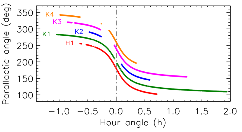
Figure 1: Parallactic angle coverage of the five observing runs. The numbering of the vertical axis is accurate for epoch H1; all other epochs have been translated upwards for visibility.

3 Data reduction

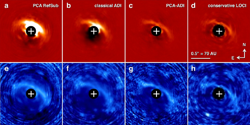
Figure 2: Comparison of four high-contrast data reduction methods applied to the K3 dataset of LkCa 15. The top row (a–d) shows the resulting images at a fixed linear stretch of $\pm 1.6\times 10^{-3}$ times the stellar peak flux. In order of decreasing conservation of disk flux: (a) PCA-assisted reference PSF subtraction, (b) classical ADI, (c) PCA-ADI, (d) conservative LOCI. The bottom row (e–h) shows the same images after renormalizing each concentric annulus around the star by the standard deviation of the pixel values in the annulus, at a stretch of $\pm 4\,\sigma$. The resulting images resemble signal-to-noise (S/N) maps, though the effective noise level is dominated by disk flux and thus overestimated in the inner $\sim$0$\aas@@fstack{\prime\prime}$5. Nevertheless, these images serve to reduce the dynamic range of the high-contrast images and visualize the characteristic crescent of positive disk flux left behind by the differential imaging methods.

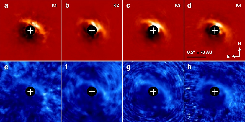
Figure 3: Comparison of the four Gemini NIRI $K_{\mathrm{s}}$-band observing runs of LkCa 15. All datasets were reduced with classical ADI. As in Figure 2, the upper row shows the resulting images at a linear stretch of $\pm 1.6\times 10^{-3}$ times the stellar peak flux, whereas the bottom row shows radially renormalized versions of the same images at a stretch of $\pm 4\,\sigma$. (a) K1, (b) K2, (c) K3, (d) K4. Since the target star is saturated in runs K1 and K2, their flux normalization is approximate.

Despite the efforts of the adaptive optics system, the faint scattered light from the LkCa 15 transitional disk is still overwhelmed by the diffraction halo of its host stars in all datasets. Differential imaging methods must be employed to remove as much of the star’s light as possible and recover the disk flux. Some of the disk flux is irretrievably lost in the process as well, rendering the reconstruction of the disk’s true appearance from the resulting images non-trivial (Thalmann et al., 2011; Milli et al., 2012; Thalmann et al., 2013). As discussed in Thalmann et al. (2013), the most rigorous way to infer physical disk properties from such data is to generate a parametric grid of plausible numerical disk models, calculate scattered-light images from those models, and subject the theoretical disk models to the exact same data reduction process as the science data. The resulting differential images can then be compared to those derived from the science data to constrain the range of disk parameters consistent with observations.

A number of differential imaging techniques are available for use with ADI data of circumstellar disks, offering a trade-off between effective suppression of the stellar halo (‘aggressive’ techniques) and conservation of disk flux (‘conservative’ techniques). The optimal choice of technique depends on the disk geometry, the circumstances of the observation, and the disk properties to be measured.

For the data at hand, we consider four differential imaging techniques, which we tested on the K3 dataset. The resulting images are presented in Figure 2. In order of increasing aggressiveness, the methods are:

PSF reference subtraction

based on principle component analysis (PCA; Soummer et al., 2012; Amara & Quanz, 2012). First, we used the Karhunen-Loève algorithm to decompose the dataset of the PSF reference star into a mean PSF plus an orthonormal base of principal component images. The image area within a radius of 6 pixels (0$\aas@@fstack{\prime\prime}$12) was masked out to prevent the star’s PSF core to dominate the definition of the principal components, as recommended in Amara & Quanz (2012). For each frame in the science dataset, we then subtracted the mean reference PSF and matched the first $n$ principal component templates to the science frame by least absolute deviation fitting, and subtracted them out. The science frames were then derotated and co-added to produce the final image. We selected $n=2$ on the basis of visual inspection of the results for $n=1\ldots 9$.

Classical ADI

as presented in Marois et al. (2006). An estimate of the stellar PSF is built by taking the mean of all science frames. The PSF is subtracted from all science frames, which are then derotated and co-added. We use mean-based frame collapse rather than median in order to improve the residual noise characteristics, as recommended in Brandt et al. (2013)

PCA-ADI

as employed by the PynPoint pipeline in Amara & Quanz (2012). This technique is essentially identical to the PCA-based PSF reference subtraction method described above, except that the science dataset itself is used as the basis for the principal component templates rather than an external PSF reference star. Again, we selected $n=2$ principal components to be subtracted.

Conservative LOCI

as introduced in Paper I and Buenzli et al. (2010). The LOCI algorithm (Locally Optimized Combination of Images; Lafrenière et al. 2007) is widely used in conjunction with ADI for direct imaging of planets and brown-dwarf companions (e.g., Marois et al., 2008; Thalmann et al., 2009; Lagrange et al., 2010; Carson et al., 2013). In its most common form, it is too aggressive to image astrophysical sources beyond the size of an isolated point source effectively; however, by choosing a stricter frame selection criterion (Paper I) or a larger optimization region area (Buenzli et al., 2010), the flux loss can be reduced far enough to make the method viable for the imaging of circumstellar disks. We refer to this use of LOCI as “conservative LOCI.” For our $K_{\mathrm{s}}$-band data, we find LOCI to be more aggressive than for the $H$-band data presented in Paper I—possibly due to the coarser plate scale—and therefore choose highly conservative LOCI parameters: a frame selection criterion of $N_{\delta}=5$ FWHM and an optimization area of $N_{A}=10,000$ PSF footprints. See Lafrenière et al. 2007 for detailed description of these parameters.

All data were flatfield-corrected and registered using Gaussian centroiding of the target star prior to the application of differential imaging. Since all datasets are either unsaturated or mildly saturated, the expected registration accuracy is $\leq$0.2 pixel (4 mas).

The dynamic range of the resulting images and the varying amounts of flux loss among the four reduction methods render the images difficult to compare directly. For this purpose, we renormalize the images by dividing the pixel values in each concentric annulus around the star by the standard deviation of those values. The resulting images resemble S/N maps, though the ‘noise’ level is dominated by the disk signal, and thus overestimated, out to $\sim$$0\aas@@fstack{\prime\prime}6$ (Figure 2e–h). Nevertheless, they serve to illustrate the signal content of the differential images qualitatively.

The images from all four data reduction methods paint a consistent picture of a crescent-shaped source of positive flux visually consistent in shape, size, and orientation with the $H$-band image published in Paper I, confirming that we are indeed detecting scattered light from the surface of the LkCa 15 pre-transitional disk. Perhaps surprisingly, the signal-to-noise map derived from PSF reference subtraction (Figure 2e) does not differ fundamentally from those made with ADI techniques (Figure 2f–h). Although the reference subtraction method avoids self-subtraction of the disk, the net positive disk flux still causes the template-fitting routine to overestimate and thus oversubtract the stellar halo in the science data. Therefore, none of these images yield an unbiased view of the LkCa 15 disk, making forward-modeling a necessity for quantitative analysis.

On the basis of Figure 2, we adopt classical ADI as our differential imaging method of choice for the rest of this work. Due to the saturation in epochs K1 and K2, PSF reference subtraction is ruled out. Of the remaining methods, classical ADI conserves the most disk flux, is numerically transparent and linear, and requires the least computation time. The latter point is relevant because the accuracy of a forward-modeling analysis is limited by the sampling of the multi-dimensional model parameter space, and thus by the number of models that can be evaluated in a reasonable timeframe.

Figure 3 shows the results of classical ADI applied to all four four $K_{\mathrm{s}}$-band datasets. Overall, the crescent of scattered light from the LkCa 15 transitional disk is consistently reproduced among the epochs. In particular, the position and orientation of the edge between the disk gap and the bright side of the illuminated disk surface can be measured reliably. The ansae of the disk gap are difficult to identify due to oversubtraction and low S/N ratios, though, and the faint side of the disk surface is not visible.

4 Modeling

4.1 Experiment design

Since the loss of disk flux in ADI image processing is irreversible, the only robust method of extracting astrophysical information on the LkCa 15 transitional disk from the data is forward modeling. This means generating a large number of plausible disk models by means of a radiative transfer code, simulating the observable appearance of those disks in scattered-light imaging using a raytracing code, and finally subjecting those images to the same ADI image processing that was applied to the science data. The family of disk models that yield ADI images consistent with those resulting from the science data can then be used to derive the best-estimate values and confidence intervals for the physical parameters of the disk.

Our forward-modeling setup comprises a total of nine independent free parameters:

• $r$, the radius of the disk’s transitional gap outer edge, or ‘wall’, represented by the scale factor $f:=(56\,\mathrm{AU})/r$,

• $i$, the inclination of its orbital plane,

• $g$, the Henyey-Greenstein forward-scattering efficiency of its dust grains,

• $w$, the ‘roundness’ of the gap wall,

• $s$, the vertical scale height of the inner disk, with $s=1$ corresponding to the canonical value derived from the SED (see Section 4.2),

• $o$, the orientation of the projected disk’s rotation axis (measured from North to East),

• $c$, the flux contrast between the disk and the star,

• ($x,y$), the offsets of the disk’s center from the star parallel and perpendicular to the line of nodes, respectively. The line of nodes is the intersection of the inclined disk plane with the “sky plane” perpendicular to the line of sight; it defines the unforeshortened “major axis” of the projected disk. The parameter $y$ includes foreshortening, its observed value is $\cos(i)$ times the physical offset along the disk plane.

The radiative transfer code does not support eccentric disks. However, since we discovered structure indicative of eccentricity in the LkCa 15 disk in Paper I, it is scientifically interesting to test this hypothesis in the analysis at hand. We therefore approximate eccentric disks by calculating scattered-light images of azimuthally symmetric disks, translating them by a small offset $(x,y)$ with respect to the star, and rescaling the brightness to take into account the new center of illumination. This is done in the third stage of our analysis (ADI processing).

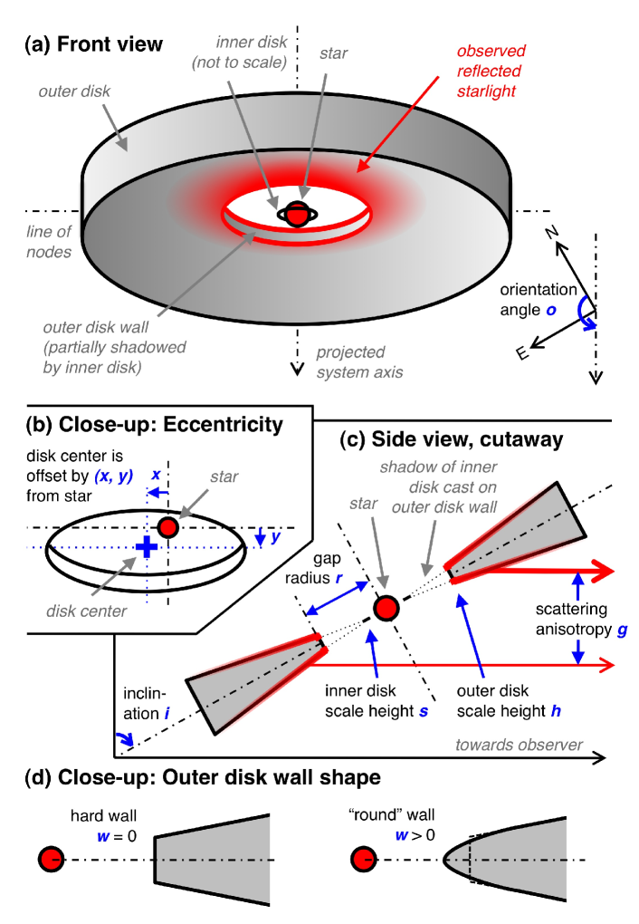
Figure 4: Sketch of the LkCa 15 system architecture as described by our model. Most of the bulk of the outer disk (shown in light grey) remains unseen; only the starlight reflected from its surface (shown in red) is observed with direct imaging. Anisotropic scattering behavior greatly enhances the forward-scattered flux on the disk’s near side, creating the bright crescent in the ADI images. The treatment of wall shape in our model is visualized in more detail in Figure 5. By default, the outer disk scale height $h$ is a fixed rather than a free parameter; see Section 5.9 and Appendix C.

Figure 4 provides a graphical visualization of the LkCa 15 system architecture as described by our model. Note that the sketches are not to scale – the SED predicts the inner truncation radius of the outer disk to be of order 50 AU, whereas the inner disk is contained at sub-AU radii. As a result, the inner disk is inaccessible to our direct imaging efforts, and can only impact our observations through the shadow it may cast on the wall of the outer disk.

The radiative transfer code used to generate self-consistent physical disk models is described in Section 4.2, the raytracing code employed to generate scattered-light images from the disk models in Section 4.3, and the ADI processing and $\chi^{2}$ evaluation in Section 4.4.

4.2 Radiative transfer code

The radiative transfer code used in this paper is MCMax (Min et al., 2009), a disk modeling tool that performs 3D dust radiative transfer in a 2D axisymmetric geometry. The code includes full anisotropic scattering and polarization (Min et al., 2012; Mulders et al., 2013a), making it an ideal tool for interpreting high-contrast images of protoplanetary disks.

Besides radiative transfer, it solves for the vertical structure of the disk using hydrostatic equilibrium and dust settling, yielding a self-consistent density and temperature structure. The dust scale height is in this case controlled by a scale factor $\Psi$, which represents the reduction in scale height of the dust compared to that of the gas.

The model employed here is based on the optically thick inner disk model described in Mulders et al. (2010, hereafter M10). The main modifications include:

Anisotropic scattering.

The M10 model did not include scattering in the radiative transfer step of the simulation.

Dust properties.

We changed the dust size and composition to roughly reflect the observed brightness asymmetry, such that the imaging constraints do not significantly alter the SED fit. The dust properties are described in the next section and shown in Table 2.

Round wall.

Steep gradients in surface density are not a natural outcome of planet-disk interactions (Lubow & D’Angelo, 2006; Crida & Morbidelli, 2007). Rather than a sudden increase at $r$, the surface density $\Sigma$ gradually increases with radius up to a radius $R_{\rm exp}$, after which it follows the surface density of the outer disk ($\Sigma_{\rm outer}\leavevmode\nobreak\ R^{-1}$). We use the exponential function described in Mulders et al. (2013b), which is characterized by a dimensionless width $w$ to described the spatial extent of this transition:

$$\Sigma(R<R_{\rm exp})\leavevmode\nobreak\ =\leavevmode\nobreak\ \Sigma_{\rm outer}\leavevmode\nobreak\ R^{-1}\leavevmode\nobreak\ \exp\left(-\left(\frac{1-R/R_{\rm exp}}{w}\right)^{3}\right).$$ (1)

This smoothly increasing surface density gives rises to a rounded-off wall in spatially resolved images, as shown in Figure 5. The wall extends further in than the anchor point for the exponential turnover ($R_{\rm exp}\sim[1...3]r$), depending on wall roundness). Instead, we use the radial peak in the intensity to trace the wall location $r$. Thus, $w$ represents the characteristic length scale of the exponential decay of the disk’s surface brightness at the gap edge. It is a dimensionless parameter normalized to the gap radius $r$. Both the wall location $r$ and its roundness $w$ are free parameters.

Stellar properties.

We use the updated stellar parameters from Andrews et al. (2011), listed in Table 2.

The dust contains two components with different size distributions ($a_{\rm small}$ and $a_{\rm big}$) and different degrees of settling ($s$ for the inner disk and $\Psi_{\rm small}$ and $\Psi_{\rm big}$ for the outer disk). $\Psi_{\rm small}$ and $\Psi_{\rm big}$ are constrained by fitting the mid-infrared SED. $s$ determines the size of the shadow cast on the outer disk wall. Although fitting the near-infrared excess yields $s\simeq 1$ (M10), we treat this parameter as free because the inner disk scale height is known to vary (Espaillat et al., 2011), and may be different for each observing epoch.

Since we updated both the stellar parameters and the dust composition since the M10, it was needed to refit all parameters to the observed SED (figure 6.). All fit parameters are shown in Table 2. Note that parameters $s$, $w$ and $g$ are also used in the radiative transfer step, but are free parameters.

Figure 5: Azimuthally averaged surface brightness profile (top) and corresponding surface density profile (bottom), demonstrating the effect of rounding off the disk wall ($w>0$). The solid line shows the best-fit model with a wall shape of $w=0.30$, compared to a more vertical wall with $w=0.05$ (dashed line). The dotted line indicates the “wall location” $r$, corresponding to the radial peak in intensity.

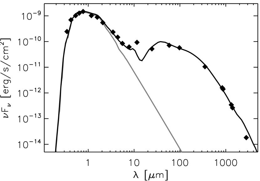
Figure 6: Spectral energy distribution of LkCa15. Displayed with the solid line is the best fit disk model described in table 2. References – (UBVRI) Kenyon & Hartmann (1995); (JHK) Skrutskie et al. (2006); Spitzer IRAC (Luhman et al., 2010); (IRAS) Weaver & Jones (1992); (submm) Andrews & Williams (2005); (mm) Piétu et al. (2006).

Model parameters Parameter Value $T_{\rm eff}\leavevmode\nobreak\ [{\rm K}]$ 4370 $L_{*}\leavevmode\nobreak\ [L_{\odot}]$ 1.22 $M_{*}\leavevmode\nobreak\ [M_{\odot}]$ 1.01 $d\leavevmode\nobreak\ [{\rm pc}]$ 140 $R_{\rm in}\leavevmode\nobreak\ [{\rm AU}]$ 0.07 $R_{\rm out}\leavevmode\nobreak\ [{\rm AU}]$ 300^† $R_{\rm gap}\leavevmode\nobreak\ [{\rm AU}]$ 4…56 $M_{\rm dust}\leavevmode\nobreak\ [M_{\odot}]$ 0.01 $M_{\rm dust,inner}\leavevmode\nobreak\ [M_{\odot}]$ $5\cdot 10^{-11}$ $p$ 1^† composition Solar^† $a_{\rm small}\leavevmode\nobreak\ [\mu{\rm m}]$ 0.1…1.5 $a_{\rm big}\leavevmode\nobreak\ [\mu{\rm m}]$ 100…500 $f_{\rm big,outer}\leavevmode\nobreak\ [\%]$ 99 $\Psi_{\rm small}$ 0.65 $\Psi_{\rm big}$ 0.2

Table 2: Disk parameters for the geometrical model. Fixed parameters are indicated by a dagger ($\dagger$). The surface density profile is defined as $\Sigma(r)\propto r^{-p}$ and scaled to the total disk mass. The location of the gap edge is approximate due to its smooth nature, displayed here is the peak of the radial intensity (Fig 5). Opacities are calculated assuming a grain size distribution $f(a)\propto a^{-3.5}$. Solar composition: 12% MgFeSiO₄, 12% MgFeSi₂O₆, 12% Mg₂SiO₄, 12% MgSi₂O₆, 15% FeS, 40% C. Optical constants are from: Silicates (Dorschner et al., 1995; Henning & Stognienko, 1996; Mutschke et al., 1998), Carbon (Preibisch et al., 1993), Troilite (Begemann et al., 1994).

4.2.1 Grain size

The absorption and scattering properties of the dust are set by the grain size, structure and composition (e.g., Van der Hulst, 1957). The main diagnostics of these properties in unpolarized images are the wavelength-dependent albedo (Fukagawa et al., 2010; Mulders et al., 2013a) and phase function (Duchene et al., 2004). Because the latter is a highly non-linear function of grain size, we use the Henyey-Greenstein phase function with assymetry parameter $g$ (Henyey & Greenstein, 1941) to prescribe the phase function of our particles, rather than varying the grain size. In doing so, we avoid having to refit the SED for each different grain size, as the grain properties can be kept fixed while varying $g$.

The grain composition is based on a condensation sequence for solar system elemental abundances as described in Min et al. (2011), see Table 2. We assume the grains have an irregular shape, parametrized by a distribution of hollow spheres (DHS) with a vacuum fraction ranging from 0 to 0.7 (Min et al., 2008). With an MRN size distribution (Mathis et al., 1977) from $0.1$ to $1.5$ micron, the albedo of these grains is $\sim$0.5 in $K$-band with a phase function close to $g=0.5$.

4.3 Scattered-light image simulation

The scattered light images are calculated by integrating the formal solution to the radiative transfer equations, using the density and temperature structure from the Monte Carlo simulation and the dust opacities as described above. The local scattered field is calculated in 3D using a Monte Carlo approach (see Min et al. 2012 for details). This scattered field includes a contribution both from the star and from the disk, which can be significant at near-infrared wavelengths.

First, the images are calculated for a given inclination angle $i$ in spherical coordinates, preserving the radial grid refinement at the gap outer edge. Finally, this image is mapped onto a cartesian grid matching the pixel scale of the observations, yielding a scattered light image that can be further processed by ADI. By employing a scale factor $f$ for the field of view, we generate multiple cartesian images with the same resolution but different field of view from the same spherical coordinates image. Hence, a larger field of view (large $f$) corresponds to a smaller gap. This greatly decreasing runtime of the entire grid by skipping the radiative transfer and raytracing step that would otherwise be associated with changing the gap radius $R$.

4.4 Forward-modeling of ADI observations

4.4.1 Theory

The raw science data $\mathcal{I}$ used as input for the ADI process can be described as a sum of the stellar PSFs $\mathcal{S}$ and the scattered-light images of the disk $\mathcal{D}$:

$$\mathcal{I}=\mathcal{S}+\mathcal{D}.$$ (2)

Since classical ADI using mean-based frame combination is linear (Marois et al., 2006), the resulting output image $\mathcal{O}$ produced by ADI processing of the imaging data $\mathcal{I}$ is equal to the sum of the ADI-processed stellar PSFs and the ADI-processed disk images:

$$\mathcal{O}=\mathrm{ADI}(\mathcal{I})=\mathrm{ADI}(\mathcal{S}+\mathcal{D})=\mathrm{ADI}(\mathcal{S})+\mathrm{ADI}(\mathcal{D}).$$ (3)

Since the stellar PSF remains largely static throughout the science data, ADI effectively removes the bulk of the stellar flux, leaving behind a halo of residual speckle noise. Given good adaptive optics performance (stable Strehl ratio) and enough field rotation (ideally across several resolution elements at all considered radii), the noise is well-behaved and approximately Gaussian in concentric annuli around the star.

$$\mathcal{O}=\mathrm{ADI}(\mathcal{D})+\mathrm{noise}.$$ (4)

Thus, applying the ADI process to a noise-free model disk image $\mathcal{D}_{\mathrm{mod}}$ yields an output image ADI($\mathcal{D}_{\mathrm{mod}}$) that can be directly compared with the resulting image from the science data. In the ideal case, subtracting the ADI-processed model image from the science data should leave behind only pure noise:

$$\mathcal{O}-\mathrm{ADI}(\mathcal{D}_{\mathrm{mod}}) = \mathrm{ADI}(\mathcal{D})+\mathrm{noise}-\mathrm{ADI}(\mathcal{D}_{\mathrm{mod}})$$ (5)

$$= [\mathrm{ADI}(\mathcal{D})-\mathrm{ADI}(\mathcal{D}_{\mathrm{mod}})]+\mathrm{noise}$$

$$\overset{!}{=} \mathrm{noise}.$$

Finally, assuming that the noise behaves in a Gaussian manner, one can define a $\chi^{2}$ metric to measure the goodness of fit for a given disk model:

$$\chi^{2}_{\mathrm{mod}}=\sum\frac{[\mathcal{O}-\mathrm{ADI}(\mathcal{D}_{\mathrm{mod}})]^{2}}{\sigma^{2}},$$ (6)

where $\sigma$ is a map of the local standard deviation of the noise.

4.4.2 Noise estimation

For highly inclined and well-resolved circumstellar disks, the radial noise profile can be measured in sectors of the final science image unaffected by the disk flux (e.g., Thalmann et al., 2011, 2013). However, the crescent of scattered light from the LkCa 15 disk, as well as the surrounding oversubtraction regions, dominate our ADI images at all position angles, rendering it impossible to measure an unbiased noise profile. During the exploratory phase of our experiment, we therefore started out with an estimated noise profile. As soon as we had located well-fitting models for each epoch, we iteratively redefined the noise profile for each dataset as the standard deviation of the pixel values in concentric annuli measured in the residual image $\mathcal{O}-\mathrm{ADI}(\mathcal{D}_{\mathrm{best}})$ for the best-fitting model disk $\mathcal{D}_{\mathrm{best}}$. Such an a posteriori definition of the noise profile yields a reduced $\chi^{2}$ of $\sim$1 for the best-fit model by design, and therefore cannot be used as an unbiased measure of absolute goodness of fit. However, it provides a useful measure of relative goodness of fit, allowing us to converge on a best-fit set of model parameters and to define confidence intervals around those parameters through a $\chi^{2}$ threshold.

The noise profiles obtained with this method furthermore are used to generate more meaningful S/N maps than the ones shown in Figures 2 and 3, since the disk flux no longer dominates the definition of the noise profile. The S/N map of the residual image, $[\mathcal{O}-\mathrm{ADI}(\mathcal{D}_{\mathrm{best}})]/\sigma$, provides a useful visual representation of the absolute goodness of fit, as well as a “sanity check” on the assumed a posteriori noise map. Ideally, it should look like random noise, with no coherent structure from the disk left behind. Similarly, the S/N map of the unsubtracted science ADI image, $\mathcal{O}/\sigma$, provides a measure of the significance of the retrieved disk signal, and thus of the scientific information content of the dataset.

4.4.3 Implementation

We perform the forward-modeling of ADI observations for our model disk images with a custom IDL code, which comprises the following steps:

• Load a simulated scattered-light disk model for a given set of parameters $(r,i,g,w,s)$.

• If $(x,y)$ are not zero, adjust the brightness distribution of the image to represent illumination by the off-centered star. For this purpose, we multiply each pixel by the square of its distance from the image center, then divide by the square of the distance from the new, offset position of the star. When calculating distances, we assume that all disk flux originates in the midplane; i.e., the projection effect from the plane’s inclination is taken into account, but not the finite scale height of the scattering disk surface.

• For each exposure $n$ in the science data, generate a corresponding ‘exposure’ of the model disk image. The position angle of the model disk in each frame is the input parameter $o$ plus the parallactic angle of the corresponding science exposure. As part of the image rotation, the intended position of the star $(x,y)$ in the model image is mapped onto the center of the model exposure. This way, the model images need only be resampled once, minimizing aliasing effects.

• Convolve each model exposure with a 15$\times$15 pixel image ($\approx$ 5 $\times$ 5 resolution elements) of the unsaturated PSF core of the corresponding science exposure. This lends the simulated disk data the appropriate spatial resolution while avoiding contamination of the model disk with the physical disk structure present in the science exposure at larger separations. In the case of saturated science data (epochs K1, K2), we substitute a single external PSF for all exposures.

• Perform classical ADI on the set of model exposures, yielding a noise-free ADI output image for the model disk.

• Bin down both the model output image and the science output image by a factor of 3 in both dimensions for the purpose of $\chi^{2}$ evaluation. Since the diffraction-limited resolution $\lambda/D$ is 57 mas = 2.8 pixels, neighboring pixels are always strongly correlated. After the binning, each pixel in the binned image can be treated as an independent data point. In practice, however, pixels may still be correlated to a certain degree due to large-scale structures remaining in the residual image. We retain the unbinned images for visualization purposes.

• Match the model output image to the science output image with a least-squares optimization of the model output image’s intensity scale factor. We make use of the linfit function in IDL, weighted with the a posteriori noise map $\sigma$. This defines the final free parameter of the disk model, the disk/star brightness contrast $c$.

• We subtract the model output image from the science output image and calculate the $\chi^{2}$ value of the residual image as per Equation 6, using the a posteriori noise map $\sigma$. We restrict the evaluation region to the annulus between the radii 0$\aas@@fstack{\prime\prime}$2 and 0$\aas@@fstack{\prime\prime}$8, thus excluding the center dominated by the stellar PSF core. The evaluation region comprises $N=516$ binned pixels, each of which roughly corresponds to a resolution element.

4.4.4 Confidence intervals

The best-fit disk model is defined as the set of input parameters yielding the minimum $\chi^{2}$ value, for each epoch of observation. We determine confidence intervals around those parameters by characterizing the family of ‘well-fitting’ solutions bounded by a threshold of $\chi^{2}\leq\chi^{2}_{\mathrm{min}}+\Delta\chi^{2}$. As in the case of our analysis of the HIP 79977 debris disk (Thalmann et al., 2013), we find that the pixels in our residual images do not have fully independent normal errors, as evidenced by traces of large-scale structure that remain visible in the S/N maps. Applying the canonical $\chi^{2}$ thresholds would not take into account those remaining systematic errors and thus overestimate the confidence in the best-fit parameters. We therefore choose a more conservative threshold of $\Delta\chi^{2}=32\approx\!\sqrt{2N}$, which corresponds to a $1\,\sigma$ deviation of the $\chi^{2}$ distribution with $N=516$ degrees of freedom. In other words, this threshold delimits the family of solutions whose residual images are consistent with the a posteriori noise map derived from the best-fit residual at the $1\,\sigma$ level.

Under the assumption that the disk image does not change significantly with time, a global best-fit solution and well-fitting solution family can be obtained by co-adding the four $\chi^{2}$ maps and adjusting the threshold $\Delta\chi^{2}$ by a factor of $\sqrt{4}=2$. The assumption is justified for most model parameters, since the disk gap is known to lie at a separation of $\sim$50 AU (Espaillat et al., 2008; Andrews et al., 2011), which implies an orbital time scale of several hundred years. Thus, we do not expect large-scale disk properties like the inclination, gap radius, or eccentricity of the outer disk to evolve measurably between our observing epochs. On the other hand, the inner component of the LkCa 15 pre-transitional disk orbits at sub-AU separations and may therefore evolve at a time scale of months. The model parameter $s$, which describes the vertical scale height of the inner disk and thus the width of the shadow band on the outer disk wall, must therefore be considered variable between K1, K2, and the pair of almost contemporary epochs (K3, K4). In any case, we present our results both for individual epochs and for the combined analysis in order to allow direct comparison. As reported in Section 5, no significant temporal variation is observed in any of the model parameters, including the inner disk scale height $s$. This validates the use of the global best-fit solution derived from all four epochs.

5 Results

5.1 Overview

In the early stages of this analysis, we explored parameter grids involving 2 or 3 model parameters at a time, keeping the other parameters fixed, and iterated this process until a stable $\chi^{2}$ minimum was located for each observing epoch. These preliminary best-fit (PBF) solutions are listed in Appendix A. While these models yielded visually convincing residuals and provided a necessary starting point for further analyses, they lacked confidence intervals and were not proven to be the global minima of the $\chi^{2}$ landscape. We do not document the specifics of these early searches in this work, since they are rendered obsolete by the further analyses presented in the following sections.

The most robust way to establish confidence intervals is a comprehensive, finely-sampled exploration of the 9-dimensional model parameter space. However, the radiative transfer simulation and the raytracing are computation-intensive procedures, which renders such a brute-force approach impracticable. We therefore seek to reduce the dimensionality of the parameter space as much as possible beforehand.

Simply exploring each parameter individually in one-dimensional analyses around the best-fit solution is not a valid approach, since some parameters are strongly covariant with each other. For instance, the most striking feature of the ADI images of LkCa 15 is the sharp transition from the dark disk gap to the brightest edge of the reflected light on the near side. For any given value of the gap radius $r$, there is only a narrow range of inclinations $i$ that project the gap edge onto the correct apparent separation from the star to match the data. However, a good match can be achieved over a much wider range of inclinations if the radius is adjusted proportionally. The well-fitting solution family therefore lies along a diagonal in the $(r,i)$ plane, and is ill-described by its cross-sections with the $r$ and $i$ axes.

Nevertheless, we find that 3 parameters can be safely decoupled from the full parameter space, and that one additional parameter requires only minimal sampling. This leaves only a manageable 5-dimensional parameter space to be explored thoroughly by brute-force calculations.

• $c$: The flux scaling of the model disk is set by least-squares optimization using the linfit function of IDL as part of the evaluation code (cf. Section 4.4.3). Thus, the disk/star contrast $c$ does not contribute a dimension to the parameter grid to be sampled.

• $x,o$: The gap center offset $x$ along the line of nodes (the “major” axis of the projected gap ellipse) and the orientation angle $o$ are the only two parameters whose effects on the disk image are not laterally symmetric. Thus, we expect them to have well-defined optima largely independent of the other model parameters.

• $s$: Our preliminary analyses surprisingly indicated that the achievable $\chi^{2}$ monotonously decreases with decreasing inner disk dust scale height $s$, reaching its minimum at $s=0$. $s=1$ corresponds to the hydrostatic equilibrium value of the inner disk scale height, which is supported by observations (Espaillat et al., 2008, 2010). Fractional values of $s\ll 1$ correspond to a razor-thin disk, which is not physically plausible. The special case of $s=0$, on the other hand, matches another physically plausible scenario: Either the inner disk is inclined with respect to the outer disk, such that most of the inner disk’s shadow bypasses the outer disk, or the inner disk is radially optically thin as described in M10, in both cases leaving the outer disk fully illuminated. We therefore limit the sampling in our analysis to the discrete values $s=\{0,0.5,1\}$ to verify this result.

5.2 Constraints on the orientation angle $o$ and on the center offset along the line of nodes $x$

In order to determine the best-fit values and confidence intervals for $x$ and $o$, we run three-dimensional parameter grids varying $(x,o,r)$ and keeping all other parameters fixed at their preliminary best-fit values. The disk radius $r$ is included a grid parameter in order to allow the positions of the two ansae along the line of nodes ($\pm r+x$) to be optimized independently of each other.

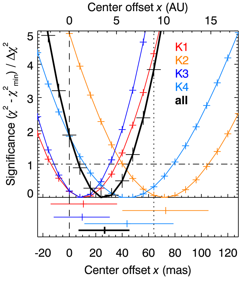
Figure 7: Constraints on disk center offset $x$ along the line of nodes. The plot shows the excess of the best-fit $\chi^{2}$ for a given $x$ with respect to the minimal $\chi^{2}_{\mathrm{min}}$ achieved, normalized by the threshold value $\Delta\chi^{2}$. The color-coded curves represent each individual epoch, whereas the thick black curve is obtained by combining all four epochs. The dashed line marks the case of a laterally symmetric disk ($x=0$), whereas the dotted line marks the tentative offset postulated in Paper I. Positive values of $x$ represent offsets in the direction of the western ansa.

The bottom panel shows the well-fitting range and the best-fit value for all five analyses.

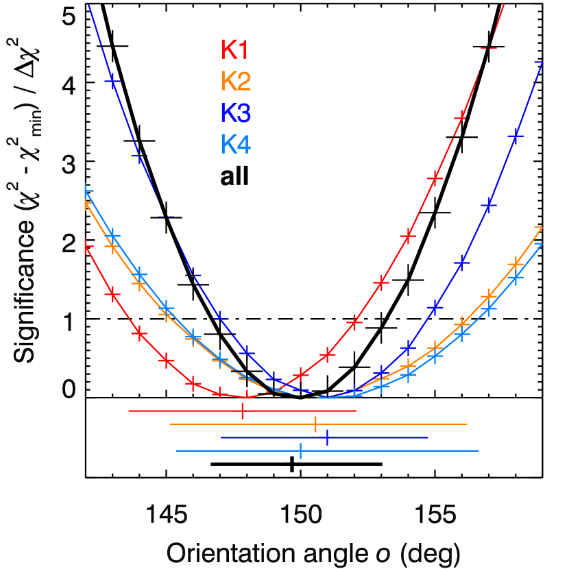
Figure 8: Constraints on the orientation angle $o$ of the disk’s rotation axis. The plot shows the excess of the best-fit $\chi^{2}$ for a given $o$ with respect to the minimal $\chi^{2}_{\mathrm{min}}$ achieved, normalized by the threshold value $\Delta\chi^{2}$. The color-coded curves represent each individual epoch, whereas the thick black curve is obtained by combining all four epochs. The angle $o$ is measured counter-clockwise from North to East. The bottom panel shows the well-fitting range and the best-fit value for all five analyses.

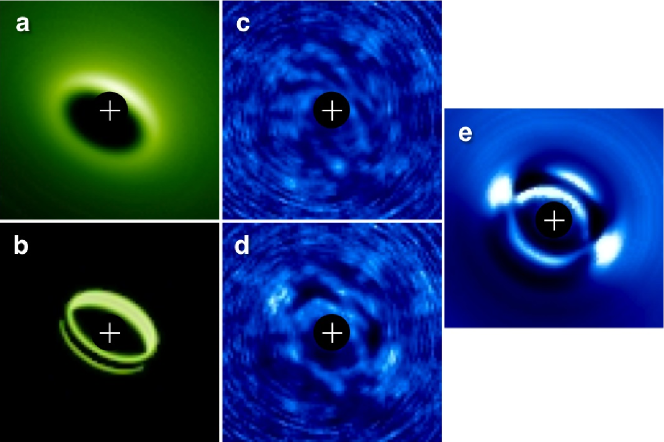
Figure 9: Comparison of the best-fit solutions for the near-side scenario ($g=0.7$, $o=150^{\circ}$) and the far-side scenario ($g=0$, $o=230^{\circ}$) for the K3 dataset. (a) Image of the unconvolved best-fit model near-side disk model, at logarithmic stretch. (b) The same for the best-fit far-side model. Note that in this configuration, the dark lane on the faint side is not generated by the shadow cast from the inner disk, but rather by the optically thick bulk of the outer disk blocking the view onto the illuminated face of the gap wall. The two parallel arcs of light are scattered light spilling around the edges of the near-side wall. (c) S/N map of the residual image after subtracting the ADI-processed near-side model image from the ADI-processed data, at a linear stretch of $\pm 5\,\sigma$. (d). The same for the far-side model. (e). Difference of the images (d) $-$ (c), at a linear stretch of $\pm 2\,\sigma$. The $\chi^{2}$ of the far-side model exceeds that of the near-side model by 18 $\Delta\chi^{2}$. We therefore conclude that the bright crescent in the data represents the strongly forward-scattering near side of the disk.

Figures 7 and 8 show the resulting best-fit values and domains of the well-fitting solution families for $x$ and $o$, respectively. The families from the four epochs appear as well-behaved $\chi^{2}$ curves with unique minima. While the $o$ values from different epochs agree well, the $x$ values exhibit some scatter, in particular in the lower-quality epochs K2 and K4.

We find that the best-fit offsets $x$ consistently lie on the positive (western) side of the star in all four epoch, though the offsets for the two high-quality datasets K1 and K3 are consistent with zero. Adding up the four $\chi^{2}$ maps yields global best-fit values and well-fitting intervals of $x=+24$ $[+7,+45]$ mas (corresponding to $+3$ $[+1,+6]$ AU in physical distance) and $o=150$ $[147,153]$ degrees. A summary of all numerical results from this analysis is included in Table 3.

In Paper I, we postulated a tentative disk center offset of $x=+64$ mas with a phenomenological error bar of $\pm 6$ mas on the basis of the H1 dataset. This error did not take into account the bias and systematic uncertainties from the ADI reduction, and therefore overestimated the accuracy of the measurement. However, the measured value is consistent with those of our lower-quality datasets K2 and K4, whose S/N maps exhibit a similarly ‘patchy’ structure as that of H1. The spread in $x$ values may therefore be due to a bias caused by marginal lateral constraints on the gap; i.e., the optimization of $x$ might be dominated by large-scale residual noise rather than by the actual disk flux in the lower-quality datasets. The fact that all five measurements of $x$ have the same sign suggests an underlying physical asymmetry that may be exaggerated by ADI under low S/N conditions.

Thus, overall, our analysis tentatively confirms the existence of a positive disk center offset in $x$ direction, though at a significantly smaller magnitude than proposed in Paper I.

Note that for all our best-fit models, the bright crescent apparent in the ADI images is generated by the near side of the disk, where the scattered light is greatly enhanced by anisotropic forward scattering (‘near-side scenario’). This is in agreement with the predictions of Piétu et al. (2007) based on asymmetries in their millimeter interferometry images. Furthermore, our orientation angle agrees very well with their value of $o=150.7^{\circ}\pm 0.4^{\circ}$.

In (Paper I), we demonstrated that it is possible to make the far side of the disk rim brighter than the near side within the parameter space of our model, allowing for the ‘far-side scenario’ as an alternative explanation for the bright crescent in the ADI data. In this scenario, the scattering anisotropy is minimal ($g\approx 0$), and the contrast is instead generated by self-shadowing of the near-side gap wall, leaving only the illuminated far-side wall exposed to imaging. To explore this possibility, we have run a limited parameter grid of models with $o=230^{\circ}$, $g=0$, coarse sampling of $s$ and $w$, and fine sampling of $i$, $f$, and $y$. The latter three parameters are most likely to influence the near-to-far side contrast.

The results are shown in Figure 9. While the far-side scenario is capable of achieving a contrast comparable to the one in the near-side scenario, it requires the visible scattered light to be tightly constrained to the gap wall. The resulting image is a poor match for the observed radially extended disk morphology. The best $\chi^{2}$ attained with the far-side model exceeds that of the near-side model by 18 $\Delta\chi^{2}$. We therefore conclude that the bright crescent of scattered light in the LkCa 15 disk represents starlight forward-scattered off the near-side surface of the outer disk.

5.3 Brute-force optimization and best-fit solutions

Having obtained best-fit solutions for $x$ and $o$, we perform a brute-force exploration of the remaining parameter space, with fine sampling in $f,i,g,w,y$, discrete sampling in $s$, and least-squares fitting in $c$. Table 3 defines the range and step size of the sampling in all parameter dimensions.

We find well-defined $\chi^{2}$ minima for all four epochs. Table 3 lists the model parameters corresponding to these best-fit solutions, as well as the parameter ranges of the well-fitting solution family obtained with a threshold of $\chi^{2}+\Delta\chi^{2}$ as defined in Section 4.4.4. A better characterization of the well-fitting solution family and the covariances between the model parameters is provided by the $\chi^{2}$ contour plots in the following subsections.

Table 3: Best-fit values, 1 $\Delta\chi^{2}$ confidence ranges, and definition of the sampling grid for the LkCa 15 model parameters.

		K1		K2		K3		K4		all epochs
Parameter	Search grid	best	range	best	range	best	range	best	range	best	range
Radius $r=56\,\mathrm{AU}/f$	43.1…70.0	61.0	[53.1, 67.7]	54.8	[44.7, 67.5]	54.8	[49.5, 62.3]	56.2	[49.6, 63.0]	56.3	[52.0, 62.6]
Inclination $i$ (∘)	28, 30, …, 70	51	[46, 57]	54	[43, 62]	47	[43, 53]	44	[36, 52]	50	[44, 54]
Henyey-Greenstein $g$	0.45, 0.50, …, 0.90	0.60	[ 0.45, 0.76]	0.86	[0.67, 0.90]	0.72	[0.55, 0.90]	0.60	[ 0.45, 0.84]	0.67	[0.56, 0.85]
Wall shape $w$	0.05, 0.10, …, 0.40	0.30	[ 0.05, 0.38]	0.31	[ 0.05, 0.40]	0.27	[ 0.05, 0.36]	0.32	[0.17, 0.40]	0.31	[0.19, 0.36]
Inner disk settling $s$	0, 0.5, 1	0	$\ll 1$	0	$\ll 1$	0	$\ll 1$	0	$\ll 1$	0	$\ll 1$
Offset $x$ (mas)(1)	$-24$, $-16$, …, $+128$	$+11$	[$-14$, $+36$]	$+73$	[$+40$, $+105$]	$+10$	[$-12$, $+31$]	$+44$	[$+11$, $+79$]	$+27$	[$+7$, $+46$]
—, (AU)	$-3$, $-2$, …, $+18$	$+1$	[$-2$, $+5$]	$+10$	[$+6$, $+15$]	$+1$	[$-2$, $+4$]	$+6$	[$+2$, $+11$]	$+4$	[$+1$, $+6$]
Offset $y$ (mas)	$-140$, $-130$, …, 0	$-64$	[$-111$, $-27$]	$-64$	[ $-140$, $-6$]	$-84$	[$-131$, $-40$]	$-100$	[ $-140$,$-47$]	$-69$	[$-118$, $-44$]
—, deprojected (AU)	$-41$, $-39$, …, 0	$-14$	[$-24$, $-6$]	$-14$	[ $-30$, $-1$]	$-18$	[$-29$, $-9$]	$-22$	[ $-30$, $-10$]	$-15$	[$-26$, $-10$]
Orientation $o$ (∘)(1)	142, 143, …, 159	148	[144, 152]	151	[145, 156]	151	[147, 155]	150	[145, 157]	150	[147, 153]
Flux ratio $c$ (%)	least-squares fitting	3.1(2)	[2.8, 3.6]	2.9(2)	[2.5, 4.2]	2.6	[2.2, 2.9]	2.3	[1.7, 2.5]	—
Notes. — (1) The parameters $x$ and $o$ were not sampled as part of the brute-force grid calculation, but in a separate analysis beforehand. (2) Disk/star contrast measurements from epochs K1 and K2 are unreliable, since the target star is saturated in the science data. (3) Where the well-fitting ranges exceed the bounds of the sampled parameter grid, the grid bounds are listed (in gray color). Note that the range of the combination of all four epochs (last column) is fully enclosed in the grid.

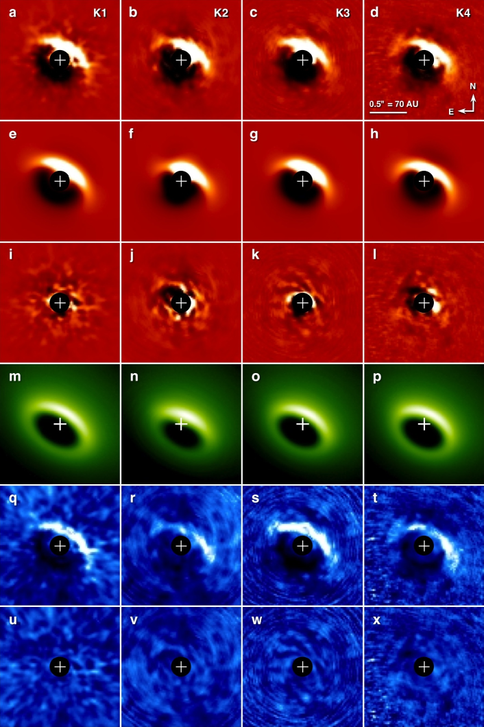
Figure 10: Best-fit models for the LkCa 15 disk. The columns represent the four epochs of observation, K1–K4. (a–d) ADI output images from science data; (e–h) ADI output images from the simulated model disks; (i–l) science–model subtraction residuals at the same linear stretch; (m–p) unprocessed model disk images at logarithmic stretch; (q–t) S/N maps of the science ADI output images at a linear stretch of $[-5\sigma,5\sigma]$; (u–x) S/N maps of the subtraction residuals at the same stretch.

Figure 10 presents a visual overview of the best-fit model solutions and their agreement with the data for each epoch of observation. The first row displays the classical ADI images derived from the data, while the second row shows the classical ADI images generated from the best-fit model disk images with the same set of parallactic angles. The third row represents the subtraction residuals of the first two rows, demonstrating that the overall morphology of the data is well explained by the models. The residuals are largely unstructured and well-behaved; only in K2 a coherent arc reminiscent of the disk structure is retained. There are no consistently recurrent features apparent in the four residual images that would suggest observable disk structure beyond the scope of the model parameter space, such as spirals, clumps, gaps, or planets.

The fourth row exhibits the unprocessed simulated scattered-light images of the best-fit model disks in logarithmic stretch. The disk architectures are roughly consistent between the epochs. Note that the position of the disk center is consistently offset from the star, bringing the bright near side of the disk rim closer to the star. In our model parametrization, this corresponds to a negative value of $y$. This observation is further discussed below in Section 5.9.

The fifth and sixth rows of Figure 10 show the S/N maps corresponding to the original ADI output images (first row) and subtraction residuals (third row), using the a posteriori radial noise map derived from the residuals (third row), as discussed in Section 4.4.2. This reduces the dynamic range of the images, allowing residual structures at various radii to be compared directly. The images of the fifth row furthermore offer an estimate of the overall information content of each observing run. Since the original disk flux can be assumed as approximately constant, the S/N at which the disk is detected at a given location is a measure of sensitivity and effectiveness of noise suppression.

We can obtain a numerical measure of the information content in each dataset by calculating the reduced $\chi^{2}$ of the raw ADI images, which is defined as the RMS of the S/N map divided by the number of pixels in the evaluation area. The resulting numbers are given in Table 4. This confirms our choice of K3 as the most reliable dataset, and explains the inferior performance of K2 in Figure 10.

Table 4: Information content of the four datasets, as measured by the reduced $\chi^{2}$ of the a posteriori S/N map of the raw ADI disk image. A higher reduced $\chi^{2}$ implies an ADI image that is more inconsistent with being pure noise, i.e., with more disk flux measurable above the noise threshold.

	K1	K2	K3	K4
Reduced $\chi^{2}$	3.9	2.1	5.4	2.5

5.4 Constraints on the wall shape parameter $w$

Figure 11 presents the minimum $\chi^{2}$ achieved in our brute-force grid search as a function of the gap wall shape parameter $w$. The best-fit solutions of all four epochs lie within the narrow interval of $w=[0.27,0.31]$. While two individual epochs cannot exclude the possibility of an abrupt ‘vertical’ wall ($w\approx 0$), the combined analysis yields a well-fitting range of $w=[0.19,0.36]$, clearly favoring an extended, ‘fuzzy’ radial transition from gap to outer disk.

Figure 12 illustrates the difference between a round wall $(s=0.30)$ and a vertical wall $(s=0.05)$ for the epoch K3. We find no significant codependence of the best-fit value of $w$ with other model parameters.

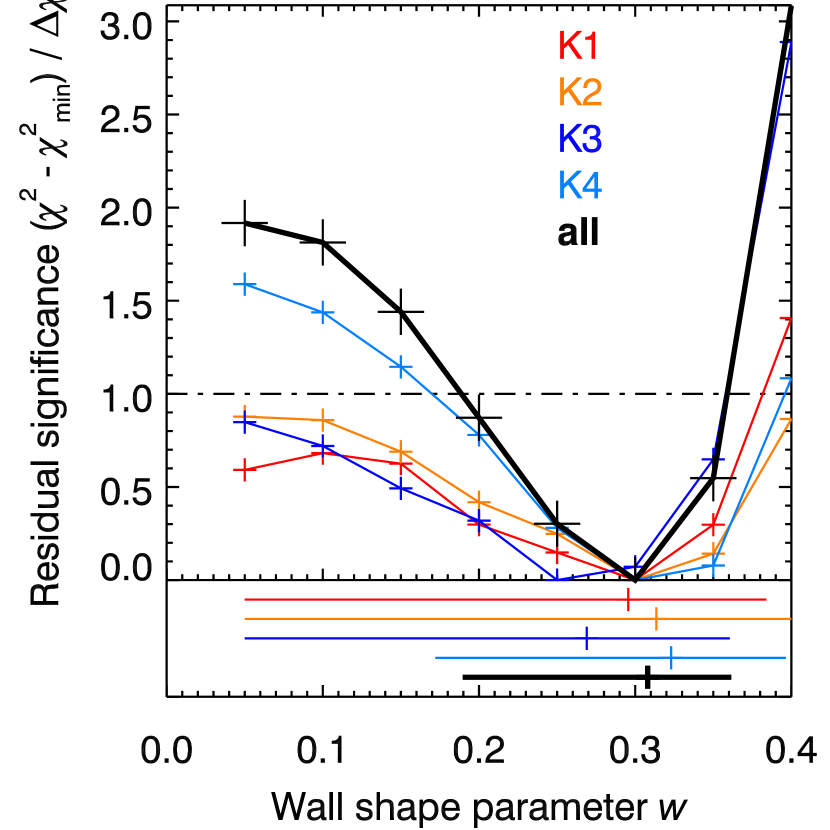
Figure 11: Constraints on the wall shape parameter $w$. The plot shows the excess of the best-fit $\chi^{2}$ for a given $w$ with respect to the minimal $\chi^{2}_{\mathrm{min}}$ achieved, normalized by the threshold value $\Delta\chi^{2}$. The color-coded curves represent each individual epoch, whereas the thick black curve is obtained by combining all four epochs. The bottom panel shows the well-fitting range and the best-fit value for all five analyses. The global best fit is achieved for $w=0.31$, suggesting that the gap wall of the outer disk is ‘fuzzy’, extending over a significant range of radii rather than being sharply constrained to a given radius ($w\approx 0$). The bottom panel shows the well-fitting range and the best-fit value for all five analyses.

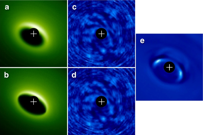
Figure 12: Comparison of the best-fit solutions for $w=0.30$ and $w=0.05$ for the K3 dataset. (a) Image of the unconvolved best-fit model disk with $w=0.30$, at logarithmic stretch. (b) The same for $w=0.05$. (c) S/N map of the residual image after subtracting the ADI-processed best-fit model image with $w=0.30$ from the ADI-processed data, at a linear stretch of $\pm 5\,\sigma$. (d). The same for $w=0.05$. (e). Difference of the images (d) $-$ (c), at a linear stretch of $\pm 2\,\sigma$. The $\chi^{2}$ of the $w=0.05$ model exceeds that of the $w=0.30$ model by 0.85 $\Delta\chi^{2}$.

5.5 Constraints on inner disk settling $s$

Figure 13: Constraints on the inner disk vertical settling parameter $s$. The plot shows the excess of the best-fit $\chi^{2}$ for a given $s$ with respect to the minimal $\chi^{2}_{\mathrm{min}}$ achieved, normalized by the threshold value $\Delta\chi^{2}$. The color-coded curves represent each individual epoch, whereas the thick black curve is obtained by combining all four epochs. In all cases, the best fit is achieved with $s=0$, i.e., with a completely absent inner disk shadow.

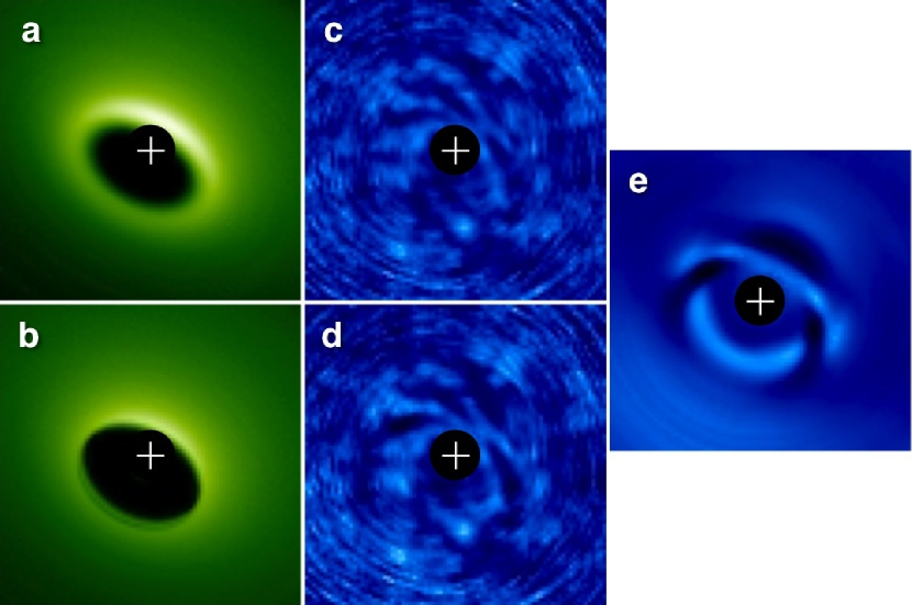
Figure 14: Comparison of the best-fit solutions for $s=0$ and $s=1$ for the K3 dataset. (a) Image of the unconvolved best-fit model disk with $s=0$, at logarithmic stretch. (b) The same for $s=1$. Note the lane of shadowing from the inner disk visible on the far-side gap wall. (c) S/N map of the residual image after subtracting the ADI-processed best-fit model image with $s=0$ from the ADI-processed data, at a linear stretch of $\pm 5\,\sigma$. (d). The same for $s=1$. (e). Difference of the images (d) $-$ (c), at a linear stretch of $\pm 2\,\sigma$. The $\chi^{2}$ of the $s=1$ model exceeds that of the $s=0$ model by 7.4 $\Delta\chi^{2}$.

Figure 13 shows a plot of the minimal $\chi^{2}$ achieved in our brute-force grid search for each of the three considered values of the inner disk settling parameter $s=\{0,0.5,1\}$, in comparison to the global $\chi^{2}$ minimum. As expected on the basis of our preliminary analyses (cf. Section 5.1), the global best fit is achieved with $s=0$ for all epochs, whereas the best fits attainable with $s=1$ exceed the global $\chi^{2}$ minimum by 3–7 $\Delta\chi^{2}$ ($10\,\Delta\chi^{2}$ for all four epochs combined).

The figure suggests that the criterion for a well-fitting solution ($\chi^{2}\leq\chi^{2}_{\mathrm{min}}+\Delta\chi^{2}$) is only achievable with $s\ll 1$. Taken at face value, this implies an unphysically small scale height for the inner disk, given that $s=1$ represents the expected hydrostatic equilibrium value that is compatible with the observed near-infared excess. However, an inner disk inclined with respect to the outer disk would leave most of the outer disk wall unshadowed, and thus provide a physical scenario for $s=0$. We note that the alternative scenario of an optically thin dust halo in place of the inner disk, as proposed in Espaillat et al. (2007) and investigated in Mulders et al. (2010), is also compatible with $s=0$, but the existence of such a halo is difficult to justify from a physical point of view (Espaillat et al. 2010, however, see Krijt & Dominik 2011).

Figure 14 illustrates the differences between the best-fit solutions for $s=0$ and $s=1$. The shadow of the inner disk on the outer disk wall is visible as a dark ribbon in the $s=1$ model image (Fig. 14b). The two illuminated edges of the wall are separated by slightly less than a resolution element, and therefore cannot be distinguished in our data. However, note that the effect of shadowing from the inner disk in the $s=1$ case is not restricted to the faint far-side gap wall, as one might expect. While the near-side wall would be self-shadowed in the case of a vertical cutoff ($w=0$), its upper half remains exposed to direct view in the case of a tapered disk edge ($w>0$), which is favored by our analysis (cf. Section 5.4). Thus, the inner disk shadow visibly truncates the inner edge of the tapered disk wall, hardening the gradient between the illuminated disk surface and the gap at all azimuths. As a result, our analysis is more sensitive to the degree of shadowing than the low S/N ratio of the far-side gap edge would suggest.

Unlike all other model parameters, $s$ pertains to the inner rather than the outer disk, which has an orbital time scale of months rather than decades. As a result, it is the only parameter for which one may expect astrophysical variation from one observing epoch to the next. However, we find consistent results for $s=0$ in all datasets.

We therefore conclude that, within the parameter space of our modeling effort, an inner disk inclined with respect to the outer disk is the most likely scenario for LkCa 15.

5.6 Constraints on the outer disk wall radius $r$

Figure 15 shows the $\chi^{2}$ plot for the outer disk wall radius $r$. The four epochs roughly agree with each other, with a global best-fit value of $r=56$ AU and well-fitting solutions for the span of $r=[52,63]$ AU. This measurement is in excellent agreement with the value of $r=58$ AU derived solely on the basis of the SED by Espaillat et al. (2010).

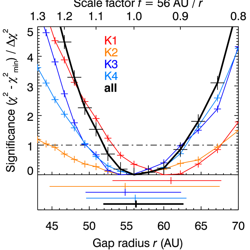
Figure 15: Constraints on the outer disk wall radius $r$, represented in our model by the scale factor $f=56\,\mathrm{AU}/r$. The plot shows the excess of the best-fit $\chi^{2}$ for a given $r$ with respect to the global minimum $\chi^{2}_{\mathrm{min}}$, normalized by the threshold value $\Delta\chi^{2}$. The color-coded curves represent each individual epoch, whereas the thick black curve is obtained by combining all four epochs. The bottom panel shows the well-fitting range and the best-fit value for all five analyses.

5.7 Constraints on the inclination $i$

Figure 16 presents the $\chi^{2}$ plot for the inclination $i$ of the disk plane. While there is some scatter among the lower-quality epochs, the combination of all four epochs yields a very well-behaved $\chi^{2}$ profile, with the best-fit solution at $i=50^{\circ}$ and well-fitting solutions spanning $i=[44^{\circ},54^{\circ}]$. This is in excellent agreement with the $i=51.5^{\circ}\pm 0.7^{\circ}$ inferred by Piétu et al. (2007) from molecular line emission and confirmed by Andrews et al. (2011), but notably higher than the $i=42^{\circ}$ assumed by Espaillat et al. (2010).

Figure 16: Constraints on the inclination $i$ of the disk plane. The plot shows the excess of the best-fit $\chi^{2}$ for a given $i$ with respect to the global minimum $\chi^{2}_{\mathrm{min}}$, normalized by the threshold value $\Delta\chi^{2}$. The color-coded curves represent each individual epoch, whereas the thick black curve is obtained by combining all four epochs. The bottom panel shows the well-fitting range and the best-fit value for all five analyses.

5.8 Constraints on the Henyey-Greenstein parameter $g$

Figure 17 displays the $\chi^{2}$ plot for the Henyey-Greenstein parameter $g$, which describes the degree of anisotropic forward-scattering. There is a considerable amount of diversity among the epochs, with local best-fits ranging from $g=0.60$ to $g=0.86$. Since $g$ is a property of the size and shape distribution of the dust grains in the outer disk, it is not expected to exhibit any real astrophysical variation. We therefore conclude that these variations represent measuring uncertainy, and that the exact value of $g$ is difficult to pinpoint with our analysis approach. Note that the Henyey-Greenstein formalism is a simplification of dust scattering behavior, and may thus be an inaccurate description of the dust phase function at hand. We do not consider values of $g>0.9$, since the Henyey-Greenstein formalism becomes very inaccurate in that regime.

Nevertheless, combining the $\chi^{2}$ curves of the four epochs yields a clear best-fit solution at $g=0.67$ and well-fitting solutions for the range of $g=[0.56,0.85]$. All of these values are notably on the high end of the range expected for circumstellar disks, which explains the extremely high contrast observed between the near and far sides of the disk in scattered light (see also Figure 21).

Because the system model is symmetric, one could argue that there is the possibility that the disk is oriented in the opposite way, i.e. the far side being the bright side, and the grains have a negative assymmetry parameter $g$. The phase function of aggregate particles can be backward scattering over a limited range of scattering angles (see e.g., Min et al., 2010). In our case, the scattering angles of the far side and the near side of the disk are approximately 134 and 34^∘ respectively (given that the opening angle of the disk at the location of the wall is approximately 6^∘ and the inclination is 50^∘). To get the same contrast between these two scattering angles with a negative value of $g$, one would need $g<-0.9$, which is highly unphysical.

Figure 17: Constraints on the Henyey-Greenstein parameter $g$. The plot shows the excess of the best-fit $\chi^{2}$ for a given $g$ with respect to the global minimum $\chi^{2}_{\mathrm{min}}$, normalized by the threshold value $\Delta\chi^{2}$. The color-coded curves represent each individual epoch, whereas the thick black curve is obtained by combining all four epochs. The bottom panel shows the well-fitting range and the best-fit value for all five analyses.

5.9 Constraints on the center offset perpendicular to the line of nodes $y$

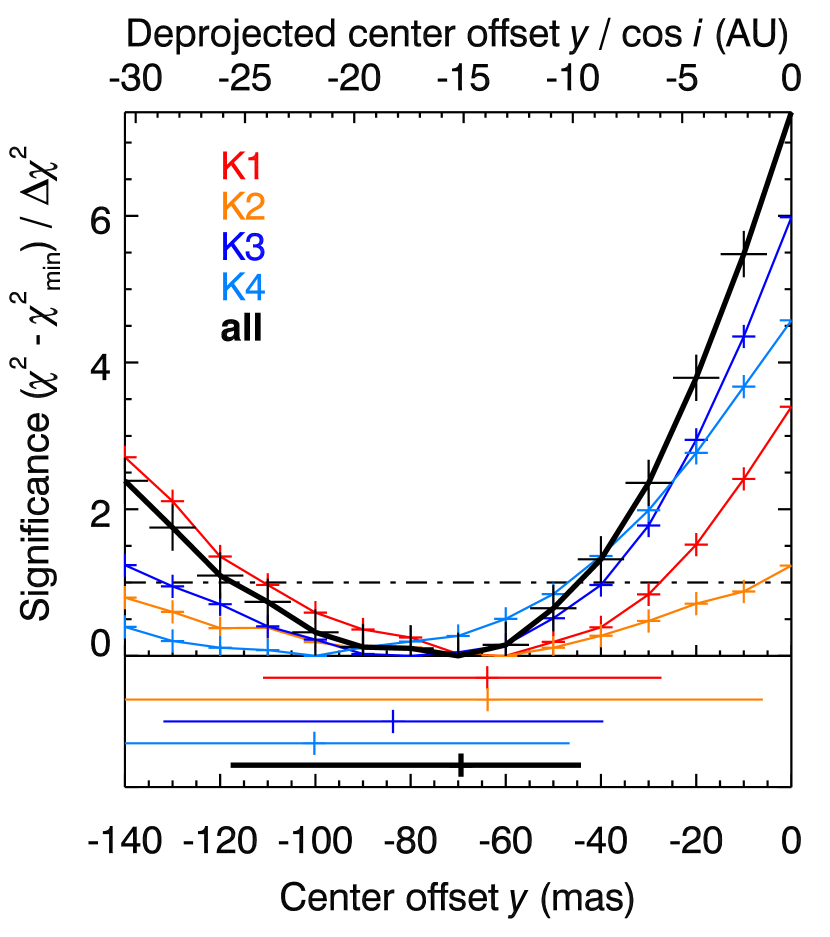
Figure 18: Constraints on the disk center offset $y$ perpendicular to the line of nodes. The plot shows the excess of the best-fit $\chi^{2}$ for a given $y$ with respect to the global minimum $\chi^{2}_{\mathrm{min}}$, normalized by the threshold value $\Delta\chi^{2}$. The color-coded curves represent each individual epoch, whereas the thick black curve is obtained by combining all four epochs. The bottom panel shows the well-fitting range and the best-fit value for all five analyses.

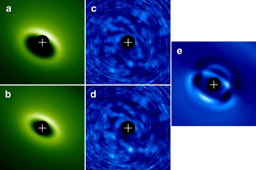
Figure 19: Comparison of the best-fit solutions for $y=-80$ mas and $y=0$ mas for the K3 dataset. (a) Image of the unconvolved best-fit model disk with $y=-80$ mas, at logarithmic stretch. (b) The same for $y=0$ mas. (c) S/N map of the residual image after subtracting the ADI-processed best-fit model image with $y=-80$ mas from the ADI-processed data, at a linear stretch of $\pm 5\,\sigma$. (d). The same for $y=0$ mas. (e). Difference of the images (d) $-$ (c), at a linear stretch of $\pm 2\,\sigma$. The $\chi^{2}$ of the $y=0$ mas model exceeds that of the $y=-80$ mas model by 6.0 $\Delta\chi^{2}$.

Figure 18 shows the $\chi^{2}$ plot for the offset $y$ of the disk center from the star position perpendicular to the line of nodes. The four epochs agree well with each other. Combining the $\chi^{2}$ curves from all epochs yields a best-fit solution of $y=-69$ mas, with well-fitting solutions for a range of $y=[-118,-44]$ mas. Accounting for the foreshortening due to the inclined disk, this implies a surprisingly large physical offset of $y=15\leavevmode\nobreak\ [10,26]$ AU along the disk plane. Given the gap radius of $r\approx 56$ AU, this configuration corresponds to an eccentricity of $e\approx 0.3$. Figure 19 illustrates the difference between the eccentric best-fit solution for the K3 data and the restricted best-fit solution with $y=0$ mas.

Since this study is the first to measure the disk center offset along this dimension, its discovery is to be treated with caution until it can be confirmed independently. As Figure 18 demonstrates, our combined $\chi^{2}$ analysis rejects the default hypothesis of $y=0$ at the $7.5\Delta\chi^{2}$ level, thus there is little doubt that a strong $y$ offset is necessary for a best-fit solution within our model grid. However, we acknowledge the possibility that this offset represents the model’s effort to match a feature of disk architecture beyond the scope of its parameter space.

One degree of freedom that can conceivably be responsible for an apparent shift of the disk image perpendicular to the line of nodes is the effective scale height of the outer disk, represented in our model by the internal parameter $\Psi_{\mathrm{small}}$. As it increases, the upper and lower surfaces of the disk move apart in the projected image. Since only the upper surface is seen in our reflected-light images, a change in $\Psi_{\mathrm{small}}$ may be perceived as a change in $y$ in our model.

The outer disk scale height is not treated as a free parameter of our model approach, since its default value $\Psi_{\rm small}=0.5$ is constrained by the far-infrared SED (Mulders et al., 2010). However, we ran a small-scale parameter analysis to determine whether its introduction as a free model parameter would remove the need for a $y$ offset. This analysis is described in Appendix C. In order to keep the nomenclature consistent with the other free model parameters, in particular with the inner disk scale height $s$, we named the new free model parameter $h:=2\,\Psi_{\rm small}$. This defines the default outer disk scale height as $h=1$, in analogy with the default inner disk scale height $s=1$.

In the small-scale parameter analysis, we explored the extreme case of $h=2$ ($\Psi_{\rm small}=1$; i.e., an inner disk scale height of twice the expected value). We found that the overall fit quality decreased significantly with respect to the default $h=1$ case, whereas the best-fit value of $y$ did not change significantly from its $h=1$ best-fit value. We therefore rejected the use of $h$ as a free parameter and kept $h=1$ fixed for our main analysis. A physical offset of the disk center from the star remains our best explanation for the observed disk images at this point.

We note that our model implements an eccentric disk as a circular disk shifted away from the star. For low eccentricities $e\ll 1$, this method approximates an elliptical gap well. At the observed eccentricity of $e=0.3$, though, the approximation is quite inaccurate. We therefore acknowledge that our best-fit model likely cannot represent the disk’s true shape in all aspects, and that more elaborate disk models including elliptical or even spiral-like disk architectures may yield improved fits in the future.

5.10 Covariances between $r,i,g,w,y$

In Section 5.1, we opted for a brute-force parameter grid search in the five model dimensions $r,i,g,w,y$, since we expected that covariances between these parameters might render an independent optimization of each individual parameter impractical. Having calculated the $\chi^{2}$ values in this parameter grid for each epoch, we can now measure these covariances by mapping out the two-dimensional contours of the well-fitting solution family for each pair of parameters. For a pair of independent parameters, the contours ideally take the shape of a laterally symmetric ellipse, whereas a positive [negative] covariance results in an ellipse visibly skewed towards the rising [falling] diagonal.

The results of this evaluation are presented in Figure 20. Table 5 lists the normalized correlation coefficients derived from the global well-fitting solution family contours for each pair of parameters. Note that the contours only comprise a limited number of grid points and are therefore only roughly accurate.

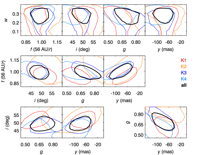
Figure 20: Visualization of the covariances between the model parameters $r,i,g,w,y$. The contours delineate the well-fitting solution family ($\chi^{2}\leq\chi^{2}_{\mathrm{min}}+\Delta\chi^{2}$) for each epoch, as well as for the combination of all four epochs. The strongest covariances are seen between ($f,y$) and ($y,g$).

Table 5: Correlation coefficients between pairs of model parameters in the brute-force grid-search study.

	$f$	$i$	$g$	$y$
$w$	$-0.08$	$-0.50$	$-0.50$	$-0.20$
$f$		$-0.15$	$-0.42$	$+0.72$
$i$			$+0.12$	$+0.30$
$g$				$-0.55$

We find the strongest covariance between ($f,y$). This positive covariance implies a negative covariance between ($r,y$), given that $f:=56\,\mathrm{AU}/r$. This behavior can be understood geometrically. The most prominent feature of the ADI images is the stark radial intensity gradient between the dark disk gap and the bright crescent of the forward-scattering near-side rim of the outer disk. As $y$ is made more negative, the disk center is shifted further away from the star, bringing the disk’s bright near side closer to the star. In order to keep the radial position of the gap edge in its observed location, the disk radius $r$ must increase to compensate. Decreasing the inclination $i$ provides another way to widen the projected disk gap along the $y$ axis and thus restore the position of the bright edge, but unlike a change in $r$, it changes the aspect ratio of the projected disk gap and thus degrades the fit to the curvature of the imaged bright crescent.

The strong negative covariances between ($f,g$) and ($g,y$) are more challenging to visualize. Decreasing $y$ and $f$ simultaneously, as discussed in the previous paragraph, should result in an overall widening of the bright crescent in the ADI image, even though its shape and location is roughly kept constant. This may then require an increase in forward-scattering efficiency $g$ to re-concentrate the flux in the central part of the crescent and thus restore the overall flux distribution.

In principle, observing the ansae and the far side of the gap edge would break these degeneracies. However, those features are not discernible in our current datasets. Next-generation high-contrast imaging facilities like SPHERE ZIMPOL will likely be capable of such observations (Thalmann et al., 2008; de Juan Ovelar et al., 2013).

6 Discussion

Overall, the disk architecture we derive from our near-infrared imaging data agrees well with the predictions from the SED (e.g., Espaillat et al., 2008) as well as millimeter and sub-millimeter interferometry (e.g., Piétu et al., 2007; Andrews et al., 2011). In the following subsections, we focus in particular on the disk aspects to which these previous methods of observations were insensitive, but which have become accessible through high-contrast imaging in reflected light.

6.1 Disk orientation (near vs. far side)

While the position angle of the projected system axis is easily measured in millimeter interferometry (Piétu et al., 2007) as well as near-infrared imaging (Paper I), it is more challenging to determine which of side of the disk is inclined towards the viewer. Mulders et al. (2010) proposed two possible architectures for the LkCa 15 system, both of which are compatible with the SED constraints, but which predict opposite brightness asymmetries between the near and far sides of the disk. In one scenario, the bright crescent observed in near-infrared imaging represents the directly illuminated far side of the gap wall, whereas the near-side wall is obscured by the bulk of the optically thick disk. In the second scenario, the observed crescent instead represents light forward-scattered off the near side of the outer disk rim, whose observable flux is greatly enhanced over the far side by anisotropic scattering. The far-side scenario is qualitatively supported by a disk modeling study by Jang-Condell & Turner (2013), whereas Piétu et al. (2007) and Grady et al. (2010) favor the near-side scenario based on asymmetries in the millimeter interferometry data and in space-based scattered-light images of the outer disk surface, respectively. Our first near-infrared imaging analysis in Paper I did not allow us to distinguish between these scenarios.

The quantitative approach presented in this work, however, clearly favors the near-side scenario. We achieve visually and numerically convincing fits to the data using disk models with a high Henyey-Greenstein factor of $g\approx 0.67$, which results in an extreme enhancement of the near-side reflected light over the far-side flux. Conversely, while we were also able to create an opposite brightness asymmetry using the far-side scenario, most of the scattered light is constrained to a narrow, self-shadowing gap wall, which fails to reproduce the radially extended morphology of the flux in our images (Figure 9).

We therefore conclude that the Northwestern side of the LkCa 15 disk is the near side, in agreement with Piétu et al. (2007) and Grady et al. (2010).

6.2 Dust grain properties

The derived value of the Henyey-Greenstein anisotropic scattering parameter $g\approx 0.67\leavevmode\nobreak\ [0.56,0.85]$ (cf. Fig. 17) can be used to estimate the size of the particles in the upper atmosphere of the disk, which are responsible for the scattering. Note that the inclination and opening angle of the LkCa 15 disk constrain the observable phase function to the range of scattering angles roughly from 34^∘ to 134^∘ (Fig. 21). For larger particles, the anisotropy typically increases, but most of this effect is concentrated at the smallest scattering angles (i.e., the full phase function is no longer well represented with a Henyey-Greenstein function). At intermediate angles, the phase function usually flattens and, for very large aggregates, becomes locally backward scattering (negative values of $g$; see e.g., Min et al., 2010, and Min et al. in prep). The rather large positive value of $g$ we find for LkCa 15 corresponds to particles that are roughly micron sized. This is in reasonable agreement with the grain sizes used in the upper atmosphere of our model disk, and it implies that these grains are not agglomerated in large aggregates.

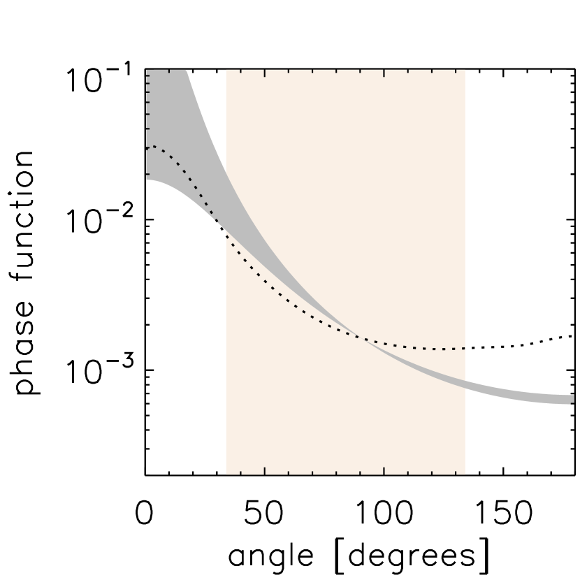
Figure 21: Phase functions of dust grains discussed in this work. Small angles are forward-scattering, large angles are backward-scattering. The gray region corresponds to the best fit range of the Henyey-Greenstein asymmetry parameter $g=[0.56,0.81]$. The dotted line is the phase function of the dust grains used for the SED fit. The orange region indicates the observable range of angles, 34^∘ to 134^∘.

6.3 Spatial asymmetry

In Paper I, we postulated a physical offset $x$ between the center of the LkCa 15 disk and the position of its host star along the line of nodes, based on the lateral asymmetry of the $H$-band ADI image. In our model, we included two free parameters $(x,y)$ to allow an arbitrary displacement of the center of the circularly symmetric model disk from the star, where $x$ is measured along the line of nodes (the major axis of the projected disk gap) and $y$ perpendicular to it (along the minor axis of the projected disk gap).

Our analysis of the new $K_{\mathrm{s}}$-band observations yielded consistently positive best-fit values of $x$ (cf. Fig. 7), tentatively confirming the existence of a lateral asymmetry in the appearance of the LkCa 15 disk. However, the absolute values of $x$ show a considerable spread, with the lower-quality epochs K2 and K4 supporting the large offset seen in Paper I, while the higher-quality epochs K1 and K3 advocate a much smaller offset consistent with zero. This may indicate that the real disk gap is roughly centered along the $x$ direction, and that a feature further out on the disk surface is responsible for the observed asymmetry. For instance, a spiral density wave extending beyond the western ansa could shift the perceived center of gravity of the disk flux towards that side, biasing the analysis towards positive $x$ values in the lower-quality datasets.

In addition, our analysis suggests a previously unknown and suprisingly large offset in the $y$ direction (cf. Fig. 18). Both the sign and the absolute value are consistent among all four $K_{\mathrm{s}}$-band epochs. Correcting for the foreshortening along the inclined disk plane, the best-fit offset of $-69$ mas translates to a physical displacement of $\sim$15 AU, corresponding to $\sim$0.3 times the gap radius.

This is a dramatic departure from the roughly symmetric disk architecture that has been assumed in all previous studies of LkCa 15, and thus we treat this result with caution until it can be independently confirmed. However, we note that a sizeable disk asymmetry could well have gone undetected in previous observations. Measurements of the system’s SED, as employed by Espaillat et al. (2008, 2010), are inherently insensitive to purely spatial information. While millimeter (Piétu et al., 2007) and submillimeter interferometry (Andrews et al., 2011) are capable of measuring disk information on large spatial scales at high S/N ratios, the stellar photosphere is invisible at those wavelengths, rendering a direct comparison of the disk and star positions impossible. Andrews et al. (2011) do not attempt to fit any such offsets in their data, but note that their disk center is $<70$ mas from the expected stellar position based on absolute pointing accuracy. This is marginally consistent with our best-fit offset. We also note that the near side of the disk appears brighter than the far side in Andrews et al. (2011), which is qualitatively expected if the near-side gap edge is closer to the star, and thus has a higher equilibrium temperature. Since millimeter interferometry traces thermal emission rather than reflected light, anisotropic scattering does account for this asymmetry.

Overall, our model treatment of the disk’s eccentricity – an azimuthally symmetric disk translated with respect to the star along the disk plane – is likely a simplification, whereas the real disk may have an elliptical gap, spiral arms, or even more irregular features (cf. HD 142527; Canovas et al. 2013). However, the fact that in our analysis all four epochs of observation consistently suggests a significant offset is a strong indication of an underlying physical asymmetry in the system architecture, regardless of its detailed morphology.

6.4 Wall shape

To date – and to our best knowledge – the shape of a transitional disk’s gap wall has only been detected in two other objects: HD 100546 (Panić et al., 2012; Mulders et al., 2013b) and TW Hya (Ratzka et al. 2007, Menu et al. in prep.), both with mid-infrared interferometry. In this work, we have inferred a wall-shape parameter of $w\approx 0.30$ for LkCa 15, which describes a gradual tapering of the outer disk surface density over a significant range of radii (a ‘round’ or ‘fuzzy’ wall) rather than a hard vertical cut-off ($w=0$). This value of $w$ is comparable to the wall shapes described for the previously mentioned targets, indicating that similar processes are likely at work shaping these walls. It should be noted, however, that steeper wall shapes in other objects might have escaped detection as there may be less of a difference observationally with the commonly assumed vertical wall. On the other hand, the missing cavities in the SEEDS survey (Dong et al., 2012) might be interpreted as extremely extended round walls.

A tapered surface density profile for LkCa 15 was also proposed by Isella et al. (2009), as a way of reconciling the millimeter flux deficit with the existence of a near-infrared excess, without invoking an additional inner disk component. However, it requires and extremely round wall ($w\gg 0.4$) to achieve sufficient optical depth in the inner regions to create a near-infrared excess, which is not supported by our observations. Even though the disk wall extends over a wide radial range (cf. Figure 5), the radiative transfer model requires an additional component to fit the near-infrared flux.

Since these pre-transitional disks (transitional disks with a near-infrared excess, implying the existence of an inner disk component at sub-AU radii) are thought to be shaped by planetary systems, rather than photo-evaporation, it is tempting to explain the the wall shape in terms of a planetary companion. Mulders et al. (2013b) have done so for HD 100546 using hydrodynamical models of planet-disk interactions, and found that the extreme roundness ($w\approx 0.35$) in this case is best explained by a brown dwarf companion. Taking their Figure 7 at face value, the well-fitting range of $w=[0.19,0.36]$ for LkCa 15 spans almost the entire plausible range of planet/star mass ratios, making it difficult to establish constraints on planet mass.

We note that planet mass also affects disk morphology in other ways, which we have not included in our model:

Gap depth.

While our imaging data confirm an abrupt drop in surface brightness inside the LkCa 15 disk gap, they do not exclude the presence of a residual level of dust in that area. Knowing the degree of dust depletion in the gap (the ‘gap depth’) would impose additional constraints on the planet mass. However, the oversubtraction effects generated during the ADI data reduction by the stark gradients of the nearby bright gap render an absolute calibration of the flux level in the gap extremely difficult. Deep polarimetric imaging, on the other hand, may provide access to this information in the near future.

Decoupling of gas and dust.

In contrast to HD 100546, the (sub)micron-sized dust grains in the disk wall of LkCa 15 show signs of dust settling (Espaillat et al., 2007; Mulders et al., 2010), indicating that they are dynamically decoupled from the gas and may be subject to radial drift, as in Pinilla et al. (2012b). This could alter the radial surface brightness/density profile of the disk, and potentially provide a better diagnostic for planet mass.

6.5 Constraints on planets and planet-induced dust grain differentiation

As explored in Pinilla et al. (2012b) and de Juan Ovelar et al. (2013), the presence of a planet in the disk generates a radial differentiation of dust grain sizes that is strongly related to the mass of the planet. The planet causes a pressure bump to form in the gas distribution of the disk, which traps large grains but allows for small grains to filter through towards smaller radii. As a result, the distribution of large grains exhibits a wider central gap than that of the small grains. Since NIR imaging and sub-mm interferometry mainly trace the micron- and mm-sized dust grains, respectively, this differentiation effect can be observed as a wavelength-dependent gap radius. Therefore, given the assumption that a single planet is responsible for the gap, the ratio of the gap radii measured at NIR and sub-mm wavelengths can be used to constrain the mass of the undetected planet (see Figure 8 in de Juan Ovelar et al. 2013). This scenario presents a plausible explanation for the “missing cavities” sample of the SEEDS survey (Dong et al., 2012) where no cavities were found in polarised intensity $H$–band images of sources displaying large cavities in sub-mm studies.

Our $K_{\mathrm{s}}$-band observations, the 870 $\mu$m observations presented in Andrews et al. (2011), and the SED fit carried out by Espaillat et al. (2010) all locate the wall at consistent radii of $r\approx[50$–$58]$ AU. LkCa 15 is therefore different in this regard from the “missing cavities” sources. This lack of dust grain size differentiation strongly suggests that the radial differentiation of dust grain sizes, if present, is not significant. Figure 8 of de Juan Ovelar et al. (2013) plots gap radius ratios between $R$-band and 880 $\mu$m as a function of planet mass. Preliminary calculations show that replacing $R$-band imaging with $K_{\mathrm{s}}$-band imaging does not significantly change this function. Taken at face value, gap radius ratios close to unity predict a mass of $M\lesssim 1\,M_{\mathrm{Jup}}$ for the planet responsible for the pressure distribution in the outer disc. In the case of a multi-planet system, this role is played by the outermost planet, as planets tend to influence the disk locally (Goodman & Rafikov, 2001).

It may be worth to note that the gap measured in the Andrews et al. (2011) study, at 870 $\mu$m ($\sim$50 AU), is the smallest of all gaps measured at different wavelengths which is interesting since the substellar companion scenario assumed by both Pinilla et al. (2012b) and de Juan Ovelar et al. (2013) causes the opposite effect (i.e. larger grains are further out). In their study Andrews et al. (2011) do mention that their uncertainties are underestimated which could bring the value closer to the ones obtained in e.g. Espaillat et al. (2010) and this study, however, if confirmed, this effect would require further investigation before any conclusions regarding the cause of this “reversed” dust grain size separation can be drawn.

Simulations show that a single companion would need to be very massive in order to open a gap as large as the one observed in the LkCa 15 disk ($M\gg 10\,M_{\mathrm{Jup}}$; Kraus & Ireland, 2012; Crida et al., 2006). Such a companion would be at odds with the lack of observable radial dust differentiation. However, a system comprising multiple low-mass planets could accommodate both of these constraints. Espaillat et al. (2008) note that the inner and outer boundaries of the gap in the LkCa 15 disk system are comparable to the smallest and largest orbital radii in our own planetary system, allowing for the the tantalizing possibility that the LkCa 15 system might be a young analog of our Solar System.

Kraus & Ireland (2012) propose a mass of $\sim$6 $M_{\mathrm{Jup}}$ for their planet candidate found in SAM observations. However, the authors note that this planet alone would be incapable of clearing the observed disk gap, necessitating a second, lower-mass planet in a wider orbit closer to the disk gap. Since this outer planet would dominate the radial dust differentiation, our findings do not contradict the existence of the proposed massive planet.

We cannot directly confirm or falsify the existence of the planet candidate reported by Kraus & Ireland (2012) from SAM observations in $L^{\prime}$ and $K$ band, since its separation from the star (70–100 mas) lies within the inner working angle of our ADI observations.

However, given the extreme anisotropy seen in our scattered-light images, the possibility should perhaps not be excluded that the disk itself may cause some of the structure seen in the SAM data, in a similar way as has been inferred for the similar case of T Cha (Olofsson et al., 2013).

6.6 Inner disk

As first described in Mulders et al. (2010), the nature of the inner dust component of the LkCa 15 pre-transitional disk affects the observational appearance of the outer disk, and can therefore be constrained by imaging observations of the outer disk. An optically thick inner disk would cast a shadow on the outer disk, whereas an optically thin dust shell would not. Espaillat et al. (2011) report a time variability in the spectrum of the LkCa 15 system in which the near- and mid-infrared fluxes exhibit negative covariance (‘see-saw effect’), which is taken as evidence for time-variable shadowing, and therefore supports the optically thick inner disk scenario.

The effective scale height of the inner disk $s$ is a free parameter in our model, thus our analysis is capable of detecting variable shadowing between epochs. Surprisingly, $\chi^{2}$ minimization of this parameter (cf. Section 5.5) consistently yields $s=0$ for all epochs, i.e., no shadowing is detected. This behavior can be explained either with the optically thin dust halo scenario (Mulders et al., 2010), with an optically thick inner disk tilted with respect to the outer disk, causing its shadow to miss the outer disk wall at most azimuths. Both explanations are, however, at odds with the ‘see-saw’ behavior observed in the mid-infrared, which implies a photometrically significant amount of shadowing on the outer disk. Although $s=0$ is a firm result of our analysis in all epochs, it is difficult to assess why the absence of a shadow increases the fit quality, and which model parameters could alleviate the need for a fully illuminated outer disk.

6.7 Remaining uncertainties

We caution that our forward-modeling analysis is limited by the extent of the disk model and its sampled parameter space. While we consider our best-fit models a convincing fit for our data, we acknowledge the possiblity that they may be approximations of a disk architecture beyond the scope of our model.

Next-generation adaptive-optics facilities may offer the means to reveal the structure of the LkCa 15 disk gap with more conservative high-contrast imaging methods, resolving these remaining uncertainties. Polarimetry is a particularly promising technique for such applications, as demonstrated by Quanz et al. (2013).

7 Conclusion

Following up on our $H$-band results from Paper I (epoch H1), we have obtained four new epochs of $K_{\mathrm{s}}$-band high-contrast direct-imaging observations of the LkCa 15 system in order to reveal new insights on the architecture of its pre-transitional disk. All four $K_{\mathrm{s}}$-band datasets (epochs K1–K4) were taken in consistent observing modes so as to enable direct comparison, using Gemini NIRI with pupil tracking to enable ADI data reduction.

In order to compensate for the known flux loss and morphological impact of ADI, we have performed an extensive forward-modeling analysis. By simulating a parametric grid of scattered-light images of disk models, forward-modeling them through the ADI process, and comparing the results to the observed ADI images with a $\chi^{2}$ metric, we have arrived at stringent quantitative constraints on the disk geometry.

These results are independent from, but consistent with, the constraints previously inferred from the system’s SED (Espaillat et al., 2010) and from (sub-)millimeter interferometry (Andrews et al., 2011). However, they also include new findings that have only become accessible through near-infrared high-contrast imaging:

• We find that the bright crescent seen in scattered-light ADI observations of LkCa 15 represents the strongly forward-scattering near side of the outer disk, rather than the far side (cf. Section 5.2).

• We tentatively confirm the existence of an asymmetry between the ansae as postulated in Paper I. Under the assumption that the disk can be described as azimuthally symmetric but physically displaced along the line of nodes (the major axis of the projected disk gap) by an offset $x$, we find consistently positive best-fit values for $x$ in all four $K_{\mathrm{s}}$-band epochs, in line with our H1 results (cf. Section 5.2). However, while the size of the best-fit $x$ offset is consistent with the H1 value in our lower-quality epochs K2 and K4, the higher-quality data of K1 and K3 indicate a much smaller offset consistent with zero. This may suggest that the observed asymmetry may be caused by a different mechanism than a displaced disk gap, such as perhaps by a spiral density wave beyond the western ansa of the disk gap, which may be mistaken for the disk gap in lower-quality data.

• Furthermore, our best-fit models exhibit a surprisingly large disk offset $y$ perpendicular to the line of nodes (along the minor axis of the projected disk gap), bringing the brightly illuminated near-side rim of the outer disk closer to the star (cf. Section 5.9). Unlike $x$, the values of $y$ are consistent with each other and significantly inconsistent with zero in all four $K_{\mathrm{s}}$-band epochs, lending the result credibility. While such a large displacement ($\approx$0.3 times the gap radius, deprojected) constitutes a dramatic departure from the symmetric architecture commonly assumed for LkCa 15, it could plausibly have escaped detection in SED and submillimeter interferometry. However, we note that a displaced circular gap is no longer a good approximation of an elliptical gap at an eccentricity of $e=0.3$, so the real shape of the LkCa 15 disk may well lie outside of the model parameter space considered in this analysis.

• We find evidence for a ‘round’ gap wall; i.e., a gradual rather than abrupt gradient of surface density between the gap and the outer disk, consistent with the wall being sculpted by a planetary companion (cf. Section 5.4).

• We obtain best results for a completely absent shadow from the inner disk on the outer disk wall (cf. Section 5.5). This may indicate that the inner disk is inclined with respect to the outer disk, causing its shadow to miss the outer disk at most azimuths.

The best-fit disk models are visualized in Figure 10, and the numerical results of the analysis are summarized in Table 3.

Finally, we acknowledge the fact that the results of our forward-modeling analysis are necessarily bound by the scope of the model and its parameter space, and that they are therefore simplistic approximations to the real, complex reality of the LkCa 15 disk. However, given the observational status quo, we consider them to represent the best estimate of the disk architecture to date.

In the near future, imaging polarimetry with next-generation adaptive optics facilities such as Subaru SCExAO (Guyon et al., 2011) or SPHERE ZIMPOL (Thalmann et al., 2008) may provide a more detailed view of the LkCa 15 disk with fewer model dependencies.

Appendix A Preliminary best-fit solutions

The parameter sets listed in Table 6 represent the preliminary, coarse model fits to our four observing epochs of LkCa 15 obtained through an iterative search during the early phase of this work. They are used as a starting point for the studies presented in Sections 5.2 and 5.5. Our final, optimized solutions and their confidence intervals are described in Section 5.3.

Table 6: Description of the preliminary best-fit (PBF) solutions to the four datasets.

Parameter	K1	K2	K3	K4
Scale factor $f$	0.93	1.00	1.00	0.97
Gap radius $r$ (AU)	52	56	56	54
Inclination $i$ (∘)	52	50	48	48
Henyey-Greenstein number $g$	0.60	0.80	0.70	0.60
Settling parameter $s$	0	0	0	0
Wall roundness $w$	0.25	0.35	0.25	0.30
Orientation angle $o$	147.7	150.5	150.7	150.7
Center offset $x$ (mas)	12	73	10	45
Center offset $y$ (mas)	$-68$	$-88$	$-84$	$-88$

Appendix B Best-fit solutions under the restriction of $\boldsymbol{y=0}$

Our analysis clearly favors a significant offset $y$ of the disk center perpendicular to the line of nodes (cf. Section 5.9). However, this offset is as of yet unconfirmed, and could therefore represent an unknown bias in our modeling approach. For this reason, we here provide an overview of how the imposed restriction of $y=0$ would affect our results.

Since some covariances are found between the parameters $r,i,g,w$ and $y$ (cf. Section 5.10), the $\chi^{2}$ plots for those parameters undergo significant changes. Figures 22–25 show the corresponding plots for the $y=0$ parameter sub-space.

In the unrestricted analysis, a range of $y$ values are included in the well-fitting family, each of which contributes a narrow valley to the $\chi^{2}$ landscape. For parameters that covary with $y$, the $\chi^{2}$ valleys change their positions with varying $y$, thus the final $\chi^{2}$ valley calculated over all $y$ is broadened. For this reason, imposing the restriction of $y=0$ results in steeper $\chi^{2}$ curves than in the unrestricted case.

Furthermore, since the natural best-fit value of $y$ is negative, the restriction of $y=0$ causes a negative [positive] shift in the best-fit value of parameters that exhibit positive [negative] covariation with $y$. The gap radius $r$ decreases from 56 AU to 50 AU, whereas the inclination $i$ rises from $50^{\circ}$ to $54^{\circ}$.

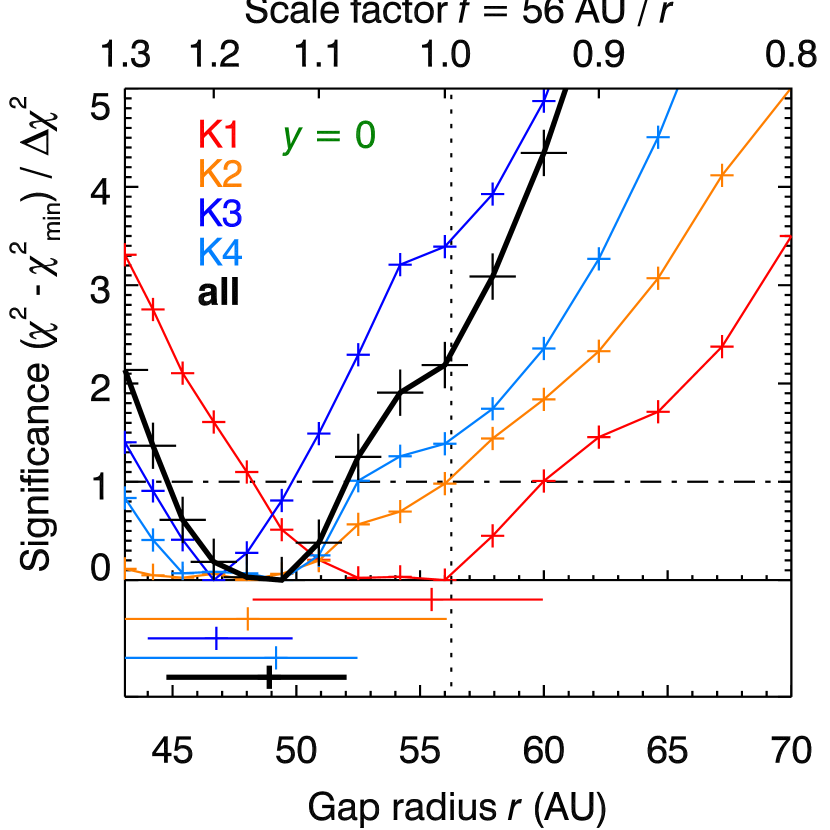
Figure 22: Constraints on the outer disk wall radius $r$ under the restriction of $y=0$. The plot shows the excess of the best-fit $\chi^{2}$ for a given $r$ with respect to the global minimum $\chi^{2}_{\mathrm{min}}$, normalized by the threshold value $\Delta\chi^{2}$. The color-coded curves represent each individual epoch, whereas the thick black curve is obtained by combining all four epochs. The dotted vertical line marks the best-fit value of $r$ from the unrestricted analysis. The bottom panel shows the well-fitting range and the best-fit value for all five analyses.

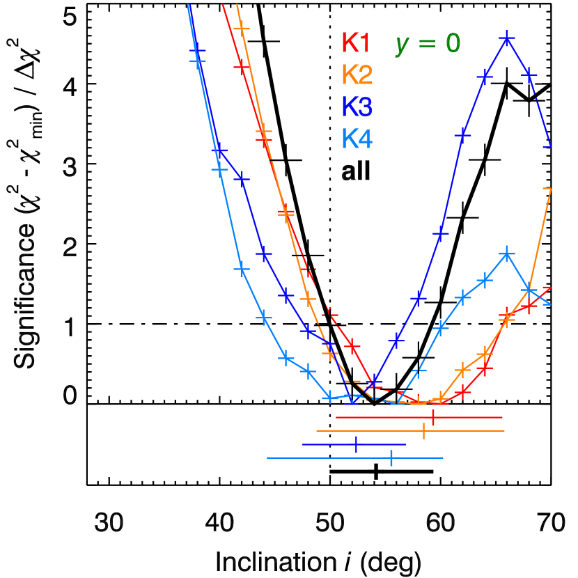
Figure 23: Constraints on the inclination $i$ of the disk plane under the restriction of $y=0$. The plot shows the excess of the best-fit $\chi^{2}$ for a given $i$ with respect to the global minimum $\chi^{2}_{\mathrm{min}}$, normalized by the threshold value $\Delta\chi^{2}$. The color-coded curves represent each individual epoch, whereas the thick black curve is obtained by combining all four epochs. The dotted vertical line marks the best-fit value of $i$ from the unrestricted analysis. The bottom panel shows the well-fitting range and the best-fit value for all five analyses.

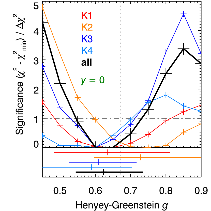
Figure 24: Constraints on the Henyey-Greenstein parameter $g$ under the restriction of $y=0$. The plot shows the excess of the best-fit $\chi^{2}$ for a given $g$ with respect to the global minimum $\chi^{2}_{\mathrm{min}}$, normalized by the threshold value $\Delta\chi^{2}$. The color-coded curves represent each individual epoch, whereas the thick black curve is obtained by combining all four epochs. The dotted vertical line marks the best-fit value of $g$ from the unrestricted analysis. The bottom panel shows the well-fitting range and the best-fit value for all five analyses.

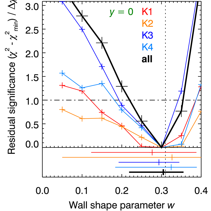
Figure 25: Constraints on wall shape parameter $w$ under the restriction of $y=0$. The plot shows the excess of the best-fit $\chi^{2}$ for a given $w$ with respect to the global minimum $\chi^{2}_{\mathrm{min}}$, normalized by the threshold value $\Delta\chi^{2}$. The color-coded curves represent each individual epoch, whereas the thick black curve is obtained by combining all four epochs. The dotted vertical line marks the best-fit value of $w$ from the unrestricted analysis, which coincide with the values obtained under $y=0$. The bottom panel shows the well-fitting range and the best-fit value for all five analyses.

Appendix C Exploration of disk wall scale height $\boldsymbol{h}$ as an additional free parameter

We ran a small-scale version of the brute-force parameter grid with outer disk scale heights $h=[1,2]$ in order to test whether the observed $y$ offset could be an aliasing effect of an inaccurate assumption on $h$. Since $h=1$ represents the hydrostatic equilibrium value, the test value of $h=2$ is an extreme case intended to probe the possible codependence of $h$ and $y$ with high sensitivity.

The analysis was run only for the best epoch, K3. We used the following parametric grid listed in Table 7. Its irregularity stems from the fact that it was assembled in two stages after it was found that the first stage did not fully encompass the best-fit solution.

Table 7: Parameter grid for the $h=2$ analysis.

$h$	=	[1,2]
$g$	=	[0.3, 0.5, 0.7, 0.8, 0.9]
$s$	=	[0, 1]
$w$	=	[0.05, 0.10, 0.15, 0.20, 0.30]
$i$	=	[40, 42, 44, 48, 52] deg
$f$	=	[0.933, 0.967, 1.000, …, 1.133]
$o$	=	preliminary best-fit values
$x$	=	preliminary best-fit values
$y$	=	$[-120,-110,-100,-90,-80,-60,-40,-20,0]$ mas

The best-fit solution was achieved for $g=0.70$, $s=0$, $w=0.05$, $i=44^{\circ}$, $f=1.067$, and $y=-90$ mas. The minimum $\chi^{2}$ achieved was 601, which is 2.8 $\Delta\chi^{2}$ above the $\chi^{2}_{\mathrm{min}}$ of the best-fit solution with $h=1$. While some of the best-fit parameters for $h=2$ deviate significantly from their $h=1$ counterparts (most notably the wall shape parameter $w$), we note that the best-fit value for $y$ is still in excellent agreement with the results for $h=1$ ($y=-70\leavevmode\nobreak\ [-115,-45]$ mas). This implies that there is no significant covariance between $y$ and $h$.

This behavior can be understood in conjunction with the fact that the best-fit models do not include a shadow from the inner disk on the wall of the outer disk ($s=0$), and thus the wall appears as a single bright crescent rather than two distinct thin arcs. Increasing the outer disk scale height $h$ makes the crescent wider (thus perhaps explaining the reduction in the wall shape parameter $w$, which is responsible for widening the crescent in the global best fit with $h=1$), but does not affect its overall position.

Thus, we conclude that the observed offset in $y$ is a robust result of our analysis within the framework of our disk model, and does not reflect an underlying error in the outer disk scale height $h$. We continue to use $h=1$ as a fixed internal parameter for this work.