Anisotropic expansion and SNIa: an open issue

Abstract

We review the appropriateness of using SNIa observations to detect potential signatures of anisotropic expansion in the Universe. We focus on Union2 and SNLS3 SNIa datasets and use the hemispherical comparison method to detect possible anisotropic features. Unlike some previous works where non-diagonal elements of the covariance matrix were neglected, we use the full covariance matrix of the SNIa data, thus obtaining more realistic and not underestimated errors. As a matter of fact, the significance of previously claimed detections of a preferred direction in the Union2 dataset completely disappears once we include the effects of using the full covariance matrix. Moreover, we also find that such a a preferred direction is aligned with the orthogonal direction of the SDSS observational plane and this suggests a clear indication that the SDSS subsample of the Union2 dataset introduces a significant biased, making the detected preferred direction unphysical. We thus find that current SNIa surveys are inappropriate to test anisotropic features due to their highly non-homogeneous angular distribution in the sky. In addition, after removal of the highest inhomogeneous sub-samples, the number of SNIa is too low. Finally, we take advantage of the particular distribution of SNLS SNIa sub-sample in the SNLS3 data set, in which the observations were taken along 4 different directions. We fit each direction independently and find consistent results at the 1$\sigma$ level. Although the likelihoods peak at relatively different values of $\Omega_{m}$, the low number of data along each direction gives rise to large errors so that the likelihoods are sufficiently broad as to overlap within 1$\sigma$.

I Introduction

Recent results from the Planck mission (Planck, ) have strengthened the status of the $\Lambda$CDM model (LCDM, ) as the standard cosmological model driving the dynamics of our Universe. This evidence should not be lightly assumed though, as the $\Lambda$CDM model implicitly requires the validity of a large number of assumptions: the Cosmological Principle (CosmoPrinciple, ), i.e., that our Universe is homogeneous and isotropic on sufficiently large scales; the full validity of General Relativity all the way up to the horizon scale; the existence of unknown dark matter to grow structures via gravitational collapse; the presence of an unnaturally small cosmological constant, which drives the present acceleration of our Universe; and a nearly scale invariant gaussian primordial spectrum of perturbations generated during an inflationary epoch in the early universe. Each of them might be individually questioned (AgainstLCDM, ). Among them, we will focus here on he validity of the Cosmological Principle and analyse the possibility of detecting a certain amount of anisotropy by using SNIa observations.

Theoretically motivated models giving rise to a violation of the Cosmological Principle by inducing a late-time anisotropic expansion of the universe have been extensively considered in the literature. In Campanelli:2006vb , it was argued that the presence of large scale (homogeneous) magnetic fields Campanelli:2006vb could induce a certain level of eccentricity in the universe expansion that might even solve the low CMB quadrupole problem. The same kind of anisotropic expansion can be achieved by assuming that the dark energy large scale rest frame might differ from that of radiation and/or matter, giving rise to a cosmology with moving fluids. Within this scenario, the dipole acquires a cosmological contribution MovingDipole , the CMB quadrupole is also modified because the relative motion introduces a certain level of eccentricity Beltran Jimenez:2007ai and large scale flows of matter are generated Jimenez:2008vs . The possibility of having different large-scale frames for dark matter and dark energy has also been considered more recently in Harko:2013wsa . Another scenario with anisotropic expansion was proposed in Rodrigues:2007ny , where the effects of having an anisotropic cosmological constant was studied. More generally, models with anisotropic dark energy Koivisto:2007bp ; Battye:2006mb ; Campanelli:2011uc ; Linder or anisotropic curvature Koivisto:2010dr have also been considered.

Most of the models leading to anisotropic expansion discussed in the previous paragraph make the universe metric be of the Bianchi I type, that is, the universe expands at different rates along the 3 spatial directions. Some of those models are characterized by the presence of a privileged direction, which is identified with the vector characterizing the model, direction of the magnetic field, direction of the relative motion between different species. In these cases, the metric is restricted to be of the axisymmetric Bianchi I type in which the expansion rate along the privileged axis differs from the expansion rate along the orthogonal directions. Of course, the amount of anisotropy that these models can generate while being compatible with the highly isotropic CMB is tightly constrained. The main effect comes from the Integrated Sachs-Wolf effect, which is an accumulative effect from the last scattering surface until today. Thus, for models with a non-dynamical evolution of the eccentricity like models with anisotropic equation of state, such anisotropy is essentially constrained to be less than $\mathrel{\mathop{\kern 0.0pt\hbox to0.0pt{\raise 0.86108pt\hbox{$<$}\hss}}\lower 3.87495pt\hbox{\kern-1.90002pt$\sim$}}10^{-4}$ Appleby:2009za . However, if the source of anisotropy is dynamical or there are compensating effects, the constraints are less stringent. In fact, having a period of anisotropic expansion at low redshift would mainly affect the CMB quadrupole, which is affected by a large cosmic variance so that it has less constraining power than the higher multipoles.

Observations of SNIa have been proposed and used as probes of large scale anisotropies. One of the first attempts to constrain the isotropy of the universe by resorting to SNIa measurements was made in Kolatt:2000yg . In Bonvin:2006en the luminosity-distance dipole from the SNIa distribution was analysed and shown how to use it to obtain measurements of the Hubble expansion rate $H(z)$. Higher multipoles and additional contributions to the luminosity distance were subsequently computed dLanisotropies . SNIa measurements have also been used to study the isotropy of the Hubble diagram Schwarz:2007wf , local bulk flows bulkflowsSN , the matter distribution Antoniou:2010gw or the potential anisotropy of the deceleration parameter Cai:2011xs . The possibility of constraining dark energy fluctuations by means of the luminosity distance was explored in Blomqvist:2010ky . In Mariano:2012wx , a dipole-like distribution for dark energy was analyzed along with its possible correlation with the fine structure dipole. Also a dipole-like distribution was considered in Cai:2013lja , but applied to the luminosity distance with respect to the $\Lambda$CDM case. A fully Bayesian tool to search for systematic contamination in SnIa data was developed in Amendola:2012wc and further extended, including searches for anisotropic signals, in Heneka:2013hka .

In the present work we will revisit the constraints that can be obtained on the anisotropy of the universe from SNIa observations. We shall mainly follow the same approach as in Antoniou:2010gw where the authors used a certain version of the hemispherical comparison method to test the isotropy of the matter distribution at the background (homogeneous) level. We intend to refine their approach by including some influential subtleties concerning the SNIa observations. In particular, we show that including the full covariance matrix with the corresponding increase in the errors makes the significance of previously claimed preferred direction detections disappear. Moreover, we will show that such potential (although not statistically significant) preferred direction happens to be be aligned with the orthogonal direction to the plane of observation of the SDSS subsamples, being an indication of its biased origin due to the particular observation strategy (i.e., of its highly clustered angular distribution along only four directions in the sky) of such a subsample.

The paper is organized as follows: in §. II we will describe the SNIa samples we have chosen for our analysis and their main properties; in §. III we will describe the original method we use to test the presence of anisotropic expansion and the main novelties we introduce; in §. IV we apply our method to a set of simulated data with a known anisotropic distribution in order to test its validity; in §.V we finally show the results obtained from our analysis and in §.VI we conclude by discussing our results.

II SNIa data

This Section will be devoted to introducing the SNIa datasets that we will use later on for our analysis. We will discuss the $\chi^{2}$ estimator to be used when using SNIa as well as some useful properties of our cosmological data sample which should be taken into account in order to obtain correct results.

The most updated SNIa samples so far are SNLS3 SNLS provided by the SuperNova Legacy Survey team and Union2 Union2 provided by the SuperNova Cosmology Project team. A newer collection of SNIa from the Union team is available and called Union2.1. It has $23$ more SNIa with respect to its predecessor. However, we prefer to use the Union2 compilation in favour of making the comparison with older literature easier and more direct. Also, Union2.1 only adds $\approx 23$ SNIa, so we expect their statistical weight for our analysis to be not very significant. There is also a recent compilation with 112 new SNIa provided by the Pan-STARRS1 Medium Deep Survey team Rest:2013bya , which we will not use because it has a non-homogeneous angular distribution (see Table.1 from Rest:2013bya ), which makes it unsuitable for testing anisotropy. It is worth stressing here nevertheless that we aim to testing the suitability of current SNIa datasets to seek for anisotropic features and we do not intend to obtain the most updated constraints on them (since, as we will show, current datasets are actually unsuitable for that purpose).

II.1 Statistical background

The $\chi^{2}$ estimator for SNIa observations is generally defined as

$$\chi^{2}=\Delta\boldsymbol{\mathcal{F}}\;\cdot\;\mathbf{C}^{-1}\;\cdot\;\Delta\boldsymbol{\mathcal{F}},\;$$ (1)

where $\Delta\boldsymbol{\mathcal{F}}=\mathcal{F}_{theo}-\mathcal{F}_{obs}$ is the difference between the observed and theoretical value of the observable quantity, $\mathcal{F}$, and $\mathbf{C}^{-1}$ is the inverse of the covariance matrix. For the SNLS3 compilation, the observable quantity $\mathcal{F}$ will be the SNIa magnitude $m_{mod}$ for SNLS3, defined by

$$m_{\rm mod}=5\log_{10}[d_{L}(z;c_{i})]-\alpha(s-1)+\beta\mathcal{C}+\mathcal{M}\;.$$ (2)

In this expression, the $c_{i}$ denote the set of cosmological parameters that are to be fitted, $\mathcal{M}$ is a nuisance parameter combining the Hubble constant $H_{0}$ and the absolute magnitude of a fiducial SNIa and $d_{L}$ is the dimensionless luminosity distance:

$$d_{L}(z,c_{i})=(1+z)\ \int_{0}^{z}\frac{\mathrm{d}z^{\prime}}{E(z^{\prime},c_{i})}\;,$$ (3)

with $E(z)$ the dimensionless Hubble expansion function $H(z,c_{i})/H_{0}$.

The SNLS3 team also provides the full multidimensional covariance matrix with statistical and systematic errors for all the physical quantities involved in their analysis, assuming $\alpha$ and $\beta$ as free fitting parameters:

$$\mathbf{\widehat{C}}=\sigma^{2}_{stat}\mathbf{\widehat{I}}+\mathbf{\widehat{v}_{0}}+\alpha^{2}\mathbf{\widehat{v}_{a}}^{2}+\beta^{2}\mathbf{\widehat{v}_{b}}^{2}+2\alpha\mathbf{\widehat{v}_{0a}}-2\beta\mathbf{\widehat{v}_{0b}}-2\alpha\beta\mathbf{\widehat{v}_{ab}}\;$$ (4)

with

$$\sigma^{2}_{stat} = \sigma_{mB}^{2}+\alpha^{2}\sigma_{st}^{2}+\beta^{2}\sigma_{col}^{2}+2\alpha\sigma_{ms}-2\beta\sigma_{mC}$$ (5)

$$- 2\alpha\beta\sigma_{sC}+\sigma_{int}^{2}+\sigma_{z}^{2}+\sigma_{pec}^{2}$$

the diagonal elements of the statistical errors, which are respectively: errors on magnitude; errors on stretch; errors on color; correlations between magnitude and stretch, magnitude and colors, stretch and colors; intrinsic dispersion errors; redshift errors; peculiar velocity errors; and: $\widehat{v}_{0}$ the out-of-diagonal statistical and systematic errors on magnitude; $\widehat{v}_{a}$ the same for the stretch; $\widehat{v}_{b}$ for the color; $\widehat{v}_{0a}$ for the correlation between magnitude and stretch; $\widehat{v}_{0b}$ for the correlation between magnitude and color; $\widehat{v}_{ab}$ for the correlation between stretch and color. In (SNLS, ) it is also argued that a correlation between SNIa magnitude and the mass of the host galaxy might be present. To account for this effect, they propose to divide the total sample into two groups: SNIa whose host galaxy mass is $<10^{10}$ $M_{\odot}$ and SNIa with galaxy mass $>10^{10}$ $M_{\odot}$. This division influences the definition of the $\chi^{2}$; see the appendix of (SNLS, ) and the two $\mathcal{M}$ values marginalization formulae that we will adopt for SNLS3.

On the other hand, the Union2 compilation observable is the distance modulus $\mu$, defined by

$$\mu\equiv m_{\rm mod}-M=5\log_{10}[d_{L}(z,c_{i})]+\mu_{0}\;,$$ (6)

where $M$ is the absolute magnitude and $\mu_{0}$ is a nuisance parameter similar to SNLS3 parameter $\mathcal{M}$. The main difference with SNLS3 is that the $\alpha$ and $\beta$ parameters are fixed at a preliminary stage (Union2, ) and the given full covariance matrix does not depend on them. Union2 files lack of the necessary data to distinguish the two host galaxy mass families, so that we will use the one-$\mathcal{M}$ value marginalization formulae in (SNLS, ).

II.2 Angular distribution

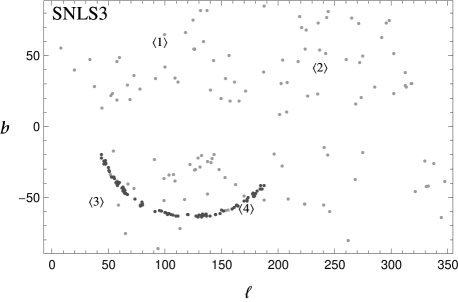
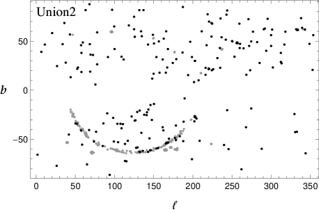
Figure 1: SNIa sky distribution in galactic longitude $l$ and latitude $b$. Left panel. SNLS3 SNIa sample: light grey points are Low-z SNIa; and Hubble data set; black points are SDSS SNIa; numbers in bracket are SNLS3 SNIa pointing toward different directions of the sky. Right panel. Union2 SNIa sample: light grey points are from SDSS, SNLS and smaller sub-samples with a not-homogeneous distribution in the sky; black points constitute the cut Union2 sample and highlight sub-sample from the total Union2 data set which show an homogeneous distribution in the sky.

Since the main aim of the present work is testing the isotropy of SNIa samples, it is important to perform a preliminary analysis of the angular distribution of the samples that we are going to use. This is important since one could encounter cases with a false detection of a preferred direction in the universe, whose actual underlying reason might be a non-homogeneous angular distribution of the sample. We also stress here that no tomographic analysis considering redshift distribution of SNIa will be performed in this work. Even if possible, it would reduce the number of SNIa data in each redshift bin, thus reducing the predictive power with too large errors on the cosmological parameters. We implicitly assume that the SNIa properties do not evolve throughout the expansion of the universe (at least for low redshifts where the SNIa are observed), but studying redshift-dependences of intrinsic SNIa properties is beyond the scope of the present work. We also comment here in advance that the main problem (discussed in next sections) will be related to the angular distribution of SNIa in the Union2 and SNLS3 datasets (mainly due to the fact that the SDSS sub-sample only gives data along 4 specific directions in the sky).

The SNLS3 sample is made out of four smaller sub-samples from four different surveys SNLS : Low-z, SDSS, SNLS and SNIa from the Hubble Telescope. In the left panel of Fig. 1 we show in galactic coordinatesthe position of each SNIa in the sky , the longitude $l$ and the latitude $b$. SNIa from Low-z and Hubble samples are shown in light grey; SDSS SNIa are shown in black; SNLS SNIa are identified by numbers in brackets. SDSS SNIa are distributed in the region scanned by the SDSS survey and specifically chosen for the supernova survey project SDSS . On the other side, SNLS SNIa show a beam distribution: all ($242$) them are concentrated in four beams pointing toward different directions of the sky. Clearly, this is a counter intuitive property which makes them unsuitable to be used in our analysis (this was also pointed out in (Schwarz:2007wf, ) where the authors referred to the very predecessor of this latest sample). However, this sample is specially suited for the approach suggested in Linder , since one can determine the cosmological parameters along the four different directions independently. We will perform this analysis in §. V.3.

In the right panel of Fig. 1 we show the Union2 sample distribution in sky. It shares many objects in common with the SNLS3 sample, but with the addition of many smaller sub-samples. We still have SDSS and SNLS sub-samples in it, clearly identified in light grey circles.

Based on these considerations, and in order to develop our analysis, we will perform our statistical study considering two samples: the total Union2 data set; and the so-called cut Union2 one, which will correspond to the black points in Fig. 1. The cut sample is obtained considering only sub-samples which show an homogeneous distribution in space, so that, for example, SDSS, SNLS and others which have a peculiar angular distribution are not considered. The cut sample will be made of $226$ SNIa, approximately the $40\%$ of the total sample. The cut-criterium has not been arbitrarily chosen but it is well-motivated by the results we will show in next sections, essentially consisting in removing the highly inhomogeneous subsamples.

Finally, we underline another important property of the SNIa distribution: the lack of observations in a narrow region about the galactic plane, clearly identified by the condition $b=0$. Both SNLS3 and Union2 data sets show a void in the region $-15\lesssim b\lesssim 15$; this is a consequence of the obscuration from excessive stellar density in such direction, and it is a problem that cannot be overcome in any way in this case.

III Hemispherical comparison method

This method was already used to look for asymmetries in the CMB in Eriksen:2003db , where the hemispherical asymmetry anomaly was discovered. More recently, it has also been used to look for evidences of anisotropic features in the Hubble diagram Schwarz:2007wf , whereas a different version of it was used in Antoniou:2010gw . We will adopt the approach used in the latter.

The main idea behind it is to split the celestial sphere into two hemispheres and fit the corresponding cosmological data sets for each hemisphere independently. The two hemispheres are determined by the corresponding equatorial plane identified, in our analysis, by the vector orthogonal to such a plane, with galactic longitude $l_{a}$ and latitude $b_{a}$. Then, one looks for the splitting that yields the maximum difference for the cosmological parameters of the best fit on each hemisphere. It is maybe convenient to stress that this method is simply designed to look for anisotropic features within a given data set of cosmological observations, but it does not imply a direct link with the true universe model.

Obviously, this procedure will always give a maximum difference direction, and one should study then the statistical significance of such detection as compared to the expected level of anisotropy in a pure isotropic model (that will always have some anisotropy due to statistical fluctuations). In Antoniou:2010gw , the authors fit the SNIa of each hemisphere to two independent $\Lambda$CDM models with vanishing spatial curvature and two different matter density parameters. Then, they search for the direction that maximizes the quantity

$$\frac{\Delta\Omega_{m}}{\overline{\Omega}_{m}}\equiv 2\frac{\Omega_{m}^{N}-\Omega^{S}_{m}}{\Omega_{m}^{N}+\Omega^{S}_{m}}$$ (7)

where $\Omega_{m}^{N,S}$ correspond to the values of $\Omega_{m}$ for the North and South hemispheres with respect to the chosen equatorial plane. This quantity can be interpreted as a normalized difference between both values of $\Omega_{m}$. In Antoniou:2010gw , the authors actually do not look for the maximum of this quantity. Instead, they generate a certain number of random directions in the sky ($400$ directions for the Union2 data set, with about $280$ SNIa per hemisphere) and consider the maximum value of $\frac{\Delta\Omega_{m}}{\overline{\Omega}_{m}}$ among the random distribution of generated directions. In this work we aim at revisiting this problem by making subtle methodological differences, which we describe and justify below, from which expectably more refined conclusions will emerge and which, why not, will perhaps eventually lead to different conclusions. Specifically, in this work we will consider the following points:

• We will assume that each hemisphere is well-described by a $\Lambda$CDM model, although they might have a different matter density, $\Omega_{m}$. Despite the availability of more complex cosmological models involving a larger number of theoretical parameters, this choice seems a reasonably minimal extension and appropriate for our purposes.

• The main difference from previous works (specially with Antoniou:2010gw ) will be the use of Monte Carlo Markov Chain (MCMC) methods for the statistical analysis. After having split the data into two hemispheres, we will not select a certain amount of random directions but, instead, we will use an MCMC method to explore the entire space parameter and to obtain an angular map of the $\chi^{2}$ function. Then, we will be able to conclude which is the preferred direction of anisotropy of our SNIa sample, if any.

We will minimize the $\chi^{2}$ estimator using MCMC methods and testing their convergence with the power spectrum algorithm defined in (Dunkley05, ). In the case of the hemispherical comparison method, such an estimator is defined as explained in detail in the previous Section with the following Hubble expansion rate:

$$E(z)=\left\{\begin{array}[]{ll}\left[\Omega_{m}^{N}(1+z)^{3}+(1-\Omega_{m}^{N})\right]^{1/2},&\text{if}\;\hat{r}\cdot\hat{r}_{i}>0\\ \left[\Omega_{m}^{S}(1+z)^{3}+(1-\Omega_{m}^{S})\right]^{1/2},&\text{if}\;\hat{r}\cdot\hat{r}_{i}<0\end{array}\right.$$ (8)

where

$$\hat{r} = (\cos l_{a}\cos b_{a},\sin l_{a}\cos b_{a},\sin b_{a})$$

$$\hat{r}_{i} = (\cos l_{i}\cos b_{i},\sin l_{i}\cos b_{i},\sin b_{i})\;,$$ (9)

are the directions identifying the equatorial plane and the directions of each SNIa in the sample, respectively, with $(l,b)$ the corresponding galactic coordinates. Of course, the $\Lambda$CDM model and spatial flatness are assumed in each hemisphere. This assumptions might be dropped and more general cases could be considered. The simplest step further could be the addition of an anisotropic dark energy equation of state parameter $w$ (Linder, ), but this is out of the purpose of this work. Moreover, present data sets comprise too few SNIa already for the simplest case, so even poorer constraints will be obtained if we allow for additional free parameters.

It is worth to point out here that MCMC methods give us the possibility to easily implement priors on fitting parameters, if any physically well motivated reason is for them. In our analysis, we have left the cosmological parameters $\Omega_{m}^{N}$ and $\Omega_{m}^{S}$ free to span the range $[0,1]$ with no other requirement. On the other hand, the equatorial planes coordinates $l_{a}$ and $b_{a}$ can be constrained to a certain range due to evident symmetries considerations; we chose the ranges $0$°$\leq b_{a}\leq 90$°  and $0$°$\leq l_{a}<360$°. This last point has to be investigated in detail, as long as we do not know the degree of suitability of MCMCs for such a test. The main parameters to be fit here will be the two cosmological values of $\Omega_{m}$, namely $\Omega_{m}^{N}$ and $\Omega_{m}^{S}$, and the two equatorial plane coordinates, i.e. $l_{a}$ and $b_{a}$. While it is well known the way $\Omega_{m}^{N}$ and $\Omega_{m}^{S}$ are related to observations and theory, this is not the same for the equatorial plane coordinates. $\Omega_{m}^{N}$ and $\Omega_{m}^{S}$ are smoothly varying quantities, in the sense that $\chi^{2}$ varies smoothly when they are changed; on the other hand, a change in $l_{a}$ and $b_{a}$ might not be related to a change in $\chi^{2}$ for a given dataset. Depending on the spatial distribution of SNIa, there are voids in the SNIa distribution because of the few number of SNIa available for the whole sky, so that any value of $l_{a}$ and $b_{a}$ in that range would give the same result. In other words, for changes in $(l_{a},b_{a})$ such that the number of supernovae on each hemisphere remains the same, $\chi^{2}$ will not vary.

If we wanted to perform an analysis similar to (Antoniou:2010gw, ), we should use MCMC to minimize $\chi^{2}$ in each random direction as the authors do; but this would not bring any novelty to the topic. Here instead, we let the MCMC explore freely all the parameter space, obtaining a full-sky angular $\chi^{2}$ distribution, from which we can derive the probability distributions of all the theoretical parameters involved. In other words, even if the MCMC will jump in a discrete way from one point to another, it will be the closest-to-continuous exploration method of the space parameter that can be realized in a non-hardware/time consuming effort. Notice that the MCMC will allow to refine the search as much as necessary.

As a further difference with previous works in the literature, we will use the full statistical plus systematic non-diagonal covariance matrix error for SNIa. As we will show, this will impact crucially the corresponding findings. In (Antoniou:2010gw, ) each hemisphere was independently fitted, i.e., the total $\chi^{2}$ was obtained as the sum of the two independent contributions obtained for each hemisphere $\chi^{2}_{\rm full\;sky}=\chi^{2}_{\rm north}+\chi^{2}_{\rm south}$. This approach was possible because the considered covariance matrix was diagonal, thus allowing the separation of the $\chi^{2}$ in the northern and southern terms so that minimization of each one can be independently performed. However, the use of only diagonal terms of statistical errors is well-known to produce a large underestimation of errors on cosmological parameters (up to $\approx 70\%$, see (SNLS, )) and might also produce a bias in the detection of an eventual anisotropy. Moreover, the independent fit of each hemisphere is not strictly correct, because another well-known effect is that SNIa are strongly correlated with each other thus resulting in a non-diagonal covariance matrix, which will play a crucial role for the significance of possible anisotropic features. Finally, in (Antoniou:2010gw, ), the parameter used to define the $1\sigma$ confidence levels of the equatorial plane direction is strongly related to the errors on cosmological parameters (see their Eq. (2.11)). It is thus clear that any larger contribution to such errors will produce larger errors for the equatorial plane coordinates, and so a less established detection of anisotropy. Having stablished the main lines of revision we continue to describe the setup still following the mentioned main references.

IV Analysis: preliminary tests

Table 1: MCMC results.

mock I : known anisotropy vs homogeneous angular distribution
mock	$(\Omega_{m}^{N}-1\sigma,\Omega_{m}^{N}+1\sigma)$	$(\Omega_{m}^{S}-1\sigma,\Omega_{m}^{S}+1\sigma)$	$(l_{a}-1\sigma,l_{a}+1\sigma)$	$(b_{a}-1\sigma,b_{a}+1\sigma)$
total diag (I)	$(0.520,0.586)$	$(0.064,0.099)$	$(133.81$°$,138.01$°)	$(26.43$°$,27.64$°)
total cov (I)	$(0.479,0.581)$	$(0.048,0.098)$	$(133.62$°$,137.51$°)	$(26.49$°$,27.62$°)
cut cov (I)	$(0.509,0.744)$	$(0.041,0.154)$	$(121.64$°$,147.97$°)	$(22.64$°$,39.95$°)
real data: unknown anisotropy vs real angular distribution
real	$(\Omega_{m}^{N}-1\sigma,\Omega_{m}^{N}+1\sigma)$	$(\Omega_{m}^{S}-1\sigma,\Omega_{m}^{S}+1\sigma)$	$(l_{a}-1\sigma,l_{a}+1\sigma)$	$(b_{a}-1\sigma,b_{a}+1\sigma)$
tot diag	$(0.239,0.287)$	$(0.257,0.310)$	$(0$°$,360$°)	$(0$°$,90$°)
tot cov	$(0.215,0.313)$	$(0.251,0.354)$	$(0$°$,360$°)	$(0$°$,90$°)
cut cov	$(0.208,0.302)$	$(0.363,0.550)$	$(132.16$°$,152.84$°)	$(26.39$°$,27.83$°)

Prior to the application of the method to real data, we will first study and assess the following relevant aspects:

• Suitability of MCMCs for anisotropy detection.

• Degradation in the anisotropy signal due to the use of the full covariance matrix error.

• Degradation in the anisotropy signal due to galactic plane.

The first point to be addressed is whether the use of MCMC is effectively suitable to look for a certain level of anisotropy in the SNIa distribution. For that, before using real SNIa data sets, we will apply our algorithm to a set of simulated data with a homogeneous distribution in the sky data set of supernovae. We will endorse this simulated data with a known anisotropic signal as follows: We will demand a preferred direction determined by $\hat{r}$ and given by the equatorial plane galactic coordinates $l_{a}=136.84$°  and $b_{a}=27.07$°. This plane came out as the preferential plane when the MCMC analysis was applied to the cut Union2 sample when the full covariance matrix error is used (see following sections). Then, we generate a homogeneous set of random vectors $\hat{r}_{i}$ that will give the distribution of the SNIa in the sky. With this distribution, we confer each SNIa a distance modulus following the $\Lambda$CDM model given in Eq. (8), where we chose $\Omega_{m}^{N}=0.5$ and $\Omega_{m}^{S}=0.1$, and assuming that the Hubble constant is $H_{0}=72$ km s^-1 Mpc^-1. All the other quantities needed, namely, redshifts and covariance matrix errors, are assumed to be exactly equal to those of the real Union2 dataset.

Another issue that we want to study is the following. Given that our galaxy prevents us from having observations of SNIa near the galactic plane (or, equivalently, a lack of data points around that plane with respect to the rest of the sky) we want to explore also whether the absence of SNIa data in the region near the galactic equator can introduce a potential bias or not. In particular, if the anisotropy happens to be aligned with the galactic plane, this will certainly contribute to increase the errors in the position of the preferred axis. To study this effect we will use the mock SNIa sample described above and will remove all the SNIa in the range $-10$°$<b<10$°  around the galactic plane, and we will redistribute them outside that band.

Results are in Table 1. We compare three cases:

1. the total mock Union2 sample with homogeneous distribution and diagonal-only errors (named mock total diag (I));

2. the total mock Union2 sample with homogeneous distribution and full covariance matrix (named mock total cov (I));

3. the cut mock Union2 sample with homogeneous distribution, the galactic plane cut applied, and full covariance matrix (named mock cut cov (I))

We can point out the following results:

• A homogeneously distributed sample is, of course, the perfect ideal case for a clear detection of an anisotropy signal.

• A more important point is that the MCMC method reveals to be fully suitable for our scopes: In all the cases considered the direction and the amount (different $\Omega_{m}$ values) of the anisotropy signal are quite clearly detected. We note, however, that even in this case there is an obvious degradation of the anisotropy signal, intrinsically due to the dispersion of data and to the observational errors. Indeed, such a degradation will make the detection in real data not very statistically significant.

• The use of diagonal-only errors or of the full covariance matrix influences only the amount of anisotropy, not its direction. We can easily see that the $1\sigma$ confidence interval for $\Omega^{N}_{m}$ and $\Omega^{S}_{m}$ is $\approx 65\%$ larger than the diagonal-only errors case when the full covariance matrix errors is used.

• The direction of anisotropy is much more related to the number of SNIa included in the sample. This is clearly shown by comparing the total ($557$ SNIa) and the cut ($226$ SNIa) cases. We note that the cut sample is derived assuming the lack of SNIa around the galactic plane too. Thus, less SNIa and the observational void around the galactic plane can: double the $1\sigma$ confidence interval of $\Omega^{N}_{m}$ and $\Omega^{S}_{m}$; and enlarge the $1\sigma$ confidence interval of equatorial plane coordinates, $l_{a}$ and $b_{a}$, of $\approx 10$ times.

V Analysis: results

Now that we have proved the suitability of the MCMC method by applying it to simulated data, we shall turn to real data. We shall first look at the Union2 compilation. We have applied the hemispherical comparison method and run a series of MCMC chains to obtain the best fit in three cases:

1. the total real Union2 sample with diagonal-only errors as in (Antoniou:2010gw, ) (named real total diag);

2. the total real Union2 sample with full covariance matrix (named real total cov);

3. the cut real Union2 sample with full covariance matrix (named real cut cov);

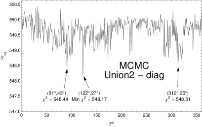
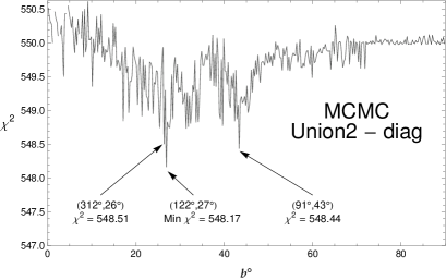
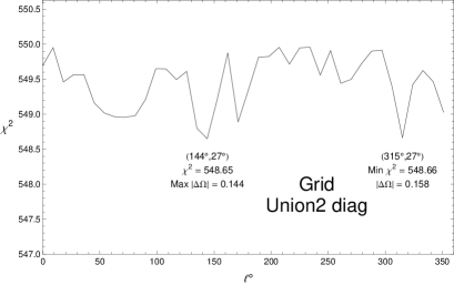
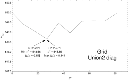
Figure 2: Real Union2 with diagonal-only errors: projection of $\chi^{2}$ vs galactic longitude (left) and latitude (right) from MCMC (top) and regular grid (bottom).

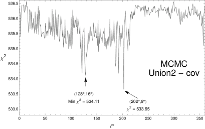
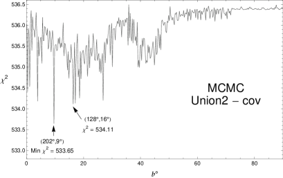
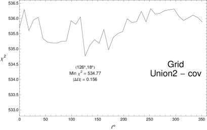
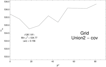
Figure 3: Real Union2 with total covariance matrix: projection of $\chi^{2}$ vs galactic longitude (left) and latitude (right) from MCMC (top) and regular grid (bottom).

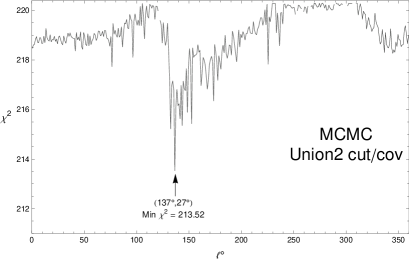
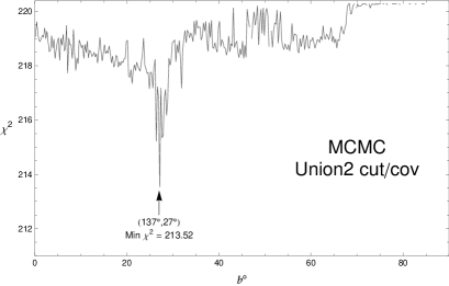
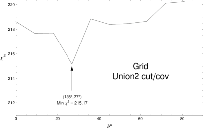
Figure 4: Real cut Union2 with diagonal-only errors: projection of $\chi^{2}$ vs galactic longitude (left) and latitude (right) from MCMC (top) and regular grid (bottom).

For each one of the previous cases, we have also performed an analysis similar to (Antoniou:2010gw, ): we have chosen $400$ directions, and found for the $\Omega^{N}_{m}$ and $\Omega^{S}_{m}$ values which minimize the $\chi^{2}$ function. As main differences with (Antoniou:2010gw, ) we have:

• built a regular grid of direction instead of choosing random directions. The coordinates have a grid step of $9$°  both in $l$ and $b$. It would certainly be more appropriate to build a grid such that all sky cells have the same area. However, we have chosen a step-size such that we do not expect big differences between both ways of building the grid;

• minimized the total $\chi^{2}$, instead of minimizing the north and south $\chi^{2}$ independently.

This has to be considered as a consistency test: by comparing MCMC results and the grid ones, we can test if and in what they differ, or not. Results are quite interesting and are shown in Figs. 2, 3 and 4. We should remind here the main difference between the two methods. When using the grid, we minimize the $\chi^{2}$ with respect to $\Omega^{N}_{m}$ and $\Omega^{S}_{m}$ for each direction and, consequently, in the corresponding figures we plot the best $\chi^{2}$ values for each chosen direction (i.e. fixing $\Omega^{N}_{m}$ and $\Omega^{S}_{m}$ at the found best fit values). On the contrary, the MCMC shows us the full angular dependence of the $\chi^{2}$ function, and the values in the figures could not correspond to the the best $\chi^{2}$ values for each depicted coordinates set. In some sense, the information from MCMC is more complete and detailed because we perform a full exploration of the spatial variation of the $\chi^{2}$.

V.1 Total sample cases

We can easily check by visual inspection, how MCMC reproduces at a very high accuracy the grid results, as a further confirmation of its goodness. With respect to the grid method, the MCMC have the improved feature of a complete span of the full parameter space. This feature eliminates the doubts about whether the number of grid/random directions is enough or not for the statistical analysis. In some cases we can also check one clear improvement from using MCMC: it finds some set of preferred parameters which cannot be analyzed by the grid method, neither with a regular grid or a random directions selection, as in (Antoniou:2010gw, ). Finally, it gives a direct and straightforward system to derive errors on all the parameters involved in the analysis, as they can be extracted directly from the MCMC outputs.

Concerning the case of diagonal-only errors, Fig. 2, we can see how the direction corresponding to the minimum of $\chi^{2}$ is slightly different from the one corresponding to the maximum anisotropy parameter $|\Delta\Omega_{m}|$: the former corresponding to the plane identified by coordinates $(144$°$,27$°$)$, the latter to $(315$°$,27$°$)$. This last direction is very close to the one identified in (Antoniou:2010gw, ) (differences arise only from the randomness versus regular grid choices we have used), but it is not statistically preferred, as its $\chi^{2}$ is not the best found. Thus, assuming this as the anisotropy axis is doubtful. Moreover, when moving to the total covariance error matrix, Fig. 3, we see how this direction now disappears, while a new one, namely $(202$°$,9$°$)$, is present. The MCMC confirms these directions, giving also a more complete sketch of the remaining parameter space.

The two cases, diagonal-only and full covariance matrix, also share a common property: in both of them, there is a direction which results to be associated with very low values of the $\chi^{2}$. It corresponds approximately to $l\approx(122$°$-128$°$)$ and $b\approx(16$°$-27$°$)$. These values might have to be considered with more attention because they correspond to the SDSS observational plane. We show it in Fig. 5: the plane described above is in red, while the SDSS SNeIa are shown as black points. The correspondence between the two is strikingly evident, and it is only slightly weakened when using the total covariance matrix for the higher error budget considered. If we think that the SDSS are approximately the $23\%$ of the total sample, and are highly clustered, they might be considered as an intrinsic strong bias in this analysis.

Finally, by looking at Table 1 and at the very close values of the $\chi^{2}$ shown in the Figs. 2 and 3, we can see that in the total diag and the total cov cases, no anisotropy is found, neither for what concerns its amount ($\Omega^{N}_{m}$ and $\Omega^{S}_{m}$ are perfectly consistent) nor for its direction (no preferred axis is found). This is not in conflict with results in (Antoniou:2010gw, ) if we consider that errors on $\Omega_{m}$ are approximately double when moving from a diagonal to a full covariance matrix. In (Antoniou:2010gw, ), using diagonal errors, it is argued that there is not a clear evidence for anisotropy. With a full covariance matrix we can here assess that no anisotropy is found at all.

Figure 5: This plot shows the distribution of SNIa from the Union2 compilation in the sky. The red circle and arrow represent respectively the anisotropy-equatorial plane and the orthogonal direction to such a plane with galactic coordinates $l_{a}=122$°  and $b_{a}=27$°  from the real diag Union2 analysis. Black points are SNIa from the SDSS sample; light gray points are SNIa from other sub-samples in the Union2 data set.

V.2 Cut sample cases

There seems to be a clear evidence that the statistical analysis using the full Union2 sample is dominated by the SDSS subset, aligned with SDSS scanning direction, and that such a subset is introducing a strong bias in the best fits. This is the reason for defining the cut sample, where SDSS and SNLS SNeIa are removed in order to have a more homogeneous distribution of supernovae. This might help to assess more clearly for a detected anisotropy, even though the cut in the number of data will inevitably degrade the signal (if any), as we have shown in the preliminary analysis with mock data.

Effectively, working with the cut sample and the full covariance matrix gives much more interesting hints (see last row of Table. 1). In that case we found an anisotropic signal in terms of both amount and direction. First, we wish to point out a quite clearly defined difference in the $\Omega_{m}$ values: the minimum in $\chi^{2}$ corresponds approximately to $\Omega_{m}^{N}\approx 0.25$ for the north pole, and $\Omega_{m}^{S}\approx 0.55$ for the south pole. Furthermore, we are also able to find an anisotropy direction, namely the orientation of the anisotropy-equatorial plane: $l_{a}=137$°  and $b_{a}=27$°. In Fig. 6 we show the $\chi^{2}$ full-sky distribution when a $\mathcal{N}=800$-cells grid is considered. Unfortunately, the low number of data left after the cut does not allow to give a high statistical significance to such a detection.

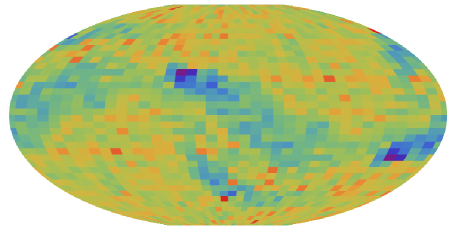
Figure 6: Full-sky $\Delta\chi^{2}$ map. A grid with $800$ cells is considered; the spacing is $18$°in $l_{a}$ (horizontal axis) and $2.25$°in $b_{a}$ (vertical axis). Blue corresponds to $\Delta\chi^{2}=0$; red to $\Delta\chi^{2}=25$.

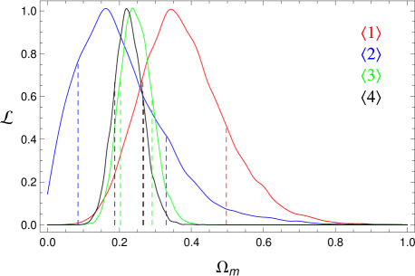
Figure 7: Here we show the likelihoods for $\Omega_{m}$ as obtained from the 4 different beams of the SNLS3 compilation. We observe no significant tension between them.

V.3 SNLS3 fits

Finally, we also consider the SNLS3 SNIa for our analysis. As we have discussed, their angular distribution can be seen as a paradigmatic badly suited sample for testing isotropy on full-sky ranges. But their interesting feature of being aligned along four directions makes them a specially suitable dataset to look for deviations with respect to isotropy in a scanning mode, in a way as the one suggested in Linder to be the optimal manner. However, we have to keep in mind that the number of SNIa in each beam is still quite low and a large error should be expected. In any case, this is a very interesting pattern that could be very useful for isotropy tests like the one performed here if a higher number of supernovae is detected along each direction in future observations.

We have applied a line-of-sight approach to this compilation of SNIa by independently fitting the supernovae of each beam searching for a possible direction-dependent change in $\Omega_{m}$. The results are shown in Fig. 7:. We do not find any significant deviation from isotropy, but only a small evidence for possibly different values of $\Omega_{m}$:

$$\Omega_{m}^{<1>} = 0.368^{+0.129}_{-0.103}$$

$$\Omega_{m}^{<2>} = 0.186^{+0.145}_{-0.101}$$

$$\Omega_{m}^{<3>} = 0.245^{+0.046}_{-0.042}$$

$$\Omega_{m}^{<4>} = 0.225^{+0.041}_{-0.038}$$

The likelihoods of two of the beams (3,4) peak at $\Omega_{m}$ values which are very similar to each other, but the peak values for the other two are quite disimilar: one is rather higher (1) and the other rather lower (2). However, the low number of SNIa ($\approx 60$ SNeIa in each beam) makes the likelihoods be sufficiently wide as to overlap at the $1\sigma$ level. But it is not to be discarded that in the future, with more SNeIa, one could perhaps be able to obtain stronger and more stringent constraints (or not).

VI Conclusions

In this work we have presented some new updated results when searching for an anisotropy signal using SNIa measurements. We have used the hemispherical comparison method consisting on fitting opposite hemispheres with independent $\Lambda$CDM models with the aim of finding an anisotropic distribution of $\Omega_{m}$. We have used the Union2 compilation throughout our analysis. Unlike some previous studies, we have considered the full covariance matrix for the SNIa errors and found that it plays a very important role. In fact, considering the full matrix introduces larger errors than those obtained when using only the diagonal errors. Thus, previously reported detections of anisotropy in SNIa observations go away completely when introducing the existing correlated errors. Moreover, we have used MCMC method, which implies a full detailed angular mapping of the $\chi^{2}$ function, allowing to discard possible false minima that could affect the grid or random orientations methods. Our result is in agreement with those in Heneka:2013hka , where no significant indication of hemispherical anisotropy was found. Moreover, we have shown that the particular alignment of the SDSS SNIa seems to introduce a strong bias when searching for anisotropic features. On the other hand, we have used the SNLS3 data and have taken advantage of its very special distribution with the SNIa lying along four different directions. We have then fitted each direction to an independent $\Lambda$CDM model and have obtained the corresponding matter density parameters. Although the four directions yield likelihoods overlapping at the $1\sigma$ level, we have found that two of the directions give likelihoods that peak at quite different values of $\Omega_{m}$. However, the low number of SNIa in each direction does not allow to draw any significant conclusion.

Acknowledgements J.B.J. is supported by the Wallonia-Brussels Federation grant ARC No. 11/15-040 and also thanks support from the Spanish MICINN Consolider-Ingenio 2010 Programme under grant MultiDark CSD2009-00064 and project number FIS2011-23000. J.B.J. also wishes to acknowledges the Department of Theoretical physics of the University of the Basque Country for their warm hospitality. V.S. and R.L. are supported by the Spanish Ministry of Economy and Competitiveness through research projects FIS2010-15492 and Consolider EPI CSD2010-00064, and also by the Basque Government through research project GIC12/66, and by the University of the Basque Country UPV/EHU under program UFI 11/55.

References

- (1) P. A. R. Ade, N. Aghanim, C. Armitage-Caplan, et al., 2013 [arXiv:1303.5076]
- (2) S. M. Carroll, W. H. Press, E. L. Turner, ARA&A (1992) 30 499; V. Sahni, A. Starobinski, Int. J. Mod. Phys. D (2000) 9 373.
- (3) S. Weinberg, Cosmology (Oxford University Press, New York, New York, 2008).
- (4) L. Perivolaropoulos, 2011 [arXiv:1104.0539]; L. Perivolaropoulos, 2008 [arXiv:0811.4684]; R. J. Yang, S. N. Zhang, MNRAS (2010) 407 1835.
- (5) L. Campanelli, P. Cea and L. Tedesco, Phys. Rev. Lett. 97 (2006) 131302 [Erratum-ibid. 97 (2006) 209903] [astro-ph/0606266].
- (6) A. L. Maroto, JCAP 0605 (2006) 015 [astro-ph/0512464]. A. L. Maroto, Int. J. Mod. Phys. D 15 (2006) 2165 [astro-ph/0605381]. A. L. Maroto, AIP Conf. Proc. 878 (2006) 240 [astro-ph/0609218].
- (7) J. Beltran Jimenez and A. L. Maroto, Phys. Rev. D 76 (2007) 023003 [astro-ph/0703483].
- (8) J. Beltran Jimenez and A. L. Maroto, JCAP 0903 (2009) 015 [arXiv:0811.3606 [astro-ph]].
- (9) T. Harko and F. S. N. Lobo, JCAP 1307 (2013) 036 [arXiv:1304.0757 [gr-qc]].
- (10) D. C. Rodrigues, Phys. Rev. D 77 (2008) 023534 [arXiv:0708.1168 [astro-ph]].
- (11) T. Koivisto and D. F. Mota, Astrophys. J. 679 (2008) 1 [arXiv:0707.0279 [astro-ph]]. T. Koivisto and D. F. Mota, JCAP 0806 (2008) 018 [arXiv:0801.3676 [astro-ph]].
- (12) R. A. Battye and A. Moss, Phys. Rev. D 74 (2006) 041301 [astro-ph/0602377]. R. A. Battye and A. Moss, Phys. Rev. D 76 (2007) 023005 [astro-ph/0703744 [ASTRO-PH]].
- (13) L. Campanelli, P. Cea, G. L. Fogli and L. Tedesco, Int. J. Mod. Phys. D 20 (2011) 1153 [arXiv:1103.2658 [astro-ph.CO]].
- (14) S. A. Appleby, E. V. Linder, Phys. Rev. D (2013) 87 023532.
- (15) T. S. Koivisto, D. F. Mota, M. Quartin and T. G. Zlosnik, Phys. Rev. D 83 (2011) 023509 [arXiv:1006.3321 [astro-ph.CO]].
- (16) S. Appleby, R. Battye and A. Moss, Phys. Rev. D 81 (2010) 081301 [arXiv:0912.0397 [astro-ph.CO]].
- (17) T. S. Kolatt and O. Lahav, Mon. Not. Roy. Astron. Soc. 323 (2001) 859 [astro-ph/0008041].
- (18) C. Bonvin, R. Durrer and M. Kunz, Phys. Rev. Lett. 96 (2006) 191302 [astro-ph/0603240].
- (19) C. Bonvin, R. Durrer and M. A. Gasparini, Phys. Rev. D 73 (2006) 023523 [Erratum-ibid. D 85 (2012) 029901] [astro-ph/0511183]. E. Di Dio and R. Durrer, Phys. Rev. D 86 (2012) 023510 [arXiv:1205.3366 [astro-ph.CO]].
- (20) D. J. Schwarz and B. Weinhorst, Astron. Astrophys. 474 (2007) 717 [arXiv:0706.0165 [astro-ph]]. J. Colin, R. Mohayaee, S. Sarkar and A. Shafieloo, Mon. Not. Roy. Astron. Soc. 414 (2011) 264 [arXiv:1011.6292 [astro-ph.CO]]. B. Kalus, D. J. Schwarz, M. Seikel and A. Wiegand, Astron. Astrophys. 553 (2013) A56 [arXiv:1212.3691 [astro-ph.CO]].
- (21) U. Feindt, M. Kerschhaggl, M. Kowalski, G. Aldering, P. Antilogus, C. Aragon, S. Bailey and C. Baltay et al., Astron. Astrophys. (2013) [arXiv:1310.4184 [astro-ph.CO]]. B. Rathaus, E. D. Kovetz and N. Itzhaki, arXiv:1301.7710 [astro-ph.CO].
- (22) I. Antoniou and L. Perivolaropoulos, JCAP 1012 (2010) 012.
- (23) R. -G. Cai and Z. -L. Tuo, JCAP 1202 (2012) 004 [arXiv:1109.0941 [astro-ph.CO]].
- (24) M. Blomqvist, J. Enander and E. Mortsell, JCAP 1010 (2010) 018 [arXiv:1006.4638 [astro-ph.CO]].
- (25) A. Mariano and L. Perivolaropoulos, Phys. Rev. D 86 (2012) 083517 [arXiv:1206.4055 [astro-ph.CO]].
- (26) R. -G. Cai, Y. -Z. Ma, B. Tang and Z. -L. Tuo, Phys. Rev. D 87 (2013) 123522 [arXiv:1303.0961 [astro-ph.CO]].
- (27) L. Amendola, V. Marra and M. Quartin, Mon. Not. Roy. Astron. Soc. 430 (2013) 1867 [arXiv:1209.1897 [astro-ph.CO]].
- (28) C. Heneka, V. Marra and L. Amendola, arXiv:1310.8435 [astro-ph.CO].
- (29) J. Guy, M. Sullivan, A. Conley, et al., Astron. Astrophys. 523 (2010) 7; A. Conley, J. Guy, M. Sullivan, et al., Astrophys. J. Supp. 192 (2011) 1; M. Sullivan, J. Guy, A. Conley, et al., Astrophys. J. 737 (2011)102S.
- (30) J. A. Frieman, B. Bassett, A. Becker, et al., The Astronomical Journal 135 (2008) 338; M. Sako, B. Bassett, A. Becker, et al., The Astronomical Journal 135 (2008) 348; J. A. Holtzmann, J. Marriner, R. Kessler, et al., The Astronomical Journal 136 (2008) 2306.
- (31) R. Amanullah, C. Lidman, D. Rubin, et al., ApJ 716 (2010) 712; N. Suzuki, D. Rubin, C. Lidman, et al., ApJ 746 (2012) 85;
- (32) A. Rest, D. Scolnic, R. J. Foley, M. E. Huber, R. Chornock, G. Narayan, J. L. Tonry and E. Berger et al., arXiv:1310.3828 [astro-ph.CO].
- (33) H. K. Eriksen, F. K. Hansen, A. J. Banday, K. M. Gorski and P. B. Lilje, Astrophys. J. 605 (2004) 14 [Erratum-ibid. 609 (2004) 1198].
- (34) Dunkley, J., Bucher, M., Ferreira, P.G., Moodley, K., Skordis, C., 2005, Mon. Not. R. Astron. Soc. 356, 925.