Abstract

We focus on the distribution regression problem: regressing to a real-valued response from a probability distribution. Although there exist a large number of similarity measures between distributions, very little is known about their generalization performance in specific learning tasks. Learning problems formulated on distributions have an inherent two-stage sampled difficulty: in practice only samples from sampled distributions are observable, and one has to build an estimate on similarities computed between sets of points. To the best of our knowledge, the only existing method with consistency guarantees for distribution regression requires kernel density estimation as an intermediate step (which suffers from slow convergence issues in high dimensions), and the domain of the distributions to be compact Euclidean. In this paper, we provide theoretical guarantees for a remarkably simple algorithmic alternative to solve the distribution regression problem: embed the distributions to a reproducing kernel Hilbert space, and learn a ridge regressor from the embeddings to the outputs. Our main contribution is to prove the consistency of this technique in the two-stage sampled setting under mild conditions (on separable, topological domains endowed with kernels). For a given total number of observations, we derive convergence rates as an explicit function of the problem difficulty. As a special case, we answer a $15$-year-old open question: we establish the consistency of the classical set kernel [Haussler, 1999; Gärtner et. al, 2002] in regression, and cover more recent kernels on distributions, including those due to [Christmann and Steinwart, 2010].

1 INTRODUCTION

We address the learning problem of distribution regression in the two-stage sampled setting [1]: we regress from probability measures to real-valued responses, where we only have bags of samples from the probability distributions. Many classical problems in machine learning and statistics can be analysed in this framework. On the machine learning side, multiple instance learning [2, 3, 4] can be thought of in this way, in the case where each instance in a labeled bag is an i.i.d. (independent identically distributed) sample from a distribution. On the statistical side, tasks might include point estimation of statistics on a distribution (e.g., its entropy or a hyperparameter), where a supervised learning method can help in parameter estimation problems without closed form analytical expressions, or if simulation-based results are computationally expensive.

Before reviewing the existing techniques in the literature, let us start with a somewhat informal definition of the distribution regression problem, and an intuitive phrasing of our goal. Let us suppose that our data consist of $\mathbf{z}=\{(x_{i},y_{i})\}_{i=1}^{l}$, where $x_{i}$ is a probability distribution, $y_{i}\in\mathbb{R}$, and each $(x_{i},y_{i})$ pair is i.i.d. sampled from a meta distribution $\mathcal{M}$. However, we do not observe $x_{i}$ directly; rather, we observe a sample $x_{i,1},\ldots,x_{i,N_{i}}\stackrel{{\scriptstyle i.i.d.}}{{\sim}}x_{i}$. Thus the observed data are $\hat{\mathbf{z}}=\{(\{x_{i,n}\}_{n=1}^{N_{i}},y_{i})\}_{i=1}^{l}$. Our goal is to predict a new $y_{l+1}$ from a new batch of samples $x_{l+1,1},\ldots,x_{l+1,N_{l+1}}$ drawn from a new distribution $x_{l+1}$. For example, in a medical application the $i^{th}$ patient might be identified with a probability distribution ($x_{i}$), which can be periodicly accessed, measured by blood tests ($\{x_{i,n}\}_{n=1}^{N_{i}}$). We are also given some health indicator of the patient ($y_{i}$), which might be inferred from his/her blood measurements. Based on the observations ($\hat{\mathbf{z}}$), one might try to learn the mapping from the set of blood tests to the health indicator; and the hope is that by observing more patients (larger $l$) and performing a larger number of tests (larger $N_{i}$) the estimated mapping ($\hat{f}=\hat{f}({\hat{\mathbf{z}}})$) becomes more “precise”.

The performance of the estimated mapping ($\hat{f}$) depends on the assumed function class ($\mathscr{H}$), the family of $\hat{f}$ candidates. Let $f_{\mathscr{H}}$ denote the best estimator from $\mathscr{H}$ given infinite training samples ($l=\infty$, $N_{i}=\infty$), and let $\mathcal{E}[f_{\mathscr{H}}]$ be its prediction error. Our goal is to obtain upper bounds for the $0\leq\mathcal{E}[\hat{f}]-\mathcal{E}[f_{\mathscr{H}}]$ quantity which hold with high probability. More precisely, we are aiming at

1. deriving upper bounds on the excess risk, proving consistency: We construct $\mathcal{E}[\hat{f}]-\mathcal{E}[f_{\mathscr{H}}]\leq r(l,N,\lambda)$ bounds, where $\lambda$ is a regularization parameter converging to zero as we see more samples ($l\rightarrow\infty$, $N=N_{i}\rightarrow\infty$), and choose the $(l,N,\lambda)$ triplet appropriately to drive $r(l,N,\lambda)$ and hence $\mathcal{E}[\hat{f}]-\mathcal{E}[f_{\mathscr{H}}]$ to $0$.

2. obtaining convergence rates: We establish convergence rates for a general prior family $\mathcal{P}(b,c)$ [5], where $b$ captures the effective input dimension, and larger $c$ means smoother $f_{\mathscr{H}}$. In particular, when $l=N^{a}$ ($a>0$), the effective dimension is small (large $b$), and the total number of samples processed $t=lN=N^{a+1}$ is fixed, one obtains a rate of $1/t^{2/7}$ for a smooth regression function ($c=2$), $1/t^{1/5}$ in the non-smooth case ($c=1$).

The motivation for considering the $\mathcal{P}(b,c)$ family is two-fold:

1. it does not assume parametric distributions, still certain complexity terms can be explicitly upper bounded in the family. This property will be exploited in our analysis.

2. (for special input distributions) parameter $b$ can be related to the spectral decay of Gaussian Gram matrices, thus available analysis techniques [6] might give alternative prior characterizations.

Briefly, we focus on the following question:

Can the distribution regression problem be solved consistently under mild conditions?

Despite the large number of available “solutions” and applications of distribution regression dating back to $1999$ [7], surprisingly this pretty fundamental question has hardly been touched. In our paper we give affirmative answer to the question by presenting the analysis of a simple kernel ridge regression approach [see Eq. (3)] in the two-stage sampled ($\mathscr{M}\rightarrow\mathbf{z}\rightarrow\hat{\mathbf{z}}$) setting.

Review of approaches to learning on distributions: A number of methods have been proposed over the years to compute the similarity of distributions or bags of samples. As a first approach, one could fit a parametric model to the bags, and estimate the similarity of the bags based on the obtained parameters. It is then possible to define learning algorithms on the basis of these similarities, which often take analytical form. Typical examples with explicit formulas include Gaussians, finite mixtures of Gaussians, and distributions from the exponential family (with known log-normalizer function and zero carrier measure) [8, 9, 10, 11]. A major limitation of these methods, however, is that they apply quite simple parametric assumptions, which may not be sufficient or verifiable in practise.

A heuristic related to the parametric approach is to assume that the training distributions are Gaussians in a reproducing kernel Hilbert space; see for example [10, 12] and references therein. This assumption is algorithmically appealing, as many divergence measures for Gaussians can be computed in closed form using only inner products, making them straightforward to kernelize. A fundamental shortfall of kernelized Gaussian divergences is the lack of their consistency analysis in specific learning algorithms.

A more theoretically grounded approach to learning on distributions has been to define positive definite kernels [13] on the basis of statistical divergence measures on distributions, or by metrics on non-negative numbers; these can then be used in kernel algorithms. This category includes work on semigroup kernels [14], nonextensive information theoretical kernel constructions [15], and kernels based on Hilbertian metrics [16]. For example, in [14] the intuition is as follows: if two measures or sets of points overlap, then their sum is expected to be more concentrated. The value of dispersion can be measured by entropy or inverse generalized variance. In the second type of approach [16], homogeneous Hilbert metrics on the non-negative real line are used to define the similarity of probability distributions. While these techniques guarantee to provide valid kernels on certain restricted domains of measures, the performance of learning algorithms based on finite sample estimates of these kernels remains a challenging open question. One might also plug into learning algorithms (based on similarities of distributions) consistent Rényi and Tsallis divergence estimates [17, 18], but these similarity indices are not kernels, and their consistency in specific learning tasks, similarly to the previous works, is open.

To the best of our knowledge, the only prior work addressing the consistency of regression on distributions requires kernel density estimation [1, 19], assumes that the response variable is scalar-valued, and the covariates are nonparametric continuous distributions on $\mathbb{R}^{d}$. As in our setting, the exact forms of these distributions are unknown; they are available only through finite sample sets. Póczos et al. estimated these distributions through a kernel density estimator (assuming these distributions to have a density) and then constructed a kernel regressor that acts on these kernel density estimates. Using the classical bias-variance decomposition analysis for kernel regressors, they show the consistency of the constructed kernel regressor, and provide a polynomial upper bound on the rates, assuming the true regressor to be Hölder continuous, and the meta distribution that generates the covariates $x_{i}$ to have finite doubling dimension [22].

An alternative paradigm in learning when the inputs are “bags of objects” is to simply treat each input as a finite set, and to define kernel learning algorithms based on set kernels [23] (also called multi-instance kernels or ensemble kernels, and instances of convolution kernels [7]). In this case, the similarity of two sets is measured by the average pairwise point similarities between the sets. From a theoretical perspective, very little has been done to establish the consistency of set kernels in learning since their introduction in 1999 [7, 23]: i.e. in what sense (and with what rates) is the learning algorithm consistent, when the number of items per bag, and the number of bags, is allowed to increase?

It is possible, however, to view set kernels in a distribution setting, as they represent valid kernels between (mean) embeddings of empirical probability measures into a reproducing kernel Hilbert space (RKHS) [24]. The population limits are well-defined as being dot products between the embeddings of the generating distributions [25], and for characteristic kernels the distance between embeddings defines a metric on probability measures [26, 27]. When bounded kernels are used, mean embeddings exist for all probability measures [28]. When we consider the distribution regression setting, however, there is no reason to limit ourselves to set kernels. Embeddings of probability measures to RKHS are used by [29] in defining a yet larger class of easily computable kernels on distributions, via operations performed on the embeddings and their distances. Note that the relation between set kernels and kernels on distributions has been applied by [30] for classification on distribution-valued inputs, however consistency was not studied in that work.

Our contribution in this paper is to establish the consistency of an algorithmically simple, mean embedding based ridge regression method (described in Section 2) for the distribution regression problem. This result applies both to the basic set kernels of [7, 23], the distribution kernels of [29], and additional related kernels proposed herein. We provide two-stage sampled excess error bounds, consistency proof and convergence rates in Section 4, and break down the various tradeoffs arising in different sample size and problem difficulties. The principal challenge in proving theoretical guarantees arises from the two-stage sampled nature of the inputs. In our analysis, we make use of [5], who provide error bounds for the one-stage sample setup. These results will make our analysis somewhat shorter (but still rather challenging) by giving upper bounds for some of the upcoming objective terms. Even the verification of these conditions requires care (Section 3) since the inputs in the ridge regression are themselves distribution embeddings (i.e., functions in a reproducing kernel Hilbert space).

Due to the differences in the assumptions made and the loss function used, a direct comparison of our theoretical result and that of [1]³ remains an open question, however we make two observations. First, our approach is more general, since we may regress from any probability measure defined on a separable, topological domain endowed with a kernel. Póczos et al.’s work is restricted to compact domains of finite dimensional Euclidean spaces, and requires the distributions to admit probability densities; distributions on strings, time series, graphs, and other structured objects are disallowed. Second, density estimates in high dimensional spaces suffer from slow convergence rates [31, Section 6.5]. Our approach avoids this problem, as it works directly on distribution embeddings, and does not make use of density estimation as an intermediate step.

2 THE DISTRIBUTION REGRESSION PROBLEM

In this section, we define the distribution regression problem, for a general RKHS on distributions. In Section 3, we will provide examples of valid kernels for this RKHS, including set kernels [7, 23], the kernels from [29], and further related kernels. Below, we first introduce some notation and then formally discuss the distribution regression problem.

Notation: Let $(\mathscr{X},\tau)$ be a topological space and let $\mathcal{B}(\mathscr{X}):=\mathcal{B}(\tau)$ be the Borel $\sigma$-algebra induced by the topology $\tau$. $\mathscr{M}_{1}^{+}(\mathscr{X})$ denotes the set of Borel probability measures on $(\mathscr{X},\mathcal{B}(\mathscr{X}))$. The weak topology ($\tau_{w}=\tau_{w}(\mathscr{X},\tau)$) on $\mathscr{M}^{+}_{1}(\mathscr{X})$ is defined as the weakest topology such that the $L_{h}:(\mathscr{M}^{+}_{1}(\mathscr{X}),\tau_{w})\rightarrow\mathbb{R}$, $L_{h}(x)=\int_{\mathscr{X}}h(u)\mathrm{d}x(u)$ mapping is continuous for all $h\in C_{b}(\mathscr{X})=\{(\mathscr{X},\tau)\rightarrow\mathbb{R}\text{ bounded, continuous functions}\}$. Let $H=H(k)$ be the RKHS [6] with $k:\mathscr{X}\times\mathscr{X}\rightarrow\mathbb{R}$ as the reproducing kernel. Denote by

$$X =\mu\left(\mathscr{M}^{+}_{1}\left(\mathscr{X}\right)\right)=\{\mu_{x}:x\in\mathscr{M}^{+}_{1}\left(\mathscr{X}\right)\}\subseteq H$$

the set of $\mu_{x}=\int_{\mathscr{X}}k(\cdot,u)\mathrm{d}x(u)=\mathbb{E}_{u\sim x}[k(\cdot,u)]\in H$ mean embeddings [24] of the distributions to the space $H$, and let $Y=\mathbb{R}$. Intuitively, $\mu_{x}$ is the canonical feature map [$k(\cdot,u)$] averaged according to the probability measure [$\mathrm{d}x(u)$]. Let $\mathscr{H}=\mathscr{H}(K)$ be the RKHS of functions with $K:X\times X\rightarrow\mathbb{R}$ as the reproducing kernel. $\mathscr{L}(\mathscr{H})$ is the space of $\mathscr{H}\rightarrow\mathscr{H}$ bounded linear operators, and $\delta_{\mu_{a}}$ denotes the evaluation functional at $\mu_{a}$ ($a\in\mathscr{M}^{+}_{1}(\mathscr{X})$). For $M\in\mathscr{L}(\mathscr{H})$ the operator norm is defined as $\left\|M\right\|_{\mathscr{L}(\mathscr{H})}=\sup_{0\neq q\in\mathscr{H}}\frac{\left\|Mq\right\|_{\mathscr{H}}}{\left\|q\right\|_{\mathscr{H}}}$. Given $(U_{1},\mathscr{S}_{1})$ and $(U_{2},\mathscr{S}_{2})$ measurable spaces the $\mathscr{S}_{1}\otimes\mathscr{S}_{2}$ product $\sigma$-algebra [6, page 480] on the product space $U_{1}\times U_{2}$ is the $\sigma$-algebra generated by the cylinder sets $U_{1}\times S_{2}$, $S_{1}\times U_{2}$ ($S_{1}\in\mathscr{S}_{1}$, $S_{2}\in\mathscr{S}_{2}$). $\mathbb{E}[\cdot]$ denotes expectation.

Distribution regression: In the distribution regression problem, we are given samples $\hat{\mathbf{z}}=\{(\{x_{i,n}\}_{n=1}^{N_{i}},y_{i})\}_{i=1}^{l}$ with $x_{i,1},\ldots,x_{i,N_{i}}\stackrel{{\scriptstyle i.i.d.}}{{\sim}}x_{i}$ where $\mathbf{z}=\{(x_{i},y_{i})\}_{i=1}^{l}$ with $x_{i}\in\mathscr{M}^{+}_{1}\left(\mathscr{X}\right)$ and $y_{i}\in Y$ drawn i.i.d. from a joint meta distribution $\mathcal{M}$ defined on the measurable space $(\mathscr{M}^{+}_{1}(\mathscr{X})\times\mathbb{R},\mathcal{B}(\tau_{w})\otimes\mathcal{B}(\mathbb{R}))$. Unlike in classical supervised learning problems, the problem at hand involves two levels of randomness, wherein first $\mathbf{z}$ is drawn from $\mathcal{M}$ and then $\hat{\mathbf{z}}$ is generated by sampling points from $x_{i}$ for all $i=1,\ldots,l$. The goal is to learn the relation between the random distribution $x$ and scalar response $y$ based on the observed $\hat{\mathbf{z}}$. For notational simplicity, we will assume that $N=N_{i}$ ($\forall i$).

As in the classical regression task ($\mathbb{R}^{d}\rightarrow\mathbb{R}$), distribution regression can be tackled as a kernel ridge regression problem (using squared loss as the discrepancy criterion). The kernel (say $k_{\mathscr{G}}$) is defined on $\mathscr{M}^{+}_{1}(\mathscr{X})$, and the regressor is then modelled by an element in the RKHS $\mathscr{G}=\mathscr{G}(k_{\mathscr{G}})$ of functions mapping from $\mathscr{M}^{+}_{1}(\mathscr{X})$ to $\mathbb{R}$. In this paper, we choose $k_{\mathscr{G}}(x,x^{\prime})=K(\mu_{x},\mu_{x^{\prime}})$ where $x,x^{\prime}\in\mathscr{M}^{+}_{1}(\mathscr{X})$ and so that the function (in $\mathscr{G}$) to describe the $(x,y)$ random relation is constructed as a composition

$$\mathscr{M}^{+}_{1}\left(\mathscr{X}\right)\xrightarrow{\mu}X(\subseteq H=H(k))\xrightarrow{f\in\mathscr{H}=\mathscr{H}(K)}\mathbb{R}.$$

In other words, the distribution $x\in\mathscr{M}^{+}_{1}\left(\mathscr{X}\right)$ is first mapped to $X\subseteq H$ by the mean embedding $\mu$, and the result is composed with $f$, an element of the RKHS $\mathscr{H}=\mathscr{H}(K)$. Assuming that $f_{\mathscr{G}}$, the minimizer of the expected risk ($\mathcal{E}$) over $\mathscr{G}$ exists, then a function $f_{\mathscr{H}}$ also exists, and satisfies

$$\mathcal{E}\left[f_{\mathscr{H}}\right] =\inf_{f\in\mathscr{H}}\mathcal{E}[f]=\inf_{f\in\mathscr{H}}\mathbb{E}_{(x,y)\sim\mathcal{M}}[f(\mu_{x})-y]^{2}$$

$$=\inf_{g\in\mathscr{G}}\mathbb{E}_{(x,y)\sim\mathcal{M}}[g(x)-y]^{2}=\inf_{g\in\mathscr{G}}\mathcal{E}[g]=\mathcal{E}\left[g_{\mathscr{G}}\right].$$

The classical regularization approach is to optimize

$$f_{\mathbf{z}}^{\lambda} =\operatorname*{arg\,min}_{f\in\mathscr{H}}\frac{1}{l}\sum_{i=1}^{l}\left[f(\mu_{x_{i}})-y_{i}\right]^{2}+\lambda\left\|f\right\|_{\mathscr{H}}^{2}$$ (1)

instead of $\mathcal{E}$, based on samples $\mathbf{z}$. Since $\mathbf{z}$ is not accessible, we consider the objective function defined by the observable quantity $\hat{\mathbf{z}}$,

$$f_{\hat{\mathbf{z}}}^{\lambda} =\operatorname*{arg\,min}_{f\in\mathscr{H}}\frac{1}{l}\sum_{i=1}^{l}\left[f(\mu_{\hat{x}_{i}})-y_{i}\right]^{2}+\lambda\left\|f\right\|_{\mathscr{H}}^{2},$$ (2)

where $\hat{x}_{i}=\frac{1}{N}\sum_{n=1}^{N}\delta_{x_{i,n}}$ is the empirical distribution determined by $\left\{x_{i,n}\right\}_{i=1}^{N}$. Algorithmically, ridge regression is quite simple [32]: given training samples $\hat{\mathbf{z}}$, the prediction for a new $t$ test distribution is

$$(f_{\hat{\mathbf{z}}}^{\lambda}\circ\mu)(t) =[y_{1},\ldots,y_{l}](\mathbf{K}+l\lambda\mathbf{I}_{l})^{-1}\mathbf{k}\in\mathbb{R},$$ (3)

$$\mathbf{K} =[K(\mu_{\hat{x}_{i}},\mu_{\hat{x}_{j}})]\in\mathbb{R}^{l\times l},$$

$$\mathbf{k} =\left[K(\mu_{\hat{x}_{1}},\mu_{t});\ldots;K(\mu_{\hat{x}_{l}},\mu_{t})\right]\in\mathbb{R}^{l}.$$

Remarks:

1. It is important to note that the algorithm has access to the sample points only via their mean embeddings $\{\mu_{\hat{x}_{i}}\}_{i=1}^{l}$ in Eq. (2).

2. There is a two-stage sampling difficulty to tackle: The transition from $f_{\mathscr{H}}$ to $f_{\mathbf{z}}^{\lambda}$ represents the fact that we have only $l$ distribution samples ($\mathbf{z}$); the transition from $f_{\mathbf{z}}^{\lambda}$ to $f_{\hat{\mathbf{z}}}^{\lambda}$ means that the $x_{i}$ distributions can be accessed only via samples ($\hat{\mathbf{z}}$).

3. While ridge regression can be performed using the kernel $k_{\mathscr{G}}$, the two-stage sampling makes it difficult to work with arbitrary $k_{\mathscr{G}}$. By contrast, our choice of $k_{\mathscr{G}}(x,x^{\prime})=K(\mu_{x},\mu_{x^{\prime}})$ enables us to handle the two-stage sampling by estimating $\mu_{x}$ with an empirical estimator and using it in the algorithm as shown above.

The main goal of this paper is to analyse the excess risk $\mathcal{E}[f_{\hat{\mathbf{z}}}^{\lambda}]-\mathcal{E}[f_{\mathscr{H}}]$, i.e., the regression performance compared to the best possible estimation from $\mathscr{H}$, and to establish consistency and rates of convergence as a function of the $(l,N,\lambda)$ triplet, and of the difficulty of the problem in the sense of [5].

3 ASSUMPTIONS

In this section we detail our assumptions on the $(\mathscr{X},k,K)$ triplet, and show that regressing with set kernels fit into the studied problem family. Our analysis will rely on existing ridge regression results [5] which focus on problem (1), where only a single-stage sampling is present; hence we have to verify the associated conditions. Though we make use of these results, the analysis still remains rather challenging; the available bounds can moderately shorten our proof. We must also take particular care in verifying that [5]’s conditions are met, since they must hold for the space of mean embeddings of the distributions ($X=\mu\left(\mathscr{M}_{1}^{+}(\mathscr{X})\right)$), whose properties as a function of $\mathscr{X}$ and $H$ must themselves be established. Our assumptions:

• $\exists f_{\mathscr{H}}$ such that $\mathcal{E}[f_{\mathscr{H}}]=\inf_{f\in\mathscr{H}}\mathcal{E}(f)$.

• $(\mathscr{X},\tau)$ is a separable, topological domain.

• $k:\mathscr{X}\times\mathscr{X}\rightarrow\mathbb{R}$ is bounded ($\exists B_{k}<\infty$ such that $\sup_{u\in\mathscr{X}}k(u,u)\leq B_{k}$) and continuous.

• $K:X\times X\rightarrow\mathbb{R}$ is bounded, i.e., $\exists B_{K}<\infty$ such that

  $$K(\mu_{a},\mu_{a}) \leq B_{K},\quad(\forall\mu_{a}\in X),$$ (4)

  and $\Psi(\mu_{c}):=K(\cdot,\mu_{c}):X\rightarrow\mathscr{H}$ is Hölder continuous, i.e., $\exists L>0$, $h\in(0,1]$ such that for $\forall(\mu_{a},\mu_{b})\in X\times X$

  $$\left\|\Psi(\mu_{a})-\Psi(\mu_{b})\right\|_{\mathscr{H}} \leq L\left\|\mu_{a}-\mu_{b}\right\|_{H}^{h}.$$ (5)

• $y$ is bounded: $\exists C<\infty$ such that $|y|\leq C$ almost surely.

• $X=\mu(\mathscr{M}^{+}_{1}(\mathscr{X}))\in\mathcal{B}(H)$.

Discussion of the assumptions: We give a short insight into the consequences of our assumptions and present some concrete examples.

1. The boundedness and continuity of $k$ imply the measurability of $\mu:(\mathscr{M}^{+}_{1}(\mathscr{X}),\mathcal{B}(\tau_{w}))\rightarrow(H,\mathcal{B}(H))$, which using the $X\in\mathcal{B}(H)$ condition guarantees that the $\rho$, the measure induced by $\mathscr{M}$ on $X\times\mathbb{R}$ is well-defined (see the supplementary material).

2. For a linear kernel, $K(\mu_{a},\mu_{b})=\left<\mu_{a},\mu_{b}\right>_{H}$, $(\mu_{a},\mu_{b}\in X)$, one can verify (see the supplementary material) that Hölder continuity holds with $L=1$, $h=1$. Also, since $K(\mu_{a},\mu_{b})\leq B_{k}$ for any $a,b\in\mathscr{M}^{+}_{1}(\mathscr{X})$, we can choose $B_{K}=B_{k}$. Evaluating the kernel, $K$ at the $\mu_{\hat{x}_{i}}=\int_{\mathscr{X}}k(\cdot,u)\mathrm{d}\hat{x}_{i}(u)=\frac{1}{N}\sum_{n=1}^{N}k(\cdot,x_{i,n})$ empirical embeddings yields the standard set kernel:

   $$K(\mu_{\hat{x}_{i}},\mu_{\hat{x}_{j}}) =\frac{1}{N^{2}}\sum_{n,m=1}^{N}k(x_{i,n},x_{j,m}).$$

3. One can also prove (see the supplement) by using the properties of negative/positive definite functions [33] that many $K$ functions on $X\times X$ are kernels and (in case of compact metric $\mathscr{X}$ domains) Hölder continuous. Some examples are listed in Table 1; these kernels are the natural extensions to distributions of the Gaussian [29], exponential, Cauchy, generalized t-student and inverse multiquadratic kernels.

4. $Y=\mathbb{R}$ is a separable Hilbert space hence Polish, and thus the $\rho(y|\mu_{a})$ conditional distribution ($y\in\mathbb{R}$, $\mu_{a}\in X$) is well-defined; see [6, Lemma A.3.16, page 487].

5. The separability of $\mathscr{X}$ and the continuity of $k$ implies the separability of $H$ [6, Lemma 4.33, page 130]. Also, since $X\subseteq H$, $X$ is separable; hence so is $\mathscr{H}$ due to the continuity of $K$.

Verification of [5]’s conditions: Below we prove that [5]’s conditions hold under our assumptions.

1. $Y=\mathbb{R}$ and $\mathscr{H}$ are separable Hilbert spaces – as we have seen.

2. By the bilinearity of $\left<\cdot,\cdot\right>_{\mathscr{H}}$ and the reproducing property of $K$, the measurability of $(\mu_{x},\mu_{t})\mapsto\left<K(\cdot,\mu_{x})w,K(\cdot,\mu_{t})v\right>_{\mathscr{H}}=wK(\mu_{x},\mu_{t})v\quad(\forall w,v\in\mathbb{R})$ is equivalent to that of $(\mu_{x},\mu_{t})\mapsto K(\mu_{x},\mu_{t})$; the latter follows from the Hölder continuity of $\Psi$ (see the supplement).

3. Due to the boundedness of $y$, we have $\int_{X\times\mathbb{R}}y^{2}\mathrm{d}\rho(\mu_{x},y)\leq\int_{X\times\mathbb{R}}C^{2}\mathrm{d}\rho(\mu_{x},y)\leq C^{2}<\infty$, and $\exists\Sigma>0,\exists M>0$ such that

   $$\int_{\mathbb{R}}e^{\frac{\left|y-f_{\mathscr{H}}(\mu_{x})\right|}{M}}-\frac{\left|y-f_{\mathscr{H}}(\mu_{x})\right|}{M}-1\mathrm{d}\rho(y|\mu_{x}) \leq\frac{\Sigma^{2}}{2M^{2}}$$ (6)

   for $\rho_{X}\text{-almost }\mu_{x}\in X$, where $\rho(\mu_{x},y)=\rho(y|\mu_{x})\rho_{X}(\mu_{x})$ is factorized into conditional and marginal distributions. (6) is a model of the noise of the output $y$; it is satisfied, for example in case of bounded noise [5, page 9]. By the boundedness of $y$ and that of kernel $K$ this property holds: $|y-f_{\mathscr{H}}(\mu_{x})|\leq|y|+|f_{\mathscr{H}}(\mu_{x})|\leq C+\left\|f_{\mathscr{H}}\right\|_{H}\sqrt{B_{K}}$, where we used the triangle inequality and Lemma 4.23 (page 124) from [6].

Table 1: Nonlinear kernels on mean embedded distributions: $K=K(\mu_{a},\mu_{b})$; $\theta>0$. For the Hölder continuity, we assume that $\mathscr{X}$ is a compact metric space and $\mu$ is continuous (the latter is implied e.g., by a universal $k$).

$K_{G}$	$K_{e}$	$K_{C}$	$K_{t}$	$K_{i}$
$e^{-\frac{\left\|\mu_{a}-\mu_{b}\right\|_{H}^{2}}{2\theta^{2}}}$	$e^{-\frac{\left\|\mu_{a}-\mu_{b}\right\|_{H}}{2\theta^{2}}}$	$\left(1+\left\|\mu_{a}-\mu_{b}\right\|_{H}^{2}/\theta^{2}\right)^{-1}$	$\left(1+\left\|\mu_{a}-\mu_{b}\right\|_{H}^{\theta}\right)^{-1}$	$\left(\left\|\mu_{a}-\mu_{b}\right\|_{H}^{2}+\theta^{2}\right)^{-\frac{1}{2}}$
$h=1$	$h=\frac{1}{2}$	$h=1$	$h=\frac{\theta}{2}$ ($\theta\leq 2$)	$h=1$

4 ERROR BOUNDS, CONSISTENCY, CONVERGENCE RATE

In this section, we present our main result: we derive high probability upper bound for the excess risk $\mathcal{E}\left[f^{\lambda}_{\hat{\mathbf{z}}}\right]-\mathcal{E}\left[f_{\mathscr{H}}\right]$ of the mean embedding based ridge regression (MERR) method, see our main theorem. We also illustrate the upper bound for particular classes of prior distributions, resulting in sufficient conditions for convergence and concrete convergence rates (see Consequences 1-2). We first give a high-level sketch of our convergence analysis and the results are stated with their intuitive interpretation. Then an outline of the main proof ideas follows; technical details of the proof steps may be found in the supplement.

At a high level, our convergence analysis takes the following form: Having explicit expressions for $f_{\mathbf{z}}^{\lambda}$, $f_{\hat{\mathbf{z}}}^{\lambda}$ [see Eq. (9)-(10)], we will decompose the excess risk $\mathcal{E}[f^{\lambda}_{\hat{\mathbf{z}}}]-\mathcal{E}[f_{\mathscr{H}}]$ into five terms:

$$\mathcal{E}\left[f^{\lambda}_{\hat{\mathbf{z}}}\right]-\mathcal{E}\left[f_{\mathscr{H}}\right] \leq 5\left[S_{-1}+S_{0}+\mathscr{A}(\lambda)+S_{1}+S_{2}\right],$$

$$S_{-1} =\|\sqrt{T}(T_{\hat{\mathbf{x}}}+\lambda)^{-1}(g_{\hat{\mathbf{z}}}-g_{\mathbf{z}})\|_{\mathscr{H}}^{2},$$

$$S_{0} =\|\sqrt{T}(T_{\hat{\mathbf{x}}}+\lambda)^{-1}(T_{\mathbf{x}}-T_{\hat{\mathbf{x}}})f^{\lambda}_{\mathbf{z}}\|_{\mathscr{H}}^{2},$$

$$S_{1} =\|\sqrt{T}(T_{\mathbf{x}}+\lambda)^{-1}(g_{\mathbf{z}}-T_{\mathbf{x}}f_{\mathscr{H}})\|_{\mathscr{H}}^{2},$$

$$S_{2} =\|\sqrt{T}(T_{\mathbf{x}}+\lambda)^{-1}(T-T_{\mathbf{x}})(f^{\lambda}-f_{\mathscr{H}})\|_{\mathscr{H}}^{2},$$

$$\mathscr{A}(\lambda) =\|\sqrt{T}(f^{\lambda}-f_{\mathscr{H}})\|_{\mathscr{H}}^{2},\vspace*{-1cm}$$

where $f^{\lambda}=\operatorname*{arg\,min}_{f\in\mathscr{H}}\mathcal{E}[f]+\lambda\left\|f\right\|_{\mathscr{H}}^{2}$, $T_{\mu_{a}}=K(\cdot,{\mu_{a}})\delta_{\mu_{a}}$ [$T_{\mu_{a}}(f)=K(\cdot,\mu_{a})f(\mu_{a})$, $\mu_{a}\in X$],

$$T=\int_{X}T_{\mu_{a}}\mathrm{d}\rho_{X}(\mu_{a})\in\mathscr{L}(\mathscr{H}),\quad T_{\mu_{a}}\in\mathscr{L}(\mathscr{H}).$$ (7)

1. Three of the terms ($S_{1}$, $S_{2}$, $\mathscr{A}(\lambda)$) will be identical to terms in [5], hence their bounds can be applied.

2. The two new terms ($S_{-1}$, $S_{0}$), the result of two-stage sampling, will be upper bounded by making use of the convergence of the empirical mean embeddings, and the Hölder property of $K$.

These bounds will lead to the following results:

Main theorem (bound on the excess risk).

Let $M$, $\Sigma$ and $T$ be as in (6), (7). Let $\Psi(\mu_{a})=K(\cdot,\mu_{a}):X\rightarrow\mathscr{H}$ be Hölder continuous with constants $L$, $h$. Let $l\in\mathbb{N}$, $N\in\mathbb{N}$, $\lambda>0$, $0<\eta<1$, $C>0$, $\delta>0$, $C_{\eta}=32\log^{2}(6/\eta)$, $|y|\leq C$ (a.s.), $\mathscr{A}(\lambda)$ the residual as above, and define $\mathscr{B}(\lambda)=\|f^{\lambda}-f_{\mathscr{H}}\|_{\mathscr{H}}^{2}$ the reconstruction error, $\mathscr{N}(\lambda)=Tr[(T+\lambda)^{-1}T]$ the effective dimension. Then with probability at least $1-\eta-e^{-\delta}$

$$\mathcal{E}\left[f^{\lambda}_{\hat{\mathbf{z}}}\right]-\mathcal{E}\left[f_{\mathscr{H}}\right]\leq$$

$$\leq 5\Bigg{\{}\frac{4L^{2}C^{2}\left(1+\sqrt{\log(l)+\delta}\right)^{2h}(2B_{k})^{h}}{\lambda N^{h}}\left[1+\frac{4(B_{K})^{2}}{\lambda^{2}}\right]+$$

$$\mathscr{A}(\lambda)+C_{\eta}\left[\frac{B_{K}^{2}\mathscr{B}(\lambda)}{l^{2}\lambda}+\frac{B_{K}\mathscr{A}(\lambda)}{4l\lambda}+\frac{B_{K}M^{2}}{l^{2}\lambda}+\frac{\Sigma^{2}\mathscr{N}(\lambda)}{l}\right]\Bigg{\}}$$

provided that $l\geq 2C_{\eta}B_{K}\mathscr{N}(\lambda)/\lambda$, $\lambda\leq\left\|T\right\|_{\mathscr{L}(\mathscr{H})}$, $N\geq(1+\sqrt{\log(l)+\delta})^{2}2^{\frac{h+6}{h}}B_{k}(B_{K})^{\frac{1}{h}}L^{\frac{2}{h}}/\lambda^{\frac{2}{h}}$.

Below we specialize our bound on the excess risk for a general prior class, which captures the difficulty of the regression problem as defined in [5]. This $\mathcal{P}(b,c)$ class is described by two parameters $b$ and $c$: intuitively, larger $b$ means faster decay of the eigenvalues of the covariance operator $T$ [(7)], hence smaller effective input dimension; larger $c$ corresponds to smoother $f_{\mathscr{H}}$. Formally:

Definition of the $\mathcal{P}(b,c)$ class: Let us fix the positive constants $M$, $\Sigma$, $R$, $\alpha$, $\beta$. Then given $1<b$, $c\in[1,2]$, the $\mathcal{P}(b,c)$ class is the set of probability distributions $\rho$ on $Z=X\times\mathbb{R}$ such that (i) the $(\mu_{x},y)$ assumption holds with $M$, $\Sigma$ in (6), (ii) there is a $g\in\mathscr{H}$ such that $f_{\mathscr{H}}=T^{\frac{c-1}{2}}g$ with $\left\|g\right\|_{\mathscr{H}}^{2}\leq R$, (iii) in the $T=\sum_{n=1}^{N}t_{n}\left<\cdot,e_{n}\right>_{\mathscr{H}}e_{n}$ spectral theorem based decomposition ($(e_{n})_{n=1}^{N}$ is a basis of $ker(T)^{\perp}$), $N=+\infty$, and the eigenvalues of $T$ satisfy $\alpha\leq n^{b}t_{n}\leq\beta\quad(\forall n\geq 1)$.

We can provide a simple example of when the source decay conditions hold, in the event that the distributions are normal with means $m_{i}$ and identical variance ($x_{i}=N(m_{i},\sigma^{2}I$)). When Gaussian kernels ($k$) are used with linear $K$, then $K(\mu_{x_{i}},\mu_{x_{j}})=e^{-c\left\|m_{i}-m_{j}\right\|^{2}}$ [30, Table 1, line 2] (Gaussian, with arguments equal to the difference in means). Thus, this Gram matrix will correspond to the Gram matrix using a Gaussian kernel between points $m_{i}$. The spectral decay of the Gram matrix will correspond to that of the Gaussian kernel, with points drawn from the meta-distribution over the $m_{i}$. Thus, the source conditions are analysed in the same manner as for Gaussian Gram matrices, e.g. see [6] for a discussion of the spectral decay properties.

In the $\mathcal{P}(b,c)$ family, the behaviour of $\mathscr{A}(\lambda)$, $\mathscr{B}(\lambda)$ and $\mathscr{N}(\lambda)$ is known; specializing our theorem we get:

Consequence 1 (Excess risk in the $\mathcal{P}(b,c)$ class).

$$\mathcal{E}\left[f^{\lambda}_{\hat{\mathbf{z}}}\right]-\mathcal{E}\left[f_{\mathscr{H}}\right]\leq 5\Bigg{\{}\frac{4L^{2}C^{2}\left(1+\sqrt{\log(l)+\delta}\right)^{2h}(2B_{k})^{h}}{\lambda N^{h}}$$

$$\times\left[1+\frac{4(B_{K})^{2}}{\lambda^{2}}\right]+R\lambda^{c}+C_{\eta}\times$$

$$\left[\frac{B_{K}^{2}R\lambda^{c-2}}{l^{2}}+\frac{B_{K}R\lambda^{c-1}}{4l}+\frac{B_{K}M^{2}}{l^{2}\lambda}+\frac{\Sigma^{2}\beta b}{(b-1)l\lambda^{\frac{1}{b}}}\right]\Bigg{\}}.$$

By choosing $\lambda$ appropriately as a function of $l$ and $N$, the excess risk $\mathcal{E}[f^{\lambda}_{\hat{\mathbf{z}}}]-\mathcal{E}[f_{\mathscr{H}}]$ converges to $0$, and we can use Consequence 1 to obtain convergence rates: the task reduces to the study of

$$r(l,N,\lambda) =\frac{\log^{h}(l)}{N^{h}\lambda^{3}}+\lambda^{c}+\frac{1}{l^{2}\lambda}+\frac{1}{l\lambda^{\frac{1}{b}}}\rightarrow 0,$$ (8)

subject to $l\geq\lambda^{-\frac{1}{b}-1}$. By matching two terms in (8), solving for $\lambda$ and plugging the result back to the bound (see the supplementary material), we obtain:

Consequence 2 (Consistency and convergence rate in $\mathcal{P}(b,c)$).

Let $l=N^{a}$ ($a>0$). The excess risk can be upper bounded (constant multipliers are discarded) by the quantities given in the last column of Table 2.

Note: in function $r$ [Eq. (8)] (i) the first term comes from the error of the mean embedding estimation, (ii) the second term corresponds to $\mathscr{A}(\lambda)$, a complexity measure of $f_{\mathscr{H}}$, (iii) the third term is due to the $S_{1}$ bound, (iv) the fourth term expresses $\mathscr{N}(\lambda)$, a complexity index of the hypothesis space $\mathscr{H}$ according to the marginal measure $\rho_{X}$. As an example, let us take two rows from Table 2:

1. First row: In this case the first and second terms dominate $r(l,N,\lambda)$ in (8); in other words the error is determined by the mean embedding estimation process and the complexity of $f_{\mathscr{H}}$. Let us assume that $b$ is large in the sense that $1/b\approx 0$, $(b+1)/b\approx 1$ (hence, the effective dimension of the input space is small); and assume that $K$ is Lipschitz ($h=1$). Under these conditions the lower bound for $a$ is approximately $\max(c/(c+3),1/(c+3))=c/(c+3)\leq a$ (since $c\geq 1$). Using such an $a$ (i.e., the exponent in $l=N^{a}$ is not too small), then the convergence rate is $\left[\log(N)/N\right]^{\frac{c}{c+3}}$. Thus, for example, if $c=2$ ($f_{\mathscr{H}}=T^{\frac{c-1}{2}}g$ is smoothed by $T$ from a $g\in\mathscr{H}$), then $a=\frac{2}{2+3}=0.4$ and the convergence rate is $\left[\log(N)/N\right]^{0.4}$; in other words the rate is approximately $1/N^{0.4}$. If $c$ takes its minimal value ($c=1$; $f_{\mathscr{H}}$ is less smooth), then $a=\frac{1}{1+3}=\frac{1}{4}$ results in an approximate rate of $1/N^{0.25}$. Alternatively, if we keep the total number of samples processed $t=lN=N^{a+1}$ fixed, $r(t)\approx 1/N^{a}=1/t^{a/(a+1)}=1/t^{1-1/(a+1)}$, i.e., the convergence rate becomes larger for smoother regression problems (increasing $c$).

2. Last row: At this extreme, two terms dominate: the complexity of $\mathscr{H}$ according to $\rho_{X}$, and a term from the bound on $S_{1}$. Under this condition, although one can solve the matching criterion for $\lambda$, and it is possible to drive the individual terms of $r$ to zero, $l$ cannot be chosen large enough (within the analysed $l=N^{a}$ ($a>0$) scheme) to satisfy the $l\geq\lambda^{-\frac{1}{b}-1}$ constraint; thus convergence fails.

Table 2: Convergence conditions, convergence rates. Rows from top: $1-2$, $1-3$, $1-4$, $2-3$, $2-4$, $3-4^{th}$ terms are matched in $r(l,N,\lambda)$, the upper bound on the excess risk; see Eq. (8). First column: convergence condition. Second column: conditions for the dominance of the matched terms while they also converge to zero. Third column: convergence rate of the excess risk.

Convergence condition	Dominance + convergence condition	Convergence rate
$\max\left(\frac{h}{(c+3)\min(2,b)},\frac{h(b+1)}{(c+3)b}\right)\leq a$	$\max\left(\frac{h\left(\frac{1}{b}+c\right)}{c+3},\frac{h(b+1)}{(c+3)b}\right)\leq a$	$\left[\frac{\log(N)}{N}\right]^{\frac{hc}{c+3}}$
$\max\left(\frac{h}{6},\frac{h}{2(b+1)},\frac{h(b+1)}{2(2b+1)}\right)\leq a<\frac{h}{2}$	$\max\left(\frac{h}{6},\frac{h(b+1)}{2(2b+1)}\right)\leq a<\min\left(\frac{h}{2}-\frac{h}{c+3},\frac{\frac{h}{2}\left(\frac{1}{b}-1\right)}{\frac{1}{b}-2}\right)$	$\frac{1}{N^{3a-\frac{h}{2}}\log^{\frac{h}{2}}(N)}$
$\max\left(\frac{hb}{7b-2},\frac{h}{3b},\frac{h(b+1)}{4b}\right)\leq a<h$	$\max\left(\frac{h(b-1)}{4b-2},\frac{h}{3b},\frac{h(b+1)}{4b}\right)\leq a<\frac{h(bc+1)}{3b+bc}$	$\frac{1}{N^{a+\frac{a-h}{3b-1}}\log^{\frac{h}{3b-1}}(N)}$
$a<\frac{h(c+1)}{6}$, $1>\frac{2(b+1)}{(c+1)b}$	never	never
$a<\frac{h(bc+1)}{3b}$, $1>\frac{b+1}{bc+1}$	$a<\frac{h(bc+1)}{3b+bc}$, $1>\frac{b+1}{bc+1}$	$\frac{1}{N^{\frac{abc}{bc+1}}}$
never	never	never

Proof of main theorem: We present the main steps of the proof of our theorem; detailed derivations can be found in the supplementary material. Let us define $\mathbf{x}=\{x_{i}\}_{i=1}^{l}$ and $\hat{\mathbf{x}}=\{\{x_{i,n}\}_{n=1}^{N}\}_{i=1}^{l}$ as the ‘x-part’ of $\mathbf{z}$ and $\hat{\mathbf{z}}$. One can express $f_{\mathbf{z}}^{\lambda}$ [5], and similarly $f_{\hat{\mathbf{z}}}^{\lambda}$ as

$$f_{\mathbf{z}}^{\lambda} =(T_{\mathbf{x}}+\lambda)^{-1}g_{\mathbf{z}},\hskip 18.49411ptT_{\mathbf{x}}=\frac{1}{l}\sum_{i=1}^{l}T_{\mu_{x_{i}}},$$ (9)

$$f_{\hat{\mathbf{z}}}^{\lambda} =(T_{\hat{\mathbf{x}}}+\lambda)^{-1}g_{\hat{\mathbf{z}}},\hskip 18.49411ptT_{\hat{\mathbf{x}}}=\frac{1}{l}\sum_{i=1}^{l}T_{\mu_{\hat{x}_{i}}},$$ (10)

$$g_{\mathbf{z}} =\frac{1}{l}\sum_{i=1}^{l}K(\cdot,{\mu_{x_{i}}})y_{i},\hskip 5.69046ptg_{\hat{\mathbf{z}}}=\frac{1}{l}\sum_{i=1}^{l}K(\cdot,\mu_{\hat{x}_{i}})y_{i}.$$ (11)

In Eqs. (9), (10), (11), $T_{\mathbf{x}},T_{\hat{\mathbf{x}}}:\mathscr{H}\rightarrow\mathscr{H}$, $g_{\mathbf{z}},g_{\hat{\mathbf{z}}}\in\mathscr{H}$.

$\bullet$ Decomposition of the excess risk: We derive the upper bound for the excess risk

$$\mathcal{E}\left[f^{\lambda}_{\hat{\mathbf{z}}}\right]-\mathcal{E}\left[f_{\mathscr{H}}\right]\leq 5\left[S_{-1}+S_{0}+\mathscr{A}(\lambda)+S_{1}+S_{2}\right].$$ (12)

$\bullet$ It is sufficient to upper bound $S_{-1}$ and $S_{0}$: [5] has shown that $\forall\eta>0$ if $l\geq\frac{2C_{\eta}B_{K}\mathscr{N}(\lambda)}{\lambda}$ and $\lambda\leq\left\|T\right\|_{\mathscr{L}(\mathscr{H})}$, then $\mathbb{P}(\bm{\Theta}(\lambda,\mathbf{z})\leq 1/2)\geq 1-\eta/3$, where

$$\bm{\Theta}(\lambda,\mathbf{z})=\|(T-T_{\mathbf{x}})(T+\lambda)^{-1}\|_{\mathscr{L}(\mathscr{H})}$$

and one can obtain upper bounds on $S_{1}$ and $S_{2}$ which hold with probability $1-\eta$. For $\mathscr{A}(\lambda)$ no probabilistic argument was needed.
$\bullet$ Probabilistic bounds on $\|g_{\hat{\mathbf{z}}}-g_{\mathbf{z}}\|_{\mathscr{H}}^{2}$, $\|T_{\mathbf{x}}-T_{\hat{\mathbf{x}}}\|_{\mathscr{L}(\mathscr{H})}^{2}$, $\|\sqrt{T}(T_{\hat{\mathbf{x}}}+\lambda)^{-1}\|_{\mathscr{L}(\mathscr{H})}^{2}$, $\|f_{\mathbf{z}}^{\lambda}\|_{\mathscr{H}}^{2}$: By using the $\|Mu\|_{\mathscr{H}}\leq\|M\|_{\mathscr{L}(\mathscr{H})}\|u\|_{\mathscr{H}}$ $(M\in\mathscr{L}(\mathscr{H}),u\in\mathscr{H})$ inequality, we bound $S_{-1}$ and $S_{0}$ as

$$S_{-1} \leq\|\sqrt{T}(T_{\hat{\mathbf{x}}}+\lambda)^{-1}\|_{\mathscr{L}(\mathscr{H})}^{2}\|g_{\hat{\mathbf{z}}}-g_{\mathbf{z}}\|_{\mathscr{H}}^{2},$$

$$S_{0} \leq\|\sqrt{T}(T_{\hat{\mathbf{x}}}+\lambda)^{-1}\|_{\mathscr{L}(\mathscr{H})}^{2}\|T_{\mathbf{x}}-T_{\hat{\mathbf{x}}}\|_{\mathscr{L}(\mathscr{H})}^{2}\|f^{\lambda}_{\mathbf{z}}\|^{2}_{\mathscr{H}}.$$

For the terms on the r.h.s., we can derive the upper bounds [for $\alpha$ see Eq. (13)]:

$$\left\|g_{\hat{\mathbf{z}}}-g_{\mathbf{z}}\right\|_{\mathscr{H}}^{2} \leq L^{2}C^{2}\frac{\left(1+\sqrt{\alpha}\right)^{2h}(2B_{k})^{h}}{N^{h}},$$

$$\|\sqrt{T}(T_{\hat{\mathbf{x}}}+\lambda)^{-1}\|_{\mathscr{L}(\mathscr{H})} \leq\frac{2}{\sqrt{\lambda}},$$

$$\left\|T_{\mathbf{x}}-T_{\hat{\mathbf{x}}}\right\|_{\mathscr{L}(\mathscr{H})}^{2} \leq\frac{\left(1+\sqrt{\alpha}\right)^{2h}2^{h+2}(B_{k})^{h}B_{K}L^{2}}{N^{h}},$$

$$\left\|f_{\mathbf{z}}^{\lambda}\right\|_{\mathscr{H}}^{2} \leq\frac{C^{2}B_{K}}{\lambda^{2}}.$$

The bounds hold under the following conditions:

1. $\|g_{\hat{\mathbf{z}}}-g_{\mathbf{z}}\|_{\mathscr{H}}^{2}$: if the empirical mean embeddings are close to their population counterparts, i.e.,

   $$\left\|\mu_{x_{i}}-\mu_{\hat{x}_{i}}\right\|_{H} \leq\frac{(1+\sqrt{\alpha})\sqrt{2B_{k}}}{\sqrt{N}}$$ (13)

   for $\forall i=1,\ldots,l$. This event has probability $1-le^{-\alpha}$ over all $l$ samples by a union bound.

2. $\|T_{\mathbf{x}}-T_{\hat{\mathbf{x}}}\|_{\mathscr{L}(\mathscr{H})}^{2}$: (13) is assumed.

3. $\|\sqrt{T}(T_{\hat{\mathbf{x}}}+\lambda)^{-1}\|_{\mathscr{L}(\mathscr{H})}^{2}$: $\frac{\left(1+\sqrt{\alpha}\right)^{2}2^{\frac{h+6}{h}}B_{k}(B_{K})^{\frac{1}{h}}L^{\frac{2}{h}}}{(\lambda)^{\frac{2}{h}}}\leq N$, (13), and $\bm{\Theta}(\lambda,\mathbf{z})\leq\frac{1}{2}$.

4. $\|f_{\mathbf{z}}^{\lambda}\|_{\mathscr{H}}^{2}$: This upper bound always holds (under the model assumptions).

$\bullet$ Union bound: By applying an $\alpha=\log(l)+\delta$ reparameterization, and combining the received upper bounds with [5]’s results for $S_{1}$ and $S_{2}$, the theorem follows with a union bound.

Finally, we note that

• existing results were used at two points to simplify our analysis: bounding $S_{1}$, $S_{2}$, $\Theta(\lambda,\mathbf{z})$ [5] and $\left\|\mu_{x_{i}}-\mu_{\hat{x}_{i}}\right\|_{H}$ [25].

• although the primary focus of our paper is clearly theoretical, we have provided some illustrative experiments in the supplementary material. These include

  1. a comparison with the only alternative, theoretically justified distribution regression method [1]³ on supervised entropy learning, where our approach gives better performance,

  2. an experiment on aerosol prediction based on satellite images, where we perform as well as recent domain-specific, engineered methods [35] (which themselves beat state-of-the-art multiple instance learning alternatives).

5 CONCLUSION

In this paper we established the learning theory of distribution regression under mild conditions, for probability measures on separable, topological domains endowed with kernels. We analysed an algorithmically simple and parallelizable ridge regression scheme defined on the embeddings of the input distributions to a RKHS. As a special case of our analysis, we proved the consistency of regression for set kernels [7, 23] in the distribution-to-real regression setting (which was a 15-year-old open problem), and for a recent kernel family [29], which we have expanded upon (Table 1). To keep the presentation simple we focused on the quadratic loss ($\mathcal{E}$), bounded kernels ($k$, $K$), real-valued labels ($Y$), and mean embedding ($\mu$) based distribution regression with i.i.d. samples ($\{x_{i,n}\}_{n=1}^{N}$). In future work, we will relax these assumptions, and also consider deriving bounds with approximation error (capturing the richness of class $\mathscr{H}$ in the bounds). Another exciting open question is whether (i) lower bounds on convergence can be proved, (ii) optimal convergence rates can be derived, (iii) one can obtain error bounds for non-point estimates.

Acknowledgements

This work was supported by the Gatsby Charitable Foundation, and by NSF grants IIS1247658 and IIS1250350. The work was carried out while Bharath K. Sriperumbudur was a research fellow in the Statistical Laboratory, Department of Pure Mathematics and Mathematical Statistics at the University of Cambridge, UK.

Appendix A SUPPLEMENTARY MATERIAL

This supplementary material contains (i) detailed proofs of the consistency of MERR (Section A.1), (ii) numerical illustrations (Section A.2).

A.1 Proofs

A.1.1 Proof of $k$: continuous, bounded $\Rightarrow$ $\mu$: $H$-measurable; $\mu$: $H$-measurable, $X=\mu(\mathscr{M}^{+}_{1}(\mathscr{X}))\in\mathcal{B}(H)$ $\Rightarrow$ $\mu$: $X$-measurable $\Rightarrow\exists\rho$

Below we give sufficient conditions for the existence of probability measure $\rho$. We divide the proof into $3$ steps:

• $k$: continuous, bounded $\Rightarrow$ $\mu$: $H$-measurable: The mapping $\mu:(\mathscr{M}^{+}_{1}(\mathscr{X}),\mathcal{B}(\tau_{w}))\rightarrow(H,\mathcal{B}(H))$ is measurable, iff the $L_{h}:(\mathscr{M}^{+}_{1}(\mathscr{X}),\mathcal{B}(\tau_{w}))\rightarrow(\mathbb{R},\mathcal{B}(\mathbb{R}))$ map defined as $L_{h}(x)=\left<h,\mu_{x}\right>_{H}\left(=\int_{\mathscr{X}}h(u)\mathrm{d}x(u)\right)$ is measurable for $\forall h\in H$ [38, Theorem IV. 22, page 116]. If $k$ is assumed to be continuous and bounded, these properties also hold for $\forall h\in H$ [6, Lemma 4.23, page 124; Lemma 4.28, page 128], i.e. $H=H(k)\subseteq C_{b}(\mathscr{X})$. By the definition of the weak topology the $L_{h}$ functions are continuous (for $\forall h\in H$), which implies the required Borel measurability [6, page 480] of $L_{h}$-s (for $\forall h\in H$).

• $\mu:$ $H$-measurable, $X=\mu(\mathscr{M}^{+}_{1}(\mathscr{X})\in\mathcal{B}(H)$ $\Rightarrow$ $\mu:$ $X$-measurable: Let $\tau$ denote the open sets on $H=H(k)$. Let $\left.\tau\right|_{X}=\{A\cap X:A\in\tau\}$ be the subspace topology on $X$, and let $\left.\mathcal{B}(H)\right|_{X}=\{A\cap X:A\in\mathcal{B}(H)\}$ be the subspace $\sigma$-algebra on $X$. Since $\mathcal{B}\left(\left.\tau\right|_{X}\right)=\left.\mathcal{B}(H)\right|_{X}\subseteq\mathcal{B}(H)$ (the containing relation follows from the $X\in\mathcal{B}(H)$ condition), and $\left.\mathcal{B}(H)\right|_{X}=\{A\in\mathcal{B}(H):A\subseteq X\}$, the measurability of $\mu:(\mathscr{M}^{+}_{1}(\mathscr{X}),\mathcal{B}(\tau_{w}))\rightarrow(H,\mathcal{B}(H))$ implies the measurability of $\mu:(\mathscr{M}^{+}_{1}(\mathscr{X}),\mathcal{B}(\tau_{w}))\rightarrow(X,\left.\mathcal{B}(H)\right|_{X})$.

• $\mu:$ $X$-measurable $\Rightarrow$ $\exists\rho$: Let us consider the

  $$g:(\mathscr{M}^{+}_{1}(\mathscr{X})\times\mathbb{R},\mathcal{B}(\tau_{w})\otimes\mathcal{B}(\mathbb{R}))\rightarrow(X\times\mathbb{R},\left.\mathcal{B}(H)\right|_{X}\otimes\mathcal{B}(\mathbb{R}))$$ (14)

  $g(x,y)=[g_{1}(x,y);g_{2}(x,y)]=[\mu_{x};y]$ mapping. If $g$ is a measurable function, then it defines $\rho$, a probability measure on $(X\times\mathbb{R},\left.\mathcal{B}(H)\right|_{X}\otimes\mathcal{B}(\mathbb{R}))$ by looking at $g$ as a random variable taking values in $X\times\mathbb{R}$:

  $$\rho(C) :=\mathscr{M}\left(g^{-1}(C)\right),\quad(C\in\left.\mathcal{B}(H)\right|_{X}\otimes\mathcal{B}(\mathbb{R})).$$ (15)

  Function $g$ in Eq. (14) is measurable iff its coordinate functions, $g_{1}$ and $g_{2}$ are both measurable functions [39, Proposition 3.2, page 201]. Thus, we need for $\forall A\in\left.\mathcal{B}(H)\right|_{X}$, $\forall B\in\mathcal{B}(\mathbb{R})$

  $$\mathcal{B}(\tau_{w})\otimes\mathcal{B}(\mathbb{R}) \ni g_{1}^{-1}(A)=\{(x,y):g_{1}(x,y)=\mu_{x}\in A\}=\mu^{-1}(A)\times\mathbb{R},$$ (16)

  $$\mathcal{B}(\tau_{w})\otimes\mathcal{B}(\mathbb{R}) \ni g_{2}^{-1}(B)=\{(x,y):g_{2}(x,y)=y\in B\}=\mathscr{M}^{+}_{1}(\mathscr{X})\times B.$$ (17)

  According to Eqs. (16)-(17), the measurability of $g$ follows from the $X$-measurability of $\mu:(\mathscr{M}^{+}_{1}(\mathscr{X}),\mathcal{B}(\tau_{w}))\rightarrow(X,\left.\mathcal{B}(H)\right|_{X})$, which is guaranteed by our conditions.

A.1.2 Proof of $\Psi$: Hölder continuous $\Rightarrow$ $K$: measurable

[5]’s original assumption that $(\mu_{a},\mu_{b})\in X\times X\mapsto K(\mu_{a},\mu_{b})\in\mathbb{R}$ is measureable follows from the required Hölder continuity [see Eq. (5)] since (i) the continuity of $\Psi$ is equivalent to that of $K$, (ii) a continuous map between topological spaces is Borel measurable [6, Lemma 4.29 on page 128; page 480].

A.1.3 Proof of $K$: linear $\Rightarrow$ $\Psi$: Hölder continuous with $L=1$, $h=1$

In case of a linear $K$ kernel $K(\mu_{a},\mu_{b})=\left<\mu_{a},\mu_{b}\right>_{H}\quad(\mu_{a},\mu_{b}\in X)$, by the bilinearity of $\left<\cdot,\cdot\right>_{H}$ and $\left\|\left<\cdot,a\right>_{H}\right\|_{\mathscr{H}}^{2}=\left\|a\right\|_{H}^{2}$, we get that $\left\|K(\cdot,\mu_{a})-K(\cdot,\mu_{b})\right\|_{\mathscr{H}}=\left\|\left<\cdot,\mu_{a}\right>_{H}-\left<\cdot,\mu_{b}\right>_{H}\right\|_{\mathscr{H}}=\left\|\left<\cdot,\mu_{a}-\mu_{b}\right>_{H}\right\|_{\mathscr{H}}=\left\|\mu_{a}-\mu_{b}\right\|_{H}$. In other words, Hölder continuity holds with $L=1$, $h=1$; $K$ is Lipschitz continuous ($h=1$).

A.1.4 Proof of $\mathscr{X}$: compact metric, $\mu$: continuous $\Rightarrow$ $X=\mu\left(\mathscr{M}^{+}_{1}(\mathscr{X})\right)$: compact metric

Let us suppose that $\mathscr{X}=(\mathscr{X},d)$ is a compact metric space. This implies that $\mathscr{M}^{+}_{1}(\mathscr{X})$ is also a compact metric space by Theorem 6.4 in [40] (page 55). The continuous ($\mu$) image of a compact set is compact (see page 478 in [6]), thus $X=\mu\left(\mathscr{M}^{+}_{1}(\mathscr{X})\right)\subseteq H$ is compact metric.

A.1.5 Proof of the Kernel Examples on $X=\mu(\mathscr{M}^{+}_{1}(\mathscr{X}))$

Below we prove for the $K:X\times X\rightarrow\mathbb{R}$ functions in Table 1 that they are kernels on mean embedded distributions.

We need some definitions and lemmas. $\mathbb{Z},\mathbb{Z}^{+},\mathbb{R}^{+},\mathbb{R}^{\geq 0}$ denotes the set of integers, positive integers, positive real numbers and non-negative real numbers, respectively.

Definition 1.

Let $X$ be a non-empty set. A $K:X\times X\rightarrow\mathbb{R}$ function is called

• positive definite (pd; also referred to as kernel) on $X$, if it is

  1. symmetric [$K(a,b)=K(b,a)$, $\forall a,b\in X$], and

  2. $\sum_{i,j=1}^{n}c_{i}c_{j}K(a_{i},a_{j})\geq 0$ for all $n\in\mathbb{Z}^{+}$, $\{a_{1},\ldots,a_{n}\}\subseteq X^{n}$, $\mathbf{c}=[c_{1};\ldots;c_{n}]\in\mathbb{R}^{n}$.

• negative definite (nd; sometimes $-K$ is called conditionally positive definite) on $X$, if it is

  1. symmetric, and

  2. $\sum_{i,j=1}^{n}c_{i}c_{j}K(a_{i},a_{j})\leq 0$ for all $n\in\mathbb{Z}^{+}$, $\{a_{1},\ldots,a_{n}\}\subseteq X^{n}$, $\mathbf{c}=[c_{1};\ldots;c_{n}]\in\mathbb{R}^{n}$, where $\sum_{j=1}^{n}c_{j}=0$.

We will use the following properties of positive/negative definite functions:

1. $K$ is nd $\Leftrightarrow$ $e^{-tK}$ is pd for all $t>0$; see Chapter 3 in [33].

2. $K:X\times X\rightarrow\mathbb{R}^{\geq 0}$ is nd $\Leftrightarrow$ $\frac{1}{t+K}$ is pd for all $t>0$; see Chapter 3 in [33].

3. If $K$ is nd and non-negative on the diagonal ($K(x,x)\geq 0$, $\forall x\in X$), then $K^{\alpha}$ is nd for all $\alpha\in[0,1]$; see Chapter 3 in [33].

4. $K(x,y)=\left<x,y\right>_{X}$ is pd, where $X$ is a Hilbert space (since the pd property is equivalent to being a kernel).

5. $K(x,y)=\left\|x-y\right\|_{X}^{2}$ is nd, where $X$ is a Hilbert space; see Chapter 3 in [33].

6. If $K$ is nd, $K+d$ ($d\in\mathbb{R}$) is also nd. Proof: (i) $K(x,y)+d=K(y,x)+d$ holds by the symmetry of $K$, (ii) $\sum_{i,j=1}^{n}c_{i}c_{j}\left[K(a_{i},a_{j})+d\right]=\sum_{i,j=1}^{n}c_{i}c_{j}K(a_{i},a_{j})+\sum_{i=1}^{n}c_{i}\sum_{j=1}^{n}c_{j}d=\sum_{i,j=1}^{n}c_{i}c_{j}K(a_{i},a_{j})+\sum_{i=1}^{n}c_{i}d\sum_{j=1}^{n}c_{j}=\sum_{i,j=1}^{n}c_{i}c_{j}K(a_{i},a_{j})+0\leq 0$, where we used that $\sum_{j=1}^{n}c_{j}=0$ and $K$ is nd.

7. If $K$ is pd (nd) on $X$, then it is pd (nd) on $X^{\prime}\subseteq X$ as well. Proof: less constraints have to be satisfied for $X^{\prime}\subseteq X$.

8. If $K$ is pd (nd) on $X$, then $sK$ ($s\in\mathbb{R}^{+}$) is also pd (nd). Proof: multiplication by a positive constant does not affect the sign of $\sum_{i,j=1}^{n}c_{i}c_{j}K(a_{i},a_{j})$.

9. If $K$ is nd on $X$ and $K(x,y)>0$ $\forall x,y\in X$, then $\frac{1}{K}$ is pd; see Chapter 3 in [33].

10. If $K$ is pd on $X$, and $h(u)=\sum_{n=0}^{\infty}a_{n}u^{n}$ with $a_{n}\geq 0$, then $h\circ K$ is pd; see Chapter 3 in [33].

Making use of these properties one can prove the kernel property of the $K$-s in Table 1 (see also Table 3) as follows. All the $K$-s are functions of $\left\|\mu_{a}-\mu_{b}\right\|_{H}$, $\left\|\mu_{a}-\mu_{b}\right\|_{H}=\left\|\mu_{b}-\mu_{a}\right\|_{H}$, hence $K$-s are symmetric.

$K(x,y)=\left\|x-y\right\|_{H}^{2}$ is nd on $H=H(k)$ (Prop. 5), thus $K(x,y)=\left\|x-y\right\|_{H}^{2}$ is nd on $X=\mu\left(\mathscr{M}^{+}_{1}(\mathscr{X})\right)\subseteq H(k)$ (Prop. 7). Consequently, $K(x,y)=\left\|x-y\right\|_{H}^{d}$ is nd on $X$, where $d\in[0,2]$ ($K(x,x)=0\geq 0$, Prop. 3).

• Hence, $K(x,y)=e^{-t\left\|x-y\right\|_{H}^{d}}$ is pd, where $t>0$, $d\in[0,2]$ (Prop. 1). By the $(t,d)=\left(\frac{1}{2\theta^{2}},2\right)$ and $(t,d)=\left(\frac{1}{2\theta^{2}},1\right)$ choices, we get that $K_{G}$ and $K_{e}$ are kernels.

• Using Prop. 2 ($\left\|x-y\right\|_{H}^{d}\geq 0$), one obtains that $K(x,y)=\frac{1}{t+\left\|x-y\right\|_{H}^{d}}$ is pd on $X$, where $t>0$, $d\in[0,2]$. By the $(t,d)=(1,\leq 2)$ choice the kernel property of $K_{t}$ follows.

• Thus, $K(x,y)=s\left\|x-y\right\|_{H}^{d}$ is nd on $X$, where $s>0$, $d\in[0,2]$ (Prop. 8). Consequently, $K(x,y)=\frac{1}{t+s\left\|x-y\right\|_{H}^{d}}$ is pd on $X$, where $s>0$, $d\in[0,2]$, $t>0$ (Prop. 2). By the $(d,t,s)=(2,1,\frac{1}{\theta^{2}})$, we have that $K_{C}$ is kernel.

• Hence, $K(x,y)=\left\|x-y\right\|_{H}^{d}+e$ is nd on $X$, where $d\in[0,2]$, $e\in\mathbb{R}^{+}$ (Prop. 6). Thus, $K(x,y)=\left(\left\|x-y\right\|_{H}^{d}+e\right)^{f}$ is nd on $X$, where $d\in[0,2]$, $e\in\mathbb{R}^{+}$, $f\in(0,1]$ ($\left\|x-y\right\|_{H}^{d}+e\geq 0$, Prop. 3). Consequently, $K(x,y)=\frac{1}{\left(\left\|x-y\right\|_{H}^{d}+e\right)^{f}}$ is pd on $X$, where $d\in[0,2]$, $e\in\mathbb{R}^{+}$, $f\in(0,1]$ ($\left(\left\|x-y\right\|_{H}^{d}+e\right)^{f}>0$; Prop. 9); with the $(d,e,f)=\left(2,\theta^{2},\frac{1}{2}\right)$ choice, one obtains that $K_{i}$ is a kernel.

Table 3: Nonlinear kernels on mean embedded distributions.

Kernel ($K$)			Parameter(s)
$K(\mu_{a},\mu_{b})$	$=$	$e^{-t\left\|\mu_{a}-\mu_{b}\right\|_{H}^{d}}$	$t>0$, $d\in[0,2]$
$K(\mu_{a},\mu_{b})$	$=$	$\frac{1}{t+\left\|\mu_{a}-\mu_{b}\right\|_{H}^{d}}$	$t>0$, $d\in[0,2]$
$K(\mu_{a},\mu_{b})$	$=$	$\frac{1}{t+s\left\|\mu_{a}-\mu_{b}\right\|_{H}^{d}}$	$s>0$, $d\in[0,2]$, $t>0$
$K(\mu_{a},\mu_{b})$	$=$	$\frac{1}{\left(\left\|\mu_{a}-\mu_{b}\right\|_{H}^{d}+e\right)^{f}}$	$d\in[0,2]$, $e\in\mathbb{R}^{+}$

A.1.6 Proof of “Conditions of Proof A.1.4 and Proof A.1.5” $\Rightarrow$ $\Psi$-s of $K$-s in Proof A.1.5: Hölder continuous

We tackle the problem more generally:

1. we give sufficient conditions for $K$ kernels of the form

   $$K(\mu_{a},\mu_{b}) =\bar{K}\left(\left\|\mu_{a}-\mu_{b}\right\|_{H}\right),$$ (18)

   i.e., for radial kernels to have Hölder continuous canonical feature map ($\Psi(\mu_{c})=K(\cdot,\mu_{c})$): $\exists L>0$, $h\in(0,1]$ such that $\left\|K(\cdot,\mu_{a})-K(\cdot,\mu_{b})\right\|_{\mathscr{H}}\leq L\left\|\mu_{a}-\mu_{b}\right\|_{H}^{h}$.

2. Then we show that these sufficient conditions are satisfied for the $K$ kernels listed in Table 1.

Let us first note that $K$ is bounded. Indeed, since $\Psi$ is Hölder continuous, specially it is continuous. Hence using Lemma 4.29 in [6] (page 128), the

$$K_{0}:\mu_{a}\in X\rightarrow K(\mu_{a},\mu_{a})\in\mathbb{R}$$

mapping is continuous. As we have already seen (Section A.1.4) $X$ is compact. The continuous ($K_{0}$) image of a compact set ($X$), i.e., the $\{K(\mu_{a},\mu_{a}):\mu_{a}\in X\}\subseteq\mathbb{R}$ set is compact, specially it is bounded above.

1. Sufficient conditions: Now, we present sufficient conditions for the assumed Hölder continuity

   $$\left\|K(\cdot,\mu_{a})-K(\cdot,\mu_{b})\right\|_{\mathscr{H}} \leq L\left\|\mu_{a}-\mu_{b}\right\|_{H}^{h}.$$ (19)

   Using $\left\|u\right\|_{\mathscr{H}}^{2}=\left<u,u\right>_{\mathscr{H}}$, the bilinearity of $\left<\cdot,\cdot\right>_{\mathscr{H}}$, the reproducing property of $K$ and Eq. (18), we get

   $$\left\|K(\cdot,\mu_{a})-K(\cdot,\mu_{b})\right\|_{\mathscr{H}}^{2} =\left<K(\cdot,\mu_{a})-K(\cdot,\mu_{b}),K(\cdot,\mu_{a})-K(\cdot,\mu_{b})\right>_{\mathscr{H}}$$

   $$=K(\mu_{a},\mu_{a})+K(\mu_{b},\mu_{b})-2K(\mu_{a},\mu_{b})=2\bar{K}(0)-2\bar{K}(\left\|\mu_{a}-\mu_{b}\right\|_{H})$$

   $$=2\left[\bar{K}(0)-\bar{K}\left(\left\|\mu_{a}-\mu_{b}\right\|_{H}\right)\right].$$

   Hence, the Hölder continuity of $K$ is equivalent to the existence of an $L^{\prime}\left(=\frac{L^{2}}{2}\right)>0$ such that

   $$\bar{K}(0)-\bar{K}\left(\left\|\mu_{a}-\mu_{b}\right\|_{H}\right) \leq L^{\prime}\left\|\mu_{a}-\mu_{b}\right\|_{H}^{2h}.$$

   Since for $\mu_{a}=\mu_{b}$ both sides are equal to $0$, this requirement is equivalent to

   $$u(\mu_{a},\mu_{b}):=\frac{\bar{K}(0)-\bar{K}\left(\left\|\mu_{a}-\mu_{b}\right\|_{H}\right)}{\left\|\mu_{a}-\mu_{b}\right\|_{H}^{2h}}\leq L^{\prime},\quad(\mu_{a}\neq\mu_{b})$$

   i.e., that the $u:X\times X\rightarrow\mathbb{R}$ function is bounded above. Function $u$ is the composition ($u=u_{2}\circ u_{1}$) of the mappings:

   $$u_{1} :X\times X\rightarrow\mathbb{R}^{\geq 0},\quad u_{1}(\mu_{a},\mu_{b})=\left\|\mu_{a}-\mu_{b}\right\|_{H},$$

   $$u_{2} :\mathbb{R}^{\geq 0}\rightarrow\mathbb{R},\quad u_{2}(v)=\frac{\bar{K}(0)-\bar{K}(v)}{v^{2h}}.$$ (20)

   Here, $u_{1}$ is continuous. Let us suppose for $u_{2}$ that

   1. (i) $\exists h\in(0,1]$ such that $\lim_{v\rightarrow 0+}u_{2}(v)$ exists, and

   2. $u_{2}$ is continuous.

   In this case, since the composition of continuous functions is continuous (see page 85 in [41]), $u$ is continuous. As we have seen (Section A.1.4), $X$ is compact. The product of compact sets ($X\times X$) is compact by the Tychonoff theorem (see page 143 in [41]). Finally, since the continuous ($u$) image of a compact set ($X\times X$), i.e. $\{u(\mu_{a},\mu_{b}):(\mu_{a},\mu_{b})\in X\times X\}\subseteq\mathbb{R}$ is compact (Theorem 8 in [41], page 141), we get that $u$ is bounded, specially bounded above.

   To sum up, we have proved that if

   1. $K$ is radial [see Eq. (18)],

   2. $u_{2}$ [Eq. (20)] is (i) continuous and (ii) $\exists h\in(0,1]$ such that $\lim_{v\rightarrow 0+}u_{2}(v)$ exists,

   then the Hölder property [Eq. (19)] holds for $K$ with exponent $h$. In other words, the Hölder property of a kernel $K$ on mean embedded distributions can be simply guaranteed by the appropriate behavior of $\bar{K}$ at zero.

2. Verification of the sufficient conditions: In the sequel we show that these conditions hold for the $u_{2}$ functions of the $K$ kernels in Table 1. In the examples

   $$\bar{K}_{G}(v) =e^{-\frac{v^{2}}{2\theta^{2}}}, \bar{K}_{e}(v) =e^{-\frac{v}{2\theta^{2}}}, \bar{K}_{C}(v) =\frac{1}{1+\frac{v^{2}}{\theta^{2}}}, \bar{K}_{t}(v) =\frac{1}{1+v^{\theta}}, \bar{K}_{i}(v) =\frac{1}{\sqrt{v^{2}+\theta^{2}}}.$$

   The corresponding $u_{2}$ functions are

   $$u_{2G}(v) =\frac{1-e^{-\frac{v^{2}}{2\theta^{2}}}}{v^{2h}}, u_{2e}(v) =\frac{1-e^{-\frac{v}{2\theta^{2}}}}{v^{2h}}, u_{2C}(v) =\frac{1-\frac{1}{1+\frac{v^{2}}{\theta^{2}}}}{v^{2h}}, u_{2t}(v) =\frac{1-\frac{1}{1+v^{\theta}}}{v^{2h}}, u_{2i}(v) =\frac{\frac{1}{\theta}-\frac{1}{\sqrt{v^{2}+\theta^{2}}}}{v^{2h}}.$$

   The limit requirements at zero complementing the continuity of $u_{2}$-s are satisfied:

   • $u_{2G}$: In this case

     $$\lim_{v\rightarrow 0+}u_{2G}(v) =\lim_{v\rightarrow 0+}\frac{1-e^{-\frac{v^{2}}{2\theta^{2}}}}{v^{2}}=\lim_{v\rightarrow 0+}\frac{1-e^{-\frac{v}{2\theta^{2}}}}{v}=\lim_{v\rightarrow 0+}\frac{\frac{1}{2\theta^{2}}e^{-\frac{v}{2\theta^{2}}}}{1}=\frac{1}{2\theta^{2}},$$

     where we applied a $v^{2}$ substitution and the L’Hopital rule; $h=1$.

   • $u_{2e}$:

     $$\lim_{v\rightarrow 0+}u_{2e}(v) =\lim_{v\rightarrow 0+}\frac{1-e^{-\frac{v}{2\theta^{2}}}}{v^{2h}}=\lim_{v\rightarrow 0+}\frac{\frac{1}{2\theta^{2}}e^{-\frac{v}{2\theta^{2}}}}{2hv^{2h-1}}=\frac{1}{2\theta^{2}},$$

     where we applied the L’Hopital rule and chose $h=\frac{1}{2}$, the largest $h$ from the $2h-1\leq 0$ convergence domain.

   • $u_{2C}$:

     $$u_{2C}(v) =\frac{1-\frac{1}{1+\frac{v^{2}}{\theta^{2}}}}{v^{2h}}=\frac{1-\frac{\theta^{2}}{\theta^{2}+v^{2}}}{v^{2h}}=\frac{\frac{v^{2}}{\theta^{2}+v^{2}}}{v^{2h}}=\frac{v^{2-2h}}{\theta^{2}+v^{2}\xrightarrow{v\rightarrow 0+}\theta^{2}},$$

     we chose $h=1$, the largest value from the convergence domain ($2-2h\geq 0\Rightarrow 1\geq h$).

   • $u_{2t}$:

     $$u_{2t}(v) =\frac{1-\frac{1}{1+v^{\theta}}}{v^{2h}}=\frac{v^{\theta-2h}}{1+v^{\theta}\xrightarrow{v\rightarrow 0}1},$$

     thus we can have $h=\frac{\theta}{2}$, the largest element of the convergence domain ($\theta-2h\geq 0\Leftrightarrow\frac{\theta}{2}\geq h$). Here we require $\theta\leq 2$ in order to guarantee that $h=\frac{\theta}{2}\leq 1$.

   • $u_{2i}$: Let $g$ denote the nominator of $u_{2i}$

     $$g(v) =\frac{1}{\theta}-\frac{1}{\sqrt{v^{2}+\theta^{2}}}=\frac{1}{\theta}-\left[g(0)+g^{\prime}(0)v+\frac{g^{\prime\prime}(0)}{2}v^{2}+\ldots\right]$$

     $$=\frac{1}{\theta}-\left[\frac{1}{\theta}+\left(\left.-\frac{1}{2}\frac{1}{(v^{2}+\theta)^{\frac{3}{2}}}2v\right)\right|_{v=0}v+\frac{g^{\prime\prime}(0)}{2}v^{2}+\ldots\right]=-v^{2}\left[\frac{g^{\prime\prime}(0)}{2!}+\frac{g^{(3)}(0)}{3!}v+\ldots\right].$$

     Hence,

     $$\lim_{v\rightarrow 0+}u_{2i}(v) =\lim_{v\rightarrow 0+}\frac{\frac{1}{\theta}-\frac{1}{\sqrt{v^{2}+\theta^{2}}}}{v^{2}}=\lim_{v\rightarrow 0+}\frac{-v^{2}\left[\frac{g^{\prime\prime}(0)}{2!}+\frac{g^{(3)}(0)}{3!}v+\ldots\right]}{v^{2}}=-\frac{g^{\prime\prime}(0)}{2},$$

     i.e., $h$ can be chosen to be $1$ ($h=1$).

A.1.7 Proof of $\left\|\sum_{i=1}^{n}f_{i}\right\|^{2}\leq n\sum_{i=1}^{n}\left\|f_{i}\right\|^{2}$

In a normed space $(N,\left\|\cdot\right\|)$

$$\left\|\sum_{i=1}^{n}f_{i}\right\|^{2} \leq n\sum_{i=1}^{n}\left\|f_{i}\right\|^{2},$$ (21)

where $f_{i}\in N$ ($i=1,\ldots,n$).

Indeed the statement holds since $\left\|\sum_{i=1}^{n}f_{i}\right\|^{2}\leq\left(\sum_{i=1}^{n}\left\|f_{i}\right\|\right)^{2}\leq n\sum_{i=1}^{n}\left\|f_{i}\right\|^{2}$, where we applied the triangle inequality, and a consequence that the arithmetic mean is smaller or equal than the squared mean (special case of the generalized mean inequality) with $a_{i}=\left\|f_{i}\right\|\geq 0$. Particularly, $\frac{\sum_{i=1}^{n}a_{i}}{n}\leq\sqrt{\frac{\sum_{i=1}^{n}(a_{i})^{2}}{n}}\Rightarrow\left(\sum_{i=1}^{n}a_{i}\right)^{2}\leq n\sum_{i=1}^{n}(a_{i})^{2}.$

A.1.8 Proof of the Decomposition of the Excess Risk

It is known [5] that $\mathcal{E}[f]-\mathcal{E}[f_{\mathscr{H}}]=\|\sqrt{T}(f-f_{\mathscr{H}})\|_{\mathscr{H}}^{2}\quad(\forall f\in\mathscr{H})$. Applying this identity with $f=f_{\hat{\mathbf{z}}}^{\lambda}\in\mathscr{H}$ and a telescopic trick, we get

$$\mathcal{E}\left[f^{\lambda}_{\hat{\mathbf{z}}}\right]-\mathcal{E}\left[f_{\mathscr{H}}\right]=\left\|\sqrt{T}\left(f^{\lambda}_{\hat{\mathbf{z}}}-f_{\mathscr{H}}\right)\right\|_{\mathscr{H}}^{2} =\left\|\sqrt{T}\left[\left(f^{\lambda}_{\hat{\mathbf{z}}}-f^{\lambda}_{\mathbf{z}}\right)+\left(f^{\lambda}_{\mathbf{z}}-f^{\lambda}\right)+\left(f^{\lambda}-f_{\mathscr{H}}\right)\right]\right\|_{\mathscr{H}}^{2}.$$ (22)

By Eqs. (9), (10), and the operator identity $A^{-1}-B^{-1}=A^{-1}(B-A)B^{-1}$ one obtains for the first term in Eq. (22)

$$f^{\lambda}_{\hat{\mathbf{z}}}-f^{\lambda}_{\mathbf{z}} =(T_{\hat{\mathbf{x}}}+\lambda)^{-1}g_{\hat{\mathbf{z}}}-(T_{\mathbf{x}}+\lambda)^{-1}g_{\mathbf{z}}=(T_{\hat{\mathbf{x}}}+\lambda)^{-1}(g_{\hat{\mathbf{z}}}-g_{\mathbf{z}})+(T_{\hat{\mathbf{x}}}+\lambda)^{-1}g_{\mathbf{z}}-(T_{\mathbf{x}}+\lambda)^{-1}g_{\mathbf{z}}$$

$$=(T_{\hat{\mathbf{x}}}+\lambda)^{-1}(g_{\hat{\mathbf{z}}}-g_{\mathbf{z}})+\left[(T_{\hat{\mathbf{x}}}+\lambda)^{-1}-(T_{\mathbf{x}}+\lambda)^{-1}\right]g_{\mathbf{z}}$$

$$=(T_{\hat{\mathbf{x}}}+\lambda)^{-1}(g_{\hat{\mathbf{z}}}-g_{\mathbf{z}})+\left[(T_{\hat{\mathbf{x}}}+\lambda)^{-1}(T_{\mathbf{x}}-T_{\hat{\mathbf{x}}})(T_{\mathbf{x}}+\lambda)^{-1}\right]g_{\mathbf{z}}$$

$$=(T_{\hat{\mathbf{x}}}+\lambda)^{-1}\left[(g_{\hat{\mathbf{z}}}-g_{\mathbf{z}})+(T_{\mathbf{x}}-T_{\hat{\mathbf{x}}})(T_{\mathbf{x}}+\lambda)^{-1}g_{\mathbf{z}}\right]=(T_{\hat{\mathbf{x}}}+\lambda)^{-1}\left[(g_{\hat{\mathbf{z}}}-g_{\mathbf{z}})+(T_{\mathbf{x}}-T_{\hat{\mathbf{x}}})f_{\mathbf{z}}^{\lambda}\right].$$

Thus, we can rewrite the first term in (22) as

$$\sqrt{T}\left(f^{\lambda}_{\hat{\mathbf{z}}}-f^{\lambda}_{\mathbf{z}}\right) =:f_{-1}+f_{0}, f_{-1} =\sqrt{T}(T_{\hat{\mathbf{x}}}+\lambda)^{-1}(g_{\hat{\mathbf{z}}}-g_{\mathbf{z}}), f_{0} =\sqrt{T}(T_{\hat{\mathbf{x}}}+\lambda)^{-1}(T_{\mathbf{x}}-T_{\hat{\mathbf{x}}})f^{\lambda}_{\mathbf{z}}.$$

The second term in (22) can be decomposed [5] as

$$\sqrt{T}\left[\left(f^{\lambda}_{\mathbf{z}}-f^{\lambda}\right)+\left(f^{\lambda}-f_{\mathscr{H}}\right)\right] =\sqrt{T}\left[(T_{\mathbf{x}}+\lambda)^{-1}(g_{\mathbf{z}}-T_{\mathbf{x}}f_{\mathscr{H}})+(T_{\mathbf{x}}+\lambda)^{-1}(T-T_{\mathbf{x}})(f^{\lambda}-f_{\mathscr{H}})+(f^{\lambda}-f_{\mathscr{H}})\right]$$

$$=:f_{1}+f_{2}+f_{3},$$

where

$$f_{1} =\sqrt{T}(T_{\mathbf{x}}+\lambda)^{-1}(g_{\mathbf{z}}-T_{\mathbf{x}}f_{\mathscr{H}}), f_{2} =\sqrt{T}(T_{\mathbf{x}}+\lambda)^{-1}(T-T_{\mathbf{x}})(f^{\lambda}-f_{\mathscr{H}}), f_{3} =\sqrt{T}(f^{\lambda}-f_{\mathscr{H}}).$$

Using these $f_{i}$ notations, (22) can be upper bounded as

$$\mathcal{E}\left[f^{\lambda}_{\hat{\mathbf{z}}}\right]-\mathcal{E}\left[f_{\mathscr{H}}\right] =\left\|\sum_{i=-1}^{3}f_{i}\right\|_{\mathscr{H}}^{2}\leq 5\sum_{i=-1}^{3}\left\|f_{i}\right\|_{\mathscr{H}}^{2},$$ (23)

exploiting Section A.1.7 ($\left\|\cdot\right\|^{2}=\left\|\cdot\right\|^{2}_{\mathscr{H}}$, $n=5$). Consequently, introducing the

$$S_{-1} =S_{-1}(\lambda,\mathbf{z},\hat{\mathbf{z}})=\|f_{-1}\|_{\mathscr{H}}^{2}, S_{0} =S_{0}(\lambda,\mathbf{z},\hat{\mathbf{z}})=\|f_{0}\|_{\mathscr{H}}^{2},$$

$$S_{1} =S_{1}(\lambda,\mathbf{z})=\|f_{1}\|_{\mathscr{H}}^{2}, S_{2} =S_{2}(\lambda,\mathbf{z})=\|f_{2}\|_{\mathscr{H}}^{2}, \mathscr{A}(\lambda) =\|f_{3}\|_{\mathscr{H}}^{2},$$

notations (for $\mathscr{A}(\lambda)$ see also Theorem Main theorem (bound on the excess risk)), (23) can be rewritten as

$$\mathcal{E}\left[f^{\lambda}_{\hat{\mathbf{z}}}\right]-\mathcal{E}\left[f_{\mathscr{H}}\right] \leq 5\left[S_{-1}+S_{0}+\mathscr{A}(\lambda)+S_{1}+S_{2}\right].$$ (24)

A.1.9 Proof of the Upper Bounding Terms of $S_{-1}$ and $S_{0}$

Using the

$$\|Mu\|_{\mathscr{H}}\leq\|M\|_{\mathscr{L}(\mathscr{H})}\|u\|_{\mathscr{H}}\quad(M\in\mathscr{L}(\mathscr{H}),u\in\mathscr{H}),$$ (25)

relation, we get

$$S_{-1} \leq\left\|\sqrt{T}(T_{\hat{\mathbf{x}}}+\lambda)^{-1}\right\|_{\mathscr{L}(\mathscr{H})}^{2}\left\|g_{\hat{\mathbf{z}}}-g_{\mathbf{z}}\right\|_{\mathscr{H}}^{2},$$

$$S_{0} \leq\left\|\sqrt{T}(T_{\hat{\mathbf{x}}}+\lambda)^{-1}\right\|_{\mathscr{L}(\mathscr{H})}^{2}\left\|(T_{\mathbf{x}}-T_{\hat{\mathbf{x}}})f^{\lambda}_{\mathbf{z}}\right\|^{2}_{\mathscr{H}}\leq\left\|\sqrt{T}(T_{\hat{\mathbf{x}}}+\lambda)^{-1}\right\|_{\mathscr{L}(\mathscr{H})}^{2}\left\|T_{\mathbf{x}}-T_{\hat{\mathbf{x}}}\right\|_{\mathscr{L}(\mathscr{H})}^{2}\left\|f^{\lambda}_{\mathbf{z}}\right\|^{2}_{\mathscr{H}}.$$

A.1.10 Proof of the Convergence Rate of the Empirical Mean Embedding

The statement we prove is as follows.[25]

Let $\mu_{x}=\int_{\mathscr{X}}k(\cdot,u)\mathrm{d}x(u)$ denote the mean embedding of distribution $x\in\mathscr{M}^{+}_{1}\left(\mathscr{X}\right)$ to the $H=H(k)$ RKHS determined by kernel $k$ ($\mu_{x}\in H$), which is assumed to be bounded $k(u,u)\leq B_{k}$ ($\forall u\in\mathscr{X}$). Let us given $N$ i.i.d. samples from distribution $x$: $x_{1}$, …, $x_{N}$. Let $\mu_{\hat{x}}=\frac{1}{N}\sum_{n=1}^{N}k(\cdot,x_{n})\in H$ be the empirical mean embedding. Then $\mathbb{P}\left(\left\|\mu_{\hat{x}}-\mu_{x}\right\|_{H}\leq\frac{\sqrt{2B_{k}}}{\sqrt{N}}+\epsilon\right)\geq 1-e^{-\frac{\epsilon^{2}N}{2B_{k}}}$, or

$$\left\|\mu_{\hat{x}_{i}}-\mu_{x_{i}}\right\|_{H} \leq\frac{\sqrt{2B_{k}}}{\sqrt{N}}+\frac{\sqrt{2\alpha B_{k}}}{\sqrt{N}}=\frac{(1+\sqrt{\alpha})\sqrt{2B_{k}}}{\sqrt{N}}$$

with probability at least $1-e^{-\alpha}$, where $\alpha=\frac{\epsilon^{2}N}{2B_{k}}$.

The proof will make use of the McDiarmid’s inequality.

Lemma 1 (McDiarmid’s inequality [42]).

Let $x_{1},\ldots,x_{N}\in\mathscr{X}$ be independent random variables and function $g\in\mathscr{X}^{n}\rightarrow\mathbb{R}$ be such that $\sup_{u_{1},\ldots,u_{N},u_{j}^{\prime}\in\mathscr{X}}\left|g(u_{1},\ldots,u_{N})-g(u_{1},\ldots,u_{j-1},u_{j}^{\prime},u_{j+1},\ldots,u_{N})\right|\leq c_{j}$ $\forall j=1,\ldots,N$. Then for all $\epsilon>0$ $\mathbb{P}\left(g(x_{1},\ldots,x_{N})-\mathbb{E}\left[g(x_{1},\ldots,x_{N})\right]\geq\epsilon\right)\leq e^{-\frac{2\epsilon^{2}}{\sum_{n=1}^{N}c_{n}^{2}}}$.

Namely, let $\phi(u)=k(\cdot,u)$, and thus $k(u,u)=\left\|\phi(u)\right\|_{H}^{2}$. Let us define

$$g(S) =\left\|\mu_{\hat{x}}-\mu_{x}\right\|_{H}=\left\|\frac{1}{N}\sum_{n=1}^{N}\phi(x_{n})-\mu_{x}\right\|_{H},$$

where $S=\{x_{1},\ldots,x_{N}\}$ be the sample set. Define $S^{\prime}=\{x_{1},\ldots,x_{j-1},x_{j}^{\prime},x_{j+1},\ldots,x_{N}\}$, i.e., let us replace in the sample set $x_{j}$ with $x_{j}^{\prime}$. Then

$$\left|g\left(S\right)-g\left(S^{\prime}\right)\right| =\left|\left\|\frac{1}{N}\sum_{n=1}^{N}\phi(x_{n})-\mu_{x}\right\|_{H}-\left\|\frac{1}{N}\sum_{n=1;n\neq j}^{N}\phi(x_{n})+\frac{1}{N}\phi(x_{j}^{\prime})-\mu_{x}\right\|_{H}\right|$$

$$\leq\frac{1}{N}\left\|\phi(x_{j})-\phi(x_{j}^{\prime})\right\|_{H}\leq\frac{1}{N}\left(\left\|\phi(x_{j})\right\|_{H}+\left\|\phi(x_{j}^{\prime})\right\|_{H}\right)\leq\frac{1}{N}\left[\sqrt{k(x_{j},x_{j})}+\sqrt{k\left(x_{j}^{\prime},x_{j}^{\prime}\right)}\right]\leq\frac{2\sqrt{B_{k}}}{N}$$

based on (i) the reverse and the standard triangle inequality, and (ii) the boundedness of kernel $k$. By using the McDiarmid’s inequality (Lemma 1), we get

$$\mathbb{P}\left(g(S)-\mathbb{E}[g(S)]\geq\epsilon\right) \leq e^{-\frac{2\epsilon^{2}}{\sum_{n=1}^{N}\left(\frac{2\sqrt{B_{k}}}{N}\right)^{2}}}=e^{-\frac{2\epsilon^{2}}{N\frac{4B_{k}}{N^{2}}}}=e^{-\frac{\epsilon^{2}N}{2B_{k}}},$$

or, in other words

$$1-e^{-\frac{\epsilon^{2}N}{2B_{k}}}\leq\mathbb{P}\left(g(S)<\mathbb{E}[g(S)]+\epsilon\right)\leq\mathbb{P}\left(g(S)\leq\mathbb{E}[g(S)]+\epsilon\right).$$

Considering the $\mathbb{E}[g(S)]$ term: since for a non-negative random variable ($a$) the $\mathbb{E}(a)=\mathbb{E}(a1)\leq\sqrt{\mathbb{E}(a^{2})}\sqrt{\mathbb{E}(1^{2})}=\sqrt{\mathbb{E}(a^{2})}$ inequality holds due to the CBS, we obtain

$$\mathbb{E}[g(S)] =\mathbb{E}\left[\left\|\frac{1}{N}\sum_{n=1}^{N}\phi(x_{n})-\mu_{x}\right\|_{H}\right]\leq\sqrt{\mathbb{E}\left[\left\|\frac{1}{N}\sum_{n=1}^{N}\phi(x_{n})-\mu_{x}\right\|_{H}^{2}\right]}$$

$$=\sqrt{\mathbb{E}\left[\left<\frac{1}{N}\sum_{i=1}^{N}\phi(x_{i})-\mu_{x},\frac{1}{N}\sum_{j=1}^{N}\phi(x_{j})-\mu_{x}\right>_{H}\right]}=\sqrt{b+c+d}$$

using that $\left\|a\right\|_{H}^{2}=\sqrt{\left<a,a\right>_{H}}$. Here,

$$b =\mathbb{E}\left[\frac{1}{N^{2}}\left(\sum_{i,j=1;i\neq j}^{N}k(x_{i},x_{j})+\sum_{i=1}^{N}k(x_{i},x_{i})\right)\right]=\frac{N(N-1)}{N^{2}}\mathbb{E}_{t\sim x,t^{\prime}\sim x}k(t,t^{\prime})+\frac{N}{N^{2}}\mathbb{E}_{t\sim x}\left[k(t,t)\right],$$

$$c =-\frac{2}{N}\mathbb{E}\left[\left<\sum_{i=1}^{N}\phi(x_{i}),\mu_{x}\right>_{H}\right]=-\frac{2N}{N}\mathbb{E}_{t\sim x,t^{\prime}\sim x}\left[k(t,t^{\prime})\right],$$

$$d =\mathbb{E}\left[\left\|\mu_{x}\right\|_{H}^{2}\right]=\mathbb{E}_{t\sim x,t^{\prime}\sim x}\left[k(t,t^{\prime})\right]$$

applying the bilinearity of $\left<\cdot,\cdot\right>_{H}$, and the representation property of $\mu_{x}$. Thus,

$$\sqrt{b+c+d} =\sqrt{\left[\frac{N-1}{N}-2+1\right]\mathbb{E}_{t\sim x,t^{\prime}\sim x}\left[k(t,t^{\prime})\right]+\frac{1}{N}\mathbb{E}_{t\sim x}\left[k(t,t)\right]}$$

$$=\sqrt{\frac{1}{N}\left(\mathbb{E}_{t\sim x}\left[k(t,t)\right]-\mathbb{E}_{t\sim x,t^{\prime}\sim x}\left[k(t,t^{\prime})\right]\right)}=\frac{\sqrt{\mathbb{E}_{t\sim x}\left[k(t,t)\right]-\mathbb{E}_{t\sim x,t^{\prime}\sim x}\left[k(t,t^{\prime})\right]}}{\sqrt{N}}.$$

Since

$$\sqrt{\mathbb{E}_{t\sim x}\left[k(t,t)\right]-\mathbb{E}_{t\sim x,t^{\prime}\sim x}\left[k(t,t^{\prime})\right]} \leq\sqrt{\left|\mathbb{E}_{t\sim x}\left[k(t,t)\right]\right|+\left|\mathbb{E}_{t\sim x,t^{\prime}\sim x}\left[k(t,t^{\prime})\right]\right|}\leq\sqrt{\mathbb{E}_{t\sim x}\left|k(t,t)\right|+\mathbb{E}_{t\sim x,t^{\prime}\sim x}\left|k(t,t^{\prime})\right|},$$

where we applied the triangle inequality, $\left|k(t,t)\right|=k(t,t)\leq B_{k}$ and $\left|k(t,t^{\prime})\right|\leq\sqrt{k(t,t)}\sqrt{k(t^{\prime},t^{\prime})}$ (which holds to the CBS), we get $\sqrt{\mathbb{E}_{t\sim x}\left[k(t,t)\right]-\mathbb{E}_{t\sim x,t^{\prime}\sim x}\left[k(t,t^{\prime})\right]}\leq\sqrt{B_{k}+\sqrt{B_{k}}\sqrt{B_{k}}}=\sqrt{2B_{k}}$.

To sum up, we obtained that $\left\|\mu_{x}-\mu_{\hat{x}}\right\|_{H}\leq\frac{\sqrt{2B_{k}}}{\sqrt{N}}+\epsilon$ holds with probability at least $1-e^{-\frac{\epsilon^{2}N}{2B_{k}}}$. This is what we wanted to prove.

A.1.11 Proof of the Bound on $\|g_{\hat{\mathbf{z}}}-g_{\mathbf{z}}\|_{\mathscr{H}}^{2}$, $\|T_{\mathbf{x}}-T_{\hat{\mathbf{x}}}\|_{\mathscr{L}(\mathscr{H})}^{2}$, $\|\sqrt{T}(T_{\hat{\mathbf{x}}}+\lambda)^{-1}\|_{\mathscr{L}(\mathscr{H})}^{2}$, $\|f_{\mathbf{z}}^{\lambda}\|_{\mathscr{H}}^{2}$

Below, we present the detailed derivations of the upper bounds on $\|g_{\hat{\mathbf{z}}}-g_{\mathbf{z}}\|_{\mathscr{H}}^{2}$, $\|T_{\mathbf{x}}-T_{\hat{\mathbf{x}}}\|_{\mathscr{L}(\mathscr{H})}^{2}$, $\|\sqrt{T}(T_{\hat{\mathbf{x}}}+\lambda)^{-1}\|_{\mathscr{L}(\mathscr{H})}^{2}$ and $\|f_{\mathbf{z}}^{\lambda}\|_{\mathscr{H}}^{2}$.

• Bound on $\|g_{\hat{\mathbf{z}}}-g_{\mathbf{z}}\|_{\mathscr{H}}^{2}$: By (11), we have $g_{\hat{\mathbf{z}}}-g_{\mathbf{z}}=\frac{1}{l}\sum_{i=1}^{l}\left[K(\cdot,\mu_{\hat{x}_{i}})-K(\cdot,\mu_{x_{i}})\right]y_{i}$. Applying Eq. (21), the Hölder property of $K$, the homogenity of norms $\left\|av\right\|=|a|\left\|v\right\|$ $(a\in\mathbb{R})$, assuming that $y_{i}$ is bounded ($|y_{i}|\leq C$), and using (13), we obtain

  $$\left\|g_{\hat{\mathbf{z}}}-g_{\mathbf{z}}\right\|_{\mathscr{H}}^{2} \leq\frac{1}{l^{2}}l\sum_{i=1}^{l}\left\|K(\cdot,\mu_{\hat{x}_{i}})-K(\cdot,\mu_{x_{i}})y_{i}\right\|_{\mathscr{H}}^{2}\leq\frac{L^{2}}{l}\sum_{i=1}^{l}y_{i}^{2}\left\|\mu_{\hat{x}_{i}}-\mu_{x_{i}}\right\|_{H}^{2h}\leq\frac{L^{2}C^{2}}{l}\sum_{i=1}^{l}\left[\frac{\left(1+\sqrt{\alpha}\right)\sqrt{2B_{k}}}{\sqrt{N}}\right]^{2h}$$

  $$=L^{2}C^{2}\frac{\left(1+\sqrt{\alpha}\right)^{2h}(2B_{k})^{h}}{N^{h}}$$

  with probability at least $1-le^{-\alpha}$, based on a union bound.

• Bound on $\|T_{\mathbf{x}}-T_{\hat{\mathbf{x}}}\|_{\mathscr{L}(\mathscr{H})}^{2}$: Using the definition of $T_{\mathbf{x}}$ and $T_{\hat{\mathbf{x}}}$, and (21) with the $\|\cdot\|_{\mathscr{L}(\mathscr{H})}$ operator norm, we get

  $$\left\|T_{\mathbf{x}}-T_{\hat{\mathbf{x}}}\right\|_{\mathscr{L}(\mathscr{H})}^{2} \leq\frac{1}{l^{2}}l\sum_{i=1}^{l}\left\|T_{\mu_{x_{i}}}-T_{\mu_{\hat{x}_{i}}}\right\|_{\mathscr{L}(\mathscr{H})}^{2}.$$ (26)

  To upper bound the quantities $\|T_{\mu_{x_{i}}}-T_{\mu_{\hat{x}_{i}}}\|_{\mathscr{L}(\mathscr{H})}^{2}$, let us see how $T_{\mu_{u}}$ acts

  $$T_{\mu_{u}}(f) =K(\cdot,\mu_{u})\delta_{\mu_{u}}(f)=K(\cdot,\mu_{u})f(\mu_{u}).$$ (27)

  If we can prove that

  $$\left\|(T_{\mu_{u}}-T_{\mu_{v}})(f)\right\|_{\mathscr{H}} \leq E\left\|f\right\|_{\mathscr{H}},$$ (28)

  then this implies $\left\|T_{\mu_{u}}-T_{\mu_{v}}\right\|_{\mathscr{L}(\mathscr{H})}\leq E$. We continue with the l.h.s. of (28) using $\eqref{eq:T_u:act}$, (21) with $n=2$, the homogenity of norms, the reproducing and Hölder property of $K$:

  $$\left\|(T_{\mu_{u}}-T_{\mu_{v}})(f)\right\|_{\mathscr{H}}^{2} =\left\|K(\cdot,\mu_{u})\delta_{\mu_{u}}(f)-K(\cdot,\mu_{v})\delta_{\mu_{v}}(f)\right\|_{\mathscr{H}}^{2}$$

  $$=\left\|K(\cdot,\mu_{u})\left[\delta_{\mu_{u}}(f)-\delta_{\mu_{v}}(f)\right]+\left[K(\cdot,\mu_{u})-K(\cdot,\mu_{v})\right]\delta_{\mu_{v}}(f)\right\|_{\mathscr{H}}^{2}$$

  $$\leq 2\left[\left\|K(\cdot,\mu_{u})\left[\delta_{\mu_{u}}(f)-\delta_{\mu_{v}}(f)\right]\right\|_{\mathscr{H}}^{2}+\left\|K(\cdot,\mu_{u})-K(\cdot,\mu_{v})\delta_{\mu_{v}}(f)\right\|_{\mathscr{H}}^{2}\right]$$

  $$=2\left[\left[\delta_{\mu_{u}}(f)-\delta_{\mu_{v}}(f)\right]^{2}\left\|K(\cdot,\mu_{u})\right\|_{\mathscr{H}}^{2}+\left[\delta_{\mu_{v}}(f)\right]^{2}\left\|\left[K(\cdot,\mu_{u})-K(\cdot,\mu_{v})\right]\right\|_{\mathscr{H}}^{2}\right]$$

  $$\leq 2\left[\left[\delta_{\mu_{u}}(f)-\delta_{\mu_{v}}(f)\right]^{2}K(\mu_{u},\mu_{u})+L^{2}\left[\delta_{\mu_{v}}(f)\right]^{2}\left\|\mu_{u}-\mu_{v}\right\|_{H}^{2h}\right].$$

  By rewriting the first terms, we arrive at

  $$\delta_{\mu_{u}}(f)-\delta_{\mu_{v}}(f) =\left<f,K(\cdot,\mu_{u})\right>_{\mathscr{H}}-\left<f,K(\cdot,\mu_{v})\right>_{\mathscr{H}}\leq\left|\left<f,K(\cdot,\mu_{u})-K(\cdot,\mu_{v})\right>_{\mathscr{H}}\right|$$

  $$\leq\left\|f\right\|_{\mathscr{H}}\left\|K(\cdot,\mu_{u})-K(\cdot,\mu_{v})\right\|_{\mathscr{H}}\leq\left\|f\right\|_{\mathscr{H}}L\left\|\mu_{u}-\mu_{v}\right\|_{H}^{h},$$

  $$\delta_{\mu_{v}}(f) =\left<f,K(\cdot,\mu_{v})\right>_{\mathscr{H}}\leq\left|\left<f,K(\cdot,\mu_{v})\right>_{\mathscr{H}}\right|\leq\left\|f\right\|_{\mathscr{H}}\left\|K(\cdot,\mu_{v})\right\|_{\mathscr{H}}=\left\|f\right\|_{\mathscr{H}}\sqrt{K(\mu_{v},\mu_{v})},$$

  where we applied the reproducing and Hölder property of $K$, the bilinearity of $\left<\cdot,\cdot\right>_{\mathscr{H}}$ and the CBS inequality. Hence

  $$\left\|(T_{\mu_{u}}-T_{\mu_{v}})(f)\right\|_{\mathscr{H}}^{2} \leq 2\left[\left\|f\right\|_{\mathscr{H}}^{2}L^{2}\left\|\mu_{u}-\mu_{v}\right\|_{H}^{2h}K(\mu_{u},\mu_{u})+L^{2}\left\|f\right\|_{\mathscr{H}}^{2}K(\mu_{v},\mu_{v})\left\|\mu_{u}-\mu_{v}\right\|_{H}^{2h}\right]$$

  $$=2L^{2}\left\|f\right\|_{\mathscr{H}}^{2}\left\|\mu_{u}-\mu_{v}\right\|_{H}^{2h}\left[K(\mu_{u},\mu_{u})+K(\mu_{v},\mu_{v})\right].$$

  Thus

  $$E^{2}=2L^{2}\|\mu_{u}-\mu_{v}\|_{H}^{2h}\left[K(\mu_{u},\mu_{u})+K(\mu_{v},\mu_{v})\right].$$

  Exploiting this property in (26), (4), and (13)

  $$\left\|T_{\mathbf{x}}-T_{\hat{\mathbf{x}}}\right\|_{\mathscr{L}(\mathscr{H})}^{2} \leq\frac{2L^{2}}{l}\sum_{i=1}^{l}\left\|\mu_{x_{i}}-\mu_{\hat{x}_{i}}\right\|_{H}^{2h}\left[K(\mu_{x_{i}},\mu_{x_{i}})+K(\mu_{\hat{x}_{i}},\mu_{\hat{x}_{i}})\right]\leq\frac{4B_{K}L^{2}}{l}\sum_{i=1}^{l}\frac{\left(1+\sqrt{\alpha}\right)^{2h}(2B_{k})^{h}}{N^{h}}$$

  $$=\frac{\left(1+\sqrt{\alpha}\right)^{2h}2^{h+2}(B_{k})^{h}B_{K}L^{2}}{N^{h}}.$$ (29)

• Bound on $\|\sqrt{T}(T_{\hat{\mathbf{x}}}+\lambda)^{-1}\|_{\mathscr{L}(\mathscr{H})}^{2}$: First we rewrite $T_{\hat{\mathbf{x}}}+\lambda$,

  $$T_{\hat{\mathbf{x}}}+\lambda =(T+\lambda)-(T-T_{\hat{\mathbf{x}}})=\left[I-(T-T_{\hat{\mathbf{x}}})(T+\lambda)^{-1}\right](T+\lambda).$$

  Let us now use the Neumann series of $I-(T-T_{\hat{\mathbf{x}}})(T+\lambda)^{-1}$

  $$\sqrt{T}(T_{\hat{\mathbf{x}}}+\lambda)^{-1}=\sqrt{T}(T+\lambda)^{-1}\sum_{n=0}^{\infty}\left[(T-T_{\hat{\mathbf{x}}})(T+\lambda)^{-1}\right]^{n}$$

  to have

  $$\left\|\sqrt{T}(T_{\hat{\mathbf{x}}}+\lambda)^{-1}\right\|_{\mathscr{L}(\mathscr{H})} =\left\|\sqrt{T}(T+\lambda)^{-1}\sum_{n=0}^{\infty}\left[(T-T_{\hat{\mathbf{x}}})(T+\lambda)^{-1}\right]^{n}\right\|_{\mathscr{L}(\mathscr{H})}$$

  $$\leq\left\|\sqrt{T}(T+\lambda)^{-1}\right\|_{\mathscr{L}(\mathscr{H})}\left\|\sum_{n=0}^{\infty}\left[(T-T_{\hat{\mathbf{x}}})(T+\lambda)^{-1}\right]^{n}\right\|_{\mathscr{L}(\mathscr{H})}$$

  $$\leq\left\|\sqrt{T}(T+\lambda)^{-1}\right\|_{\mathscr{L}(\mathscr{H})}\sum_{n=0}^{\infty}\left\|\left[(T-T_{\hat{\mathbf{x}}})(T+\lambda)^{-1}\right]^{n}\right\|_{\mathscr{L}(\mathscr{H})}$$

  $$\leq\left\|\sqrt{T}(T+\lambda)^{-1}\right\|_{\mathscr{L}(\mathscr{H})}\sum_{n=0}^{\infty}\left\|(T-T_{\hat{\mathbf{x}}})(T+\lambda)^{-1}\right\|_{\mathscr{L}(\mathscr{H})}^{n},$$

  where $\left\|AB\right\|_{\mathscr{L}(\mathscr{H})}\leq\left\|A\right\|_{\mathscr{L}(\mathscr{H})}\left\|B\right\|_{\mathscr{L}(\mathscr{H})}$ and the triangle inequality was applied. By the spectral theorem, the first term can be bounded as $\|\sqrt{T}(T+\lambda)^{-1}\|_{\mathscr{L}(\mathscr{H})}\leq\frac{1}{2\sqrt{\lambda}}$, whereas for the second term, applying a telescopic trick and a triangle inequality, we get

  $$\left\|(T-T_{\hat{\mathbf{x}}})(T+\lambda)^{-1}\right\|_{\mathscr{L}(\mathscr{H})} =\left\|\left[(T-T_{\mathbf{x}})+(T_{\mathbf{x}}-T_{\hat{\mathbf{x}}})\right](T+\lambda)^{-1}\right\|_{\mathscr{L}(\mathscr{H})}$$

  $$\leq\left\|(T-T_{\mathbf{x}})(T+\lambda)^{-1}\right\|_{\mathscr{L}(\mathscr{H})}+\left\|(T_{\mathbf{x}}-T_{\hat{\mathbf{x}}})(T+\lambda)^{-1}\right\|_{\mathscr{L}(\mathscr{H})}.$$

  We know that

  $$\bm{\Theta}(\lambda,\mathbf{z}) :=\|(T-T_{\mathbf{x}})(T+\lambda)^{-1}\|_{\mathscr{L}(\mathscr{H})}\leq\frac{1}{2}$$ (30)

  with probability at least $1-\frac{\eta}{3}$ [5]. Considering the second term, using (29) and $\|(T+\lambda)^{-1}\|_{\mathscr{L}(\mathscr{H})}\leq\frac{1}{\lambda}$ (by the spectral theorem),

  $$\left\|(T_{\mathbf{x}}-T_{\hat{\mathbf{x}}})(T+\lambda)^{-1}\right\|_{\mathscr{L}(\mathscr{H})} \leq\left\|T_{\mathbf{x}}-T_{\hat{\mathbf{x}}}\right\|_{\mathscr{L}(\mathscr{H})}\left\|(T+\lambda)^{-1}\right\|_{\mathscr{L}(\mathscr{H})}\leq\frac{\left(1+\sqrt{\alpha}\right)^{h}2^{\frac{h}{2}+1}(B_{k})^{\frac{h}{2}}(B_{K})^{\frac{1}{2}}L}{N^{\frac{h}{2}}}\frac{1}{\lambda}.$$

  For fixed $\lambda$, the value of $N$ can be chosen such that

  $$\frac{\left(1+\sqrt{\alpha}\right)^{h}2^{\frac{h}{2}+1}(B_{k})^{\frac{h}{2}}(B_{K})^{\frac{1}{2}}L}{N^{\frac{h}{2}}}\frac{1}{\lambda} \leq\frac{1}{4}\Leftrightarrow\frac{\left(1+\sqrt{\alpha}\right)^{h}2^{\frac{h}{2}+3}(B_{k})^{\frac{h}{2}}(B_{K})^{\frac{1}{2}}L}{\lambda}\leq N^{\frac{h}{2}}\Leftrightarrow$$

  $$\frac{\left(1+\sqrt{\alpha}\right)^{2}2^{\frac{h+6}{h}}B_{k}(B_{K})^{\frac{1}{h}}L^{\frac{2}{h}}}{\lambda^{\frac{2}{h}}} \leq N.$$ (31)

  In this case $\left\|(T-T_{\hat{\mathbf{x}}})(T+\lambda)^{-1}\right\|_{\mathscr{L}(\mathscr{H})}\leq\frac{3}{4}$ (the Neumann series trick is legitimate) and

  $$\left\|\sqrt{T}(T_{\hat{\mathbf{x}}}+\lambda)^{-1}\right\|_{\mathscr{L}(\mathscr{H})} \leq\frac{1}{2\sqrt{\lambda}}\frac{1}{1-\frac{3}{4}}\leq\frac{2}{\sqrt{\lambda}}.$$ (32)

• Bound on $\|f_{\mathbf{z}}^{\lambda}\|_{\mathscr{H}}^{2}$: Using the explicit form of $f_{\mathbf{z}}^{\lambda}$ [(9)], (25), the positivity of $T_{\mathbf{x}}$ $\left[\Rightarrow\left\|(T_{\mathbf{x}}+\lambda)^{-1}\right\|_{\mathscr{L}(\mathscr{H})}\leq\frac{1}{\lambda}\right]$, the homogenity of norms, Eq. (21), the boundedness assumption on $y_{i}$ ($|y_{i}|\leq C$), the reproducing property and the boundedness of $K$ [Eq. (4)], we get

  $$\left\|f_{\mathbf{z}}^{\lambda}\right\|_{\mathscr{H}}\leq\left\|(T_{\mathbf{x}}+\lambda)^{-1}\right\|_{\mathscr{L}(\mathscr{H})}\left\|g_{\mathbf{z}}\right\|_{\mathscr{H}}\leq\frac{1}{\lambda}\left\|g_{\mathbf{z}}\right\|_{\mathscr{H}},$$

  where

  $$\left\|g_{\mathbf{z}}\right\|_{\mathscr{H}}^{2} \leq\frac{1}{l^{2}}l\sum_{i=1}^{l}\left\|K(\cdot,\mu_{x_{i}})y_{i}\right\|_{\mathscr{H}}^{2}\leq\frac{1}{l}\sum_{i=1}^{l}C^{2}\left\|K(\cdot,\mu_{x_{i}})\right\|_{\mathscr{H}}^{2}=\frac{1}{l}\sum_{i=1}^{l}C^{2}K(\mu_{x_{i}},\mu_{x_{i}})\leq\frac{1}{l}\sum_{i=1}^{l}C^{2}B_{K}=C^{2}B_{K}.$$

  Thus, we have obtained that

  $$\left\|f_{\mathbf{z}}^{\lambda}\right\|_{\mathscr{H}}^{2} \leq\frac{1}{\lambda^{2}}C^{2}B_{K}.$$ (33)

A.1.12 Final Step of the Proof (Union Bound)

Until now, we obtained that if

1. the sample number $N$ satisfies Eq. (31),

2. (13) holds for $\forall i=1,\ldots,l$ (which has probability at least $1-le^{-\alpha}=1-e^{-[\alpha-\log(l)]}=1-e^{-\delta}$ applying a union bound argument; $\alpha=\log(l)+\delta$), and

3. $\bm{\Theta}(\lambda,\mathbf{z})\leq\frac{1}{2}$ is fulfilled [see Eq. (30)], then

$$S_{-1}+S_{0} \leq\frac{4}{\lambda}\left[L^{2}C^{2}\frac{\left(1+\sqrt{\alpha}\right)^{2h}(2B_{k})^{h}}{N^{h}}+\frac{\left(1+\sqrt{\alpha}\right)^{2h}2^{h+2}(B_{k})^{h}B_{K}L^{2}}{N^{h}}\frac{C^{2}B_{K}}{\lambda^{2}}\right]$$

$$=\frac{4L^{2}C^{2}\left(1+\sqrt{\alpha}\right)^{2h}(2B_{k})^{h}}{\lambda N^{h}}\left[1+\frac{4(B_{K})^{2}}{\lambda^{2}}\right].$$

By taking into account [5]’s bounds for $S_{1}$ and $S_{2}$

$$S_{1} \leq 32\log^{2}\left(\frac{6}{\eta}\right)\left[\frac{B_{K}M^{2}}{l^{2}\lambda}+\frac{\Sigma^{2}\mathscr{N}(\lambda)}{l}\right], S_{2} \leq 8\log^{2}\left(\frac{6}{\eta}\right)\left[\frac{4B_{K}^{2}\mathscr{B}(\lambda)}{l^{2}\lambda}+\frac{B_{K}\mathscr{A}(\lambda)}{l\lambda}\right],$$

plugging all the expressions to (24), we obtain Theorem Main theorem (bound on the excess risk) via a union bound.

A.1.13 Proof of Consequence 2

Since constant multipliers do not matter in the orders of rates, we discard them in the (in)equalities below. Our goal is to choose $\lambda=\lambda_{l,N}$ such that

• $\lim_{l,N\rightarrow\infty}\lambda_{l,N}=0$, and

• in Theorem Main theorem (bound on the excess risk): (i’) $\frac{\log(l)}{\lambda^{\frac{2}{h}}}\leq N$, (i) $l\lambda^{\frac{b+1}{b}}\geq 1$, and (ii) $r(l,N,\lambda)=\frac{\log^{h}(l)}{N^{h}\lambda^{3}}+\lambda^{c}+\frac{\lambda^{c-2}}{l^{2}}+\frac{\lambda^{c-1}}{l}+\frac{1}{l^{2}\lambda}+\frac{1}{l\lambda^{\frac{1}{b}}}\rightarrow 0$.

In $r(l,N,\lambda)$ we will require that the first term goes to zero $\left[\frac{\log^{h}(l)}{N^{h}\lambda^{3}}\rightarrow 0\right]$, which implies $\frac{\log(l)}{N\lambda^{\frac{3}{h}}}\rightarrow 0$ and hence $\frac{\log(l)}{N\lambda^{\frac{2}{h}}}\rightarrow 0$. Thus constraint (i’) can be discarded, and our goal is to fulfill (i)-(ii). Since

1. $2-c\leq 1$ ($\Leftrightarrow$ $1\leq c$), $\frac{1}{l^{2}\lambda^{2-c}}=\frac{\lambda^{c-2}}{l^{2}}\leq\frac{1}{l^{2}\lambda}$ (in order), and

2. $c-1\geq 0$ ($\Leftrightarrow$ $1\leq c$), $\frac{\lambda^{c-1}}{l}\leq\frac{1}{l\lambda^{\frac{1}{b}}}$ (in order)

condition (i)-(ii) reduces to

$$r(l,N,\lambda) =\frac{\log^{h}(l)}{N^{h}\lambda^{3}}+\lambda^{c}+\frac{1}{l^{2}\lambda}+\frac{1}{l\lambda^{\frac{1}{b}}}\rightarrow 0,\text{ subject to }l\lambda^{\frac{b+1}{b}}\geq 1.$$ (34)

Our goal is to study the behavior of this quantity in terms of the $(l,N,\lambda)$ triplet; $1<b$, $c\in[1,2]$, $h\in(0,1]$. To do so, we

1. choose $\lambda$ such a way that two terms match in order (and $\lambda=\lambda_{l,N}\rightarrow 0$);

2. setting $l=N^{a}$ ($a>0$) we examine under what conditions (i)-(ii) the convergence of $r$ to $0$ holds with the constraint $l\lambda^{\frac{b+1}{b}}\geq 1$ satisfied, (iii) are the matched terms also dominant, i.e., give the convergence rate.

We carry out the computation for all the $\binom{4}{2}=6$ pairs in Eq. (34). Below we give the derivation of the results summarized in Table 2.

• $\boxed{1}=\boxed{2}$ in Eq. (34) [i.e., the first and second terms are equal in Eq. (34)]:

  • (i)-(ii): Exploiting $\frac{h}{c+3}>0$ in the $\lambda$ choice, we get

    $$\frac{\log^{h}(l)}{N^{h}\lambda^{3}} =\lambda^{c}\Leftrightarrow\left[\frac{\log(l)}{N}\right]^{h}=\lambda^{c+3}\Leftrightarrow\left[\frac{\log(l)}{N}\right]^{\frac{h}{c+3}}=\lambda\rightarrow 0,\text{ if }\frac{\log(l)}{N}\rightarrow 0.$$

    $$r(l,N) =\left[\frac{\log(l)}{N}\right]^{\frac{hc}{c+3}}+\frac{1}{l^{2}\left[\frac{\log(l)}{N}\right]^{\frac{h}{c+3}}}+\frac{1}{l\left[\frac{\log(l)}{N}\right]^{\frac{h}{b(c+3)}}}.$$

    $$r(N) =\left[\frac{\log(N)}{N}\right]^{\frac{hc}{c+3}}+\frac{1}{N^{2a}\left[\frac{\log(N)}{N}\right]^{\frac{h}{c+3}}}+\frac{1}{N^{a}\left[\frac{\log(N)}{N}\right]^{\frac{h}{b(c+3)}}}$$

    $$=\left[\frac{\log(N)}{N}\right]^{\frac{hc}{c+3}}+\frac{N^{\frac{h}{c+3}}}{N^{2a}\log^{\frac{h}{c+3}}(N)}+\frac{N^{\frac{h}{b(c+3)}}}{N^{a}\log^{\frac{h}{b(c+3)}}(N)}.$$ (35)

    Here,

    • (ii): $r(N)\rightarrow 0$ if

      • $\ovalbox{1}\rightarrow 0$: [i.e., the first term goes to zero in Eq. (35)]; no constraint using that $\frac{hc}{c+3}>0$.

      • $\ovalbox{2}\rightarrow 0$: $2a\geq\frac{h}{c+3}$ [$\Leftarrow\frac{h}{c+3}>0$].

      • $\ovalbox{3}\rightarrow 0$: $a\geq\frac{h}{b(c+3)}$ [$\Leftarrow\frac{h}{b(c+3)}>0$],

      i.e., $a\geq\max\left(\frac{h}{2(c+3)},\frac{h}{b(c+3)}\right)=\frac{h}{(c+3)\min(2,b)}$.

    • (i): We require $N^{a}\left(\left[\frac{\log(N)}{N}\right]^{\frac{h}{c+3}}\right)^{\frac{b+1}{b}}\geq 1\Leftrightarrow\frac{\log^{\frac{h}{c+3}\frac{b+1}{b}}(N)}{N^{\frac{h}{c+3}\frac{b+1}{b}-a}}\geq 1$. Since $\frac{h}{c+3}\frac{b+1}{b}>0$, it is sufficient to have $\frac{h}{c+3}\frac{b+1}{b}-a\leq 0\Leftrightarrow\frac{h(b+1)}{(c+3)b}\leq a$.

    To sum up, for (i)-(ii) we got $a\geq\max\left(\frac{h}{(c+3)\min(2,b)},\frac{h(b+1)}{(c+3)b}\right)$.

  • (iii):

    • (i): $\frac{h(b+1)}{(c+3)b}\leq a$.

    • $\ovalbox{1}\rightarrow 0$: no constraint.

    • $\ovalbox{1}\geq\ovalbox{2}$ [i.e., the first term dominates the second one in Eq. (35)]: $\left[\frac{\log(N)}{N}\right]^{\frac{hc}{c+3}}\geq\frac{N^{\frac{h}{c+3}}}{N^{2a}\log^{\frac{h}{c+3}}(N)}\Leftrightarrow\log^{\frac{hc}{c+3}+\frac{h}{c+3}}(N)\geq N^{\frac{hc}{c+3}+\frac{h}{c+3}-2a}$. Thus, since $\frac{h(c+1)}{c+3}>0$ we need $\frac{h(c+1)}{c+3}-2a\leq 0$, i.e., $\frac{h(c+1)}{2(c+3)}\leq a$.

    • $\ovalbox{1}\geq\ovalbox{3}$ [i.e., the first term dominates the third one in Eq. (35)]: $\left[\frac{\log(N)}{N}\right]^{\frac{hc}{c+3}}\geq\frac{N^{\frac{h}{b(c+3)}}}{N^{a}\log^{\frac{h}{b(c+3)}}(N)}\Leftrightarrow\log^{\frac{hc}{c+3}+\frac{h}{b(c+3)}}(N)\geq N^{\frac{h}{b(c+3)}+\frac{hc}{c+3}-a}$. Since $\frac{hc}{c+3}+\frac{h}{b(c+3)}>0$ we require $\frac{h}{b(c+3)}+\frac{hc}{c+3}-a\leq 0$, i.e., $\frac{h}{b(c+3)}+\frac{hc}{c+3}\leq a$.

    To sum up, the obtained condition for $a$ is $\max\left(\frac{h}{b(c+3)}+\frac{hc}{c+3},\frac{h(c+1)}{2(c+3)}\right)=\frac{h\max\left(\frac{1}{b}+c,\frac{c+1}{2}\right)}{c+3}\leq a$. Since $\frac{1}{b}+c\geq\frac{c+1}{2}\Leftrightarrow\frac{1}{b}+\frac{c}{2}\geq\frac{1}{2}[\Leftarrow c\geq 1,b>0]$, we got

    $$\max\left(\frac{h\left(\frac{1}{b}+c\right)}{c+3},\frac{h(b+1)}{(c+3)b}\right) \leq a, r(N) =\left[\frac{\log(N)}{N}\right]^{\frac{hc}{c+3}}\rightarrow 0.$$

• $\boxed{1}=\boxed{3}$ in Eq. (34):

  • (i)-(ii): Using in the $\lambda$ choice that $\frac{h}{2}>0$, we obtain that

    $$\frac{\log^{h}(l)}{N^{h}\lambda^{3}} =\frac{1}{l^{2}\lambda}\Leftrightarrow\frac{l^{2}\log^{h}(l)}{N^{h}}=\lambda^{2}\Leftrightarrow\frac{l\log^{\frac{h}{2}}(l)}{N^{\frac{h}{2}}}=\lambda\rightarrow 0\text{, if }a<\frac{h}{2}\text{ in }l=N^{a}.$$

    $$r(l,N) =\left[\frac{l\log^{\frac{h}{2}}(l)}{N^{\frac{h}{2}}}\right]^{c}+\frac{1}{l^{2}\frac{l\log^{\frac{h}{2}}(l)}{N^{\frac{h}{2}}}}+\frac{1}{l\left[\frac{l\log^{\frac{h}{2}}(l)}{N^{\frac{h}{2}}}\right]^{\frac{1}{b}}}.$$

    $$r(N) =N^{ac-\frac{hc}{2}}\log^{\frac{hc}{2}}(N)+\frac{1}{N^{3a-\frac{h}{2}}\log^{\frac{h}{2}}(N)}+\frac{1}{N^{a+\frac{a}{b}-\frac{h}{2b}}\log^{\frac{h}{2b}}(N)}.$$

    Here,

    • (ii): $r(N)\rightarrow 0$ if

      • $\ovalbox{1}\rightarrow 0$: $ac-\frac{hc}{2}=c\left(a-\frac{h}{2}\right)<0$ [$\Leftarrow$ $\frac{hc}{2}>0$], i.e., $a<\frac{h}{2}$ using that $c>0$.

      • $\ovalbox{2}\rightarrow 0$: $3a-\frac{h}{2}\geq 0$ [$\Leftarrow$ $\frac{h}{2}>0$], i.e., $\frac{h}{6}\leq a$.

      • $\ovalbox{3}\rightarrow 0$: $a+\frac{a}{b}-\frac{h}{2b}\geq 0$ [$\Leftarrow$ $\frac{h}{2b}>0$], i.e., $\frac{h}{2b\left(1+\frac{1}{b}\right)}=\frac{h}{2b\frac{b+1}{b}}=\frac{h}{2(b+1)}\leq a$ exploiting that $1+\frac{1}{b}>0$.

      In other words, the requirement is $\max\left(\frac{h}{6},\frac{h}{2(b+1)}\right)\leq a<\frac{h}{2}$.

    • (i): $N^{a}\left[\frac{N^{a}\log^{\frac{h}{2}}(N)}{N^{\frac{h}{2}}}\right]^{\frac{b+1}{b}}\geq 1\Leftrightarrow\frac{\log^{\frac{h}{2}\frac{b+1}{b}}(N)}{N^{\frac{h}{2}\frac{b+1}{b}-a-a\frac{b+1}{b}}}\geq 1$. Since $\frac{h}{2}\frac{b+1}{b}>0$ it is enough to have $\frac{h}{2}\frac{b+1}{b}-a-a\frac{b+1}{b}\leq 0\Leftrightarrow\frac{h}{2}\frac{b+1}{b}\leq a\left(1+\frac{b+1}{b}\right)=a\frac{2b+1}{b}\Leftrightarrow\frac{h}{2}\frac{b+1}{2b+1}\leq a$ using that $2b+1>0$, $b>0$ [$\Leftarrow b>1$].

    To sum up, for (i)-(ii) we obtained $\max\left(\frac{h}{6},\frac{h}{2(b+1)},\frac{h}{2}\frac{b+1}{2b+1}\right)\leq a<\frac{h}{2}$.

  • (iii):

    • (i): $\frac{h}{2}\frac{b+1}{2b+1}\leq a$

    • $\ovalbox{2}\rightarrow 0$: $\frac{h}{6}\leq a$.

    • $\ovalbox{2}\geq\ovalbox{1}$: $\frac{1}{N^{3a-\frac{h}{2}}\log^{\frac{h}{2}}(N)}\geq N^{ac-\frac{hc}{2}}\log^{\frac{hc}{2}}(N)\Leftrightarrow N^{\frac{h}{2}-3a+\frac{hc}{2}-ac}\geq\log^{\frac{h(c+1)}{2}}(N)$. Thus, since $\frac{h(c+1)}{2}>0$ we need $\frac{h}{2}-3a+\frac{hc}{2}-ac>0$, i.e., $\frac{h(c+1)}{2(c+3)}=\frac{h(c+3-2)}{2(c+3)}=\frac{h}{2}-\frac{h}{c+3}>a$, using that $c+3>0$.

    • $\ovalbox{2}\geq\ovalbox{3}$: $\frac{1}{N^{3a-\frac{h}{2}}\log^{\frac{h}{2}}(N)}\geq\frac{1}{N^{a+\frac{a}{b}-\frac{h}{2b}}\log^{\frac{h}{2b}}(N)}\Leftrightarrow N^{a+\frac{a}{b}-\frac{h}{2b}+\frac{h}{2}-3a}\geq\log^{\frac{h}{2}-\frac{h}{2b}}(N)$. Since $\frac{h}{2}-\frac{h}{2b}=\frac{h}{2}\left(1-\frac{1}{b}\right)>0$ using that $h>0$ and $b>1$, we need $a+\frac{a}{b}-\frac{h}{2b}+\frac{h}{2}-3a>0$, i.e., $a\left(1+\frac{1}{b}-3\right)>\frac{h}{2}\left(\frac{1}{b}-1\right)\Leftrightarrow a\left(\frac{1}{b}-2\right)>\frac{h}{2}\left(\frac{1}{b}-1\right)$. Using that $b>1$, $0>\frac{1}{b}-1>\frac{1}{b}-2$; hence $a<\frac{\frac{h}{2}\left(\frac{1}{b}-1\right)}{\frac{1}{b}-2}$.

    To sum up, we got

    $$\max\left(\frac{h}{6},\frac{h}{2}\frac{b+1}{2b+1}\right) \leq a<\min\left(\frac{h}{2}-\frac{h}{c+3},\frac{\frac{h}{2}\left(\frac{1}{b}-1\right)}{\frac{1}{b}-2}\right) r(N) =\frac{1}{N^{3a-\frac{h}{2}}\log^{\frac{h}{2}}(N)}\rightarrow 0.$$

• $\boxed{1}=\boxed{4}$ in Eq. (34):

  • (i)-(ii): Using in the $\lambda$ choice that $\frac{b}{3b-1}>0$, we get

    $$\frac{\log^{h}(l)}{N^{h}\lambda^{3}} =\frac{1}{l\lambda^{\frac{1}{b}}}\Leftrightarrow\frac{l\log^{h}(l)}{N^{h}}=\lambda^{3-\frac{1}{b}=\frac{3b-1}{b}}\Leftrightarrow\left[\frac{l\log^{h}(l)}{N^{h}}\right]^{\frac{b}{3b-1}}=\lambda\rightarrow 0\text{, if $h>a$ in $l=N^{a}$}.$$

    $$r(l,N) =\left[\frac{l\log^{h}(l)}{N^{h}}\right]^{\frac{bc}{3b-1}}+\frac{1}{l^{2}\left[\frac{l\log^{h}(l)}{N^{h}}\right]^{\frac{b}{3b-1}}}+\frac{1}{l\left[\frac{l\log^{h}(l)}{N^{h}}\right]^{\frac{1}{3b-1}}}.$$

    $$r(N) =\left[\frac{\log^{h}(N)}{N^{h-a}}\right]^{\frac{bc}{3b-1}}+\frac{1}{N^{2a+\frac{ab}{3b-1}-\frac{hb}{3b-1}}\log^{\frac{hb}{3b-1}}(N)}+\frac{1}{N^{a+\frac{a}{3b-1}-\frac{h}{3b-1}}\log^{\frac{h}{3b-1}}(N)}.$$

    Here,

    • (ii): $r(N)\rightarrow 0$, if

      • $\ovalbox{1}\rightarrow 0$: $h-a>0$ using that $h>0$ and $\frac{bc}{3b-1}>0$, i.e., $a<h$,

      • $\ovalbox{2}\rightarrow 0$: $2a+\frac{ab}{3b-1}-\frac{hb}{3b-1}\geq 0$ [using that $\frac{hb}{3b-1}>0$]. In other words, $a\left(2+\frac{b}{3b-1}\right)\geq\frac{hb}{3b-1}\Leftrightarrow a\geq\frac{\frac{hb}{3b-1}}{\left(2+\frac{b}{3b-1}\right)}=\frac{hb}{3b-1}\frac{3b-1}{6b-2+b}=\frac{hb}{7b-2}$ using that $\left(2+\frac{b}{3b-1}\right)>0$.

      • $\ovalbox{3}\rightarrow 0$: $a+\frac{a}{3b-1}-\frac{h}{3b-1}\geq 0$ [using that $\frac{h}{3b-1}>0$], i.e., $a\left(1+\frac{1}{3b-1}\right)\geq\frac{h}{3b-1}\Leftrightarrow a\geq\frac{\frac{h}{3b-1}}{1+\frac{1}{3b-1}}=\frac{h}{3b-1}\frac{3b-1}{3b-1+1}=\frac{h}{3b}$ making use of $\left(1+\frac{1}{3b-1}\right)>0$.

      Thus, we need $\max\left(\frac{hb}{7b-2},\frac{h}{3b}\right)\leq a<h$.

    • (i): $N^{a}\left(\left[\frac{N^{a}\log^{h}(N)}{N^{h}}\right]^{\frac{b}{3b-1}}\right)^{\frac{b+1}{b}}\geq 1\Leftrightarrow\frac{\log^{\frac{h(b+1)}{3b-1}}(N)}{N^{\frac{h(b+1)}{3b-1}-a-a\frac{b+1}{3b-1}}}\leq 1$. Since $\frac{h(b+1)}{3b-1}>0$, it is sufficient $\frac{h(b+1)}{3b-1}-a-a\frac{b+1}{3b-1}\leq 0\Leftrightarrow\frac{h(b+1)}{3b-1}\leq a\left(1+\frac{b+1}{3b-1}\right)=a\frac{3b-1+b+1}{3b-1}=a\frac{4b}{3b-1}\Leftrightarrow\frac{h(b+1)}{4b}\leq a$, where we used that $4b>0$, $3b-1>0$ [$\Leftarrow b>1$].

    To sum up, for (i)-(ii) we received $\max\left(\frac{hb}{7b-2},\frac{h}{3b},\frac{h(b+1)}{4b}\right)\leq a<h$.

  • (iii):

    • (i): $\frac{h(b+1)}{4b}\leq a$.

    • $\ovalbox{3}\rightarrow 0$: $a\geq\frac{h}{3b}$.

    • $\ovalbox{3}\geq\ovalbox{1}$: $\frac{1}{N^{a+\frac{a}{3b-1}-\frac{h}{3b-1}}\log^{\frac{h}{3b-1}}(N)}\geq\left[\frac{\log^{h}(N)}{N^{h-a}}\right]^{\frac{bc}{3b-1}}\Leftrightarrow N^{\frac{(h-a)bc}{3b-1}-a-\frac{a}{3b-1}+\frac{h}{3b-1}}\geq\log^{\frac{h(bc+1)}{3b-1}}(N)$. Since $\frac{h(bc+1)}{3b-1}>0$, we need $\frac{(h-a)bc}{3b-1}-a-\frac{a}{3b-1}+\frac{h}{3b-1}>0\Leftrightarrow\frac{h(bc+1)}{3b-1}>a\left(\frac{bc}{3b-1}+1+\frac{1}{3b-1}\right)\Leftrightarrow\frac{h(bc+1)}{3b-1}>a\left(1+\frac{bc+1}{3b-1}\right)\Leftrightarrow\frac{h(bc+1)}{3b-1}>a\frac{3b-1+bc+1}{3b-1}\Leftrightarrow\frac{h(bc+1)}{3b-1}>a\frac{3b+bc}{3b-1}\Leftrightarrow\frac{h(bc+1)}{3b+bc}>a$

      using at the last step that $3b-1>0$ and $3b+bc>0$.

    • $\ovalbox{3}\geq\ovalbox{2}$: $\frac{1}{N^{a+\frac{a}{3b-1}-\frac{h}{3b-1}}\log^{\frac{h}{3b-1}}(N)}\geq\frac{1}{N^{2a+\frac{ab}{3b-1}-\frac{hb}{3b-1}}\log^{\frac{hb}{3b-1}}(N)}\Leftrightarrow\\ \log^{\frac{h(b-1)}{3b-1}}(N)\geq N^{-2a-\frac{ab}{3b-1}+\frac{hb}{3b-1}+a+\frac{a}{3b-1}-\frac{h}{3b-1}}$. Since $\frac{h(b-1)}{3b-1}>0$, we require that $-2a-\frac{ab}{3b-1}+\frac{hb}{3b-1}+a+\frac{a}{3b-1}-\frac{h}{3b-1}\leq 0\Leftrightarrow\frac{h(b-1)}{3b-1}\leq a\left(1+\frac{b-1}{3b-1}\right)\Leftrightarrow\frac{h(b-1)}{3b-1}\leq a\frac{3b-1+b-1}{3b-1}\Leftrightarrow\frac{h(b-1)}{4b-2}\leq a$ using that $3b-1>0$ and $4b-2>0$.

  To sum up, we obtained that

  $$\max\left(\frac{h(b-1)}{4b-2},\frac{h}{3b},\frac{h(b+1)}{4b}\right) \leq a<\frac{h(bc+1)}{3b+bc}, r(N) =\frac{1}{N^{a+\frac{a}{3b-1}-\frac{h}{3b-1}}\log^{\frac{h}{3b-1}}(N)}\rightarrow 0.$$

• $\boxed{2}=\boxed{3}$ in Eq. (34):

  • (i)-(ii):

    $$\lambda^{c} =\frac{1}{l^{2}\lambda}\Leftrightarrow\lambda^{c+1}=\frac{1}{l^{2}}\Leftrightarrow\lambda=\frac{1}{l^{\frac{2}{c+1}}}\rightarrow 0,\text{ if }l\rightarrow\infty.\quad[\Leftarrow\frac{2}{c+1}>0]$$

    $$r(l,N) =\frac{l^{\frac{6}{c+1}}\log^{h}(l)}{N^{h}}+\frac{1}{l^{\frac{2c}{c+1}}}+\frac{l^{\frac{2}{b(c+1)}}}{l}\Rightarrow r(N)=\frac{\log^{h}(N)}{N^{h-\frac{6a}{c+1}}}+\frac{1}{N^{\frac{2ac}{c+1}}}+\frac{1}{N^{a\left(1-\frac{2}{b(c+1)}\right)}}.$$

    Here,

    • (ii): $r(N)\rightarrow 0$ if

      • $\ovalbox{1}\rightarrow 0$: $h-\frac{6a}{c+1}>0$ since $h>0$, i.e., $a<\frac{h(c+1)}{6}$ using that $c+1>0$.

      • $\ovalbox{2}\rightarrow 0$: $\frac{2ac}{c+1}>0$ – this condition is satisfied by our assumptions ($a>0$, $c>0$).

      • $\ovalbox{3}\rightarrow 0$: $a\left(1-\frac{2}{b(c+1)}\right)>0$. Using that $a>0$, $b>0$, $c+1>0$ this requirement is $1>\frac{2}{b(c+1)}\Leftrightarrow b(c+1)>2[\Leftarrow b>1,c\geq 1]$.

      Thus, we need $a<\frac{h(c+1)}{6}$.

    • (i): $N^{a}\left(\frac{1}{N^{\frac{2a}{c+1}}}\right)^{\frac{b+1}{b}}\geq 1\Leftrightarrow N^{a-\frac{2a(b+1)}{(c+1)b}}\geq 1$. Thus it is enough to satisfy $a-\frac{2a(b+1)}{(c+1)b}>0\Leftrightarrow 1>\frac{2(b+1)}{(c+1)b}$, where we used that $a>0$.

    To sum up, for (i)-(ii) we obtained $a<\frac{h(c+1)}{6}$, $1>\frac{2(b+1)}{(c+1)b}$.

  • (iii):

    • (i): $1>\frac{2(b+1)}{(c+1)b}$.

    • $\ovalbox{2}\rightarrow 0$: no constraint.

    • $\ovalbox{2}\geq\ovalbox{1}$: $\frac{1}{N^{\frac{2ac}{c+1}}}\geq\frac{\log^{h}(N)}{N^{h-\frac{6a}{c+1}}}\Leftrightarrow N^{h-\frac{6a}{c+1}-\frac{2ac}{c+1}}\geq\log^{h}(N)$. Thus, since $h>0$ we require that $h-\frac{6a}{c+1}-\frac{2ac}{c+1}>0\Leftrightarrow h>a\frac{6+2c}{c+1}\Leftrightarrow\frac{h(c+1)}{6+2c}>a$, where the $6+2c>0$, $c+1>0$ relations were exploited [$\Leftarrow c\geq 1$].

    • $\ovalbox{2}\geq\ovalbox{3}$: $\frac{1}{N^{\frac{2ac}{c+1}}}\geq\frac{1}{N^{a\left(1-\frac{2}{b(c+1)}\right)}}\Leftrightarrow N^{a\left(1-\frac{2}{b(c+1)}\right)-\frac{2ac}{c+1}}\geq 1$. Hence, by $a>0$ and $c+1>0$ we need $a\left(1-\frac{2}{b(c+1)}\right)-\frac{2ac}{c+1}>0\Leftrightarrow a\frac{b(c+1)-2}{b(c+1)}>\frac{2ac}{c+1}\Leftrightarrow b(c+1)-2>2bc\Leftrightarrow b-2>bc\Leftrightarrow-2>b(c-1)$. Since $b>0$ and $c\geq 1$, $b(c-1)\geq 0$; thus, this condition is never satisfied.

• $\boxed{2}=\boxed{4}$ in Eq. (34):

  • (i)-(ii):

    $$\lambda^{c} =\frac{1}{l\lambda^{\frac{1}{b}}}\Leftrightarrow\lambda^{c+\frac{1}{b}=\frac{cb+1}{b}}=\frac{1}{l}\Leftrightarrow\lambda=\frac{1}{l^{\frac{b}{bc+1}}}\rightarrow 0,\text{ if }l\rightarrow\infty\quad[\Leftarrow\frac{b}{bc+1}>0].$$

    $$r(l,N) =\frac{l^{\frac{3b}{bc+1}}\log^{h}(l)}{N^{h}}+\frac{1}{l^{\frac{bc}{bc+1}}}+\frac{l^{\frac{b}{bc+1}}}{l^{2}}\Rightarrow r(N)=\frac{\log^{h}(N)}{N^{h-\frac{3ab}{bc+1}}}+\frac{1}{N^{\frac{abc}{bc+1}}}+\frac{1}{N^{2a-\frac{ab}{bc+1}}}.$$

    Here,

    • (ii): $r(N)\rightarrow 0$, if

      • $\ovalbox{1}\rightarrow 0$: Since $h>0$ we get $h-\frac{3ab}{bc+1}>0$, i.e., $\frac{h(bc+1)}{3b}>a$ using that $b>0$, $bc+1>0$.

      • $\ovalbox{2}\rightarrow 0$: $\frac{abc}{bc+1}>0$ – the second condition is satisfied by our assumptions ($a>0$, $b>0$, $c>0$).

      • $\ovalbox{3}\rightarrow 0$: $2a-\frac{ab}{bc+1}>0$. Making use of the positivity of $a$ and $bc+1$, this requirement is equivalent to $2>\frac{b}{bc+1}\Leftrightarrow 2bc+2>b\Leftrightarrow 2>b(1-2c)$, which holds since $b(1-2c)<0$.

      Thus, we need $\frac{h(bc+1)}{3b}>a$.

    • (i): $N^{a}\left(\frac{1}{N^{\frac{ab}{bc+1}}}\right)^{\frac{b+1}{b}}\geq 1\Leftrightarrow N^{a-\frac{a(b+1)}{bc+1}}\geq 1$. Thus it is sufficient to have $a-\frac{a(b+1)}{bc+1}>0\Leftrightarrow 1>\frac{b+1}{bc+1}$, using $a>0$.

    To sum up, for (i)-(ii) we got $\frac{h(bc+1)}{3b}>a$, $1>\frac{b+1}{bc+1}$.

  • (iii):

    • (i): $1>\frac{b+1}{bc+1}$.

    • $\ovalbox{2}\rightarrow 0$: no constraint.

    • $\ovalbox{2}\geq\ovalbox{1}$: $\frac{1}{N^{\frac{abc}{bc+1}}}\geq\frac{\log^{h}(N)}{N^{h-\frac{3ab}{bc+1}}}\Leftrightarrow N^{h-\frac{3ab}{bc+1}-\frac{abc}{bc+1}}\geq\log^{h}(N)$. Since $h>0$, this holds if $h-\frac{3ab}{bc+1}-\frac{abc}{bc+1}>0\Leftrightarrow h>a\frac{3b+bc}{bc+1}\Leftrightarrow\frac{h(bc+1)}{3b+bc}>a$, exploiting that $3b+bc>0$, $bc+1>0$.

    • $\ovalbox{2}\geq\ovalbox{3}$: $\frac{1}{N^{\frac{abc}{bc+1}}}\geq\frac{1}{N^{2a-\frac{ab}{bc+1}}}\Leftrightarrow N^{2a-\frac{ab}{bc+1}-\frac{abc}{bc+1}}\geq 1$. Hence, since $a>0$ and $bc+1>0$ we have $2a-\frac{ab}{bc+1}-\frac{abc}{bc+1}>0\Leftrightarrow 2>\frac{b+bc}{bc+1}\Leftrightarrow 2bc+2>b+bc\Leftrightarrow bc+2>b\Leftrightarrow 2>b(1-c)$. This holds since $b(1-c)\leq 0$.

    Thus, we got

    $$\frac{h(bc+1)}{3b+bc} >a, 1 >\frac{b+1}{bc+1} r(N) =\frac{1}{N^{\frac{abc}{bc+1}}}\rightarrow 0.$$

• $\boxed{3}=\boxed{4}$ in Eq. (34):

  • (i)-(ii):

    $$\frac{1}{l^{2}\lambda} =\frac{1}{l\lambda^{\frac{1}{b}}}\Leftrightarrow\frac{1}{l}=\lambda^{1-\frac{1}{b}=\frac{b-1}{b}}\Leftrightarrow\frac{1}{l^{\frac{b}{b-1}}}=\lambda\rightarrow 0,\text{ if }l\rightarrow\infty\quad[\Leftarrow\frac{b}{b-1}>0].$$

    $$r(l,N) =\frac{l^{\frac{3b}{b-1}}\log^{h}(l)}{N^{h}}+\frac{1}{l^{\frac{bc}{b-1}}}+\frac{l^{\frac{b}{b-1}}}{l^{2}}\Rightarrow r(N)=\frac{\log^{h}(N)}{N^{h-\frac{3ab}{b-1}}}+\frac{1}{N^{\frac{abc}{b-1}}}+\frac{1}{N^{2a-\frac{ab}{b-1}}}.$$

    Here,

    • (ii): $r(N)\rightarrow 0$ if

      • $\ovalbox{1}\rightarrow 0$: Since $h>0$ we get $h-\frac{3ab}{b-1}>0$, i.e., $\frac{h(b-1)}{3b}>a$ using that $3b>0$ and $b-1>0$.

      • $\ovalbox{2}\rightarrow 0$: $\frac{abc}{b-1}>0$. This requirement holds by our assumptions [$a>0$, $b>1$, $c>0$].

      • $\ovalbox{3}\rightarrow 0$: $2a-\frac{ab}{b-1}>0$. By $a>0$ and $b-1>0$, this constraint is $2>\frac{b}{b-1}\Leftrightarrow 2b-2>b\Leftrightarrow b>2$.

      Hence, we need $\frac{h(b-1)}{3b}>a$, $b>2$.

    • (i): $N^{a}\left(\frac{1}{N^{\frac{ab}{b-1}}}\right)^{\frac{b+1}{b}}\geq 1\Leftrightarrow N^{a-a\frac{b+1}{b-1}}\geq 1$. Thus we need $a-a\frac{b+1}{b-1}>0\Leftrightarrow 1-1\frac{b+1}{b-1}>0\Leftrightarrow 1>\frac{b+1}{b-1}$, where we used that $a>0$. The $1>\frac{b+1}{b-1}$ is never satisfied since $\frac{b+1}{b-1}>1$.

A.2 Numerical Experiments: Aerosol Prediction

In this section we provide numerical results to demonstrate the efficiency of the analysed ridge regression technique. The experiments serve to illustrate that the MERR approach compares favourably to

1. the only alternative, theoretically justified distribution regression method (since it avoids density estimation);³ see Section A.2.1,

2. modern domain-specific, engineered methods (which beat state-of-the-art multiple instance learning alternatives); see Section A.2.2.

In our experiments we used the ITE toolbox (Information Theoretical Estimators; [43]).

A.2.1 Supervised entropy learning

We compare our MERR (RKHS based mean embedding ridge regression) algorithm with [1]’s DFDR (kernel smoothing based distribution free distribution regression) method, on a benchmark problem taken from the latter paper. The goal is to learn the entropy of Gaussian distributions in a supervised way. We chose an $A\in\mathbb{R}^{2\times 2}$ matrix, whose $A_{ij}$ entries were uniformly distributed on $[0,1]$ ($A_{ij}\sim U[0,1]$). We constructed $100$ sample sets from $\{N(0,\Sigma_{u})\}_{u=1}^{100}$, where $\Sigma_{u}=R(\beta_{u})AA^{T}R(\beta_{u})^{T}$ and $R(\beta_{u})$ was a 2d rotation matrix with angle $\beta_{u}\sim U[0,\pi]$.

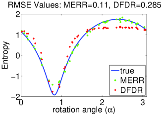
(a)

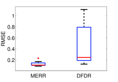
(b)

Figure 1: (a) Learned entropy of a one-dimensional marginal distribution of a rotated 2d Gaussian. Axes $x$: rotation angle in $[0,\pi]$. Axis $y$: entropy. (b) RMSE values of the MERR and DFDR algorithms. Boxplots are calculated from $25$ experiments.

From each $N(0,\Sigma_{u})$ distribution we sampled $500$ 2-dimensional i.i.d. points. From the $100$ sample sets, $25$ were used for training, $25$ for validation (i.e., selecting appropriate parameters), and $50$ points for testing. Our goal is to learn the entropy of the first marginal distribution: $H=\frac{1}{2}\ln(2\pi e\sigma^{2})$, where $\sigma^{2}=M_{1,1}$, $M=\Sigma_{u}\in\mathbb{R}^{2\times 2}$. Figure 1(a) displays the learned entropies of the $50$ test sample sets in a typical experiment. We compare the results of DFDR and MERR. One can see that the true and the estimated values are close to each other for both algorithms, but MERR performs better. The boxplot diagrams of the RMSE (root mean square error) values calculated from $25$ experiments confirm this performance advantage (Figure 1(b)). A reason why MERR achieves better performance is that DFDR needs to do many density estimations, which can be very challenging when the sample sizes are small. By contrast, the MERR algorithm does not require density estimation.

A.2.2 Aerosol prediction

Aerosol prediction is one of the largest challenges of current climate research; we chose this problem as a further testbed of our method. [35] pose the AOD (aerosol optical depth) prediction problem as a MIL task: (i) a given pixel of a multispectral image corresponds to a small area of $200\times 200m^{2}$, (ii) spatial variability of AOD can be considered to be small over distances up to $100km$, (iii) ground-based instruments provide AOD labels ($y_{i}\in\mathbb{R}$), (iv) a bag consists of randomly selected pixels within a $20km$ radius around an AOD sensor. The MIL task can be tackled using our MERR approach, assuming that (i) bags correspond to distributions ($x_{i}$), (ii) instances in the bag ($\{x_{i,n}\}_{n=1}^{N}$) are samples from the distribution.

We selected the MISR1 dataset [35], where (i) cloudy pixels are also included, (ii) there are $800$ bags with (iii) $100$ instances in each bag, (iv) the instances are 16-dimensional ($x_{i,n}\in\mathbb{R}^{16}$). Our baselines are the reported state-of-the-art EM (expectation-maximization) methods achieving average $100\times RMSE=7.5-8.5$ ($\pm 0.1-0.6$) accuracy. The experimental protocol followed the original work, where 5-fold cross-validation ($4\times 160$ ($160$) samples for training (testing)) was repeated $10$ times; the only difference is that we made the problem a bit harder, as we used only $3\times 160$ samples for training, $160$ for validation (i.e., setting the $\lambda$ regularization and the $\theta$ kernel parameter), and $160$ for testing.

• Linear $K$: In the first set of experiments, $K$ was linear. To study the robustness of our method, we picked $10$ different kernels ($k$) and their ensembles: the Gaussian, exponential, Cauchy, generalized t-student, polynomial kernel of order $2$ and $3$ ($p=2$ and $3$), rational quadratic, inverse multiquadratic kernel, Matérn kernel (with $\frac{3}{2}$ and $\frac{5}{2}$ smoothness parameters). The expressions for these kernels are

  $$k_{G}(a,b) =e^{-\frac{\left\|a-b\right\|_{2}^{2}}{2\theta^{2}}}, k_{e}(a,b) =e^{-\frac{\left\|a-b\right\|_{2}}{2\theta^{2}}}, k_{C}(a,b) =\frac{1}{1+\frac{\left\|a-b\right\|_{2}^{2}}{\theta^{2}}},$$

  $$k_{t}(a,b) =\frac{1}{1+\left\|a-b\right\|_{2}^{\theta}}, k_{p}(a,b) =\left(\left<a,b\right>+\theta\right)^{p}, k_{r}(a,b) =1-\frac{\left\|a-b\right\|_{2}^{2}}{\left\|a-b\right\|_{2}^{2}+\theta},$$

  $$k_{i}(a,b) =\frac{1}{\sqrt{\left\|a-b\right\|_{2}^{2}+\theta^{2}}}, k_{M,\frac{3}{2}}(a,b) =\left(1+\frac{\sqrt{3}\left\|a-b\right\|_{2}}{\theta}\right)e^{-\frac{\sqrt{3}\left\|a-b\right\|_{2}}{\theta}}$$

  $$k_{M,\frac{5}{2}}(a,b) =\left(1+\frac{\sqrt{5}\left\|a-b\right\|_{2}}{\theta}+\frac{5\left\|a-b\right\|_{2}^{2}}{3\theta^{2}}\right)e^{-\frac{\sqrt{5}\left\|a-b\right\|_{2}}{\theta}},$$

  where $p=2,3$ and $\theta>0$. The explored parameter domain was $(\lambda,\theta)\in\{2^{-65},2^{-64},\ldots,2^{-3}\}\times\{2^{-15},2^{-14},\ldots,2^{10}\}$; increasing the domain further did not improve the results.

  Our results are summarized in Table 4. According to the table, we achieve $100\times RMSE=7.91$ ($\pm 1.61$) using a single kernel, or $7.86$ ($\pm 1.71$) with ensemble of kernels (further performance improvements might be obtained by learning the weights).

  Table 4: Prediction accuracy of the MERR method in AOD prediction using different kernels: $100\times RMSE(\pm std)$. $K$: linear. The best single and ensemble predictions are written in bold.

  $k_{G}$	$k_{e}$	$k_{C}$	$k_{t}$	$k_{p}(p=2)$	$k_{p}(p=3)$
  $7.97$ ($\pm 1.81$)	$8.25$ ($\pm 1.92$)	$7.92$ ($\pm 1.69$)	$8.73$ ($\pm 2.18$)	$12.5$ ($\pm 2.63$)	$171.24$ ($\pm 56.66$)
  $k_{r}$	$k_{i}$	$k_{M,\frac{3}{2}}$	$k_{M,\frac{5}{2}}$	ensemble
  $9.66$ ($\pm 2.68$)	7.91 ($\pm\textbf{1.61})$	$8.05$ ($\pm 1.83$)	$7.98$ ($\pm 1.75$)	7.86 ($\pm\textbf{1.71}$)

• Nonlinear $K$: We also studied the efficiency of nonlinear $K$-s. In this case, the argument of $K$ was $\left\|\mu_{a}-\mu_{b}\right\|_{H}$ instead of $\left\|a-b\right\|_{2}$ (see the definition of $k$-s); for $K$ examples, see Table 1. Our obtained results are summarized in Table 5. One can see that using nonlinear $K$ kernels, the RMSE error drops to $7.90$ ($\pm 1.63$) in the single prediction case, and decreases further to $7.81$ ($\pm 1.64$) in the ensemble setting.

  Table 5: Prediction accuracy of the MERR method in AOD prediction using different kernels: $100\times RMSE(\pm std)$; single prediction case. $K$: nonlinear. Rows: kernel $k$. Columns: kernel $K$. For each row ($k$), the smallest RMSE value is written in bold.

  $k\backslash K$	$K_{G}$	$K_{e}$	$K_{C}$	$K_{t}$	$K_{M,\frac{3}{2}}$
  $k_{e}$	$8.14$ ($\pm 1.80$)	$8.10$ ($\pm 1.81$)	$8.14$ ($\pm 1.81$)	$\mathbf{8.07}$ ($\pm\mathbf{1.77}$)	$8.09$ ($\pm 1.88$)
  $k_{C}$	$7.97$ ($\pm 1.58$)	$8.13$ ($\pm 1.79$)	$7.96$ ($\pm 1.62$)	$8.09$ ($\pm 1.69$)	$\mathbf{7.90}$ ($\pm\mathbf{1.63}$)
  $k_{M,\frac{3}{2}}$	$8.00$ ($\pm 1.66$)	$8.14$ ($\pm 1.80$)	$8.00$ ($\pm 1.69$)	$8.08$ ($\pm 1.72$)	$\mathbf{7.96}$ ($\pm\mathbf{1.69}$)
  $k_{i}$	$8.01$ ($\pm 1.53$)	$8.17$ ($\pm 1.74$)	$8.03$ ($\pm 1.63$)	$7.93$ ($\pm 1.57$)	$8.04$ ($\pm 1.67$)
  $k\backslash K$	$K_{M,\frac{5}{2}}$	$K_{r}$	$K_{i}$	linear
  $k_{e}$	$8.14$ ($\pm 1.78$)	$8.12$ ($\pm 1.81$)	$8.12$ ($\pm 1.80$)	$8.25$ ($\pm{1.92}$)
  $k_{C}$	$7.95$ ($\pm 1.60$)	$7.92$ ($\pm 1.61$)	$7.93$ ($\pm 1.61$)	$7.92$ ($\pm 1.69$)
  $k_{M,\frac{3}{2}}$	$8.02$ ($\pm 1.71$)	$8.04$ ($\pm 1.69$)	$7.98$ ($\pm 1.72$)	$8.05$ $(\pm 1.83)$
  $k_{i}$	$8.05$ ($\pm 1.61$)	$8.05$ ($\pm 1.63$)	$8.06$ ($\pm 1.65$)	$\mathbf{7.91}(\pm\mathbf{1.61})$

Despite the fact that MERR has no domain-specific knowledge wired in, the results fall within the same range as [35]’s algorithms. The prediction is fairly precise and robust to the choice of the kernel, however polynomial kernels perform poorly (they violate our boundedness assumption).

References

- [1] Barnabás Póczos, Alessandro Rinaldo, Aarti Singh, and Larry Wasserman. Distribution-free distribution regression. AISTATS (JMLR W&CP), 31:507–515, 2013.
- [2] Thomas G. Dietterich, Richard H. Lathrop, and Tomás Lozano-Pérez. Solving the multiple instance problem with axis-parallel rectangles. Artificial Intelligence, 89:31–71, 1997.
- [3] Soumya Ray and David Page. Multiple instance regression. In ICML, pages 425–432, 2001.
- [4] Daniel R. Dooly, Qi Zhang, Sally A. Goldman, and Robert A. Amar. Multiple-instance learning of real-valued data. Journal of Machine Learning Research, 3:651–678, 2002.
- [5] Andrea Caponnetto and Ernesto De Vito. Optimal rates for regularized least-squares algorithm. Foundations of Computational Mathematics, 7:331–368, 2007.
- [6] Ingo Steinwart and Andres Christmann. Support Vector Machines. Springer, 2008.
- [7] David Haussler. Convolution kernels on discrete structures. Technical report, Department of Computer Science, University of California at Santa Cruz, 1999. (http://cbse.soe.ucsc.edu/sites/default/files/convolutions.pdf).
- [8] Fei Wang, Tanveer Syeda-Mahmood, Baba C. Vemuri, David Beymer, and Anand Rangarajan. Closed-form Jensen-Rényi divergence for mixture of Gaussians and applications to group-wise shape registration. Medical Image Computing and Computer-Assisted Intervention, 12:648–655, 2009.
- [9] Risi Kondor and Tony Jebara. A kernel between sets of vectors. In ICML, pages 361–368, 2003.
- [10] Tony Jebara, Risi Kondor, and Andrew Howard. Probability product kernels. Journal of Machine Learning Research, 5:819–844, 2004.
- [11] Frank Nielsen and Richard Nock. A closed-form expression for the Sharma-Mittal entropy of exponential families. Journal of Physics A: Mathematical and Theoretical, 45:032003, 2012.
- [12] Shaohua Kevin Zhou and Rama Chellappa. From sample similarity to ensemble similarity: Probabilistic distance measures in reproducing kernel Hilbert space. IEEE Transactions on Pattern Analysis and Machine Intelligence, 28:917–929, 2006.
- [13] Bernhard Schölkopf and Alexander J. Smola. Learning with Kernels: Support Vector Machines, Regularization, Optimization, and Beyond. MIT Press, 2002.
- [14] Marco Cuturi, Kenji Fukumizu, and Jean-Philippe Vert. Semigroup kernels on measures. Journal of Machine Learning Research, 6:1169–1198, 2005.
- [15] André F. T. Martins, Noah A. Smith, Eric P. Xing, Pedro M. Q. Aguiar, and Mário A. T. Figueiredo. Nonextensive information theoretical kernels on measures. Journal of Machine Learning Research, 10:935–975, 2009.
- [16] Matthias Hein and Olivier Bousquet. Hilbertian metrics and positive definite kernels on probability measures. In AISTATS, pages 136–143, 2005.
- [17] Barnabás Póczos, Liang Xiong, and Jeff Schneider. Nonparametric divergence estimation with applications to machine learning on distributions. In UAI, pages 599–608, 2011.
- [18] Barnabás Póczos, Liang Xiong, Dougal Sutherland, and Jeff Schneider. Support distribution machines. Technical report, Carnegie Mellon University, 2012. (http://arxiv.org/abs/1202.0302).
- [19] Junier B. Oliva, Willie Neiswanger, Barnabás Póczos, Jeff Schneider, and Eric Xing. Fast distribution to real regression. AISTATS (JMLR W&CP), 33:706–714, 2014.
- [20] Junier Oliva, Barnabás Póczos, and Jeff Schneider. Distribution to distribution regression. ICML (JMLR W&CP), 28:1049–1057, 2013.
- [21] László Györfi, Michael Kohler, Adam Krzyzak, and Harro Walk. A Distribution-Free Theory of Nonparametric Regression. Springer, New-york, 2002.
- [22] Samory Kpotufe. k-NN regression adapts to local intrinsic dimension. Technical report, Max Planck Institute for Intelligent Systems, 2011. (http://arxiv.org/abs/1110.4300).
- [23] Thomas Gärtner, Peter A. Flach, Adam Kowalczyk, and Alexander Smola. Multi-instance kernels. In ICML, pages 179–186, 2002.
- [24] Alain Berlinet and Christine Thomas-Agnan. Reproducing Kernel Hilbert Spaces in Probability and Statistics. Kluwer, 2004.
- [25] Yasemin Altun and Alexander Smola. Unifying divergence minimization and statistical inference via convex duality. In COLT, pages 139–153, 2006.
- [26] Arthur Gretton, Karsten M. Borgwardt, Malte J. Rasch, Bernhard Schölkopf, and Alexander Smola. A kernel two-sample test. Journal of Machine Learning Research, 13:723–773, 2012.
- [27] Bharath K. Sriperumbudur, Kenji Fukumizu, and Gert R. G. Lanckriet. Universality, characteristic kernels and RKHS embedding of measures. Journal of Machine Learning Research, 12:2389–2410, 2011.
- [28] Kenji Fukumizu, Francis Bach, and Michael Jordan. Dimensionality reduction for supervised learning with reproducing kernel Hilbert spaces. Journal of Machine Learning Research, 5:73–99, 2004.
- [29] Andreas Christmann and Ingo Steinwart. Universal kernels on non-standard input spaces. In NIPS, pages 406–414, 2010.
- [30] Krikamol Muandet, Kenji Fukumizu, Francesco Dinuzzo, and Bernhard Schölkopf. Learning from distributions via support measure machines. In NIPS, pages 10–18, 2012.
- [31] Larry Wasserman. All of Nonparametric Statistics. Springer, 2006.
- [32] Felipe Cucker and Steve Smale. On the mathematical foundations of learning. Bulletin of the American Mathematical Society, 39:1–49, 2002.
- [33] Christian Berg, Jens Peter Reus Christensen, and Paul Ressel. Harmonic Analysis on Semigroups. Springer-Verlag, 1984.
- [34] Bharath Sriperumbudur, Arthur Gretton, Kenji Fukumizu, Gert Lanckriet, and Bernhard Schölkopf. Hilbert space embeddings and metrics on probability measures. Journal of Machine Learning Research, 11:1517–1561, 2010.
- [35] Zhuang Wang, Liang Lan, and Slobodan Vucetic. Mixture model for multiple instance regression and applications in remote sensing. IEEE Transactions on Geoscience and Remote Sensing, 50:2226–2237, 2012.
- [36] Yuchen Zhang, John C. Duchi, and Martin J. Wainwright. Divide and conquer kernel ridge regression: A distributed algorithm with minimax optimal rates. Technical report, University of California, Berkeley, 2014. (http://arxiv.org/abs/1305.5029).
- [37] Zoltán Szabó, Bharath Sriperumbudur, Barnabás Póczos, and Arthur Gretton. Learning theory for distribution regression. Technical report, Gatsby Unit, University College London, 2014. (http://arxiv.org/abs/1411.2066).
- [38] Michael Reed and Barry Simon. Methods of Modern Mathematical Physics – Functional Analysis. Academic Press, 1980.
- [39] Gabriel Nagy. Real analysis (lecture notes): Chapter III: Measure theory, Section 3: Measurable spaces and measurable maps. Technical report, Kansas State University. (http://www.math.ksu.edu/~nagy/real-an/3-03-measbl.pdf).
- [40] K.R. Parthasarathy. Probability Measures on Metric Spaces. Academic Press, 1967.
- [41] John L. Kelley. General Topology. Springer, 1975.
- [42] John Shawe-Taylor and Nello Cristianini. Kernel Methods for Pattern Analysis. Cambridge University Press, 2004.
- [43] Zoltán Szabó. Information theoretical estimators toolbox. Journal of Machine Learning Research, 15:283–287, 2014.