Cosmological model with variable vacuum pressure
Abstract
Scenarios of the cosmological evolution are studied by using an equation of state (EoS) having points where the specific enthalpy of the cosmological fluid vanishes. A large class of barotropic EoS’s admits, depending upon initial conditions, analogues of the “Big Rip”, as well as solutions describing exponential inflation followed by usual matter dominance; their classification is proposed. We discuss extensions to more general two-parametric EoS dealing with a pre-inflationary evolution and yielding stages with both increasing and decreasing energy density as a function of time. Possible cosmological scenarios with transitions from collapse to an expanding Universe or a closed oscillating one, without reaching a singularity are included.
pacs:
98.80.CqI Introduction
The Standard Cold Dark Matter cosmological model with (CDM model) describes a huge amount of observational data WMAP ; Plank that determine the cosmological fraction of the baryonic matter, the cold dark matter and the dark energy. On the other hand, the CDM model leads to the well-known problems of horizon and of spatial flatness (see, e.g. Weinberg ; Linde ). These problems are currently resolved by introducing the inflationary period inflation in the early Universe, leading to a high degree of isotropy of the cosmic microwave background and spatial flatness. This can be achieved either within modifications of General Relativity or by taking into account some additional physical fields Sahni ; Linde , which are manifest at cosmological scales.
Traditionally, the bulk of matter in the Universe is represented by a sum of baryonic matter, unknown dark matter (DM) with zero (or very small) pressure and dark energy (DE). In the hydrodynamical picture, the total pressure is a sum . This picture can be complemented by introducing a cosmological (e.g., scalar) field. On the other hand, at present there are no theoretical arguments that could single out a unique scalar field potential, a Lagrangian of a modified gravitation theory etc. In this situation, qualitative considerations of cosmological scenarios often use a phenomenological equation of state (EoS) describing on the average the whole matter in terms of the local frame energy density and other thermodynamical parameters (see eos_models and references therein). A widely accepted model for the dark energy is a homogeneous perfect fluid with . Cosmic acceleration requires that ; recent WMAP and Planck results WMAP ; Plank are consistent with the value , however “phantom DE”, for which BigRip , is not completely ruled out phantom .
A number of generalizations dealingwith either explicit forms of EoS or having a parametric form exist eos_models . In this paper we use an EoS containing a contribution from ordinary matter with a linear part , (e.g., due to “hot” matter with ) and a nonlinear term depending on the total energy density . This EoS is inspired by the well-known bag models of the quark-hadron (de)confinement phase transition when quarks and gluons coagulate to form hadrons (see, e.g., Shurik ; JKS ; JKS1 ). These models involve the so called “bag” pressure constant that can be interpreted as the effect of the quantum-chromodynamical vacuum. A generalization in which the constant is replaced by an increasing function of temperature , was suggested by Källman Kallman . This modification of the EoS was re-derived and its hydrodynamical and cosmological consequences have been discussed in a number of papers (see JKS ; JKS1 ; ECh and references therein). The possibility that a small fraction of colored objects escape hadronization, surviving as islands of free coloured particles, called quark nuggets was studied e.g. in Ref. Odessa .
Possible variation of the cosmological constant with temperature or energy density was discussed e.g. in Ref. Lambda . Of interest is the connection of this phenomenon with the variable quark bag “constant” considered in the present paper. Below we extend the idea of the variable vacuum pressure to very early times of the Universe, although we do not exclude that the nonlinear part of the equation of state can have different origin. We assume that may be a function of . This is applied to equations of the homogeneous isotropic Universe (Section II) dealing with a barotropic EoS. In Section III we discuss more general equations of state that involve two thermodynamical parameters, namely, the energy density and the specific volume. The results are summarized in Section IV.
II Hydrodynamical models of cosmological evolution
II.1 Preliminaries: homogeneous isotropic cosmology
Let us write the Friedmann equations for a homogeneous and isotropic Universe for the FLRW metric
| (1) |
where is the scale factor, is the distance element on the unit sphere, for the closed Universe, for open one, and for spatially flat models; correspondingly, in what follows .
The Friedmann equations for the scale factor are
| (2) |
where in case of a hydrodynamical cosmological models stands for the energy density of all kinds of matter in the Universe and is the effective pressure111We use the system of units in which and .;
| (3) |
where . Here we do not introduce explicitly the cosmological constant, because it can be incorporated in and as “dark energy” with EoS ; we remind that the present-day value of (from CDM cosmological model) can be neglected for the redshifts or greater. For our purposes it is sufficient to use only Eq. (3) as we further use the hydrodynamical equation
| (4) |
or
| (5) |
where and is the specific enthalpy. With account for (3) we have
| (6) |
where in the case of the expanding Universe and in case of the contracting one. In what follows we assume for .
II.2 Barotropic equation of state
The above equations must be complemented by an EoS. We use the analogy with the quark bag model, where the bag pressure can be interpreted as the effect of the quantum-chromodynamical vacuum. Similarly, for energy densities at very early stages of the cosmological evolution, we assume that there was a strong negative bag pressure inherent of the cosmological vacuum for all physical interactions.
In generalizations of the quark bag model Kallman ; JKS , the bag constant is replaced by a function of temperature , so that . In the standard bag model, the first term of this equation describes the ultra-relativistic gas. Introduction of temperature as an independent variable is preferable in case of thermodynamical equilibrium, because it enables us to characterize different components of the cosmological fluid by the same parameter . On the other hand, in qualitative considerations of cosmological problems it is more convenient to introduce an effective EoS in terms of energy density .
Let us start with the barotropic EoS
| (7) |
where we assume that and the corresponding term represents an input of an “ordinary” matter, e.g., for the hot matter (ultra-relativistic gas). We write the “vacuum pressure” as , and we assume that is a monotonically increasing function. We suppose, for simplicity, that , so that for small densities the effect of the vacuum pressure be negligible 222Consistency with the CDM cosmological model for small densities (e.g., for the present era) requires the addition of a positive constant to .. Equation (4) then assumes the form
| (8) |
The crucial point is the existence of some value where the specific enthalpy vanishes, i.e. ; this will be asumed in what follows. We see from (8) that the behavior of the trajectories in the plane near do not depend on the choice of . However, contrary to the cases of and , for , the trajectories cannot be always extended to all positive values of , and this requires additional considerations (see below).
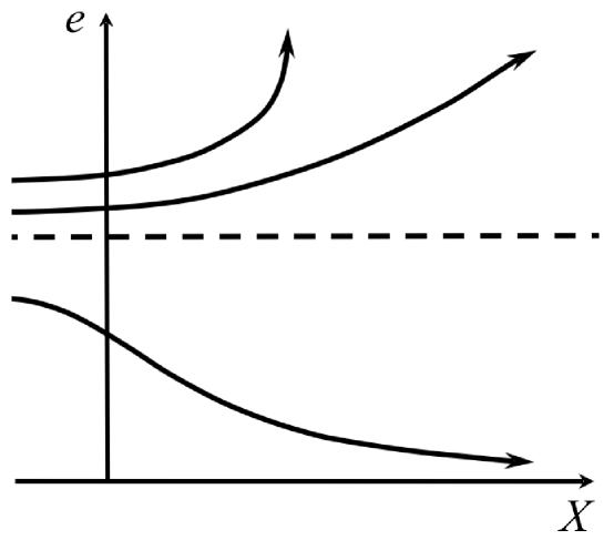
We now describe types of the qualitative behavior of solutions of equation (8) in more details. For they are illustrated in Fig. 1 in case of the expansion (S=1) of the spatially flat Universe.
A1: The solutions are represented by the lower curve in Fig. 1 lying completely in the domain of variables such that . For we have , and this corresponds to a long period of an exponential inflation. As increases, the energy density decreases, and the contribution of the vacuum pressure becomes negligible. This is, however, the consequence of condition and it can be easily corrected if we want to take into account the present value of .
A2: The solutions are represented by the curve lying in the second region, , between the other curves in Fig. 1. For such a solution is defined for all , this function is monotonically increasing up to infinity; and are defined for all . This scenario takes place, e.g., in case of a bounded .
A3: The solutions are represented by the top curve in Fig. 1 lying in the region , with a “runaway” behavior like that of the Big Rip BigRip . A solution of this type blows up at some finite time, and it cannot be extended for all and/or all . Such a behavior333To save the space we show the trajectories corresponding to different kinds of in the same figure. occurs, e.g., if we suppose that grows faster than , for large .
An example with explicit EoS and analytic solutions is given in Appendix A.
For we always have ; therefore the qualitative situation is analogous to the previous case. For () we have the same dependence described by Fig. 1 because Eqs. (5) and (8) do not contain . There can be either A1, A2 or A3 as possible cases for , though they can yield different asymptotical behavior for and for or .
It is easy to see, in virtue of (3), that, since as , we have . In the region all the solutions are monotonically decreasing functions and for . In case of a fine tuning, if, at some , we have sufficiently close to , this closeness will remain during a long time; then in virtue of (3) , where , whence . In the second region, , the situation is also the same as for : we have either the “runaway” solutions A3 or solutions A2.
In both cases, and , the line is a solution; other solutions (either from the region or from the region ), cannot cross this line444It would contradict the uniqueness of the solution of (8) with initial condition at some initial point..
: Since the right hand side of equation (3) must be positive, the trajectories are located to the right of the curve . The intersections of solutions of equation (8) with this curve typically correspond to simple zeros555This is a simple zero unless at this point , i.e. simultaneously with . In the latter case the solution spends an infinite time near this point. of function ; therefore, they describe turning points of solutions to equation (3) that can be rewritten as
| (10) |
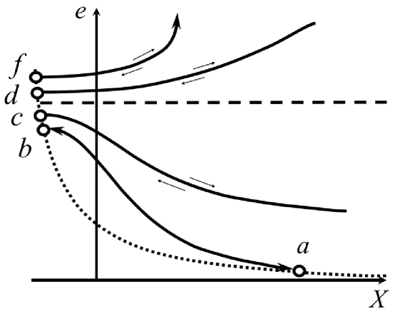
Any turning point in its neighborhood relates two branches of the cosmological evolution with different signs of : from a contracting () to an expanding ) Universe. The mutual arrangement of the trajectories of (8) in the plane (Fig. 2) shows that there must be at least one intersection of any trajectory with the curve of turning points . Correspondingly, possible types of solutions are as follows.
A4: Oscillating solutions in the domain for . On account for as , due to equation (8), we have . Therefore, for a solution that starts, e.g. at the turning point of the solution , there is necessarily another turning point () (see Fig. 2). There is then an oscillating solution of () described by the curve between points and ; in this model oscillates without reaching any singularity.
For , depending on initial conditions, one can also have an oscillatory behavior like A4. On the other hand, in this case an alternative version with ever expanding Universe is possible:
A5: monotonically decreasing solutions , such as those starting from the turning point in Fig. 2 and existing for all to the right of the turning point . Here a contraction () is followed by expansion ( as ); the singularity is not reached and remains finite for any time.
In the region we have a monotonically increasing solution of equation (8). Similarly to A2 and A3, we have two possibilities.
A6: Solutions that are represented by trajectories that have a turning point (like in Fig.2) and tend to infinity as . For and , as functions of , we have transition from contraction to expansion at .
A7: Solutions with a transition from contraction to expansion at some turning point ( in Fig.2, upper curve); these solutions blows up at some finite .
Ending this Section, we note that if we have two zero points of enthalpy666provided we do not assume to be monotonic., i.e. and such that and ; consequently we get a family of solutions with for and for . In this case can be interpreted as a modern value of the dark energy density described by .
II.3 Monotonically decreasing
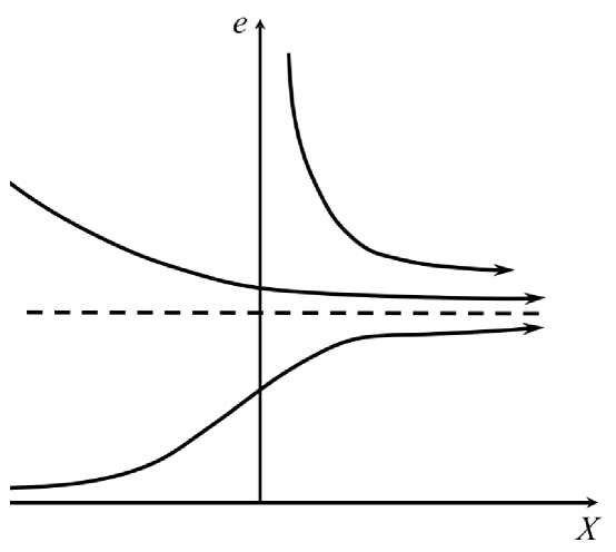
For completeness, we consider also the case of monotonically decreasing function with the same relation for ; we suppose that there exists such that and therefore . Then in the domain we have along the trajectories, and for we have . The behavior of the trajectories is shown in Figs. 3, 4. The qualitative types of the solutions of (8) are as follows.
B1 (): Solutions in the domain : defined on , for , and for .
B2 (): Solutions defined on and we have for , and for . This is possible, e.g., in case of a bounded ; for we have the same asymptotic behavior of , both for and . This kind of behavior is appropriate for the classical CDM cosmological models with or (see, e.g. Weinberg ; Dinverno ).
B3: Solutions defined for , where as (”Big Rip in the past”, upper curve in Fig. 3). For this type is possible, e.g., if for and grows faster than , . For we have .
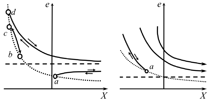
The next six types of solutions of (8), shown in Fig. 4, deal with the closed Universe (); B4, B5, B6 describe solutions with bounded energy density (Fig. 4, left panel) and B7, B8, B9 are solutions with unbounded (Fig. 4, right panel).
B4 (): Monotonically increasing in the domain with turning point ().
B5 (): Oscillating solution (between and ).
B6 (): Monotonically decreasing in the domain with turning point ().
Fig. 4, right panel:
B7 (): Unbounded monotonically decreasing in the domain with turning point ; as . The Universe starts with infinite , whereupon expansion is replaced by contraction after passing the turning point .
B8 (): Unbounded monotonically decreasing in the domain , defined for all ; as ; as .
B9 (): Unbounded monotonically decreasing in the domain , for ; as ; as .
Note that one can easily extend the results of subsections II.2 and II.3 to the case of negative and . In this case we have the same types of trajectories as those shown in Figs. 1–4.
III Generalization: two-parametric EoS
In the preceding section we have used the fact that the solution of the first order differential equation (8) cannot cross the line , since this is also a solution of (8). However, it is interesting to consider scenarios when the sign of may change during the cosmological evolution. To this end we relax the conditions of the preceding section and assume that the EoS depends on two independent thermodynamical variables. On the other hand, one can expect that, if the dependence of the pressure on the additional variable, besides , is weak, the cosmological evolution will be very close to that of the preceding Section and a solution that crosses zero points of will spend a considerable time near these points (and thus can invoke a kind of the exponential inflation).
In this Section, instead of Eq. (8), we prefer to deal directly with Eq. (5), where , , is the proper frame baryon number density. Due to baryon conservation, in case of metric (1), we have
| (11) |
where are the values at some .
Instead of the straight line , we suppose that there is (only) one curve where the specific enthalpy vanishes. Obviously, in the general case, the function does not satisfy (5) and some trajectories of solutions can cross this curve. The most simple extension of the corresponding assumptions of Section II.2 is that the function is defined for all and it is a monotonic function. The trajectories slightly differ for different signs of monotonicity. There are four possibilities: (C1) is monotonically increasing, for ; (C2) the same sign of monotonicity, but for ; (C3) is monotonically decreasing, for ; (C4) the same sign of monotonicity as in (C3), but for .
Possible trajectories of the system (3)-(5) that do not cross the curve are qualitatively the same as those of Section II, so we concentrate on types of trajectories for which the sign of changes, as shown schematically in Fig. 5. These scenarios of cosmological evolution differ considerably from the standard pictures described in the textbooks (see, e.g., Dinverno , Fig. 23.1). The trajectories that do not cross the curve are not shown in Fig. 5; for example, in case of C1, there may be infinite solutions that move to the area above the curve .
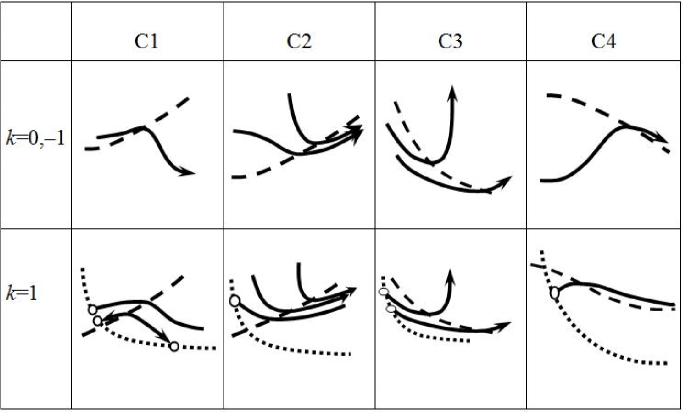
In any case, for the initially expanding Universe will expand forever. In case of the closed Universe (), for some solutions, there is a possibility of return to a contraction; there can be also periodic solutions and solutions with return from contraction to expansion.
It is interesting to note that there are scenarios when increases and then decreases either to zero or to some constant value (see Fig. 5, C1 and C4). Any more complete description may be obtained only if more information about is provided. Two concrete examples with types C1 and C4 are presented in Appendix B.
IV Conclusions
We have investigated a class of nonlinear equations of state that have points of zero enthalpy; to do so, we used general qualitative properties known from the theory of ordinary differential equations. In the case of the barotropic EoS occurrence of such point leads to the possibility of a period of rapid expansion with almost constant energy density. Under appropriate initial conditions, this period can last as long as needed to provide the necessary size of the causally connected regions in future, ensuring, e.g., an adequate solution to the well-known problem of horizon etc.
Under general assumptions, we have classified possible cosmological scenarios, including a number of those without the cosmological singularity. In case of an open and spatially flat metrics, the Universe expands either forever or undergoes a Big Rip. In case of the closed Universe there can be also transitions from collapse to expansion or vice versa. A closed oscillating Universe without reaching a singularity is also possible.
Our findings deal with simple EoS allowing to discuss different scenarios of the early cosmological evolution. Nevertheless, if we assume that these considerations have relevance to reality, one can speculate on why our Universe starts with small deviations from the state with zero enthalpy, for example due to quantum fluctuations near this state. These fluctuations can start either “phantom” cosmological evolution leading to a kind of the Big Rip, or “normal” expansion with a transition to the standard CDM model described in textbooks (see, e.g., Weinberg ). To have a sufficiently long period of inflation, a kind of fine tuning is required (e.g., approach to the point ), compelling to invoke a sort of the anthropic principle. However, such a tuning is not more restrictive than, e.g., the use of equation of state with .
The above-mentioned requirement of the fine tuning is relaxed if we consider a two-parametric EoS. In this case, an infinity of solutions crossing states with zero enthalpy may exist; and there is an immense freedom in choosing the evolution as the scale factor . In case of a sufficiently weak dependence of on it is natural to assume that the behavior of trajectories near points of zero enthalpy will be similar to that of Section II.2 and there is a sufficiently long period of inflation.
Furthermore, one may speculate about a multi-component fluid. We know that at present some form of DE dominates, but moving back in time its fraction becomes negligible (within the framework of the CDM model). On the other hand, for very early (post-Planckian) times, the other form of DE must have dominated to provide inflation. Within such a scenario, one may have different inflation epochs corresponding to the domination of different DE components (cf. multiple stages of inflation in Ref. schism ). This is consonant with the idea of the existence of a “mini-inflation” due to the existence of metastable states in strongly interacting matter JKS ; JKS1 , see also Shurik . However, any smooth interpolation between these different inflation epochs remains a challenge for the theory.
Acknowledgments
We thank the referee for her/his helpful comments. We are grateful to G. Stelmakh for his help in preparing our figures. L. J. was supported by the National Academy of Sciences of Ukraine, Department of Astronomy and Physics programme “Matter Under Extreme Conditions”. V.I.Z. was supported by the Taras Shevchenko National University of Kyiv, scientific program “Astronomy and Space Physics”.
Appendix A “Equivalent” scalar field potential
It is important to have a scalar field analogue of the hydrodynamical models in question. Here we present an analytic example dealing with a special form of the EoS and an ”equivalent” scalar field description yielding the same evolution of the scaling factor.
It is well known that in case of the homogeneous isotropic cosmology, one can find a scalar field Lagrangian that mimics the hydrodynamical evolution (see, e.g., Zhdanov ; Odintsov2 ; Chavanis and references therein). Here we consider the scalar field equations giving the same evolution of the “observable” space-time geometry, i.e. the same dependence , as that following from EoS . Consider the scalar field Lagrangian with the standard kinetic term
| (12) |
The corresponding energy-momentum tensor is
| (13) |
In case of a homogeneous isotropic cosmology with the metric (1), it has the form of the hydrodynamical energy-momentum tensor with the following energy density and pressure:
| (14) |
Combining Eqs. (14) with Eq. (2,3) we obtain a parametric representation of the “equivalent” scalar field potential:
| (15) |
| (16) |
In the case of barotropic EoS, such as (7), and spatially flat Universe (), it is more convenient to look for a parametric representation of the form , . Combining with Eq.(4) we get whence
| (17) |
yielding the potential in a parametric form.
There is a number of analytic examples describing the cosmological evolution in various dynamical DE models (see, e.g. eos_models ; Odintsov2 ; Chavanis ). Below we use particular examples to illustrate the general statements of the previous sections.
In case of , we have an EoS of the form
| (18) |
In this case equation (8) with the initial condition for can be easily integrated:
| (19) |
It is also possible to find an analytic form of . Equation (17) yields
| (20) |
where is an integration constant. The inverse function is
Substitution into (14) yields
| (21) |
This is the potential that ensures the same dependence of the scale factor as the EoS (18).
Appendix B Two examples
Lacking reliable knowledge about the equation of state in the very early epoch, below we consider, for illustration purposes, simple examples of C1 and C4 types, . The solutions for can be easily analyzed using these pictures by superimposing the line onto the graph and taking into account the turning points. Assuming Eq. (7), we set . Then . The solutions of equation (5) are calculated for most simple cases: (i) , (Fig. 6); (ii) , (Fig. 7). On the figures we show only those trajectories that cross the line where changes its sign.
In case of (i) all solutions crossing the curve , tend to for . Besides, there are monotonically increasing solutions (not shown in Fig. 6) below the curve with the same asymptotic behavior for . For large negative , the solutions lead to nonphysical values .
In case of (ii) all solutions after crossing the curve tend to zero for . However, there are also solutions (not shown in Fig. 7) to the left of the curve tending to infinity for at some finite .


References
- (1) G. Hinshaw, D. Larson, E. Komatsu et al., Nine-year Wilkinson Microwave Anisotropy Probe (WMAP) Observations: Cosmological Parameter Results, ApJ Suppl., 208, 25 (2013), arXiv:1212.5226.
- (2) Planck Collaboration: Planck 2013 results. XVI. Cosmological parameters (2013), arXiv:1303.5076.
- (3) S. Weinberg, Cosmology, Oxford Univ. Press, 2008.
- (4) A. Linde, Particle Physics and Inflationary Cosmology, Contemp. Concepts Phys. 5, 1 (2005), arXiv:hep-th/0503203; A. Linde, Inflationary Cosmology, Lect. Notes Phys. 738:1-54 (2008), arXiv:0705.0164v2.
- (5) A. A. Starobinsky, Phys. Lett. B91, 99 (1980): A. H. Guth, Phys. Rev. D 23, 347 (1981); A. Albrecht, P. Steinhardt, Phys. Rev. Lett. 48, 1220 (1982); A. D. Linde, Phys. Lett. B108, 389 (1982).
- (6) V. Sahni, Classical and Quantum Gravity, 19, 3435 (2002).
- (7) E. V. Linder, R. J. Scherrer, Phys. Rev. D 80, 023008 (2009); S. Nojiri, S. D. Odintsov, Phys. Rev. D72, 023003 (2005) (hep-th/0505215); S. Nojiri, S. D. Odintsov, Phys. Lett. B639, 144 (2006); S. Capozziello, V. Cardone, E. Elizalde, S. Nojiri, S. D. Odintsov, Phys. Rev. D 73, 043512 (2006); L. Xu, Y. Chang, arXiv:1310.1532; M. Li, X.-D. Li, Y.-Zh. Ma, X. Zhang, Zh. Zhang, arXiv:1305.5302; P.-H. Chavanis, Eur. Phys. J. Plus 129 38 (2014).
- (8) K. Bamba, S. Capozziello, S. Nojiri, S. D. Odintsov, Astrophys.Space Sci. 342, 155 (2012); arXiv:1205.3421.
- (9) P.-H. Chavanis, arXiv:1309.5784 (2013)
- (10) R. R. Caldwell, M. Kamionkowski, and N. N. Weinberg, Phys. Rev. Lett. 91 (2003) 071301; arXiv:astro-ph/0302506.
- (11) B. Novosyadlyj, O. Sergijenko, R. Durrer, V. Pelykh, Physical Review D 86, 083008 (2012).
- (12) L. Jenkovszky and A. A. Trushevsky, Nuovo Cimento 34A, 369 (1976); A. I. Bugrij and A. A. Trushevsky, JETP 73, 3 (1977); L. L. Jenkovszky and A. N. Shelkovenko, Nuovo Cim. A101 137 (1989).
- (13) L. Jenkovszky, B. Kämpfer and V. Sysoev, Supercooled, metastable quark-gluon plasma universe, Yad. Fizika 50 (1989) 1747.
- (14) L. Jenkovszky, B. Kämpfer and V. Sysoev, Z. Phys. C - Particles and Fields 48, 147 (1990).
- (15) C. G. Källman, Phys, Lett. 134B, 363 (1984).
- (16) V. Boyko, L. Jenkovszky, V. Sysoev, Soviet Journal of Particles and Nuclei (EChAYa) 22, 675 (1991).
- (17) M. Brilenkov, M. Eingorn, L. Jenkovszky, and A. Zhuk, JCAP 08, 002 (2013), arXiv:1304.7521.
- (18) J. E. Felten, Rev. Mod. Phys. 58, 689 (1986); J. M. Overduin and F. I. Cooperstock, Phys. Rev. D 58, Is.4 (1998), id. 043506 astro-ph/9805260; A. Silbergleit, astro-ph/0208465; U. Mukhopadhyay, and S. Ray, N. B. U. Math. J. II, 51 (2009) arXiv:astro-ph/0510554; S. Ray, U. Mukhopadhyay and X.-H. Meng, Grav.Cosmol. 13 142 (2007), arXiv:astro-ph/0407295; Zh. Li-juan, M. Wei-xing, and L. Kisslinger, J. Mod. Phys. 3 1172 (2012), astro-ph/arXiv:1204.3084.
- (19) R. D’Inverno. Introducing Einstein’s Relativity. Oxford Univ. Press, 1998.
- (20) A. Ijjas,P.J. Steinhardt, A. Loeb, arXiv:1402.6980 (2014).
- (21) V. I. Zhdanov and G. Yu. Ivashchenko, Kinematics and Physics of Celestial Bodies, 25, 73 (2009); arXiv:0806.4327.