Flows in Complex Networks: Theory, Algorithms, and Application to Lennard-Jones Cluster Rearrangement

Abstract.

A set of analytical and computational tools based on transition path theory (TPT) is proposed to analyze flows in complex networks. Specifically, TPT is used to study the statistical properties of the reactive trajectories by which transitions occur between specific groups of nodes on the network. Sampling tools are built upon the outputs of TPT that allow to generate these reactive trajectories directly, or even transition paths that travel from one group of nodes to the other without making any detour and carry the same probability current as the reactive trajectories. These objects permit to characterize the mechanism of the transitions, for example by quantifying the width of the tubes by which these transitions occur, the location and distribution of their dynamical bottlenecks, etc. These tools are applied to a network modeling the dynamics of the Lennard-Jones cluster with 38 atoms (${\rm LJ}_{38}$) and used to understand the mechanism by which this cluster rearranges itself between its two most likely states at various temperatures.

1. Introduction

In recent years, networks have gained popularity as a tool to represent, organize, and interpret phenomena arising in many fields of science, including physics, biology, social sciences, etc. Questions as diverse as the structure of the World Wide Web, the robustness of a nation’s banking system or its power grid, or the mechanism of functions inside a cell can be expressed in terms of networks. These applications have led to networks whose structure and complexity have gone far beyond the examples studied before in the classical computer science literature. Driven partly by the emergence of these new applications, research in network science has also undergone a revolutionary change in recent years. While traditional network science was basically a subject of graph theory and focused on networks with rather simple structure, recent studies often took the viewpoint of treating networks as complex systems, and used tools and concepts from statistical mechanics. While the structure and topology of networks has been under much investigation, the dynamics on the network is less well understood despite the fact that it leads to important and nontrivial questions. For example, any network with positive-weighted edges defines a Markov jump process (MJP) (and vice versa) and in many applications, it is of interest to understand the interplay between the network structure and the dynamics of this MJP. Our aim here is to address such questions within the framework of transition path theory (TPT), originally introduced in [17] (see also [32, 18] for reviews) and already used in [26] in the context of networks and MJPs – the present work can be viewed as a continuation of this last paper. In a nutshell, the basic idea in TPT is to single out two specific sets of nodes and analyze the statistical properties of the reactive trajectories by which transitions between these sets occur – if the sets are chosen appropriately, this permits to extract the most salient features of the dynamics on the network and relate them to its topology. This is like probing an electrical network by wiring it at different locations and analyzing how the current flow from the nodes wired positively to those wired negatively [15, 4, 13].

TPT is also related to the potential-theoretic approach to metastability championed by Bovier and collaborators [6, 7, 8, 9], albeit the emphases of both approaches are different. The potential-theoretic approach has been introduced as a theoretical tool to obtain rigorous bounds on the low-lying eigenvalues that characterize the slowest relaxation phenomena in MJPs displaying metastability [12, 20, 30]. TPT on the other hand permits to characterize exactly the statistical properties of the transition pathways on complex networks that are not necessarily metastable, or such that the low-lying part of their spectrum is too complicated to be estimated analytically. Importantly TPT can also be used as a computational tool in such situations. By being able to analyze the flow of transitions between specific parts of the network, for example by generating numerically reactive trajectories by which these transitions occur, or even no-detour transitions paths, and analyzing their statistical properties, TPT can provide invaluable information about the network and the dynamics it supports.

(a)          (b)

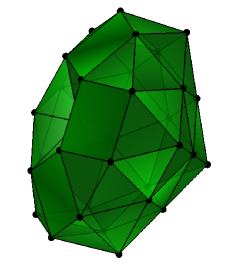
Figure 1. The two lowest minima of the potential energy of the LJ₃₈. (a): The face-centered cubic truncated octahedron with the point group $O_{h}$ is the lowest minimum. (b): The icosahedral structure with the $C_{5v}$ point group is the second lowest minimum. Throughout this paper we refer to them as FCC and ICO, respectively.

To make this last point and illustrate the usefulness of the tools developed in this paper, we will apply them to analyze the network developed by David Wales and collaborators to model the dynamics of Lennard-Jones clusters with 38 atoms (${\rm LJ}_{38}$) [16, 38]. ${\rm LJ}_{38}$ is a prototypical example illustrating how the complexity of a system’s energy landscape (and its associated network) affects its dynamical properties, a feature that is also observed in other complex phenomena such as protein folding or glassy dynamics. ${\rm LJ}_{38}$ has a double-funnel landscape: its global minimum, a face-centered-cubic truncated octahedron, lies at the bottom of one funnel, whereas its second lowest minimum, an incomplete Mackay icosahedron, lies at the bottom of the other (see Fig. 1). The deeper octahedral funnel is also narrower, and believed to be mostly inaccessible from the liquid state. Thus, when ${\rm LJ}_{38}$ self-assembles by crystallization, it does so by reaching the bottom of the shallow but broader isocahedral funnel, and an interesting question is how does ${\rm LJ}_{38}$ manage to subsequently find its ground state structure by travelling from the shallow funnel to the deep one? This question of rearrangement is the one that we will address below. It is made complicated by the ruggedness of the energy landscape of ${\rm LJ}_{38}$, which has an enormous number of local minima separated by a hierarchy of barriers of different heights.

The remainder of this paper is organized as follows. In Sec. 2 we summarize the main outputs of TPT. In Sec. 3 we introduce sampling tools based on the theory. In Sec. 4 we discuss the case of metastable networks, and establish connections between TPT and the potential theoretic approach to metastability as well as large deviation theory that arise in these situations. In Sec. 5 we apply the tools introduced earlier to analyze the rearrangement of the ${\rm LJ}_{38}$ network. Finally, some concluding remarks are given in Sec. 5.

2. Transition Path Theory

TPT for networks and Markov jump processes (MJPs) is discussed in detail in [26] (see also [3, 18]). Here we give a brief summary of the theory, then discuss algorithms based on it that can be used to characterize the flows on the network. We also comment on the connections between TPT and spectral approaches to network analysis, Bovier’s potential theoretic approach to metastability in MJPs, and large deviation theory.

2.1. Basic Set-up

We will consider MJPs on a countable state-space $S$ with infinitesimal generator $L=(L_{i,j})_{i,j\in S}$:

(1) $$\begin{cases}L_{i,j}\geq 0,\qquad&\forall i,j\in S,\ i\not=j,\\ \sum_{j\in S}L_{i,j}=0,&\forall i\in S\end{cases}$$

where $L_{i,j}\Delta t+o(\Delta t)$ for $i\not=j$ denotes the probability that the process jumps from state $i$ to state $j$ in the infinitesimal time interval $[t,t+\Delta t]$. Any such MJP is equivalent to a network which we denote by $G\{L\}\equiv G(S,E)$: the set $S$ of states of the MJP is the set of nodes in the network, and $E$ is the set of edges, i.e. the set of ordered pairs $(i,j)$ with $i\not=j$ such that $L_{i,j}\not=0$. Conversely, any network with positive weighted edges is equivalent to an MJP by interpreting the weights on these edges as off-diagonal entries of the MJP generator.

We assume that the generator is irreducible and that the MJP is ergodic with respect to the equilibrium probability distribution $\pi=(\pi_{i})_{i\in S}$ satisfying

(2) $$\sum_{i\in S}\pi_{i}L_{i,j}=0\quad\forall j\in S,\qquad\sum_{i\in S}\pi_{i}=1.$$

For simplicity, we also assume that the MJP is time-reversible, i.e. that the detailed balance property holds

(3) $$\pi_{i}L_{i,j}=\pi_{j}L_{j,i}\qquad\forall i,j\in S$$

We denote by $X(t)$ the instantaneous position of the MJP and following standard conventions we assume that the function $X(\cdot)$ is right-continuous with left limits (càdlàg).

2.2. Reactive Trajectories and their Statistical Properties

TPT is a framework to understand the mechanism by which transitions from any subset $A\subset S$ to any disjoint subset $B\subset S$ occur in the MJP. Specifically, TPT analyzes the statistical properties of the reactive trajectories by which these transitions occur: if $\{X(t)\}_{t\in\mathbb{R}}$ denotes an infinitely long equilibrium trajectory of the MJP, the reactive trajectories associated with it are the successive pieces of $\{X(t)\}_{t\in\mathbb{R}}$ during which it has last left $A$ and is on its way to $B$ next. TPT gives explicit expressions for the probability distribution of the reactive trajectories, their probability current, their rate of occurrence, etc.

Besides the equilibrium probability distribution $\pi$ and the generator $L$, the expressions for these quantities involve the committor $q=(q_{i})_{i\in S}$, defined as the probability that the process starting at a state $i\in S$ will first reach $B$ rather than $A$:

(4) $$q_{i}:=\mathbb{P}(\tau_{B}(i)<\tau_{A}(i)),$$

where $\tau_{C}(i)$ denotes the first hitting time of set $C$ starting from $i$:

(5) $$\tau_{C}(i)=\inf\{t\geq 0~{}|~{}X(0)=i,~{}X(t)\in C\}$$

The committor is also known as equilibrium potential of the capacitor $(B,A)$, and is denoted by $h_{B,A}$ in the collection of works of Bovier et al. (see e.g. [7, 8, 9]). It satisfies

(6) $$\begin{cases}\sum_{j\in S}L_{i,j}q_{j}=0,\qquad&\text{if\ $i\in S\backslash(A\cup B)$},\\ q_{i}=0,&\text{if\ $i\in A$}\\ q_{i}=1,&\text{if\ $i\in B$}\end{cases}$$

and it can be used to estimate various statistical descriptors of the reactive trajectories. For example, the equilibrium probability to find the process in state $i$ and that it be reactive – which is called the probability distribution of reactive trajectories – is given by

(7) $$\pi_{i}^{R}=q_{i}(1-q_{i})\pi_{i}$$

Indeed, the equilibrium probability to find the trajectory in $i$ is $\pi_{i}$, and the probability that it is reactive, is the product between $q_{i}$, which gives the probability that it will reach $B$ rather than $A$ next, and $1-q_{i}$, which by time-reversibility gives the probability that it came from $A$ rather than $B$ last. Note that $\pi_{i}^{R}$ is only non-zero if $i\not\in A\cup B$. Note also that this distribution is not normalized to one: the quantity

(8) $$\rho_{R}=\sum_{i\in S}\pi_{i}^{R}=\sum_{i\in S}q_{i}(1-q_{i})\pi_{i}$$

gives the probability that the trajectory be reactive (i.e. the proportion of time it spends traveling from $A$ to $B$ at equilibrium), and the probability to find the trajectory at state $i$ at equilibrium conditional on it being reactive is $\pi_{i}^{R}/\rho_{R}$.

Similarly, we can calculate the average number of transitions per unit time that the reactive trajectories make from state $i$ to state $j\not=i$:

(9) $$f_{i,j}^{R}=\begin{cases}(1-q_{i})\pi_{i}L_{i,j}q_{j}\qquad&\text{if \ $i\neq j$},\\ 0&\text{otherwise}.\end{cases}$$

The additional factor $(1-q_{i})q_{j}$ beside the usual $\pi_{i}L_{i,j}$ accounts for the requirement that, in order to be reactive, the trajectory must have reached $i$ coming from $A$ last and it must reach $B$ next after leaving $j$. By antisymmetrizing $f^{R}_{i,j}$ we obtain the probability current of reactive trajectories:

(10) $$F^{R}_{i,j}=f_{i,j}^{R}-f^{R}_{j,i}=\pi_{i}L_{i,j}(q_{j}-q_{i}).$$

This current is key to understand the mechanism of the reaction as it permits to locate the productive channels by which this reaction occurs – in contrast, both (7) and (9) indicate where the reactive trajectories go, but these locations may include many dynamical traps and/or deadends that these trajectories visit but do not contribute to their current towards $B$. We will elaborate on these points in Sec. 3. The current (10) also permits to calculate the average number of transitions per unit time as the total current out of $A$ or into $B$:

(11) $$\nu_{R}=\sum_{i\in A,j\in S}F^{R}_{i,j}=\sum_{i\in S,j\in B}F^{R}_{i,j}.$$

This quantity is referred to as the reaction rate and it can also be expressed as

(12) $$\nu_{R}=\tfrac{1}{2}\sum_{i,j\in S}\pi_{i}L_{i,j}(q_{j}-q_{i})^{2}.$$

(12) follows from the detailed balance condition (3) and the conservation of the current (Theorem 2.13 in [26]): $\sum_{j\in S}F^{R}_{i,j}=0$ for all $i\in S$. The reaction rate $\nu_{R}$ should not be confused with the rates $k_{A,B}$ and $k_{B,A}$ defined respectively as the inverse of the average time it takes the trajectory to go back to $B$ after hitting $A$ or back to $A$ after hitting $B$. These rates are given by

(13) $$k_{A,B}=\nu_{R}/\rho_{A},\qquad k_{B,A}=\nu_{R}/\rho_{B},$$

where

(14) $$\rho_{A}=\sum_{i\in S}\pi_{i}(1-q_{i}),\qquad\rho_{B}=\sum_{i\in S}\pi_{i}q_{i}\qquad(\rho_{A}+\rho_{B}=1)$$

are the proportions of time such that the trajectory last hit $A$ or $B$, respectively.

3. Sampling and Other Analysis Tools Based on TPT

In this section we show how the outputs of TPT can be used to understand the mechanism of the transitions from $A$ to $B$. If we want to know where these trajectories go, this can be done by analyzing (7) and (9). Some of the locations visited by the reactive trajectories may be deadends, however, in the sense that not much current goes through them. In order to determine the productive paths (in term of probability current) taken by the reactive trajectories, we need to analyze the current (10).

Some tools to perform this analysis were already introduced in [26]. For example, it was shown how to identify a dominant representative path, in the sense that this path maximizes the current it carries. While such a path can be informative about the mechanism of the reaction, it can also be misleading in situations where the probability current of reactive trajectories is supported on many paths which carry little current individually – in other words, in situations where the reaction channel is spread out. Here we introduce tools that are appropriate in these situations as well, since we expect them to be quite generic in complex networks. Specifically, we provide ways to generate directly reactive trajectories that flow from $A$ to $B$ without even returning to $A$, or even trajectories that only take productive steps towards $B$. The statistical analysis of these trajectories then provides ways to analyze the flows in the network, which we also discuss.

The following technical assumptions will be used below to simplify the discussion:

• $L_{i,j}=0$ if $i\in A$ and $j\in B$, i.e. the MJP cannot jump directly from $A$ to $B$ – with this condition, every reactive trajectory visits at least one state outside of $A\cup B$.

• $q_{i}\not=0$ and $q_{i}\not=1$ if $i\not\in A\cup B$.

• $q_{i}\not=q_{j}$ if $i\not=j$ and $i,j\not\in A\cup B$.

It is straightforward to generalize the statements in Propositions 1 and 2 below to situations where these assumptions do not hold, as indicated in the proofs, but it makes them slightly more involved.

3.1. Transition Path Processes With or Without Detours

Our first result is a proposition that indicates how to generate reactive trajectories directly. The main idea is to lump onto an artificial state $s$ all the pieces of the trajectory in the original MJP during which it is not reactive. We call the process obtained this way the transition path process, following the terminology introduced in [23], where a similar construction was made in the context of diffusions:

Proposition 1 (Transition Path Process).

Suppose that assumptions (A) and (B) hold, let $S_{R}=S\setminus(A\cup B)$, and consider the process on the state-space $\tilde{S}=S_{R}\cup\{s\}$ defined by the generator with off-diagonal entries given by

(15) $$\begin{cases}\tilde{L}_{i,j}=L_{i,j}q_{j}/q_{i},\qquad&i,j\not\in A\cup B,\ i\not=j,\\ \tilde{L}_{i,s}=\sum_{j\in B}L_{i,j}/q_{i},&i\not\in A\cup B,\\ \tilde{L}_{s,j}=\sum_{i\in A}\pi_{i}L_{i,j}q_{j}/(1-\rho_{R}),&j\not\in A\cup B\end{cases}$$

where $\rho_{R}=\sum_{i\in S}q_{i}(1-q_{i})\pi_{i}$ is the probability that the trajectory is reactive (see Eq. (8)). Then this process has the same law as the one obtained from the original MJP by mapping every non-reactive piece of its trajectory onto state $s$. In particular, on $S_{R}$ the invariant probability distribution of the transition path process coincides with the probability distribution of the reactive trajectories given in (7), and the average number of transition per unit time that the transition path process makes between states in $S_{R}$ is given by (9) and the associated current by (10).

The proof of this proposition is given at the end of this section. Note that we can supplement the transition path process with the information that when it jumps to $j\in S_{R}$ from $s$, it comes from state $i\in A$ with probability

(16) $$p_{i,j}^{A,S_{R}}=\frac{\pi_{i}L_{i,j}q_{j}}{\sum_{k\in A}\pi_{k}L_{k,j}q_{j}}=\frac{\pi_{i}L_{i,j}}{\sum_{k\in A}\pi_{k}L_{k,j}},$$

and when it jumps to $s$ from $i\in S_{R}$, it reaches state $j\in B$ with probability

(17) $$p^{S_{R},B}_{i,j}=\frac{L_{i,j}/q_{i}}{\sum_{k\in B}L_{i,k}/q_{i}}=\frac{L_{i,j}}{\sum_{k\in B}L_{i,k}}$$

With this information added, the invariant probability current of the transition-path process is the same as the one in (10) of the reactive trajectories even if we include edges that come out of $A$ or into $B$.

By construction, in the transition path process (like in the reactive trajectories it represents), the trajectories go from $A$ to $B$ directly, without ever returning to $A$ in between – in the transition path process, these returns arise through visits to state $s$. In contrast, if we were to simply turn $A$ into a source and $B$ into a sink, the process one would obtain could take many steps to travel from $A$ to $B$ because it could revisit $A$ often before making an actual transition – this problem is especially acute if $A$ and $B$ are metastable states since, by definition, $A$ is then revisited often before a transition to $B$ occurs (more on metastability in Sec. 4). In such situations, the reactive trajectories are much shorter since by construction they only contain this last transitioning piece. It should be stressed, however, that the reactive trajectories could still take many steps to travel from $A$ to $B$ and be complicated themselves. For example if the transition mechanism involves dynamical traps or deadends along the way, the reactive trajectories will wander a long time in the region between $A$ and $B$ before finally making their way to $B$.

In such situations, it is convenient to construct a process that carries the same probability current as the reactive trajectories, but makes no detour to go from $A$ to $B$. By this we mean the following: if we look at the way the committor function varies along a reactive trajectory, it will start at 0 in $A$ and go to 1 in $B$, but it will not necessarily increase monotonically between these values along the way. Let us call the pieces of the reactive trajectories along which the committor increases the productive pieces, in the sense that they are the ones that bring these trajectories closer to the product $B$, whereas they make a detour along any other piece. Imagine patching together these productive pieces in such a way that the resulting process is Markov and carries the same probability current as the reactive trajectories. It turns out that there is a precise way to do so, and this defines what we call the no-detour transition path process:

Proposition 2 (No-Detour Transition Path Process).

Suppose that assumptions (A), (B), and (C) hold, let $S_{R}=S\setminus(A\cup B)$ and consider the process on the state-space $\tilde{S}=S_{R}\cup\{s\}$ defined by the generator with off-diagonal entries

(18) $$\begin{cases}\hat{L}_{i,j}=(\rho_{S_{R}}/\rho_{R})L_{i,j}(q_{j}-q_{i})_{+},\qquad&i,j\not\in A\cup B,\ i\not=j,\\ \hat{L}_{i,s}=(\rho_{S_{R}}/\rho_{R})\sum_{j\in B}L_{i,j}(1-q_{i}),&i\not\in A\cup B,\\ \hat{L}_{s,j}=\sum_{i\in A}\pi_{i}L_{i,j}q_{j}/(1-\rho_{R}),&i\not\in A\cup B\end{cases}$$

where $\rho_{S_{R}}=\sum_{i\in S_{R}}\pi_{i}$ and $(q_{j}-q_{i})_{+}=\max\{(q_{j}-q_{i}),0\}$. Then this process has the same stationary current as the transition path process, but the committor function increases monotonically along each of its paths on $S_{R}$. In particular, these paths have no loops.

The proof of this proposition is given at the end of this section. Processes similar to the one in this proposition were introduced in [5, 13]. Note that the equivalent of the no-detour transition path process for diffusions is somewhat trivial since the ‘no-detour’ trajectories in this context are simply the flowlines of the probability current of reactive trajectories, which are deterministic. Note also that we can again supplement this process with the information that when it jumps to $j\in S_{R}$ from $s$, it comes from state $i\in A$ with probability (16), and when it jumps to $s$ from $i\in S_{R}$, it reaches state $j\in B$ with probability (17).

Propositions 1 and 2 can be used to generate reactive trajectories and no-detour reactive trajectories, which can then be analyzed using a variety of statistical tools to characterize the mechanism of the reaction. How to do so in practice will be illustrated on the example of ${\rm LJ}_{38}$ in Sec. 5. Particularly useful is to quantify how these trajectories go through specific cuts in the network, as we explain in Sec. 3.2.

Proposition 1.

Under Assumption (B), the generator $\tilde{L}$ is irreducible because $L$ is. To prove the assertions of the proposition, we will verify that the invariant distribution of the transition path process is given by

(19) $$\tilde{\pi}_{i}=\begin{cases}q_{i}(1-q_{i})\pi_{i},&\text{if}\ \ i\in S_{R},\\ (1-\rho_{R}),&\text{if}\ \ i=s,\end{cases}$$

so that the average number of transitions per unit time it makes between any pair of states, that is, $\tilde{f}_{i,j}=\tilde{\pi}_{i}\tilde{L}_{i,j}$, is

(20) $$\tilde{f}_{i,j}=\begin{cases}\pi_{i}(1-q_{i})L_{ij}q_{j},&\text{if}\ \ i,j\in S_{R},\\ \sum_{k\in A}\pi_{k}L_{k,j}q_{j},&\text{if}\ \ i=s,~{}j\in S_{R}\\ \pi_{i}(1-q_{i})\sum_{k\in B}L_{i,k},&\text{if}\ \ i\in S_{R},~{}j=s.\end{cases}$$

To show that (19) is the invariant distribution of the transition path process, we consider two cases: $j\in S_{R}$ and $j=s$. For $j\in S_{R}$ we have

$$\sum_{i\in S_{R}\cup\{s\}}\tilde{\pi}_{i}\tilde{L}_{i,j} =\sum_{\begin{subarray}{c}i\in S_{R}\\ i\neq j\end{subarray}}\tilde{\pi}_{i}\tilde{L}_{i,j}+\tilde{\pi}_{s}\tilde{L}_{s,j}-\tilde{\pi}_{j}\Bigg{(}\sum_{\begin{subarray}{c}i\in S_{R}\\ i\neq j\end{subarray}}\tilde{L}_{j,i}+\tilde{L}_{j,s}\Bigg{)}$$

$$=\sum_{\begin{subarray}{c}i\in S_{R}\\ i\neq j\end{subarray}}\pi_{i}q_{i}(1-q_{i})L_{i,j}\frac{q_{j}}{q_{i}}+(1-\rho_{R})\sum_{i\in A}\frac{\pi_{i}L_{i,j}q_{j}}{1-\rho_{R}}$$

$$\quad-\pi_{j}q_{j}(1-q_{j})\Bigg{(}\sum_{\begin{subarray}{c}i\in S_{R}\\ i\neq j\end{subarray}}L_{j,i}\frac{q_{i}}{q_{j}}+\sum_{i\in B}L_{j,i}\frac{1}{q_{j}}\Bigg{)}$$

$$=\sum_{\begin{subarray}{c}i\in S_{R}\\ i\neq j\end{subarray}}\pi_{i}(1-q_{i})L_{i,j}q_{j}+\sum_{i\in A}\pi_{i}L_{i,j}q_{j}$$

$$\quad-\pi_{j}(1-q_{j})\Bigg{(}\sum_{\begin{subarray}{c}i\in S_{R}\\ i\neq j\end{subarray}}L_{j,i}q_{i}+\sum_{i\in B}L_{j,i}\Bigg{)}$$

Using the detailed balance condition, $\pi_{i}L_{i,j}=\pi_{j}L_{j,i}$, a few terms cancel out and we are left with

$$\sum_{i\in S_{R}\cup\{s\}}\tilde{\pi}_{i}\tilde{L}_{i,j} =\pi_{j}\sum_{\begin{subarray}{c}i\in S_{R}\\ i\neq j\end{subarray}}L_{j,i}(q_{j}-q_{i})+\pi_{j}\sum_{i\in A}L_{j,i}q_{j}$$

$$\quad-\pi_{j}(1-q_{j})\sum_{i\in B}L_{j,i}$$

$$=-\pi_{j}\Bigg{(}\sum_{\begin{subarray}{c}i\in S_{R}\cup B\\ i\neq j\end{subarray}}L_{j,i}q_{i}-q_{j}\sum_{\begin{subarray}{c}i\in S\\ i\neq j\end{subarray}}L_{j,i}\Bigg{)}=-\pi_{j}\sum_{i\in S}L_{j,i}q_{i}=0$$

where we used $q_{i}=0$ if $i\in A$ and $q_{i}=1$ if $i\in B$, and the last equality follows from the definition of the committor.

For $j=s$ we have

$$\sum_{i\in S_{R}\cup\{s\}}\tilde{\pi}_{i}\tilde{L}_{i,s} =\sum_{i\in S_{R}}\tilde{\pi}_{i}\tilde{L}_{i,s}-\tilde{\pi}_{s}\sum_{i\in S_{R}}\tilde{L}_{s,i}$$

$$=\sum_{i\in S_{R}}q_{i}(1-q_{i})\pi_{i}\sum_{k\in B}L_{i,k}\frac{1}{q_{i}}-(1-\rho_{R})\sum_{i\in S_{R}}\frac{\pi_{k}L_{k,i}q_{i}}{1-\rho_{R}}$$

$$=\sum_{i\in S_{R}}\sum_{k\in B}L_{i,k}\pi_{i}(1-q_{i})-\sum_{k\in A}\sum_{i\in S_{R}}L_{k,i}\pi_{k}q_{i}$$

$$=\nu_{R}-\nu_{R}=0,$$

which terminates the proof. Note that if Assumption (A) does not hold, then we also need to account for the direct jumps from $A$ to $B$ in the original MJP as additional visits into state $s$. If Assumption (B) does not hold, we can fatten the states $A$ and $B$ to include all the nodes $i$ such that $q_{i}=0$ and $q_{i}=1$, respectively. With this modification, the proposition is valid. ∎

Proposition 2.

The fact that the process has no loops follows directly from the form of its generator – in particular the network defined by $\hat{L}$, $G\{\hat{L}\}$, has no loops except for the ones through $s$. The proof of the rest of the statement is similar to that of Proposition 1: Under Assumptions (B) and (C), the generator $\hat{L}$ is irreducible because $L$ is and we will show that the invariant distribution in the network with the generator $\hat{L}=(L_{i,j})_{i,j\in S_{R}\cup\{s\}}$ in (18) is equal to

(21) $$\hat{\pi}_{i}=\begin{cases}\pi_{i}\rho_{R}/\rho_{S_{R}},&\text{if}\ \ i\in S_{R},\\ 1-\rho_{R},&\text{if}\ \ i=s,\end{cases}$$

so that the average number of transitions per unit time it makes between any pair of states, that is, $\hat{f}_{i,j}=\hat{\pi}_{i}\hat{L}_{i,j}$, is

(22) $$\hat{f}_{i,j}=\begin{cases}\pi_{i}L_{i,j}(q_{j}-q_{i})_{+},&\text{if}\ \ i,j\in S_{R},\\ \sum_{k\in A}\pi_{k}L_{k,j}q_{j},&\text{if}\ \ i=s,~{}j\in S_{R},\\ \pi_{i}(1-q_{i})\sum_{k\in B}L_{i,k},&\text{if}\ \ i\in S_{R},~{}j=s.\end{cases}$$

This will imply that the transition path process and the no-detour transition path process have the same stationary current, as claimed in the proposition.

To show that (21) is the invariant distribution, we consider again two cases: $j\in S_{R}$ and $j=s$. If $j\in S_{R}$ we have

$$\sum_{i\in S_{R}\cup\{s\}}\hat{\pi}_{i}\hat{L}_{i,j} =\sum_{\begin{subarray}{c}i\in S_{R}\\ i\neq j\end{subarray}}\hat{\pi}_{i}\hat{L}_{i,j}+\hat{\pi}_{s}\hat{L}_{s,j}-\hat{\pi}_{j}\Bigg{(}\sum_{\begin{subarray}{c}i\in S_{R}\\ i\neq j\end{subarray}}\hat{L}_{j,i}+\hat{L}_{j,s}\Bigg{)}$$

$$=\sum_{\begin{subarray}{c}i\in S_{R}\\ i\neq j\end{subarray}}\frac{\pi_{i}\rho_{R}}{\rho_{S_{R}}}L_{i,j}(q_{j}-q_{i})_{+}\frac{\rho_{S_{R}}}{\rho_{R}}+(1-\rho_{R})\sum_{i\in A}\frac{\pi_{i}L_{i,j}q_{j}}{1-\rho_{R}}$$

$$\quad-\frac{\pi_{j}\rho_{R}}{\rho_{S_{R}}}\Bigg{(}\sum_{\begin{subarray}{c}i\in S_{R}\\ i\neq j\end{subarray}}L_{j,i}(q_{i}-q_{j})_{+}\frac{\rho_{S_{R}}}{\rho_{R}}+\sum_{i\in B}L_{j,i}(1-q_{j})\frac{\rho_{S_{R}}}{\rho_{R}}\Bigg{)}$$

Using the detailed balance condition, $\pi_{i}L_{i,j}=\pi_{j}L_{j,i}$, and the fact that

$$(q_{j}-q_{i})_{+}-(q_{i}-q_{j})_{+}=q_{j}-q_{i}$$

we obtain

$$\sum_{i\in S_{R}\cup\{s\}}\hat{\pi}_{i}\hat{L}_{i,j} =\pi_{j}\sum_{\begin{subarray}{c}i\in S_{R}\\ i\neq j\end{subarray}}L_{j,i}(q_{j}-q_{i})+\pi_{j}\sum_{i\in A}L_{j,i}q_{j}-\pi_{j}\sum_{i\in B}L_{j,i}(1-q_{j})$$

$$=-\pi_{j}\Bigg{(}\sum_{\begin{subarray}{c}i\in S_{R}\cup B\\ i\neq j\end{subarray}}L_{j,i}q_{i}-q_{j}\sum_{\begin{subarray}{c}i\in S\\ i\neq j\end{subarray}}L_{j,i}\Bigg{)}=-\pi_{j}\sum_{j\in S}L_{j,i}q_{i}=0$$

where we used $q_{i}=0$ if $i\in A$ and $q_{i}=1$ if $i\in B$, and the last equality follows from the definition of the committor.

For $j=s$ we have

$$\sum_{i\in S_{R}\cup\{s\}}\hat{\pi}_{i}\hat{L}_{i,s} =\sum_{i\in S_{R}}\hat{\pi}_{i}\hat{L}_{i,s}-\hat{\pi}_{s}\sum_{i\in S_{R}}\hat{L}_{s,i}$$

$$=\sum_{i\in S_{R}}\frac{\pi_{i}\rho_{R}}{\rho_{S_{R}}}\sum_{k\in B}L_{i,k}(1-q_{i})\frac{\rho_{S_{R}}}{\rho_{R}}-(1-\rho_{R})\sum_{i\in S_{R}}\frac{\pi_{k}L_{k,i}q_{i}}{1-\rho_{R}}$$

$$=\sum_{i\in S_{R}}\sum_{k\in B}L_{i,k}\pi_{i}(1-q_{i})-\sum_{k\in A}\sum_{i\in S_{R}}L_{k,i}\pi_{k}q_{i}$$

$$=\nu_{R}-\nu_{R}=0.$$

which ends the proof. To remove Assumption (A), we need to account for the direct jumps from $A$ to $B$ in the original MJP as additional visits into state $s$. To remove Assumption (B), we can fatten the states $A$ and $B$ to include into them all the nodes $i$ such that $q_{i}=0$ and $q_{i}=1$, respectively. And to remove Assumption (C), we can restrict the statement of the proposition to the unique ergodic component of the chain with generator (18) composed of all the states in $S_{R}$ that can be reached starting from $A$.

∎

3.2. Isocommittor cuts and transition channels

Recall that a cut in a network $G(S,E)$ is a partition of the nodes in $S$ into two disjoint subsets that are joint by at least one edge in $E$. The set of edges whose endpoints are in different subsets of the partition is referred to as the cut-set. Here we will focus on $A$-$B$-cuts that are such that $A$ and $B$ are on different sides of the cut-set. Any $A$-$B$-cut leads to the decomposition $S=C_{L}\cup C_{R}$ such that $C_{L}\supseteq A$ and $C_{R}\supseteq B$ (see Fig. 2).

Figure 2. Illustration for the concept of an $A$-$B$-cut between the sets $A$ and $B$ whose nodes are shown in blue and green respectively . The edges of the cut-set are shown with dashed lines.

We can use cuts to characterize the width of the transition tube carrying the current of reactive trajectories. A specific set of cuts is convenient for this purpose, namely the family of isocommittor cuts which are such that their cut-set $C$ is given by

(23) $$C(q^{\ast})=\{(i,j)~{}|~{}q_{i}\leq q^{\ast},q_{j}>q^{\ast}\},\qquad q^{\ast}\in[0,1).$$

The isocommittor cuts are the counterparts of the isocommittor surfaces in the continuous case. These cuts are special because if $i\in C_{L}$ and $j\in C_{R}$, the reactive current between these nodes is nonnegative, $F_{i,j}^{R}\geq 0$, which also means that every no-detour transition path contains exactly one edge belonging to an isocommittor cut since the committor increases monotonically along these transition paths. Therefore, we can sort the edges in the isocommittor cut $C(q)$ according to the reactive current they carry, in descending order, and find the minimal number of edges $N(q)$ carrying at least $p$% of this current. By doing so for each value of the committor $0\leq q<1$ and for different values of the percentage $p\in(0,100)$, one can then analyze the geometry of the transition channel - how broad is it, how many sub-channels there are, etc. The result of this procedure will also be illustrated on the example of ${\rm LJ}_{38}$ in Sec. 5.

Finally note that the reaction rate can be expressed as the total current through any cut (not necessarily an isocommittor cut) as (compare (11))

(24) $$\nu_{R}=\sum_{i\in C_{L},j\in C_{R}}F^{R}_{i,j}.$$

The proof of this statement is elementary and will be omitted.

4. The Case of Metastable Networks

In this section, we briefly discuss the case of metastable networks. We start by giving a spectral definition of metastability, then discuss the connections of our results to the potential theoretic approach to metastability and to large deviation theory.

4.1. Spectral Definition of Metastability

Metastable networks and MJPs have been the subject of many studies (e.g. [2, 6, 12, 30]). By definition, they are such that the spectrum of their generator contains one or more groups of low-lying eigenvalues. Let us assume without loss of generality that $S=\mathbb{N}_{0}$ or $S=\{0,1,\ldots,N\}$ and denote by $\{(\phi_{i}^{k},\lambda_{k})\}_{k\in S}$ the solutions of the eigenvalue equation

(25) $$\sum_{j\in S}L_{i,j}\phi_{j}=-\lambda\phi_{i}.$$

Then the detailed balance condition (3) implies that the eigenvalues are real, non-negative, and can be ordered as $0=\lambda_{0}<\lambda_{1}\leq\lambda_{2}\leq\ldots$ There is a low-lying group of eigenvalues if there exists a $P\in\mathbb{N}$ and an $\delta\ll 1$ such that

(26) $$\lambda_{P-1}/\lambda_{P}<\delta.$$

To see that this condition implies metastability, notice that the spectral decomposition of the generator,

(27) $$L_{i,j}=-\sum_{p\in S}\lambda_{p}\phi_{i}^{p}\phi_{j}^{p}\pi_{j},$$

leads to the following expression for the transition probability distribution $(e^{tL})_{i,j}$ to find the walker at state $j$ at time $t\geq 0$ if it was at $i$ initially:

(28) $$(e^{tL})_{i,j}=\sum_{p\in S}e^{-\lambda_{p}t}\phi_{i}^{p}\phi_{j}^{p}\pi_{j}$$

If (26) holds, it means that on time-scales such that $\lambda_{P-1}t=O(1)$ in $\delta$, we have $\lambda_{P}t=O(\delta^{-1})$, and up to errors that are exponentially small in $\delta^{-1}$, the sum in (28) can effectively be truncated at $P-1$:

(29) $$(e^{tL})_{i,j}=\sum_{p<P}e^{-\lambda_{p}t}\phi_{i}^{p}\phi_{j}^{p}\pi_{j}+O(e^{-\delta^{-1}})$$

In other words, on these time scales the fast processes described by the eigenvalues of index $P$ and above have already relaxed to equilibrium and what remains are the slow processes associated with the eigenvalues of index $P-1$ and below. This also means that the dynamics on these time scales can effectively be reduced to a Markov jump processes on a state space with $P$ states. Note that the spectral decomposition in (28) also leads to a spectral decomposition for the current:

(30) $$\frac{d}{dt}(e^{tL})_{i,j} =\sum_{k\in S}(e^{tL})_{i,k}L_{k,j}$$

$$=\sum_{k\not=j}\left((e^{tL})_{i,k}L_{k,j}-(e^{tL})_{i,j}L_{j,k}\right)$$

$$=-\sum_{p\in S}e^{-\lambda_{p}t}\phi_{i}^{p}\sum_{k\not=j}F_{k,j}^{p}$$

where the eigencurrent associated with the pair $(\phi_{i}^{p},\lambda_{p})$ is

(31) $$F_{i,j}^{p}=\pi_{i}L_{i,j}(\phi_{j}^{p}-\phi_{i}^{p})$$

4.2. Potential Theoretic Approach to Metastability

The eigencurrent (31) should be compared to (10): as can be seen, (31) can be obtained from (10) by substituting the eigenvector $\phi_{i}^{p}$ for the committor $q_{i}$. This suggests that if $p<P$ and (31) corresponds to an eigencurrent associated with a slow process in the low-lying group, then it should be possible to find sets $A$ and $B$ such that the current of reactive trajectories $F_{i,j}^{R}$ between these two sets approximates $F_{i,j}^{p}$. This is indeed the case, and this observation is at the heart of the potential theoretic approach to metastability developed by Bovier and collaborators [6, 7, 8, 9]. In a nutshell, this approach says that, up to shifting and scaling, any low lying eigenvector $\phi^{p}_{i}$ can be approximated by the committor function for the reaction between two suitably chosen sets $A$ and $B$. This observation is useful for analysis because it permits to focus on a specific eigenfunction/eigenvalue pair by studying the variational problem that the committor satisfies, that is, by minimizing the Dirichlet form associated with the generator $L$:

(32) $$\Phi(\tilde{q})=\frac{1}{2}\sum_{i,j\in S}\pi_{i}L_{i,j}(\tilde{q}_{j}-\tilde{q}_{i})^{2}$$

over all $\tilde{q}=(\tilde{q}_{i})_{i\in S}$ subject to the boundary conditions that $\tilde{q}_{i}=0$ if $i\in A$ and $\tilde{q}_{i}=1$ if $i\in B$. The minimizer of (32) is the committor function and, by (12), its minimum is also the reaction rate $\nu_{R}$.

The discussion above makes a (brief) connection between the potential theoretic approach to metastability and TPT. In fact, TPT gives a way to reinterpret the various objects used in the potential theoretic approach in terms of exact statistical descriptors of the reactive trajectories. This reinterpretation is interesting because TPT applies regardless on whether the system is metastable or not. In other words, all of the formulas given in Secs. 2.2 and 3 are exact no matter what the sets $A$ and $B$ are. This has the advantage that we can use the tools of TPT to analyze reactions even in situations where (26) does not necessarily hold. More generally, our emphasis is different: we are mainly interested in using TPT to compute numerically the pathways for a reaction of interest between sets that are known before hand, rather than estimating analytically the low lying part of the spectrum. Indeed, while this second goal rapidly becomes out of reach in practice for complex systems (and typically require to make specific assumptions about the network like e.g. the ones discussed in Sec. 4.3 below), the first one remains achievable in a much broader class of situations, as will be illustrated in Sec. 5 on the specific example of ${\rm LJ}_{38}$.

4.3. Large Deviation Theory (LDT)

Another question of interest is when does condition (26) applies? One such situation occurs when the state-space is finite, $S=\{1,2,\ldots,N\}$, and the pairwise rates $L_{i,j}$ are logarithmically equivalent to $\exp(-U_{i,j}/\epsilon)$ in the limit as $\epsilon\to 0$. The asymptotic properties of the eigenvalues in such systems, not necessarily with detailed-balance, was first established by A. Wentzell [39] using the tools from large deviation theory (LDT) developed in [19] and summarized in [20] (see also [30]).

Here we will focus on a sub-case of the one investigated by Wentzell which is relevant in the context of ${\rm LJ}_{38}$, namely, when the generator of the MJP is of the form

(33) $$L_{i,j}=\frac{\nu_{i,j}}{\nu_{i}}\exp\left(-\frac{1}{\epsilon}(V_{i,j}-V_{i})\right)$$

where $\nu_{i,j}=\nu_{j,i}>0$, $\nu_{i}>0$, $V_{i,j}=V_{j,i}>\max\{V_{i},V_{j}\}$ and $V_{i}$ are parameters. The generator (33) corresponds to a dynamics on the network where every node $i\in S$ has an energy $V_{i}$ associated with it, and jumps between adjacent nodes on the network follow Arrhenius law, with a rate depending exponentially on the energy barrier $V_{i,j}-V_{i}$ to hop from $i$ to $j$: the information about the network topology is embedded in the energies by setting $V_{i,j}=+\infty$ if $i$ and $j$ are not adjacent on the network, i.e if $(i,j)\not\in E$. The parameter $\epsilon$ plays the role of the temperature, and $\nu_{i,j}/\nu_{i}$ is a prefactor which we will assume temperature-independent. The generator (33) satisfies the detailed balance condition (3) with respect to be Boltzmann-Gibbs equilibrium probability distribution

(34) $$\pi_{i}=Z^{-1}\nu_{i}\exp\left(-\frac{1}{\epsilon}V_{i}\right),\qquad Z=\sum_{i\in S}\nu_{i}\exp\left(-\frac{1}{\epsilon}V_{i}\right)$$

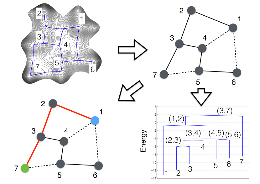
Figure 3. A continuous 7-well potential (top left) is mapped onto a discrete network (top right) by identifying the minimum energy paths (MEPs) connecting the local minima of the potential via saddle points. The states $i$, $j$, … are the indices of these minima, there is an edge between any pair $(i,j)$ if there is a MEP with a single saddle point along it connecting $i$ and $j$. By using the energy of the saddle point $V_{i,j}$ as cost for the edge $(i,j)$, one can find the minimal spanning tree of the network (solid edges in the top right panel) using e.g. Kruskal algorithm, and thereby obtain its disconnectivity graph (bottom right). On this disconnectivity graph, the pairs of numbers at the branching points indicate which of the nodes in the corrsponding bottom parts of the tree connect at that level of energy. Using the Dijkstra-based algorithm proposed in [11] we can also calculated the minmax path connecting two states, for example between states 1 and 7 (solid red path in the bottom left panel). This minmax path is relevant in regimes where LDT applies.

In the set-up above, we can use the temperature $\epsilon$ as control parameter, in such a way that (26) holds when $\epsilon\to 0$. In that limit, for reasons that will become clear below, in general there are as many low-lying groups of eigenvalues as there are states (i.e. $\lambda_{p}/\lambda_{p+1}\to 0$ as $\epsilon\to 0$ for all $p=0,1,\ldots,N-1$), and Wentzell’s approach provides a way to estimate each of these eigenvalues. To see how, it is convenient to organize the states of the chain on a disconnectivity graph, that is, a downward facing tree in which each node $i\in S$ lies at the end of a branch at a depth equal to its energy $V_{i}$, and branches in the tree are connected at the lowest energy barrier $V_{j,k}$ that connect all the nodes on one side of the tree to those on the other side – a cartoon example is shown in Fig. 3: because this will be relevant in our analysis of ${\rm LJ}_{38}$, in this example we start from a continuous energy landscape that we convert into a network whose disconnectivity graph is then obtained from its minimal spanning tree (bottom right, all solid edges) calculated using e.g. Kruskal’s algorithm (see e.g. [1]). The eigenvalues can then be estimated recursively from the disconnectivity graph as follows: Start by identifying the lowest barrier in the tree, i.e. the adjacent pair $(i_{N},j_{N})$ on the tree such that $V_{i_{N},j_{N}}-V_{i_{N}}$ is minimum over all $i,j\in S$. The node $i_{N}$ identifies the well that the system can escape by crossing the barrier of minimum height, and the largest eigenvalue in the system corresponds to the inverse of the time scale of this escape, i.e. it can then be estimated as

(35) $$\lambda_{N-1}\asymp\exp\left(-\frac{1}{\epsilon}(V_{i_{N},j_{N}}-V_{i_{N}})\right)$$

where the symbol $\asymp$ means that the ratio of the logarithms of both sides of this equality tends to 1 as $\epsilon\to 0$. Now remove the node $i_{N}$ and its branch from the tree, and repeat the construction: that is, in the new tree find the pair $(i_{N-1},j_{N-1})$ such that $V_{i_{N-1},j_{N-1}}-V_{i_{N-1}}$ is minimum over all $i,j\in S\setminus\{i_{N}\}$, to obtain an estimate for the next largest eigenvalue, $\lambda_{N-2}$. By iterating upon this procedure, in $N-1$ steps we can then estimate $\lambda_{N-k}$ for $k=2,3,\ldots,N-1$ as

(36) $$\lambda_{N-k}\asymp\exp\left(-\frac{1}{\epsilon}(V_{i_{k},j_{k}}-V_{i_{k}})\right)\qquad\text{where}$$

$$(V_{i_{k},j_{k}}-V_{i_{k}})=\min_{i,j\in S\setminus\{i_{N},i_{N-1},\ldots,i_{N-k+1}\}}(V_{i,j}-V_{i}),$$

Intuitively, this procedure corresponds to lumping together the states that can be be reached on timescales of order $\lambda^{-1}_{k}$ or below, and analyzing what happens on the next timescale to get $\lambda_{k-1}\ll\lambda_{k}$. After $N-1$ steps in the procedure we end up with a degenerate tree made of a single node lying at the very bottom of the original tree (and of course we already know that $\lambda_{0}=0$). Note that in the discussion above, we assumed that the barriers $(V_{i_{k},j_{k}}-V_{i_{k}})$ identified along the way are all different (that is, strictly increasing with $k$), which is the generic case and leads to eigenvalues that are all well-separated: if some of these barriers are equal, it means that some of the eigenvalues are asymptotically equivalent, and this case can be treated as well by generalizing the construction above. Note also that estimates more precise than (35) and (36) can be obtained using the potential theoretic/TPT approach: in the present situation, at any stage in the iteration procedure, the states $i_{k}$ and $j_{k}$ are those that should be set as $A$ and $B$, respectively.

4.3.1. Freidlin’s Cycles and MinMax Paths.

Another interesting construction provided by LDT is the decomposition of the stochastic network into Freidlin’s cycles [19, 20, 21]. For systems satisfying the detailed balance condition and with a rate matrix as in (33), the decomposition into cycles simplifies, as was recently discussed in [11]. Here we summarize this discussion and refer the interested reader to the original paper for details.

In a nutshell, the decomposition into cycles focuses on which states are most likely to be reached from a given state: in the zero temperature limit, if the system is in state $i$, with probability one it will reach next the state connected to $i$ by the smallest barrier, i.e.

(37) $$j_{*}(i)=\mathop{\text{arg min}}\limits_{i\in S}V_{i,j}$$

Searching consecutively for the next most likely state defines a dynamics on the network that generically ends with cycles made of two states: each of these cycles contain a local minimum of energy on the disconnectivity graph (that is, a state at the bottom of a group of branches on the tree), and the state connected to this minimum by the lowest barrier. These cycles are called 1-cycles by Freidlin. Once we have identified them, we can remove from the tree the state with highest energy in each of these 1-cycles, and repeat the construction iteratively. These gives 2-cycles, 3-cycles, etc. until we again end up with a tree with only 2 nodes on it. In this construction, we can also keep the information about the state in the original network by which any $n$-cycle is exited: with probability 1 as $\epsilon\to 0$, this is the state whose barrier is the lowest to escape all the states contained in this $n$-cycle. A corollary of the fact that cycles are exited in a predictable way is that, between any two nodes in the network taken as sets $A$ and $B$, there exists a single path on the network that concentrates all the current of the reactive trajectories as $\epsilon\to 0$. This path has a minmax property: the maximal barrier separating every pair of states $i$ and $j$ on the path is minimal among the maximal barriers along all paths in the network connecting $i$ and $j$ (see Fig. 3 for an illustration).

In [11], the construction of the hierarchy of Freidlin’s cycles was performed via a sequence of conversions of rate matrices into jump matrices followed by taking limits $\epsilon\to 0$. Relying on the properties of the hierarchy of cycles specific for the systems with detailed balance, an efficient Dijkstra-based algorithm was also proposed for computing the minmax path. Importantly, this algorithm did not built the whole hierarchy of cycles, but only computed the sub-hierarchy relevant to the transition process of interest, and did not require any pre-processing of the stochastic network.

We conclude this section on LDT with a remark. As explained above, the LDT picture applies in the limit when $\epsilon\to 0$, in which case the hierarchy of different barriers in the disconnectivity graph corresponds to timescales that become infinitely far apart as $\epsilon\to 0$. While this picture is indeed correct at extremely low temperature, we do not expect it to remain valid as the temperature is increased, even if the system does remain strongly metastable (i.e. such that some low-lying groups of eigenvalue do persist). Rather, we expect that the transition channel will rapidly broaden if the networks is large, and that the mechanism of the reaction wil depart from that predicted by LDT. Our analysis of ${\rm LJ}_{38}$ by TPT will indeed confirm this picture.

5. Application to the Rearrangement of the Lennard-Jones 38 Cluster

5.1. Microscopic Model and Thermodynamic Properties

A Lennard-Jones cluster is made of particles (or atoms) interacting via the Lennard-Jones pairwise potential given by

(38) $$V(r)=4a\sum_{i<j}\left[\left(\frac{\sigma}{r_{ij}}\right)^{12}-\left(\frac{\sigma}{r_{ij}}\right)^{6}\right].$$

Here $r=\{r_{j}\}_{j=1}^{N}\in\mathbb{R}^{3N}$ denotes the positions of the $N$ particles in the cluster, $r_{ij}$ is the distance between particles $i$ and $j$, and $a>0$ and $\sigma>0$ are parameters measuring respectively the strength and range of the interactions. At the most fundamental level, the finite-temperature dynamics of the cluster can be modeled as a continuous diffusion over the potential (38). This dynamics is extremely complicated owing to the multiscale nature of this potential which, when $N$ is large (e.g. $N=38$ as we will consider below) possesses an enormous number of local minima separated by a hierarchy of barriers of various height. A few thermodynamic properties of these clusters are known, however.

First, it is known that the majority of global potential energy minima for Lennard-Jones clusters of various sizes involve an icosahedral packing [38]. However, Lennard-Jones clusters with special numbers of atoms admit a high symmetry configuration based on a face-centered cubic packing, with a lower energy. The smallest cluster with this property contains $N=38$ atoms[16, 35]. The global potential energy minimum of the ${\rm LJ}_{38}$ cluster is achieved by a truncated octahedron with the point group $O_{h}$ (Fig. 1 (a)), which from now on we will simply refer to as FCC. The second lowest minimum is the icosahedral structure with the $C_{5v}$ point group (Fig. 1 (b)), which we will refer to as ICO.

It is also known that the basin around ICO is much wider than that around FCC – these two basins are usually referred to as funnels in the literature. This has thermodynamic consequences when the temperature of the system is non-zero. Indeed, the FCC basin only remains the preferred basin for $T<T_{c}$ with $k_{B}T_{c}\approx 0.12a$ (here $k_{B}$ denotes Boltzmann constant). At $T=T_{c}$, the system undergoes a solid-solid phase transition where the ICO basin becomes more likely due to its with greater configurational entropy (see e.g. Fig. 4 in [35]). Next, at $k_{B}T\approx 0.18a$, the outer layer of the cluster melts, while the core remains solid. Then the cluster completely melts at $k_{B}T\approx 0.35a$ [24].

The difference of widths of the two basins also has dynamical consequences. Indeed, due to its larger width, the ICO basin is the one that is most likely to be reached by the system after crystallization even if $T<T_{c}$. The question then becomes how does the system reorganize itself to get out of the dynamical trap around ICO and in its preferred state around FCC? It is also of interest to understand how this process is influenced by the temperature, since the rearrangement pathway is likely to be influenced by it. These are the type of questions that we will address in this section, as an illustration of the TPT-based network analysis tools presented earlier. This study is complementary to those conducted by Wales and collaborators in the same context [16] using different tools [33, 34, 35, 36].

5.2. Network Representation of the Lennard-Jones 38 Cluster

The problem of rearrangement of ${\rm LJ}_{38}$ has been the object of much studies in the past 15 years (see e.g. [16, 38, 31, 28, 27]). An interesting approach to the problem has been proposed by David Wales and collaborators, who undertook an ambitious program aiming at mapping the evolution of ${\rm LJ}_{38}$ onto a network/MJP and reducing the analysis of the dynamics of ${\rm LJ}_{38}$ to the study of this network. While this mapping is technically hard to perform in practice and required a lot of inventiveness, it is conceptually quite simple to understand. If the temperature of the system is small enough, it will spend a long time near the bottom of the energy well around the local minima it is currently in before a thermal fluctuation large enough will manage to push it above an energy barrier separating it from an adjacent well. The system will then fall near the bottom of this adjacent well and the process will repeat. In this regime, the dynamics can be reduced to a basin hoping: the local minima of the energy become the nodes on the network, two such nodes are connected by an edge if the system can transit from one minimum to the another by crossing a single barrier, and the rate/weight of the directed edge from one node to another involves (via Arhennius formula) the height of the energy barrier(s) that must be crossed to perform this transition – this construction was illustrated on a toy example in Fig. 3. An additional simplification made in the case of ${\rm LJ}_{38}$ is to lump together all the minima and saddle point that are equivalent by symmetry (point group, permutation, etc.). All together this construction led to a network for ${\rm LJ}_{38}$ that contains a single connected component with 71887 nodes associated with the lowest local minima on the landscape (which include FCC and ICO), and 119853 edges – this information is publicly available from the ${\rm LJ}_{38}$ database Wales’s website [37]. The database also contains the information about the generator, whose off-diagonal entries are in a form consistent with (33) [34]

(39) $$L_{i,j}=\sum_{k}\frac{O_{i}\bar{\nu}_{i}^{\kappa}}{O^{k}_{i,j}(\bar{\nu}^{k}_{i,j})^{\kappa-1}}e^{-\beta(V^{k}_{i,j}-V_{i})}$$

Here $\beta=1/k_{B}T$ is proportional to the inverse of the system’s temperature $T$, $O_{i}$, $V_{i}$, and $\bar{\nu}_{i}$ are, respectively, the point group order, the value of the potential energy, and the geometric mean vibrational frequency for the local minimum associated with node $i$, $O^{k}_{i,j}=O^{k}_{j,i}$, $V^{k}_{i,j}=V^{k}_{j,i}$ and $\bar{\nu}^{k}_{i,j}=\bar{\nu}^{k}_{j,i}$ are the same numbers for the transition state $k$ connecting the local minima $i$ and $j$ (there may be more than one of them for every pair $(i,j)$ adjacent on the network), and $\kappa=3\times 38-6=108$ is the number of vibrational degrees of freedom. As in (33), if there is no minimum energy path connecting the minima with index $i$ and $j$ via a single saddle point, we set $k=1$ and $V^{1}_{i,j}=\infty$. Note that, by construction, the generator defined by (39) satisfies detailed-balance with respect to the following Boltzmann-Gibbs equilibrium distribution:

(40) $$\pi_{i}=\frac{1}{Z(\beta)}\frac{e^{-\beta V_{i}}}{O_{i}\bar{\nu}_{i}^{\kappa}}\qquad\qquad Z(\beta)=\sum_{i\in S}\frac{e^{-\beta V_{i}}}{O_{i}\bar{\nu}_{i}^{\kappa}}.$$

The network representation of ${\rm LJ}_{38}$ via (39) will be our starting point here. The majority of local minima/nodes listed in Wales database do not have special names – for example, FCC and ICO are simply listed 1st and 7th, respectively. Except for these two, in the sequel we will simply refer to the other minima by their indices in the database. We also work in reduced units in which the temperature is measured in units of $a/k_{B}$. Since we are interested in the mechanism of rearrangement between ICO and FCC, we take the nodes of these two states as sets $A$ and $B$, respectively. We also checked that our results do not change significantly if we fatten these states by including in them the nodes that are in the connected component around them where all the nodes have energy within $k_{B}T$ of that of FCC and ICO, respectively.

5.3. Computational Aspects of the TPT Analysis of ${\rm LJ}_{38}$

A key preliminary step in the application of TPT to ${\rm LJ}_{38}$ is the calculation of the committor function. This calculation requires solving (6) which, in the present case, is a system of $71887-2=71885$ linear equations with the same number of unknowns. The detailed balance property (3) allows us to make the matrix in (6) symmetric by multiplying each row by $(O_{i}\bar{\nu}_{i}^{\kappa})^{-1}e^{-\beta V_{i}}$. The resulting system can then be solved using the conjugate gradient method with the incomplete Cholesky preconditioning (see e.g. [29]). This works for $T\geq 0.125$. For lower values of the temperature, the scale separation between the possible values of $e^{-\beta V_{i}}$ for different $i$ becomes too large for the computer arithmetics. In order to overcome this difficulty we truncate the ${\rm LJ}_{38}$ network by keeping only the nodes whose energy is below a given cap – this is legitimate because, the lower the temperature, the least likely it is to observe a reactive trajectory venturing at energies much higher than $k_{B}T$ above that of the overall barrier between ICO and FCC. For each value of temperature we set this cap as high as possible while keeping the system nonsingular in the computer arithmetics. The energy caps and resulting network sizes for the different values of temperature that we considered are listed in Table 1. The values in parentheses are the difference between the caping energy and that of FCC, $V_{{\rm FCC}}=-173.928$ [37]. All in all, we computed the committor for temperatures ranging from $T=0.04$ to $T=0.18$ using steps of $\Delta T=0.005$.

The disconnectivity graphs of the network we used at three different temperatures, $T=0.06$, $T=0.12$, and $T=0.15$ are shown in Fig. 4. On these figures, we only included the nodes through which at $1\%$ of the total current of reactive trajectories goes and we colored the branches of the graph according to the value of the committor of the nodes at the end of these branches. As can be seen, as the temperature increases, the committor function becomes less step-like, and a higher number of nodes gets values than are in between the extreme 0 and 1.

Table 1. Energy caps and network sizes used for different value of the temperature.

Temperature $T$	Energy cap	Number of states
0.04 $\leq T\leq$ 0.05	-169.5 (4.428)	1604
0.055	-168.5 (5.428)	15056
0.06, 0.065	-168.0 (5.928)	28486
0.07	-167.0 (6.928)	53566
0.075, 0.08	-166.5 (7.428)	61706
0.085	-165.5 (8.428)	69302
0.09, 0.095	-165.0 (8.928)	70552
0.10 $\leq T\leq$ 0.12	-164.0 (9.928)	71609
0.125 $\leq T\leq 0.18$	$\infty$	71887

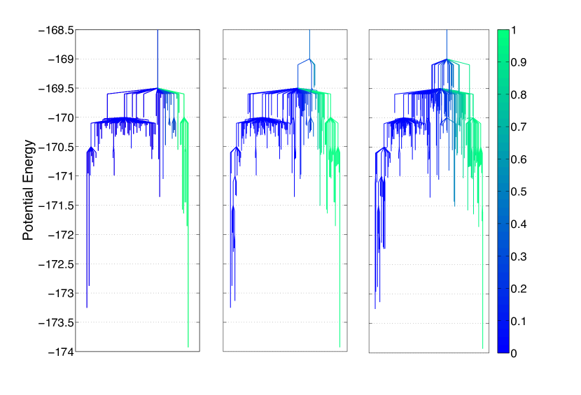
Figure 4. Disconnectivity graphs colored according to the value of the committor: $T=0.06$ (left), $T=0.12$ (center), $T=0.15$ (right). Each disconnectivity graph includes only those local minima through which at least 1% of the reaction pathways from ICO to FCC pass.

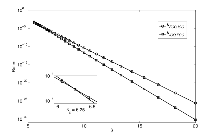
Figure 5. The reaction rates in (13) computed with $A=$ ICO and $B=$ FCC at different temperatures. These rates display an almost perfect Arrhenius-like behavior in this temperature range, even though the mechanism of the rearrangement becomes increasingly complex as the temperature increases. The zoom shown in the inset shows that a cross-over between $k_{\text{FCC,ICO}}$ and $k_{\text{ICO,FCC}}$ occurs ar $\beta_{c}=6.25$ (i.e. $T_{c}=0.16$): this is the temperature above which ICO becomes more favorable than FCC due to entropic effects related to the relative widths of the funnels around these two structures.

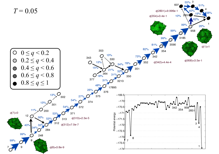
Figure 6. Cartoon representation of the network of current of reactive trajectories at $T=0.05$. The edges shown carry at least 10% of the total reactive flux from ICO to FCC – the thickness of the arrow is proportional to the precentage of current the edge carries, and the actual percentage is also displayed next to it. The values of the committor at the nodes are show in greyscale, with the explicit values of $q$ given for some of them. The blue arrows show the minmax path from LDT: at this low temperature, most of the current goes along this path. The highest barrier crossed along the minmax path is between nodes $342$ and $254$ ($V_{(342,254)}=4.219$). Also show in inset is the energy profile along the minmax path.

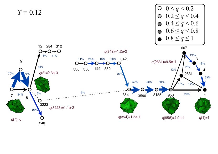
Figure 7. Same as in Fig. 6 at $T=0.12$. At this higher temperature, most of the edges carry less than $10\%$ of the total current: in particular, we can no longer go from ICO to FCC by following edges that carry at least $10\%$ of the current. This also implies that the minmax path from LDT is no longer relevant to explain the mechanism of the rearrangement at this temperature – the edges along this path that carry more than $10\%$ of the current are still shown in blue. The edges between nodes 8 and 3223 and nodes 3223 and 354 carry less than $5\%$ of the current: we show them because these edges belong to the dominant representative path introduced, i.e. the path maximizes the current it carries. This path is different from the minmax path but, as can be seen in this example, it is not relevant either in situations where the transition channel becomes spread out.

Figure 8. Empirical cumulative distribution function of the highest energy barrier along the no-detour paths at different temperature. The height of the barriers are given respective to the energy of FCC, $V_{\text{FCC}}=−173.928$. As the temperature increases, the no-detour paths tend to cross higher barriers.

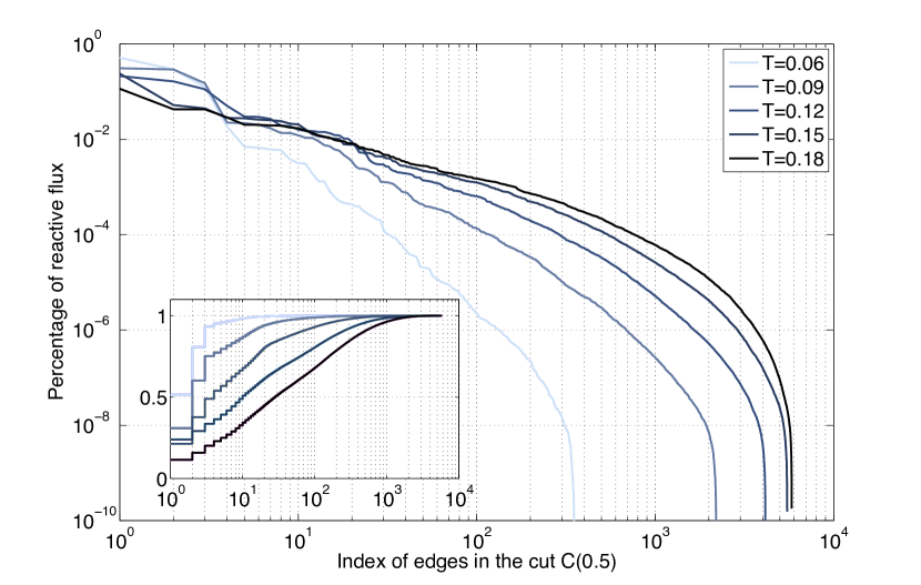
Figure 9. The magnitude of the current through the edges in the isocommittor cut $C(0.5)$ is plotted against the index of these edges ordered by this magnitude. The inset shows the empirical cumulative distribution function of the current through the edges in the cut. The number of edges that must be included to account for a given percentage of the total current increases rapidly with temperature, indicative of the broadening of the reaction channel for the rearrangement.

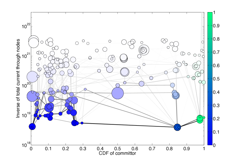
Figure 10. Graphical representation of the network of reactive current in ${\rm LJ}_{38}$ at $T=0.06$. The way this representation was constructed is explained in text.

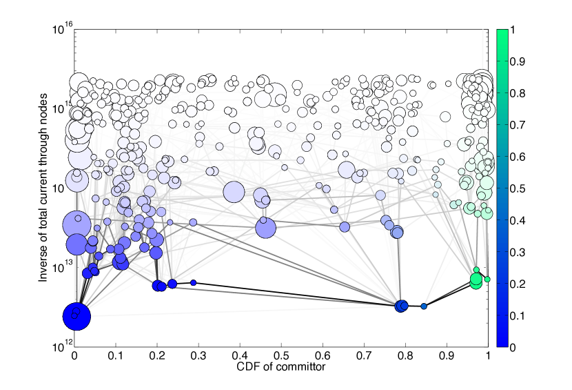
Figure 11. Same as in Fig. 10 at $T=0.09$.

Figure 12. Same as in Fig. 10 at $T=0.12$.

Figure 13. Same as in Fig. 10 at $T=0.15$.

5.4. Rate and Mechanism of Rearrangement at Different Temperatures

Once the committor function has been calculated, we can use TPT to calculate the rate of rearrangement of ${\rm LJ}_{38}$ and characterize its mechanism. Using formulae (13) with $A=$ ICO and $B=$ FCC, we obtain the rates at which the system rearranges itself between these two states. These rates are shown in Fig. 5 as a function of the inverse temperature $\beta$. As can be seen, both rates are almost perfectly straight on a log-linear scale, and can be fitted by

(41) $$k_{\text{FCC,ICO}}=1.03\times 10^{7}e^{-4.289\beta},\qquad k_{\text{ICO,FCC}}=9.81\times 10^{4}e^{-3.525\beta}$$

Since the energy barriers between FCC and ICO and ICO and FCC are 4.219 and 3.543, respectively, [16], these fits are consistent with Arrhenius law. The fits in (41) also compare well with the ones calculated in [35] for the temperature range $0.03\leq T\leq 0.4$: $k_{\text{FCC,ICO}}=2.13\times 10^{6}e^{-4.29\beta}$ and $k_{\text{ICO,FCC}}=1.16\times 10^{3}e^{-3.43\beta}$. Note also that the rates cross at the value $\beta=6.25$ (i.e. $T=0.16$): this temperature is the one above which TPT predicts that ICO becomes preferred over FCC, which is slightly higher than the value $T_{c}=0.12$ listed in Sec. 5.1. This crossover is due to entropic effects related to the relative widths of the funnels around ICO and FCC.

The Arrhenius-like nature of the rates may suggest that the mechanism of rearrangement of the ${\rm LJ}_{38}$ cluster is quite simple, and dominated at all the temperatures that we considered by the hoping over the lowest saddle point separating ICO and FCC. This impression, however, is deceptive. To see why, in Figs. 6 and 7 let us compare cartoon representations of the current of reactive trajectories given in (10) at two different temperatures, $T=0.05$ and $T=0.12$. The way these representations were constructed is by plotting all the nodes in the network such that the current of reactive trajectories along the edges between them carry at least 10$\%$ of the total current, and connecting these nodes by an arrow whose thickness is proportional to the magnitude of the current. As can be seen in Fig. 6, at $T=0.05$, most of the current concentrate on a single path: this path coincides with the minmax path between ICO and FCC predicted by LDT [11]. At the higher temperature of $T=0.12$, however, we see that this minmax path becomes mostly irrelevant, and in fact we can no longer go from ICO to FCC following edges that carry at least 10$\%$ of the current. The reason is that the current becomes very spread out among the edges of the network, indicative that the tube carrying most of the current of reactive trajectories also becomes quite wide.

To quantify further this observation, we used Proposition 2 to generate $10^{8}$ samples of the no-detour transition path process at every temperature. (In the present example, it turns out that the network is so complex that the reactive trajectories themselves, which we can in principle generate via Proposition 1, are too long to be sampled efficiently. This arises because these trajectories wander too often into quasi-deadends or in between intermediate structures, and this is why we focused on no-detour transition paths which are much shorter and can be generated in great number.) We used this sample of no-detour transition paths to first analyze the height of the highest energy barrier along these paths measured with respect to $V_{\text{FCC}}=-173.928$. The empirical cumulative distribution functions of these barrier heights are shown in Fig. 8. As can be seen, at the low temperature of $T=0.05$, this distribution is very peaked around the value $4.219$, which is the height of the lowest saddle point separating ICO and FCC. At higher temperatures, however, this distribution broadens significantly, indicative that higher barriers become frequently crossed by the no-detour transition paths. This is an entropic effect: in essence, we can think of the height of the barrier in terms of ‘bonds’ between the Lennard-Jones particles that need to be broken for the rearrangement to proceed. What our results show is that the number of no-detour paths increases very rapidly with the maximal number of bonds that are ever broken along them. At low temperature, the rearrangement proceed mostly by no-detour paths along which no more than about 4 bounds are broken, because these paths are energetically favorable. At higher temperature, however, no-detour paths along which 5, 6 or even 7 bonds break start to matter: even though they are less favorable energetically, their sheer number means that they eventually carry more current globally.

A consequence of this effect is that the width of the reaction channel also broadens significantly with temperature. This is quantified in Fig. 9, where we analyze the current along the edges in the isocommittor cut $C(0.5)$. By ordering these edges by the magnitude of the current they carry, and plotting this current magnitude as a function of the edge index, we arrive at the plots on the main panel of Fig. 9. As can be seen, as the temperature increases, these plots widen with temperature, and display a power law behavior for a range of edge indices. The inset of Fig. 9 shows the cumulative distribution of the current through the edges in the isocommittor cut $C(0.5)$, and show that the higher the temperature, the more edges need to be included to get a significant percentage of the total current: for example, at $T=0.18$, thousands of edges in the cut (that is, most of them) need to be included in order to account for $95\%$ of the current. The mechanism of rearrangement thus departs significantly from the one predicted by LDT, even though the rates remain Arrhenius-like even at this high temperature.

We tried to capture visually the complexity of the mechanism of rearrangement using the representation of the network of current of reactive trajectories shown in Figs. 10–13. These figures were constructed as follows. We plotted every node of the network through which at least $0.1\%$ of the total current went. We ordered these nodes along the $x$-axis according to the cumulative distribution function of their committor, using a coloring from blue to green to indicate their actual committor value. Along the $y$-axis, we ordered the nodes according to the inverse of the magnitude of current of reactive trajectory, (10), they carry (the higher the node, the least current it carries) and we connected the nodes by lines whose darkness is proportional to the magnitude of the current between them. We also faded the color as this magnitude decreased. Finally, we used dots of different sizes to represent the nodes: the bigger the node, the larger is the magnitude of the average number of transitions per unit time that the reactive trajectories make through this node, see (9). This is a way to try to capture deadends and dynamical traps on the network, i.e. node that the reactive trajectories visit often but through which little current of these reactive trajectories go. In the figures these deadends are nodes that are high and big. Overall, what these figures confirm is that, as the temperature increases, the curent of reactive trajectories spreads more and more on the network, and the reaction channel broadens. It also confirms that there exists many deadends and dynamical traps on the network. This last aspect makes TPT particularly suitable to analyze the mechanism of rearrangement: indeed, a spectral analysis of the network along the lines discussed in Sec. 4.1 is both hard to perform in the present situation and uninformative because it is too global.

6. Outlook and Conclusions

We have presented a set of analytical and computational tools based on TPT to analyze flows on complex networks/MJPs. We expect these tools to be useful in a wide variety of contexts. The network representation of ${\rm LJ}_{38}$ that we used here as illustration is just a specific example of Markov State Model (MSM) used to map a complex dynamical system onto a MJP (see e.g. [10]). During the last decade, such MSMs have emerged as a way to analyze timeseries data generated e.g. by molecular dynamics simulations of macromolecules, general circulation models of the atmosphere/ocean system, etc. In these contexts, massively parallel simulations, special-purpose supercomputers, and high-performance graphic processing units (GPUs) permit to generate time series data in amounts too large to be grasped by traditional “look and see” techniques. MSMs provide a way to analyze these data by partitioning the conformation space of the molecular system into discrete substates, and reducing the original kinetics of the system to Markov jumps between these states – in other words, by interpreting the timeseries as some dynamics on a network, with the states in the MSMs playing the role of the nodes on the network, and the transition rates between these states being the weights of the directed edges between these nodes. While MSMs typically provide an enormous simplification of the original timeseries data, the associated networks are typically quite complex themselves, with many nodes, a nontrivial topology of edges between them, and rates/weights on these edges that can span a wide range of scales. The tools that we derived from TPT can be used for the nontrivial task of analyzing these networks/MSMs.

More generally, we expect the tools developed in this paper to be useful to analyze and interpret other networks that have emerged in many areas as a way to represent complex data sets.

References

- [1] Ahuja, R. K., Magnanti, T. L, Orlin, J. B.: Network flows: Theory, Algorithms, and Applications. Prentice Hall (1993).
- [2] Beltrán, J., Landim, C.: Tunneling and metastability of continuous time Markov chains. J. Stat. Phys. 140, 1065-–1114, (2010).
- [3] Berezhkovskii, A., Hummer, G., Szabo, A.: Reactive flux and folding pathways in network models of coarse-grained protein dynamics. J. Chem. Phys. 130, 205102 (2009).
- [4] Berman, K. A., Konsowa, M. H.’: Random paths and cuts, electrical networks, and reversible Markov chains. SIAM J. Discrete Math. 3, 311–-319 (1990).
- [5] Bianchi, A., Bovier, A., Ioffe, D.: Sharp asymptotics for metastability in the random field Curie-Weiss model. Electron. J. Probab. 14, 1541-1603 (2009).
- [6] Bovier, A.: Metastability. In Methods of Contemporary Statistical Mechanics. R. Kotecky, Ed., LNM 1970, Springer, Berlin (2009).
- [7] Bovier, A., Eckhoff, M., Gayrard, V. Klein, M.: Metastability and Low Lying Spectra in Reversible Markov Chains. Commun. Math. Phys. 228, 219–255 (2002).
- [8] Bovier, A., Eckhoff, M., Gayrard, V. Klein, M.: Metastability in reversible diffusion processes 1. Sharp estimates for capacities and exit times. J. Eur. Math. Soc. 6, 399–424 (2004).
- [9] Bovier, A., Gayrard, V., Klein, M.: Metastability in reversible diffusion processes. 2. Precise estimates for small eigenvalues. J. Eur. Math. Soc. 7, 69–99 (2005).
- [10] Bowman, G. R., Pande, V. S., and Noé, F. eds.: An Introduction to Markov State Models and Their Application to Long Timescale Molecular Simulation. Advances in Experimental Medicine and Biology, 797. Springer (2014).
- [11] Cameron, M. K.: Computing Freidlin’s cycles for the overdamped Langevin dynamics. J. Stat. Phys, 152, 493–518 (2013).
- [12] Den Hollander, F.: Three lectures on metastability under stochastic dynamics. In Methods of Contemporary Mathematical Statistical Physics (R. Kotecky, ed.). Lecture Notes in Math. 1970. Springer, Berlin. (2009).
- [13] Den Hollander, F., Jansen, S.: Berman-Konsowa principle for reversible Markov jump processes. arXiv:1309.1305v1
- [14] Dijkstra, E. W.: A Note on Two Problems in Connexion with Graphs. Numerische Mathematic, 1, 269–271 (1959).
- [15] Doyle, P. G., Snell, J. L.: Random Walks and Electric Networks, volume 22 of Carus Mathematical Monographs. Mathematical Association of America, Washington, DC (1984).
- [16] Doye, J. P. K., Miller, M. A., Wales, D. J.: The double-funnel energy landscape of the 38-atom Lennard-Jones cluster. J. Chem. Phys. 110, 6896–6906 (1999).
- [17] E, W., Vanden-Eijnden, E.: Toward a Theory of Transitions Paths. J. Stat. Phys. 123, 503–523 (2006).
- [18] E, W., Vanden-Eijnden, E.: TRansition-Path Theory and Path-Finding Algorithms for the Study of Rare Events. Ann. Rev. Phys. Chem. 61, 391–420 (2010).
- [19] Freidlin, M. I.: Sublimiting distributions and stabilization of solutions of parabolic equations with small parameter. Soviet Math. Dokl. 18(4), 1114–1118 (1977).
- [20] Freidlin, M. I., Wentzell, A. D.: Random Perturbations of Dynamical Systems. 3rd ed., Springer-Verlag, Berlin, Heidelberg (2012).
- [21] Freidlin, M. I.: Quasi-deterministic approximation, metastability and stochastic resonance. Physica D, 137:333–352 (2000).
- [22] Landim, C.: A topology for limits of Markov chains. arXiv:1310.3646
- [23] Lu, J., Nolen, J.: Reactive trajectories and transition path processes. arXiv:1303.1744
- [24] Mandelshtam, V. A., Frantsuzov, P. A.: Multiple structural transformations in Lennard-Jones clusters: Generic versus size-specific behavior. J. Chem. Phys. 124, 204511 (2006).
- [25] Metzner, P., Schuette, Ch., Vanden-Eijnden, E.: Illustration of transition path theory on a collection of simple examples. J. Chem. Phys. 125, 084110 (2006).
- [26] Metzner, P., Schuette, Ch., and Vanden-Eijnden, E.: Transition path theory for Markov jump processes. SIAM Multiscale Model. Simul. 7, 1192–1219 (2009).
- [27] Miller III, T. F., Predescu, C.: Sampling diffusive transition paths. J. Chem. Phys. 126, 144102 (2007).
- [28] Neirotti, J. P., Calvo, F., Freeman, D. L., Doll, J. D.: Phase changes in 38-atom Lennard-Jones clusters. I. A parallel tempering study in the canonical ensemble. J. Chem. Phys. 112, 10340 (2000).
- [29] Nocedal, J., Wright, S. J.: Numerical Optimization. 2nd Ed. Springer Series in Operational Research. Springer Verlag. (2006).
- [30] Olivieri, E., Vares, M. E. Large deviations and metastability. Encyclopedia of Mathematics and its Applications, vol. 100. Cambridge University Press, Cambridge (2005).
- [31] Picciani, M., Athenes, M., Kurchan, J., Taileur, J.: Simulating structural transitions by direct transition current sampling: The example of . J. Chem. Phys., 135, 034108 (2011).
- [32] Vanden-Eijnden E.:Transition path theory. In Computer Simulations in Condensed Matter: From Materials to Chemical Biology. Vol. 1, ed. M Ferrario, G Ciccotti, K Binder, pages 439–-78. Springer, Berlin (2006).
- [33] Wales, D. J.: Discrete Path Sampling. Mol. Phys., 100, 3285–3306 (2002).
- [34] Wales, D. J.: Some further applications of discrete path sampling to cluster isomerization. Mol. Phys., 102, 891–908 (2004).
- [35] Wales, D. J.: Energy landscapes: calculating pathways and rates. International Review in Chemical Physics 25, 237–282 (2006).
- [36] Wales, D.J.: Calculating Rate Constants and Committor Probabilities for Transition Networks by Graph Transformation. J. Chem. Phys. 130, 204111 (2009).
- [37] Wales’s website contains the database for the Lennard-Jones-38 cluster: http://www-wales.ch.cam.ac.uk/examples/PATHSAMPLE/
- [38] Wales, D. J., Doye, J. P. K.: Global Optimization by Basin-Hopping and the Lowest Energy Structures of Lennard-Jones Clusters containing up to 110 Atoms. J. Phys. Chem. A 101, 5111–5116 (1997).
- [39] Wentzell, A. D.: On the asymptotics of eigenvalues of matrices with elements of order . Soviet Math. Dokl., 13, 65–68 (1972).