Abstract

Consider a smooth vector field $f\colon\mathbb{R}^{n}\to\mathbb{R}^{n}$ and a maximal solution $\gamma\colon\,]a,b[\,\to\mathbb{R}^{n}$ to the ordinary differential equation $x^{\prime}=f(x)$. It is a well-known fact that, if $\gamma$ is bounded, then $\gamma$ is a global solution, i.e., $\,]a,b[\,=\mathbb{R}$. We show by example that this conclusion becomes invalid if $\mathbb{R}^{n}$ is replaced with an infinite-dimensional Banach space.

Classification: Primary 34C11; secondary 26E20, 34A12, 34G20, 37C10, 34–01
Key words: Ordinary differential equation, smooth dynamical system, autonomous system, Banach space, finite life time, maximal solution, bounded solution, relatively compact set, tubular neighborhood, nearest point
Introduction and statement of result
The starting point for our journey is a well-known result in the theory of ordinary differential equations: If the image $\gamma(]a,b[)$ of a maximal solution $\gamma\colon\,]a,b[\,\to U$ to a differential equation

$$x^{\prime}=f(x)$$

with locally Lipschitz right-hand side $f\colon U\to\mathbb{R}^{n}$ on an open subset $U\subseteq\mathbb{R}^{n}$ is relatively compact in $U$, then $\gamma$ is globally defined, i.e., $]a,b[\,=\mathbb{R}$ (cf. [7, Chapter I, Theorem 2.1], [9, Korollar in 4.2.III], [11, Corollary 2 in §2.4]). In the special case $U=\mathbb{R}^{n}$, this entails that bounded maximal solutions $\gamma\colon\,]a,b[\,\to\mathbb{R}^{n}$ are always globally defined, exploiting that bounded sets and relatively compact subsets in $\mathbb{R}^{n}$ coincide by the Theorem of Bolzano-Weierstrass (see, e.g., Corollaire 1 in [1, Chapter IV, §1, no. 5], or [12, Lemma 2.4] for this fact).
The first criterion applies equally well if $\mathbb{R}^{n}$ is replaced with a Banach space (cf. [10, Chapter IV, Corollary 1.8]). However, bounded maximal solutions to ordinary differential equations in infinite-dimensional Banach spaces need not be globally defined. Non-autonomous examples with locally Lipschitz right hand sides were given in [5] (in the Banach space $c_{0}$) and for Banach spaces admitting a Schauder basis in [3], [4]. By now, it is known that the pathology occurs for suitable autonomous systems on every infinite-dimensional Banach space, with locally Lipschitz right-hand side [8].
In the current note, we describe an easy, instructive example of a non-global, bounded solution to a vector field on a separable Hilbert space. In contrast to all of the cited literature, the vector field we construct is not only locally Lipschitz, but smooth (i.e., $C^{\infty}$).
Theorem. There exists a smooth vector field $f\colon\mathcal{H}\to\mathcal{H}$ on the real Hilbert space $\mathcal{H}:=\ell^{2}(\mathbb{Z})$ of square summable real sequences $(a_{n})_{n\in\mathbb{Z}}$, such that the ordinary differential equation $x^{\prime}=f(x)$ has a bounded maximal solution $\gamma$ which is not globally defined.
Our strategy is to describe, in a first step, a smooth curve $\gamma\colon\,]{-1},1[\,\to\mathcal{H}$ whose restrictions to $\,]{-1},0]$ and $[0,1[$ have infinite arc length (Section 1). In a second step, we construct a smooth vector field $f\colon\mathcal{H}\to\mathcal{H}$ such that

$$\gamma^{\prime}(t)=f(\gamma(t))\quad\mbox{for all~{}$\,t\in\,]{-1},1[$,}$$

ensuring that $\gamma$ is a solution to $x^{\prime}=f(x)$ (Section 2). Thus $\gamma$ is not globally defined and it has to be a maximal solution because otherwise the arc length on one of the subintervals would be finite (contradiction).

1 The long and winding road

We fix a function $h\colon\mathbb{R}\longrightarrow\mathbb{R}$ with the following properties:

• $h$ is smooth ($C^{\infty}$) with compact support inside $[-2,1]$;

• $h(-2)=h(-1)=h(1)=0$;

• $h(0)=1$;

• $h^{\prime}(t)>0$ for all $t\in[-1,0[$, $h^{\prime}(t)<0$ for $t\in\,]0,1[$ (whence $h(t)>0$ there) and $h^{\prime}(0)=0$.

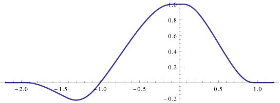
Figure 1: Graph of the function $h$

The existence of such a function is shown in Section 3.
Using this function, we can define a smooth curve with values in the Hilbert space $\mathcal{H}=\ell^{2}(\mathbb{Z})$ via

$$\eta\colon\mathbb{R}\to\mathcal{H},\quad t\mapsto\sum_{k\in\mathbb{Z}}h(t-k)e_{k},\vspace{-2mm}$$

where $\left(e_{k}\right)_{k\in\mathbb{Z}}$ denotes the standard orthonormal basis of $\mathcal{H}$. Note that this sum is locally finite since $h$ has compact support; hence $\eta$ is smooth.

Figure 2: The curve $\eta$ on the interval $[0,1]$

Calculating the derivative $\eta^{\prime}(t)=\sum_{k\in\mathbb{Z}}h^{\prime}(t-k)e_{k}$, we see that $\eta^{\prime}(t)$ is always non-zero. In fact, if $n\in\mathbb{Z}$ with $t\in[n,n+1[$, then $t-n-1\in[{-1},0[$ and thus $\langle e_{n+1},\eta^{\prime}(t)\rangle=h^{\prime}(t-n-1)\not=0$.
By construction of $\eta$, we have $\eta(n)=e_{n}$ for each $n\in\mathbb{Z}$, which implies that $\eta$ has infinite arc length. Since the real-valued function $h$ is bounded, it follows that the curve $\eta$ is (norm-) bounded in the Hilbert space $\mathcal{H}$.
Next, we fix a diffeomorphism $\varphi\colon]{-1},1[\,\longrightarrow\mathbb{R}$ between the open interval $]{-1},1[$ and the real line, e.g. $\varphi(t)=\tan(\frac{\pi}{2}t)$ or $\varphi(t)=\frac{t}{1-t^{2}}$. We now define

$$\gamma\colon]{-1},1[\,\to\mathcal{H},\quad t\mapsto\eta(\varphi(t)).$$

This curve is just a reparametrization of $\eta$ and hence shares some important properties with $\eta$, namely it is bounded in $\mathcal{H}$, the derivative is always nonzero and it has infinite arc length. However, one important difference is that $\gamma$ is not globally defined, so if we are able to show that $\gamma$ is a maximal solution to a (time-independent) differential equation, then our theorem is established.

2 The surrounding landscape

Having constructed the curve $\gamma\colon]{-1},1[\,\longrightarrow\mathcal{H}$ in Section 1, we shall now define a smooth vector field $f\colon\mathcal{H}\longrightarrow\mathcal{H}$ such that $\gamma$ is a solution to the differential equation $x^{\prime}=f(x)$. Since $\gamma$ (as well as its restriction to $]{-1},0]$ and its restriction to $[0,1[$) has infinite arc length by construction, the solution is maximal, and our theorem follows.
Write $\langle x,y\rangle:=\sum_{n\in\mathbb{Z}}x_{n}y_{n}$ for $x=(x_{n})_{n\in\mathbb{Z}}$, $y=(y_{n})_{n\in\mathbb{Z}}$ in $\mathcal{H}$, and $\|x\|:=\sqrt{\langle x,x\rangle}$. We shall use the following facts about distances (to be proven in Section 4):

• The distance function

  $$d_{\gamma}\colon\mathcal{H}\to\,[0,\infty[,\quad x\mapsto\inf\big{\{}\left\|\gamma(t)-x\right\|\colon t\in\,]{-1},1[\big{\}}$$

  from the curve $\gamma$ is continuous on $\mathcal{H}$. In particular, the set $U_{r}:=\left\{x\in\mathcal{H}\colon d_{\gamma}(x)<r\right\}$ is open and contains the image of $\gamma$, for each $r>0$.

• There is a number $\rho>0$ such that for all $x\in U_{\rho}$ there exists a unique $\tau(x)\in\,]{-1},1[$ such that $\gamma(\tau(x))$ has minimum distance to $x$, that is $\left\|\gamma(\tau(x))-x\right\|=d_{\gamma}(x)$.

• The map $\tau\colon U_{\rho}\longrightarrow\,]{-1},1[$ is smooth.

The preceding properties entail that the squared distance function

$$d_{\gamma}^{2}\colon U_{\rho}\longrightarrow[0,\infty[\colon x\mapsto(d_{\gamma}(x))^{2}=\left\|\gamma(\tau(x))-x\right\|^{2}$$

is smooth on the neighborhood $U_{\rho}$ of $\gamma$. This enables us to define the smooth vector field $f$, using a suitable cut-off function $\theta$:

$$f\colon\mathcal{H}\to\mathcal{H},\quad x\mapsto\left\{\begin{array}[]{cl}\theta\left(d_{\gamma}^{2}(x)\right)\gamma^{\prime}(\tau(x))&\mbox{if $\,d_{\gamma}(x)<\rho$;}\\ 0&\mbox{if $\,d_{\gamma}(x)>\rho/2$.}\end{array}\right.$$

Here, $\theta\colon\mathbb{R}\longrightarrow\mathbb{R}$ is a fixed smooth function with $\theta(0)=1$ which vanishes outside of $[{-\rho^{2}/4},\rho^{2}/4]$. It is easily checked using the properties (a), (b) and (c) that the map $f$ is well defined and smooth. The curve $\gamma$ is a solution to the associated differential equation, since for all $t\in\,]{-1},1[\,$:

$$f(\gamma(t))=\theta\Big{(}\underbrace{d_{\gamma}^{2}(\gamma(t))}_{=0}\Big{)}\,\gamma^{\prime}(\ \underbrace{\tau(\gamma(t))}_{=t}\ )=\gamma^{\prime}(t).\vspace{-2mm}$$

This shows that there is a smooth vector field $f$ on $\mathcal{H}$ such that a maximal solution of the differential equation is bounded but has only finite lifetime.

3 Details for Section 1

In Section 1, we used a function $h\colon\mathbb{R}\to\mathbb{R}$ with certain properties (i)–(iv).We now prove the existence of $h$. By the Fundamental Theorem,

$$h\colon\mathbb{R}\longrightarrow\mathbb{R}\colon x\mapsto\int_{-2}^{x}\!g(t)\,dt$$

with a suitable smooth function $g\colon\mathbb{R}\longrightarrow\mathbb{R}$. This reduces the problem of finding $h$ to the problem of finding a function $g$ with the following properties:

• $g$ is smooth with support inside $[{-2},1]$ and integral $\int_{-2}^{1}g(t)dt=0$;

• $\int_{-2}^{-1}g(t)dt=0$;

• $\int_{-1}^{0}g(t)dt=1$;

• $g(t)>0$ for all $t\in[{-1},0[\,$, $g(t)<0$ for all $t\in\,]0,1[\,$, and $g(0)=0$.

It remains to construct such a function $g$. To this end, we start with a smooth function $\psi\colon\mathbb{R}\longrightarrow\mathbb{R}$ which is positive on $]{-1},1[$ and zero elsewhere, e.g.

$$\psi\colon\mathbb{R}\longrightarrow\mathbb{R}\colon t\mapsto\left\{\begin{array}[]{r l}e^{-\frac{1}{1-t^{2}}}&\ \mathrm{if}\ \left|t\right|<1\\ 0&\ \mathrm{else.}\end{array}\right.$$

Using dilations and translations, we can create a function $\psi_{]a,b[}$ from the preceding one, which is positive on any given interval $]a,b[\,$:

$$\psi_{]a,b[}\colon\mathbb{R}\longrightarrow\mathbb{R}\colon t\mapsto\psi\left({-1}+2\,\frac{t-a}{b-a}\right).$$

Now, we define the function $g$ as

$$g:=A\cdot\psi_{]-2,-1[}+B\cdot\psi_{]-3/2,0[}+C\cdot\psi_{]0,1[}$$ (1)

with constants $A,B,C\in\mathbb{R}$ determined as follows:
Condition (iii)^′ requires that $B=(\int_{-1}^{0}\psi_{]{-3/2},0[}(t)\,dt)^{-1}$. Thus $B>0$.
Condition (ii)^′ requires that $A\int_{-2}^{-1}\psi_{]{-2},{-1}[}(t)\,dt=-B\int_{-3/2}^{-1}\psi_{]{-3/2},0[}(t)\,dt$ with $B$ as just determined. This equation can uniquely be solved for $A$ (with $A<0$).
Condition (i)^′ requires that $C\int_{0}^{1}\psi_{]0,1[}(t)\,dt=-\int_{-2}^{0}g(t)\,dt=-1$ (where we used (iii)). This equation can be solved uniquely for $C$ (with $C<0$).
Also (iv)^′ holds as $g(0)=0$ by (1), $g(t)=B\,\psi_{]{-3/2},0[}(t)>0$ for $t\in\,[{-1},0[$ and $g(t)=C\psi_{]0,1[}(t)<0$ for $t\in\,]0,1[$.

4 Details for Section 2

In this section, we prove the facts (a), (b) and (c) which were used in Section 2 to construct the vector field $f$.

(a) is easy to show: In fact, if a metric space $X$ is given and $A\subseteq X$ is a non-empty subset, then the distance function

$$d_{A}\colon X\longrightarrow[0,\infty[\colon x\mapsto\inf_{a\in A}d(x,a)$$

is the infimum of a family of Lipschitz continuous functions on $X$ with Lipschitz constant $1$. Hence $d_{A}$ is Lipschitz with constant $1$ as well.
We now prove (b) and (c) using a so-called tubular neighborhood (a standard tool in differential geometry [10]). No familiarity with this method is presumed: All we need can be achieved directly, by elementary arguments.
We start with two easy lemmas concerning rotations:

Lemma 4.1 (Rotation in $\mathbb{R}^{2}$)

Let $v,w\in\mathbb{R}^{2}$ be vectors in $\mathbb{R}^{2}$ with norm $1$ and let $R_{v,w}\colon\mathbb{R}^{2}\longrightarrow\mathbb{R}^{2}$ be the rotation around the origin mapping $v$ to $w$. Then $R_{v,w}(w)=2\left\langle v,w\right\rangle w-v$.

Proof. Passing to a different coordinate system if necessary, we may assume that $v=(1,0)$ and $w=(\cos\alpha,\sin\alpha)$. Then

$$R_{v,w}(w) = (\cos(2\alpha),\;\sin(2\alpha))\;=\;(\cos^{2}\alpha-\sin^{2}\alpha,\;2\cos\alpha\sin\alpha)$$

$$= (2\cos^{2}\alpha-1,\;2\cos\alpha\sin\alpha)$$

$$= 2\langle e_{1},(\cos\alpha,\sin\alpha)\rangle\,(\cos\alpha,\sin\alpha)-(1,0),$$

which indeed coincides with $2\langle v,w\rangle w-v$. $\Box$

Lemma 4.2 (Rotation in a real Hilbert space)

Let $v,w\in\mathcal{H}$ be vectors of norm $1$. We assume that $v\neq-w$. Let $R_{v,w}\colon\mathcal{H}\longrightarrow\mathcal{H}$ be the rotation around $0$ taking $v$ to $w$ and fixing every vector orthogonal to $v$ and $w$. Then the map $R_{v,w}$ is given by the formula

$$R_{v,w}(x)=x+\frac{(2\left\langle v,w\right\rangle+1)\left\langle x,v\right\rangle-\left\langle x,w\right\rangle}{1+\left\langle v,w\right\rangle}\,w-\frac{\left\langle x,v+w\right\rangle}{1+\left\langle v,w\right\rangle}\,v\quad\mbox{for all $\,x\in\mathcal{H}$.}$$

In particular, the result depends smoothly on all parameters.

Proof. Since both sides of the equation are linear in $x$, it is enough to check the following three special cases (where we used Lemma 4.1 for the second): 

$$R_{v,w}(v)=w;\quad\;R_{v,w}(w)=2\left\langle v,w\right\rangle w-v;\quad\;R_{v,w}(x)=x\,\hbox{ for all }\,x\in\left\{v,w\right\}^{\bot}.$$

All three cases are settled by straightforward calculations. $\Box$

Note that the map $R_{v,w}$ is not defined in the case that $v=-w$ as the denominator $1+\left\langle v,w\right\rangle$ becomes zero.

Definition 4.3

By the normal bundle of the curve $\eta$, we mean the subset

$$\mathcal{N}:=\left\{(\eta(t),v)\colon t\in\mathbb{R},v\in\mathcal{H}\hbox{ with }\left\langle\eta^{\prime}(t),v\right\rangle=0\right\}$$

of $\mathcal{H}\times\mathcal{H}$. It consists of all vectors with basepoint on the curve which are perpendicular to the curve.

Although the set $\mathcal{N}$ carries the structure of a smooth vector bundle, we need not use the theory of vector bundles in what follows. Recall that $\eta^{\prime}(t)\not=0$ for all $t\in\mathbb{R}$. It is useful to record further properties of $\eta$. We shall use that

$$\rho_{0}:=\min_{t\in[0,1]}\sqrt{h(t)^{2}+h(t-1)^{2}}>0\vspace{-1mm}$$ (2)

as $h(t)>0$ for all $t\in\,]{-1},1[$.

Lemma 4.4

• $\eta\colon\mathbb{R}\to\mathcal{H}$ is injective.

• If $n\in\mathbb{Z}$ and $t\in[n,n+1[$, then $\eta(t)$ is a linear combination of $e_{n}$, $e_{n+1}$ and $e_{n+2}$.

• $\|\eta(s)-\eta(t)\|\geq\rho_{0}$ for all $s,t\in\mathbb{R}$ such that $|s-t|>3$.

• $\frac{\eta^{\prime}(t)}{\|\eta^{\prime}(t)\|}\not=-\frac{\eta^{\prime}(0)}{\|\eta^{\prime}(0)\|}$ for all $t\in\mathbb{R}$.

Proof. (a) Let $t\leq s$ in $\mathbb{R}$ such that $\eta(t)=\eta(s)$. There is $n\in\mathbb{Z}$ such that $t\in[n,n+1[$. If $s\geq n+1$ was true, then $\langle e_{n},\eta(s)\rangle=h(s-n)=0$ (as $\operatorname{supp}(h)\subseteq[{-2},1]$) while $\langle e_{n},\eta(t)\rangle=h(t-n)>0$ (since $t-n\in[0,1[$). Thus we would get $\eta(s)\not=\eta(t)$, a contradiction. As a consequence, $s\in[n,n+1[$ as well. Now $h(s-n)=\langle e_{n},\eta(s)\rangle=\langle e_{n},\eta(t)\rangle=h(t-n)$ implies that $s=t$, using that $h|_{[0,1]}$ is strictly decreasing and hence injective.

(b) Let $m\in\mathbb{Z}$ with $h(t-m)=\langle e_{m},\eta(t)\rangle\not=0$. Since $\operatorname{supp}(h)\subseteq[{-2},1]$, we deduce that $t-m\in\,]{-2},1[$, whence $m\in\,]t-1,t+2[$ and thus $m\in\,]n-1,n+3[$, which entails $m\in\{n,n+1,n+2\}$. The assertion follows.

(c) As $\operatorname{supp}(h)\subseteq[{-2},1]$ and $|s-t|>3$, we cannot have both $h(t-k)\not=0$ and $h(s-k)\not=0$ for any $k\in\mathbb{Z}$. Hence $\eta(t)$ and $\eta(s)$ are orthogonal vectors and thus $\|\eta(s)-\eta(t)\|=\sqrt{\|\eta(s)\|^{2}+\|\eta(t)\|^{2}}\geq\|\eta(t)\|=\sqrt{\sum_{k\in\mathbb{Z}}h(t-k)^{2}}\geq\sqrt{h(t-n-1)^{2}+h(t-n)^{2}}\geq\rho_{0}$, with $n$ as in (b).

(d) Note that $\eta^{\prime}(0)=h^{\prime}(-1)e_{1}$ (as $h^{\prime}(-2)=h^{\prime}(0)=h^{\prime}(1)=0$), where $h^{\prime}({-1})>0$. If $\eta^{\prime}(t)$ was a negative real multiple of $\eta^{\prime}(0)$ and hence of $e_{1}$, then $h^{\prime}(t-1)\!=\!\langle e_{1},\eta^{\prime}(t)\rangle\!<\!0$, thus $t-\!1\in\,]{-2},{-1}[$ or $t-\!1\in\,]0,1[$ (as $h^{\prime}|_{[{-1},0]}\geq 0$). In the first case, $\langle e_{0},\eta^{\prime}(t)\rangle=h^{\prime}(t)>0$, contrary to $\eta^{\prime}(t)\in-\mathbb{R}\,e_{1}$. In the second case, $\langle e_{2},\eta^{\prime}(t)\rangle=h^{\prime}(t-2)>0$, contrary to $\eta^{\prime}(t)\in-\mathbb{R}\,e_{1}$. $\Box$

Lemma 4.5 (Global parametrization of the normal bundle of $\eta$)

 
Let $\mathcal{H}_{0}:=\left\{\eta^{\prime}(0)\right\}^{\bot}$ and $R_{t}:=R_{\frac{\eta^{\prime}(0)}{\left\|\eta^{\prime}(0)\right\|},\frac{\eta^{\prime}(t)}{\left\|\eta^{\prime}(t)\right\|}}$ be the rotation turning $\frac{\eta^{\prime}(0)}{\left\|\eta^{\prime}(0)\right\|}$ to $\frac{\eta^{\prime}(t)}{\left\|\eta^{\prime}(t)\right\|}$, as introduced in Lemma 4.2. Then the following map is a bijection:

$$\Psi\colon\mathbb{R}\times\mathcal{H}_{0}\to\mathcal{N},\quad(t,x)\mapsto\left(\eta(t),R_{t}(x)\right).$$

Proof. First of all, the map $R_{t}=R_{\frac{\eta^{\prime}(0)}{\left\|\eta^{\prime}(0)\right\|},\frac{\eta^{\prime}(t)}{\left\|\eta^{\prime}(t)\right\|}}\colon\mathcal{H}\longrightarrow\mathcal{H}$ is defined since $\eta^{\prime}(t)$ is never $0$ and $\frac{\eta^{\prime}(t)}{\|\eta^{\prime}(t)\|}\neq-\frac{\eta^{\prime}(0)}{\|\eta^{\prime}(0)\|}$ (by Lemma 4.4 (d)).

Injectivity: Assume $\Psi(t_{1},x_{1})=\Psi(t_{2},x_{2})$. Since the curve $\eta\colon\mathbb{R}\longrightarrow\mathcal{H}$ is injective (see Lemma 4.4 (a)), we get $t_{1}=t_{2}$. Now, the rotation map is clearly bijective and hence $x_{1}=x_{2}$ which shows injectivity of $\Psi$.

Surjectivity: Let $(\eta(t),v)\in\mathcal{N}$ be given. Because $R_{t}$ is a bijective isometry taking $\eta^{\prime}(0)$ to a non-zero multiple of $\eta^{\prime}(t)$, we have $R_{t}(\{\eta^{\prime}(0)\}^{\bot})=\{\eta^{\prime}(t)\}^{\bot}$. Thus $\Psi\Big{(}\{t\}\times\mathcal{H}_{0}\Big{)}=\{\eta(t)\}\times\{\eta^{\prime}(t)\}^{\bot}$, entailing the surjectivity of $\Psi$. $\Box$

We will use the preceding parametrization of the normal bundle to construct a parametrization of a tubular neighborhood of $\eta$. Before, we recall a simple lemma from the theory of metric spaces:

Lemma 4.6 (Local injectivity around a compact set)

Let $X$ be ametric space and let $f\colon X\longrightarrow Y$ be a continuous map to some topological space $Y$. We assume that $f$ is locally injective, i.e. each $x\in X$ has an open neighborhood $V_{x}$ in $X$ on which $f$ is injective. Assume furthermore that $f$ is injective when restricted to a non-empty compact set $K\subseteq X$. Then $f$ is injective on an $\varepsilon$-neighborhood $\operatorname{B}_{\varepsilon}(K):=\{x\in X\colon d_{K}(x)<\varepsilon\}$ of $K$.

Proof. The product space $X\times X$ becomes a metric space if we define the distance between $(x_{1},x_{2})$ and $(x_{1}^{\prime},x_{2}^{\prime})$ as the maximum of $d(x_{1},x_{1}^{\prime})$ and $d(x_{2},x_{2}^{\prime})$. For $x\in X$ and $(x_{1},x_{2})\in V_{x}\times V_{x}$, we have $f(x_{1})=f(x_{2})$ if and only if $x_{1}=x_{2}$. The set $C$ of all pairs $(x_{1},x_{2})$ on which $f$ fails to be injective can therefore be written as

$$C := \left\{(x_{1},x_{2})\in X\times X\colon f(x_{1})=f(x_{2})\hbox{ and }x_{1}\neq x_{2}\right\}$$

$$= \left\{(x_{1},x_{2})\in(X\times X)\setminus\bigcup_{x\in X}(V_{x}\times V_{x})\colon f(x_{1})=f(x_{2})\right\},$$

showing that $C$ is a closed subset of the product $X\times X$. The set $C$ is disjoint to the compact set $K\times K$ since $f$ is injective on $K$. Let $\varepsilon$ be the distance between the sets $C$ and $K\times K$. It follows that $f$ is injective on $\operatorname{B}_{\varepsilon}(K)$. $\Box$

Lemma 4.7 (Existence of a tubular neighborhood)

Consider the map

$$\Phi\colon\mathbb{R}\times\mathcal{H}_{0}\to\mathcal{H},\quad(t,x)\mapsto\eta(t)+R_{t}(x),$$

which is the composition of the parametrization map $\Psi$ from Lemma 4.5 and the addition in the Hilbert space $\mathcal{H}$.

Then there exists a constant $\rho>0$ such that $\Phi$ maps the open set

$$\Omega_{\rho}:=\left\{(t,x)\in\mathbb{R}\times\mathcal{H}_{0}\colon\left\|x\right\|<\rho\right\}$$

diffeomorphically onto the open set

$$U_{\rho}:=\left\{x\in\mathcal{H}\colon d_{\eta(\mathbb{R})}(x)<\rho\right\}.$$

Moreover, for all $(t,x)\in\Omega_{\rho}$, the unique point on $\eta(\mathbb{R})$ with minimum distance to $\Phi(x,t)$ is $\eta(t)$.

Proof. Observe first that $\Phi$ is a smooth map as a composition of smooth maps. Next, we calculate the directional derivative of $\Phi$ at a point $(t_{0},0)$ in a direction $(t,x)$:

$$\lim_{s\to 0}\frac{\Phi\left((t_{0},0)+s(t,x)\right)-\Phi(t_{0},0)}{s}$$

$$= \lim_{s\to 0}\frac{1}{s}\left(\Phi(t_{0}+st,sx)-\Phi(t_{0},0)\right)$$

$$= \lim_{s\to 0}\frac{1}{s}\left(\eta(t_{0}+st)+R_{t_{0}+st}(sx)-\eta(t_{0})-R_{t_{0}}(0)\right)$$

$$= \lim_{s\to 0}\frac{1}{s}\left(\eta(t_{0}+st)-\eta(t_{0})\right)+\lim_{s\to 0}R_{t_{0}+st}(x)$$

$$= \eta^{\prime}(t_{0})\cdot t+R_{t_{0}}(x).$$

Hence, the derivative of $\Phi$ at $(t_{0},0)$ is the linear mapping $\mathbb{R}\times\mathcal{H}_{0}\to\mathcal{H}$, $(t,x)\mapsto\eta^{\prime}(t_{0})t+R_{t_{0}}(x)$ which is invertible.
By the Inverse Function Theorem, there is an open neighborhood $\Omega_{t_{0}}$ of $(t_{0},0)$ in $\mathbb{R}\times\mathcal{H}_{0}$ such that $\Phi|_{\Omega_{t_{0}}}$ is a diffeomorphism onto its open image $\Phi(\Omega_{t_{0}})$.
For the moment, let us restrict our attention to the compact set $[0,4]\times\left\{0\right\}\subseteq\mathbb{R}\times\mathcal{H}_{0}$ on which $\Phi$ is injective (as so is $\eta$). Then, by Lemma 4.6, there is $\rho>0$ such that $\Phi$ is injective on $[0,4]\times\mathrm{B}_{\rho}^{\mathcal{H}_{0}}\left(0\right)$ (where $\mathrm{B}_{\rho}^{\mathcal{H}_{0}}\left(0\right):=\{x\in\mathcal{H}_{0}\colon\|x\|<\rho\}$). Since $[0,4]\times\{0\}$ is covered by open sets on which $\Phi$ is a diffeomorphism, after shrinking $\rho$ we may assume that $\Phi$ takes $]0,4[\times\mathrm{B}_{\rho}^{\mathcal{H}_{0}}\left(0\right)$ diffeomorphically onto an open set. We may also assume that $\rho<\frac{\rho_{0}}{2}$, for $\rho_{0}$ as in (2). Then $\Omega_{\rho}:=\mathbb{R}\times\mathrm{B}_{\rho}^{\mathcal{H}_{0}}\left(0\right)$ has all the required properties:
Exploiting the self-similarity of $\eta$, let us show that $\Phi$ is injective on the set $[n,n+4]\times\mathrm{B}_{\rho}^{\mathcal{H}_{0}}\left(0\right)$ for each $n\in\mathbb{Z}$ and that $\Phi$ restricts to a diffeomorphism from $]n,n+4[\,\times\mathrm{B}_{\rho}^{\mathcal{H}_{0}}\left(0\right)$ onto an open subset of $\mathcal{H}$. To this end, let

$$S_{n}\colon\mathcal{H}\to\mathcal{H}$$

be the bijective isometry determined by $S_{n}(e_{k})=e_{k+n}$ for all $k\in\mathbb{Z}$. Then $\eta(t+n)=S_{n}\eta(t)$ for all $t\in\mathbb{R}$ and thus also $\eta^{\prime}(t+n)=S_{n}\eta^{\prime}(t)$. Hence

$$\Phi(t+n,x) = \eta(t+n)+R_{t+n}(x)\;=\;S_{n}\eta(t)+S_{n}R_{t}R_{t}^{-1}S_{n}^{-1}R_{t+n}(x)$$

$$= S_{n}\Phi(t,R_{t}^{-1}S_{n}^{-1}R_{t+n}(x)).\vspace{-4mm}$$

The map $\;\,\Theta_{n}\colon\mathbb{R}\times\mathcal{H}_{0}\to\mathbb{R}\times\mathcal{H}_{0}$, $\;\;\Theta_{n}(t,x):=(t,R_{t}^{-1}S_{n}^{-1}R_{t+n}(x))$
is a bijection and smooth (using that the mapping

$$\mathbb{R}\times\mathcal{H}_{0}\to\mathcal{H},\quad(t,x)\mapsto R_{t}^{-1}(x)=R_{\frac{\eta^{\prime}(t)}{\|\eta^{\prime}(t)\|},\frac{\eta^{\prime}(0)}{\|\eta^{\prime}(0)\|}}(x)$$

is smooth). Also $\Theta_{n}^{-1}$ is smooth, as $\Theta_{n}^{-1}(t,x)=(t,R_{t+n}^{-1}S_{n}R_{t}(x))$. Note that $R_{t}^{-1}S_{n}^{-1}R_{t+n}$ is a bijective isometry which fixes $\eta^{\prime}(0)$ and hence takes $\mathcal{H}_{0}=\{\eta^{\prime}(0)\}^{\bot}$ onto itself. Hence $\Theta_{n}$ is a diffeomorphism that maps $]0,4[\times\mathrm{B}_{\rho}^{\mathcal{H}_{0}}\left(0\right)$ (as well as $[0,4]\times\mathrm{B}_{\rho}^{\mathcal{H}_{0}}\left(0\right)$) onto itself. Now $\Phi(t,x)=S_{n}\Phi(\Theta_{n}(t-n,x))$ by the above, whence $\Phi$ takes $]n,n+4[\,\times\mathrm{B}_{\rho}^{\mathcal{H}_{0}}\left(0\right)$ diffeomorphically onto an open set, and is injective on $[n,n+4]\times\mathrm{B}_{\rho}^{\mathcal{H}_{0}}\left(0\right)$ (as desired).
$\Phi$ is injective on $\Omega_{\rho}$: Let $(s,x),(t,y)\in\mathbb{R}\times\mathrm{B}_{\rho}^{\mathcal{H}_{0}}\left(0\right)$ with $\Phi(s,x)=\Phi(t,y)$. If we had $|s-t|>3$, then $\|\Phi(s,x)-\Phi(t,x)\|=\|\eta(s)-\eta(t)+R_{s}(x)-R_{t}(y)\|\geq\|\eta(s)-\eta(t)\|-\|R_{s}(x)\|-\|R_{t}(y)\|\geq\rho_{0}-2\rho>0$ would follow, contradiction. Thus $|s-t|\leq 3$ and hence $s,t\in[n,n+4]$ for some $n\in\mathbb{Z}$. Thus $(s,x)=(t,y)$, by injectivity of $\Phi$ on $[n,n+4]\times\mathrm{B}_{\rho}^{\mathcal{H}_{0}}\left(0\right)$.
$\Phi(\Omega_{\rho})$ is open and $\Phi|_{\Omega_{\rho}}$ is a diffeomorphism onto its image: We just verified that $\Phi|_{\Omega_{\rho}}$ is injective. Since $\Omega_{\rho}=\bigcup_{n\in\mathbb{Z}}]n,n+4[\times\mathrm{B}_{\rho}^{\mathcal{H}_{0}}\left(0\right)$ and $\Phi$ takes each of the sets $]n,n+4[\times\mathrm{B}_{\rho}^{\mathcal{H}_{0}}\left(0\right)$ diffeomorphically onto an open subset of $\mathcal{H}$, the assertion follows.
We now show that $\Phi(\Omega_{\rho})=U_{\rho}$. Since $\|\eta(t)-\Phi(t,x)\|=\|R_{t}(x)\|<\rho$ if $(t,x)\in\Omega_{\rho}$, we have $\Phi(\Omega_{\rho})\subseteq U_{\rho}$. For the converse inclusion, let $p\in U_{\rho}$. To see that $p\in\Phi(\Omega_{\rho})$, we first show that the distance $d_{\eta(\mathbb{R})}(p)$ is attained, i.e., there is $s\in\mathbb{R}$ such that $d_{\eta(\mathbb{R})}(p)=\|\eta(s)-p\|$. If this was wrong, we could choose a sequence $s_{k}\in\mathbb{R}$ such that $\|\eta(s_{k})-p\|\to d_{\eta(\mathbb{R})}(p)$. Then $|s_{k}|\to\infty$ (otherwise, $s_{k}$ had a bounded subsequence inside $[{-R},R]$ for some $R>0$, and then the minimum of the continuous function $s\mapsto\|\eta(s)-p\|$ on this compact interval would coincide with $d_{\eta(\mathbb{R})}(p)$, a contradiction). For each $k\in\mathbb{N}$, there is $n_{k}\in\mathbb{Z}$ such that $s_{k}\in[n_{k},n_{k}+1[$. Then $|n_{k}|\to\infty$ as well. After passing to a subsequence, we may assume that $s_{k}-n_{k}\in[0,1]$ converges to some $\Delta\in[0,1]$. Writing $p_{m}:=\langle e_{m},p\rangle$ for $m\in\mathbb{Z}$, we have $\|p\|^{2}=\sum_{m\in\mathbb{Z}}p_{m}^{2}$ and $(p_{m})_{m\in\mathbb{Z}}\in\ell^{2}(\mathbb{Z})$. Lemma 4.4 (b) now shows that

$$\|\eta(s_{k})-p\|^{2} = |h(s_{k}-n_{k})-p_{n_{k}}|^{2}+|h(s_{k}-n_{k}-1)-p_{n_{k}+1}|^{2}$$

$$\,+\,|h(s_{k}-n_{k}-2)-p_{n_{k}+2}|^{2}\;+\!\!\sum_{m\not\in\{n_{k},n_{k}+1,n_{k}+2\}}p_{m}^{2}.\vspace{-2mm}$$

Letting $k\to\infty$ (and using that $p_{m}\to 0$ as $|m|\to\infty$), we deduce that

$$d_{\eta(\mathbb{R})}(p)^{2}\,=\,h(\Delta)^{2}+h(\Delta-1)^{2}+h(\Delta-2)^{2}+\|p\|^{2}\geq\rho_{0}^{2}$$

and thus $d_{\eta(\mathbb{R})}(p)\geq\rho_{0}$. But $d_{\eta(\mathbb{R})}(p)<\rho\leq\rho_{0}$, contradiction. Hence, there exists $s\in\mathbb{R}$ such that $d_{\eta(\mathbb{R})}(p)=\|\eta(s)-p\|$.
By the preceding, the distance between the points $\eta(r)$ and $p$ (as a function on $r$) is minimized for $r=s$. Since $\frac{d}{dr}\|\eta(r)-p\|^{2}=2\langle\eta^{\prime}(r),\eta(r)-p\rangle$, we deduce that the derivative $\eta^{\prime}(s)$ has to be orthogonal to $\eta(s)-p$. Thus $y:=R_{s}^{-1}(p-\eta(s))\in\mathcal{H}_{0}$ and $p=\Phi(s,y)$. Since $\|y\|=\|p-\eta(s)\|=d_{\eta(\mathbb{R})}(p)<\rho$, we have $(s,y)\in\Omega_{\rho}$ and hence $p=\Phi(s,y)\in\Phi(\Omega_{\rho})$. Thus $U_{\rho}=\Phi(\Omega_{\rho})$.
If also $p=\Phi(t,x)$ for some $(t,x)\in\Omega_{\rho}$, then $(t,x)=(s,y)$ by injectivity of $\Phi$ and thus $s=t$. Hence $\eta(t)$ is the unique point in $\eta(\mathbb{R})$ which minimizes $\|\eta(t)-\Phi(t,x)\|$. $\Box$

We are now in the position to prove the facts (b) and (c) stated in Section 2.

To prove (b), we use the number $\rho>0$ constructed in Lemma 4.7 for the curve $\eta$. Since the curves $\gamma$ and $\eta$ differ only by a re-parametrization, the existence of a unique nearest point remains true.

To obtain (c), we may write the function

$$\tau\colon U_{\rho}\longrightarrow\,]{-1},1[$$

which assigns to each point $x\in U_{\rho}$ the index $t\in\,]{-1},1[$ such that $\gamma(t)$ has minimum distance to $x$ as follows:

$$\tau=\varphi^{-1}\circ\pi_{\mathbb{R}}\circ\Phi^{-1}$$

where $\Phi\colon\Omega_{\rho}\longrightarrow U_{\rho}$ is the diffeomorphism from Lemma 4.7, the mapping$\pi_{\mathbb{R}}\colon\Omega_{\rho}\to\mathbb{R}$, $(t,x)\mapsto t$ denotes the projection onto the first component and $\varphi\colon]{-1},1[\,\longrightarrow\mathbb{R}$ is the diffeomorphism used to define the curve $\gamma$. As a composition of smooth maps, the map $\tau$ is smooth. The proof is complete. $\Box$

Rafael Dahmen, Technische Universität Darmstadt, Schloßgartenstr. 7,
64285 Darmstadt, Germany; Email: dahmen@mathematik.tu-darmstadt.de
Helge Glöckner, Universität Paderborn, Institut für Mathematik,
Warburger Str. 100, 33098 Paderborn, Germany; Email: glockner@math.upb.de

References

- [1] Bourbaki, N., “Fonctions d’une variable réelle,” Hermann, 1976.
- [2] Cartan, H., “Differential Calculus,” Houghton Mifflin Co., 1971.
- [3] Deimling, K., “Ordinary Differential Equations in Banach Spaces,” Springer, 1977.
- [4] Deimling, K., “Multivalued Differential Equations,” de Gruyter, 1992.
- [5] Dieudonné, J., Deux exemples d’équations différentielles, Acta Sci. Math. (Szeged), 12B (1950), 38–40.
- [6] Dieudonné, J., “Foundations of Modern Analysis,” Academic Press, 1969.
- [7] Hale, J. K., “Ordinary Differential Equations,” Wiley-Interscience, 1969.
- [8] Komornik, V., P. Martinez, M. Pierre, and J. Vancostenoble, “Blow-up” of bounded solutions of differential equations, Acta Sci. Math. (Szeged) 69 (2003), no. 3-4, 651–657.
- [9] Königsberger, K., “Analysis 2,” Springer, 2004.
- [10] Lang, S., “Differential and Riemannian Manifolds,” Springer, 1995.
- [11] Perko, L., “Differential Equations and Dynamical Systems,” Springer, 1991.
- [12] Robinson, J. C., “Infinite-Dimensional Dynamical Systems,” Cambridge University Press, 2001.