The role of turbulence in star formation laws and thresholds

Abstract

The Schmidt-Kennicutt relation links the surface densities of gas to the star formation rate in galaxies. The physical origin of this relation, and in particular its break, i.e. the transition between an inefficient regime at low gas surface densities and a main regime at higher densities, remains debated. Here, we study the physical origin of the star formation relations and breaks in several low-redshift galaxies, from dwarf irregulars to massive spirals. We use numerical simulations representative of the Milky Way, the Large and the Small Magellanic Clouds with parsec up to subparsec resolution, and which reproduce the observed star formation relations and the relative variations of the star formation thresholds. We analyze the role of interstellar turbulence, gas cooling, and geometry in drawing these relations, at 100 pc scale. We suggest in particular that the existence of a break in the Schmidt-Kennicutt relation could be linked to the transition from subsonic to supersonic turbulence and is independent of self-shielding effects. This transition being connected to the gas thermal properties and thus to the metallicity, the break is shifted toward high surface densities in metal-poor galaxies, as observed in dwarf galaxies. Our results suggest that together with the collapse of clouds under self-gravity, turbulence (injected at galactic scale) can induce the compression of gas and regulate star formation.

1. Introduction

Star formation is among the most important physical processes affecting the formation and evolution of galaxies. Nevertheless, fundamental questions about the efficiency of the conversion of gas into stars and what triggers the process of star formation remain open.

Observations of galaxies have shown a close correlation, known as the Schmidt-Kennicutt relation, between the surface density of star formation rate ($\Sigma_{\mathrm{SFR}}$) and the surface density of gas ($\Sigma_{\mathrm{gas}}$) (e.g. Kennicutt, 1989; Wong & Blitz, 2002). The details of this scaling relation are found to vary with the environment. Spiral galaxies convert their gas into stars with longer depletion times than galaxies in a merger phase (Daddi et al., 2010; Genzel et al., 2010; Saintonge et al., 2012), but more rapidly than dwarf galaxies (Leroy et al., 2008; Bolatto et al., 2011). In addition, the observed relation varies for different tracers. It is shallower for molecular gas than for total (molecular and atomic) gas (Gao & Solomon, 2004; Bigiel et al., 2008; Heyer et al., 2004), but steeper when the atomic gas is considered solely (Kennicutt, 1998; Kennicutt et al., 2007; Schuster et al., 2007; Bigiel et al., 2008). Several other observations (e.g. Kennicutt, 1989; Martin & Kennicutt, 2001; Boissier et al., 2003) have suggested the existence of a critical surface density, the so-called break, below which $\Sigma_{\mathrm{SFR}}$ in spiral galaxies drops: star formation is inefficient compared to the regime at high surface densities, well described by a power-law. Consequently, a composite relation of star formation seems to be a better description for the $\Sigma_{\mathrm{gas}}$–$\Sigma_{\mathrm{SFR}}$ relation, rather than a single power-law.

However, the origin of the break, and the transition to a different regime of star formation at high surface densities, remain a matter of debate. Some models evoke the Toomre criterion for gravitational instability (e.g. Quirk, 1972; Kennicutt, 1989; Martin & Kennicutt, 2001) or rotational shear (Hunter et al., 1998; Martin & Kennicutt, 2001) to interpret the existence of the break. Elmegreen & Parravano (1994) emphasize the need for the coexistence of two thermal phases in pressure equilibrium and Schaye (2004) argues that it is the transition from the warm to the cold gas phase, enhanced by the ability of the gas to shield itself from external photo-dissociation, that triggers gravitational instabilities over a wide range of scales. Self-shielding plays an important role also in the model of Krumholz et al. (2009), where it sets the transition from atomic to molecular phase at a metallicity-dependent $\Sigma_{\mathrm{gas}}$. Dib et al. (2011) shows that feedback from massive stars is an important regulator of the star formation efficiency in protocluster forming clouds. Based on this, Dib (2011) proposes that the break in the $\Sigma_{\mathrm{gas}}$–$\Sigma_{\mathrm{SFR}}$ relation can be related to a feedback-dependent transition of the star formation efficiency per unit time, as a function of the gas surface density (but see Dale et al. 2013 reporting a possibly low impact of the stellar feedback on the star formation rate and efficiency). Renaud et al. (2012) have recently proposed an analytic model in which the origin of the star formation break is related to the turbulent structure of the interstellar medium (ISM). In this model, a threshold in the local volume density, resulting in the observed surface density break corresponds to the onset of supersonic turbulence that generates shocks which in turn trigger the gravitational instabilities and thus star formation.

Different mechanisms are invoked in theoretical works to explain the scaling relations, such as gravity (Tan, 2000; Silk & Norman, 2009), turbulence of the interstellar medium (e.g. Elmegreen, 2002; Mac Low & Klessen, 2004; Krumholz & McKee, 2005; Hennebelle & Chabrier, 2011; Padoan & Nordlund, 2011; Federrath & Klessen, 2012; Renaud et al., 2012; Federrath, 2013), feedback from massive stars (Dib, 2011) and the interplay between the dynamical and thermal state of the gas (Struck & Smith, 1999).

In addition to these theoretical studies, several galaxy simulations modeling the ISM found a reasonable agreement with observations, using various recipes for star formation and stellar feedback (Li et al., 2006; Wada & Norman, 2007; Robertson & Kravtsov, 2008; Tasker & Bryan, 2008; Dobbs & Pringle, 2009; Koyama & Ostriker, 2009; Agertz et al., 2011; Dobbs et al., 2011; Kim et al., 2011; Monaco et al., 2012; Rahimi & Kawata, 2012; Shetty & Ostriker, 2012; Halle & Combes, 2013). Among them Bonnell et al. (2013) resolved the small scale physics of star formation in the context of galactic scale dynamics. The observed correlation between $\Sigma_{\mathrm{gas}}$ and $\Sigma_{\mathrm{SFR}}$, together with the break of $\Sigma_{\mathrm{SFR}}$ are often reproduced in simulations, but it remains unclear to what extent the star formation rate estimates depend on the parameters of individual models and underlying assumptions, and what are the fundamental drivers for the observed relations.

In this paper we aim at providing a better understanding of the star formation relations and threshold by studying the local properties of simulated galaxies. Our work is in great part motivated by the analytic model of Renaud et al. (2012), based on the supersonic nature of the turbulence in the ISM. Their formalism leads to an analytic expression relating $\Sigma_{\mathrm{gas}}$ and $\Sigma_{\mathrm{SFR}}$ that depends on three parameters: the Mach number, the star formation density threshold and the thickness of the star-forming regions. One assumption of this model is the characterization of an entire star-forming region by a single set of these three parameters, while wide ranges of them are more appropriate for describing the real ISM. Another assumption is the description of the gas volume density by a log-normal distribution, which was primarily found for isothermal supersonic turbulence (e.g. Vazquez-Semadeni, 1994; Nordlund & Padoan, 1999). By performing galaxy simulations, we achieve a wide diversity of parameters and density distributions consistent with the multiphase ISM. Simulations allow us to study local properties of individual regions of galaxies, such as velocity dispersion, temperature or geometry and to infer their impact on the $\Sigma_{\mathrm{gas}}$ – $\Sigma_{\mathrm{SFR}}$ relation.

We start with the presentation of the simulation technique and details of galaxy models in Section 2. Section 3 presents the analyzed sample of galaxies. The method used in deriving parameters needed for the analysis is described in Section 4. The dependence of star formation on different parameters, plotted in the $\Sigma_{\mathrm{gas}}$ – $\Sigma_{\mathrm{SFR}}$ parameter space, is shown in Section 5. In Section 6, we discuss the results and compare with the model of Renaud et al. (2012). Finally, we conclude with the summary in Section 7.

2. Simulation technique

We use the Adaptive Mesh Refinement (AMR) code RAMSES (Teyssier, 2002) to model a set of isolated galaxies, as in Renaud et al. (2013). Physical parameters used here are described in Section 3.

The dark matter and stellar components are evolved using a particle-mesh solver. The dynamics of the gaseous component is computed by solving hydrodynamics equations on the adaptive grid using a second-order Godunov scheme.

The refinement strategy for all our simulations is based on the density criterion of stars and gas. In order to account for the unresolved physics due to finite resolution, the so-called Jeans polytrope (T $\propto\rho$) is added at high densities, corresponding to the scales smaller than the maximal resolution. This additional thermal support ensures that the thermal Jeans length is always resolved by at least four cells and thus avoids numerical instabilities and artificial fragmentation (Truelove et al., 1997).

2.1. Star formation

During the simulations, stellar particles are formed by conversion of gas. These particles are used for the injection of stellar feedback, but are not used in the post processing analysis of the SFR, which is recalculated from the density of gas (see Section 4).

Details of star formation and the associated stellar feedback are given in Renaud et al. (2013). The values of the star formation efficiency $\epsilon$ and the star formation threshold density $\rho_{0}$ that we have adopted here (see Table 1) are adjusted to match the observed global SFR for local galaxies: $\approx 1-5$ M_⊙yr^-1 for the Milky Way (Robitaille & Whitney, 2010) and $\approx 0.4$ M_⊙yr^-1 for the Large Magellanic Cloud (e.g. Skibba et al., 2012), on average. SFR of the simulated Small Magellanic Cloud is $\approx 0.5$ M_⊙yr^-1, on average, which is higher than the observed value (e.g., 0.05 M_⊙yr^-1 obtained by Wilke et al. 2004), perhaps because of different structures, but a one-to-one match is not seeked.

The stellar feedback is modeled by photo-ionization together with radiative pressure in the case of the Milky Way simulation (Renaud et al., 2013) and supernova (SN) feedback, implemented as a Sedov blast (Dubois & Teyssier, 2008) in all simulations, either in a kinetic or thermal scheme. The choice of the SN feedback scheme is determined by treatment of the heating and cooling processes (see Section 2.2): every time the gas follows an equation of state (EoS), the total energy of SN ($10^{51}$ erg) is injected in the kinetic form, since thermal feedback would have no effect.

2.2. Metallicity and Equation of state

The cooling and heating processes occurring in the ISM depend on the metallicity. In our models, the gas cooling due to atomic and fine-structure lines, and radiation heating from an uniform ultraviolet background are modeled following Courty & Alimi (2004) and Haardt & Madau (1996), respectively. Metallicity is a parameter fixed for each simulation and represents the average metal mass fraction in the galaxy.

Heating and cooling processes can often substantially slow down the simulation. A piecewise polytropic EoS of form $T\propto\rho^{\gamma-1}$ with the polytropic index $\gamma$ can be applied instead. We use a pseudo-cooling (PC) EoS (Figure 1), fitting the heating and cooling equilibrium of gas at 1/3 solar metallicity (Bournaud et al., 2010; Teyssier, Chapon & Bournaud, 2010). In the above definition of the EoS, we neglect the capacity of the gas to shield itself from the surrounding radiation. At densities around 0.1 – 1 cm^-3 and temperatures of several hundreds K, self-shielding (SS) becomes important: the molecular fraction of the gas increases, enabling it to cool down to even lower temperatures (Dobbs et al., 2008). This can be modeled by the alternative EoS shown in Figure 1.

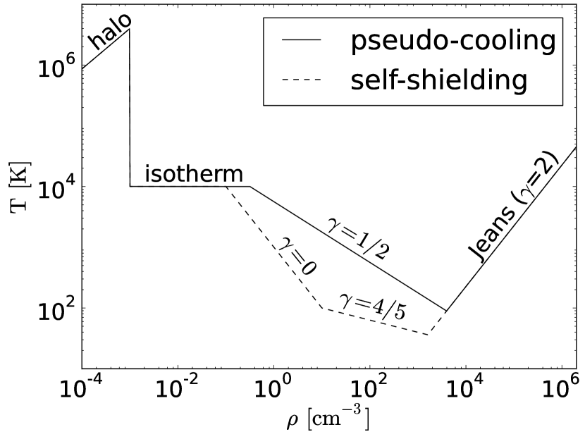
Figure 1.— Effective EoS for pseudo-cooling (solid line) and self-shielding (dashed line). Pseudo-cooling EoS mimics detailed balance between cooling and heating processes at 1/3 solar metallicity. Self-shielding EoS models the ability of the gas clouds to reach even lower temperatures by absorbing the interstellar radiation in their outer layers. The low density regime of index $\gamma=$ 5/3 corresponds to the hot virialized gas in the stellar halo. The Jeans polytrope of index $\gamma=$ 2 dominates high density regions, avoiding artificial fragmentation. For a given spatial resolution $d_{x,min}$ the Jeans polytrope becomes active at densities above $\approx$ 2761 cm^-3 $\times$ ($d_{x,min}$/1 pc)^-4/3 in the case of PC and $\approx$ 1023 cm^-3 $\times$ ($d_{x,min}$/1 pc)^-5/3 in the case of SS. The corresponding temperatures are $\approx$ 107 K $\times$ ($d_{x,min}$/1 pc)^2/3 and $\approx$ 40 K $\times$ ($d_{x,min}$/1 pc)^1/3 for PC and SS, respectively.

3. Galaxy sample

3.1. Initial conditions

We study models of a spiral galaxy resembling the Milky Way (hereafter MW), a disc galaxy similar to the Large Magellanic Cloud (LMC) and an irregular dwarf galaxy comparable to the Small Magellanic Cloud (SMC). We do not try to reproduce fine details for these galaxies, but propose models representing systems with different morphological and physical properties. Each simulation is performed in isolation and without cosmological evolution.

The details of the MW simulation can be found in Renaud et al. (2013). Here, this simulation is analyzed at resolution comparable to the resolution of other galaxy simulations in our sample, which is 1.5 pc, i.e. not at its maximal resolution. The parameters of all simulations are summarized in Table 1.

Simulations are labeled in a way to stress their principal difference which is related to EoS or metallicity parameter. Simulations in which the heating and cooling processes are evaluated have the value of metallicity in subscript. If the EoS is used instead, the subscript indicates the name of the equation of state. The most realistic cases are the LMC${}_{1.0{\mathrm{Z}}_{\odot}}$ and the SMC${}_{0.1{\mathrm{Z}}_{\odot}}$ simulations for LMC and SMC, respectively. The solar metallicity we have adopted in the LMC${}_{1.0{\mathrm{Z}}_{\odot}}$ simulation is higher than in the real LMC (1/2 Z_⊙; Russell & Dopita, 1992; Rolleston et al., 1996), but fairly representative of low-redshift and low mass disc galaxy that we intend to model. The metallicity of 1/10 Z_⊙ that we used in the SMC${}_{0.1{\mathrm{Z}}_{\odot}}$ simulation falls in the range of estimated values for the real SMC (1/5–1/20 Z_⊙; Russell & Dopita, 1992; Rolleston et al., 1999).

Table 1 Summary of model parameters.

	MWPC	LMC${}_{1.0{\mathrm{Z}}_{\odot}}$	LMCPC	LMCSS	SMC${}_{0.1{\mathrm{Z}}_{\odot}}$	SMC${}_{0.3{\mathrm{Z}}_{\odot}}$	SMC${}_{1.0{\mathrm{Z}}_{\odot}}$	SMCPC	SMCSS
EoS or metallicity [Z⊙]	PC	1.0	PC	SS	0.1	0.3	1.0	PC	SS
box length [kpc]	100	25			30
AMR coarse level	9	8			8
AMR fine level	21	14			15
maximal resolution [pc]	0.05	1.5			1.0
DM halo
mass [$\times$ $10^{9}$ M⊙]	453.0	8.0			1.2
number of particles [$\times$ $10^{5}$]	300.0	3.49			5.0
primordial stars
mass [$\times$ $10^{9}$ M⊙]	46.0	3.1			0.35
number of particles [$\times$ $10^{5}$]	300.0	5.75			2.15
gas
mass [$\times$ $10^{9}$ M⊙]	5.94	0.54			0.715
$\sim$ AMR cell number [$\times$ 106]	240	385	440	450	43	43	43	45	50
radial profile	exponential	exponential			exponential
scale radius [kpc]	6	3			1.3
radial truncation [kpc]	28	6			2.3
vertical profile	exponential	exponential			exponential
scale-height [kpc]	0.15	0.15			0.6
vertical truncation [kpc]	1.5	0.45			1.3
intergalactic density	$10^{-7}$	$10^{-7}$			$10^{-3}$
star formation
$\epsilon$	$3\%$	$3\%$			$3\%$
$\rho_{0}$ [cm-3]	$2\times 10^{3}$	$10^{2}$			$10^{2}$
stellar feedback
photo-ionization	✓	−			−
radiative pressure	✓	−			−
SNe	kinetic	thermic	kinetic	kinetic	thermic	thermic	thermic	kinetic	kinetic

3.2. Morphology

Figure 2 displays the surface gas density map of the three galaxies. MW_PC, a spiral galaxy, shows large variety of substructures: bar and spiral arms on the kpc-scale as well as dense clumps on the parsec scale (see Renaud et al., 2013, for details). LMC${}_{1.0{\mathrm{Z}}_{\odot}}$ is also a disc galaxy, but with a much less pronounced structure of spiral arms and more diffuse gas present in the inter-arm regions compared to MW_PC. SMC${}_{0.1{\mathrm{Z}}_{\odot}}$ is an irregular dwarf galaxy. Three major dense clumps can be seen within the irregular structure of the diffuse gas.

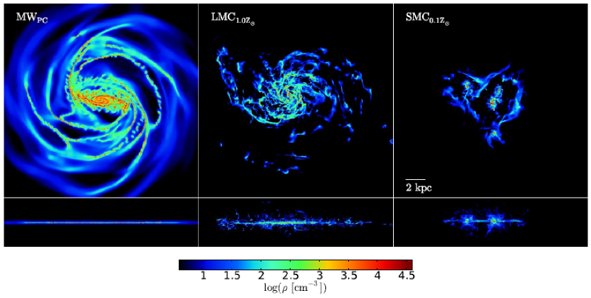
Figure 2.— Surface density of gas of the galaxies for our three simulations: MW_PC (left), LMC${}_{1.0{\mathrm{Z}}_{\odot}}$ (middle) and SMC${}_{0.1{\mathrm{Z}}_{\odot}}$ (right panel) seen face-on on the top and edge-on on the bottom panels. The box size of the face-on projection is 20$\times$20 kpc² and that of the edge-on projection is 20$\times$5 kpc².

3.3. Gas density PDF

The mass-weighted density probability distribution function (PDF) of the gas for MW_PC, LMC${}_{1.0{\mathrm{Z}}_{\odot}}$ and SMC${}_{0.1{\mathrm{Z}}_{\odot}}$ is shown in Figure 3. The MW_PC’s PDF has a log-normal shape, followed by a power-law tail at high densities ($\rho\gtrsim$ 1000 cm^-3) probed thanks to the high resolution reached in this simulation. Similarly, the LMC${}_{1.0{\mathrm{Z}}_{\odot}}$’s PDF can be approximated by a log-normal functional form in the density range from 10^-2 to 10² cm^-3 with and excess of dense gas with respect to a log-normal fit above density of about 100 cm^-3. Truncation possibly due to the resolution limit is visible at a density of $\sim$ 2$\times$10⁴ cm^-3. The PDF of the SMC${}_{0.1{\mathrm{Z}}_{\odot}}$ is rather irregular with two components, one at low densities ($\sim$ 10^-1 cm^-3) and the other one at high densities ($\sim$ 2$\times$ 10⁴ cm^-3). Such irregular PDF reveals the density contrast between diffuse gas and several high density clumps.

The shape of the density PDF is determined by global properties of galaxies and physical processes of their ISM. As suggested by Robertson & Kravtsov (2008), the density PDF can vary from galaxy to galaxy and that of a multiphase ISM can be constructed by summing several log-normal PDFs, each representing approximately an isothermal gas phase. Similarly, Dib & Burkert (2005) showed that the PDF of a bistable two-phase medium evolves into a bimodal form with a power-law tail at the high density-end in the presence of self-gravity (see also Elmegreen, 2011; Renaud et al., 2013). However, in most cases, a single, wider log-normal functional form is a reasonably good approximation of the PDF of disk galaxies up to $\gtrsim 10^{4}$ cm^-3 (see e.g. Tasker & Bryan, 2008; Agertz et al., 2009).

Note that SMC${}_{0.1{\mathrm{Z}}_{\odot}}$, which has a lower metallicity than LMC${}_{1.0{\mathrm{Z}}_{\odot}}$, is able to reach the highest densities. Metallicity is important for cooling: the more metallic gas is more efficient at cooling the gas down and should allow reaching higher densities. However, we do not observe such trend. This could indicate that factors other than thermal may be key in setting the gas distribution.

Another possible explanation could be a mismatch between the choices of threshold density $\rho_{0}$ for star formation and the metallicity in the LMC${}_{1.0{\mathrm{Z}}_{\odot}}$. If $\rho_{0}$ is chosen to be low, stars will form in an intermediate density medium, i.e. without the need of gravitational collapse of a cloud into a dense region. Furthermore, stellar feedback helps the destruction of the densest clumps which produces more intermediate-density gas and further prevents the gravitational contraction leading to high densities. The maximum density of the ISM is thus lower than with a high $\rho_{0}$ and the resulting PDF does not yield the classical high density power-law tail. However, in the case of LMC${}_{1.0{\mathrm{Z}}_{\odot}}$, the transition of the gas from high ($>$10³ – 10⁴ cm^-3) to intermediate densities (10 – 10² cm^-3, just below the actual $\rho_{0}$) due to the feedback would lead to a substantial reduction in the SFR (because of the $\rho_{\mathrm{SFR}}\propto\rho^{3/2}$ used in our model, the SFR is dominated by high-density gas). Consequently, feedback itself would be substantially reduced.

Another, more likely explanation is that SMC${}_{0.1{\mathrm{Z}}_{\odot}}$ contains a much higher gas fraction compared to LMC${}_{1.0{\mathrm{Z}}_{\odot}}$ (see Table 1) leading to a much lower value of Toomre parameter ($\mathrm{Q}\propto\Sigma_{\mathrm{gas}}^{-1}$) which allows SMC${}_{0.1{\mathrm{Z}}_{\odot}}$ to reach higher densities than in LMC${}_{1.0{\mathrm{Z}}_{\odot}}$.

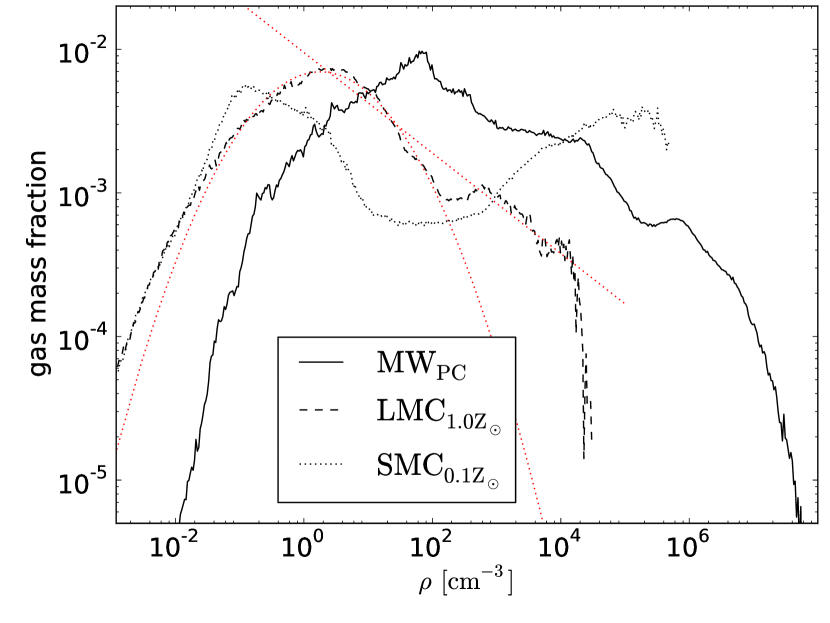
Figure 3.— Comparison of the mass-weighted density PDF in MW_PC at full resolution of 0.05 pc (solid line), LMC${}_{1.0{\mathrm{Z}}_{\odot}}$ (dashed line) and SMC${}_{0.1{\mathrm{Z}}_{\odot}}$ (dotted line). Approximated log-normal functional form and a power-law are shown for LMC${}_{1.0{\mathrm{Z}}_{\odot}}$ in red (see Renaud et al., 2013, Figure 10, for the best fit for MW_PC).

4. Analysis

To study the 100 pc scale properties of individual galaxies, analyzed regions are selected by examining the face-on projections of the gas distribution. We then consider sub-regions (referred to as beams throughout the paper) of 100$\times$100 pc² in the galactic plane and with galaxy scale-height along the line of sight. A study of the impact of the beam size is presented in Section 4.2.1.

4.1. Definitions

In a given beam, the effective Mach number $\mathcal{M}$ is defined as:

$$\mathcal{M}=\frac{\sigma_{v}}{\sqrt{3}}\frac{1}{{c_{s}}},$$ (1)

where $\sigma_{v}$ and ${c_{s}}$ are the mass-weighted velocity dispersion and the mass-weighted sound speed with respect to the beam, respectively, calculated as follows

$$\sigma_{v}=\sqrt{\frac{\sum\limits_{i}m_{i}v_{i}^{2}}{\sum\limits_{i}m_{i}}-\left(\frac{\sum\limits_{i}m_{i}v_{i}}{\sum\limits_{i}m_{i}}\right)^{2}},$$ (2)

and

$${c_{s}}=\sqrt{\frac{\sum\limits_{i}m_{i}T_{i}\gamma\frac{k_{\mathrm{B}}}{m_{\mathrm{H}}}}{\sum\limits_{i}m_{i}}}.$$ (3)

Summations are done over all AMR cells in the analyzed beam and the index $i$ refers to cell related quantities: $T_{i}$, $m_{i}$ and ${v}_{i}$ are the cell temperature, gas mass and speed, respectively. $\gamma=5/3$ is the adiabatic index for monoatomic gas, $m_{\mathrm{H}}$ is the mass of the hydrogen atom and $k_{\mathrm{B}}$ the Boltzmann constant.

An alternative to the above “beam-based” average could be to compute the mass-weighted $\mathcal{M}$ with a cell velocity dispersion itself calculated with respect to its closest cells, but we find that this does not lead to a significant difference in the results.

Temperature in the beam is computed as mass-weighted average:

$$T=\frac{\sum\limits_{i}m_{i}T_{i}}{\sum\limits_{i}m_{i}}.$$ (4)

To estimate the actual thickness of the star-forming regions within each beam, we apply Gaussian fit to 1D projection of the gas density along one of the mid-plane axes. The thickness is then defined as the full width at half maximum of the resulting fit. Although the estimation method of the thickness parameter is simplistic, the obtained values are in good agreement with visual inspection of density maps of individual star-forming regions.

Note that in our analysis we don’t use the SFR computed directly in the simulation. The main reason is that the conversion of gas into stars is modeled as a stochastic process leading to the discretization of the $\Sigma_{\mathrm{SFR}}$ values which make the analysis difficult by introducing more noise.

The SFR of a beam is estimated from the gas content of each cell by

$$\rho_{\star}=\epsilon\frac{\rho}{t_{\mathrm{ff}}}\propto\epsilon\rho^{3/2}\quad\text{for $\rho>\rho_{0}$},$$ (5)

where $\rho_{\star}$ is the local star formation rate density, $\rho$ is the density of gas in the cell, $\epsilon$ is the star formation efficiency per free-fall time $t_{\mathrm{ff}}=\sqrt{3\pi/(32G\rho)}$ and $\rho_{0}$ is the star formation threshold.

$\Sigma_{\mathrm{SFR}}$ is then given by

$$\Sigma_{\mathrm{SFR}}=\frac{\sum\limits_{i}{\rho_{\star}}_{i}V_{i}}{S},$$ (6)

where ${\rho_{\star}}_{i}$ and $V_{i}$ are the cell SFR density and volume, respectively and $S$ is the surface of the beam. Similarly, $\Sigma_{\mathrm{gas}}$ is

$$\Sigma_{gas}=\frac{\sum\limits_{i}\rho_{i}V_{i}}{S},$$ (7)

with $\rho_{i}$ representing the cell gas density.

4.2. Tests

4.2.1 Beam size effects

Our choice of the beam size is related to the adopted analytical formalism which is tightly linked to the turbulence-driven structure of the ISM. Supersonically turbulent isothermal gas is found to be well described by a log-normal probability distribution function. However, once these hypotheses about the state of gas are relaxed, strictly log-normal PDF is not recovered. The PDFs of the density field in our sample of galaxies are close to, but not exactly log-normal functional forms when all scales are considered (see Section 3.3). Individual beams should be large enough to be representative samples of star-forming regions at different evolutionary stages. In addition, the choice of the beam size is somehow linked to the turbulence and its cascade from large scales where the turbulence is injected, down to the small scales, where the energy dissipation overcomes its transfer. In order to capture the turbulent cascade, the size of the beam should not be too large compared to the injection scale, nor too small compared to the dissipation scale. In the former case, the simulation would capture other processes than turbulence and in the latter case, turbulence would be already dissipated.

To estimate the impact of the size of the beam, we compare the results in the $\Sigma_{\mathrm{gas}}$–$\Sigma_{\mathrm{SFR}}$ plane obtained by varying the beam width by a factor of 2.5 with respect to the one used in analysis. Figure 4 shows the comparison for the MW_PC simulation. Increased beam size leads to an overall reduction of $\Sigma_{\mathrm{gas}}$ for the beam, which can be understood as a consequence of decreased volume fraction occupied by the dense gas. On the contrary, smaller beam size allows reaching higher values of $\Sigma_{\mathrm{SFR}}$. This comparison suggests that the position of points in the $\Sigma_{\mathrm{gas}}$–$\Sigma_{\mathrm{SFR}}$ plane depends on the considered spatial scale. Schruba et al. (2010) found such dependence in the study of the Local Group spiral galaxy M33. Similarly, Lada et al. (2013) found a more efficient SF at scales of molecular clouds, indicating that caution should be used when comparing SF relations involving different spatial scales.

However, the global behavior of the $\Sigma_{\mathrm{gas}}$–$\Sigma_{\mathrm{SFR}}$ does not seem to be strongly affected by the size of the beam, at least for the range of sizes that we explored.

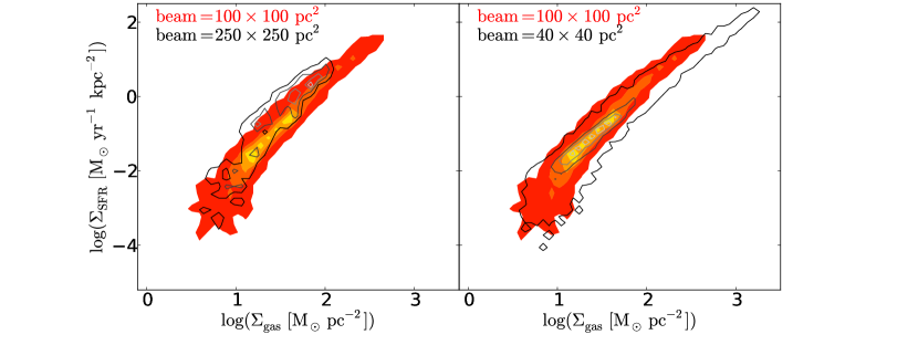
Figure 4.— The effect of beam size on the $\Sigma_{\mathrm{gas}}$–$\Sigma_{\mathrm{SFR}}$ relation in the MW_PC simulation. The two panels show the effect of varying the beam width by a factor of 2.5 (black contours) with respect to the one used in analysis (colored filled contours). When increasing the beam size, the dense gas represents smaller and smaller volume fraction which leads to an overall reduction of $\Sigma_{\mathrm{gas}}$ for the beam. The color coding of the two-dimensional normalized histogram corresponds to the 0.3, 0.5, 0.8 and 1.0 contour levels.

4.2.2 Parsec and sub-parsec physics

We remind that the MW_PC simulation is analyzed at the resolution of 1.5 pc which is different from its maximal resolution of 0.05 pc. To study the impact of the resolution, we compare in Figure 5 the $\Sigma_{\mathrm{gas}}$–$\Sigma_{\mathrm{SFR}}$ relation for these two resolutions. Sub-parsec physics does not influence our results at low and intermediate surface gas densities, but it plays a role in densest regions, where it leads to higher values of $\Sigma_{\mathrm{SFR}}$. The increased resolution leads to the modification of structures mainly at high densities which translates into higher values of $\Sigma_{\mathrm{SFR}}$ computed at fixed 100 pc scale.

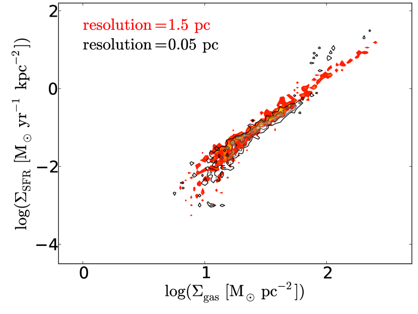
Figure 5.— The impact of resolution on the $\Sigma_{\mathrm{gas}}$–$\Sigma_{\mathrm{SFR}}$ relation in the MW_PC simulation. The maximal resolution of 0.05 pc (black contours) is compared to the resolution of 1.5 pc (colored filled contours), at which the entire analysis is performed. No significant difference is noticeable at low and intermediate surface densities of gas. At high $\Sigma_{\mathrm{gas}}$, $\Sigma_{\mathrm{SFR}}$ tends to be higher at the resolution of 0.05 pc. The color coding of contour levels is as in Figure 4.

5. Results

In order to have a significant amount of data, we use several snapshots in the analysis of the LMC and SMC galaxies.

5.1. Global parameters

Figure 6 shows the impact of metallicity on the $\Sigma_{\mathrm{SFR}}$. The left panel compares two systems with comparable metallicities, 0.1 Z_⊙ and 0.3 Z_⊙, while on the right panel, two more extreme metallicities are compared, 0.1 Z_⊙ and 1.0 Z_⊙. In the region below the break, high metallicity systems tend to have higher $\Sigma_{\mathrm{SFR}}$ for a fixed value of $\Sigma_{\mathrm{gas}}$ than systems with lower metallicity.

The impact of the EoS on the SFR is presented in Figure 7. The SMC${}_{0.1{\mathrm{Z}}_{\odot}}$ simulation is compared to that of SMC_PC, using the EoS of pseudo-cooling and to that of SMC_SS with the EoS of self-shielding. The similarity of two contour plots on the left panel shows that the pseudo-cooling EoS is a good approximation to the actual heating and cooling processes even for a slightly lower metallicity in this case (we remind that the pseudo-cooling EoS is derived using the metallicity of 1/3 Z_⊙; see Section 2.2). In the case of the self-shielding EoS, for a given value of $\Sigma_{\mathrm{gas}}$, $\Sigma_{\mathrm{SFR}}$ tends to be higher compared to that of the simulation with metallicity of 0.1 Z_⊙.

We do not assume any metallicity gradient in the gas, nor chemical evolution. We use the model for self-shielding without an implicit metallicity dependence, similarly to the work of Dobbs et al. (2008). As shown in Figure 7, the self-shielding EoS leads to higher $\Sigma_{\mathrm{SFR}}$ for fixed $\Sigma_{\mathrm{gas}}$ compared to the model of SMC with metallicity of 0.1 Z_⊙.

The existence of the break in the Schmidt-Kennicutt relation in our models does not seem to depend on self-shielding effects. The exact position of this break is however sensitive to metallicity: the slope at low $\Sigma_{\mathrm{gas}}$, i.e. below the break, is higher in metal-poor galaxies as shown on Figure 6. Similar metallicity dependent position of the break is present in the theoretical model of Krumholz et al. (2009) including the effect of hydrogen self-shielding which in turn determines the amount of gas in molecular form. In addition, Dib (2011) explored the metallicity-dependent feedback and found that it can lead to a modification of the position of the break for a given metallicity-dependent molecular gas fraction. It is clear that self-shielding has an impact on the Schmidt-Kennicutt relation (see right panel of the Figure 7), but it does not seem to be the only factor determining the presence of the break.

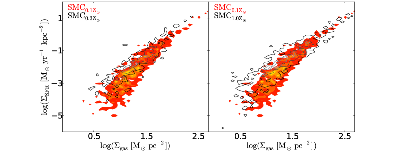
Figure 6.— The impact of gas metallicity on the $\Sigma_{\mathrm{gas}}$–$\Sigma_{\mathrm{SFR}}$ relation in the model of SMC. The left panel shows two simulations of the SMC with comparable metallicities: 0.1 Z_⊙(colored filled contours) and 0.3 Z_⊙ (black contours). The right panel compares the effect of gas metallicity of 0.1 Z_⊙ with that of 1.0 Z_⊙. Gas cooling rates increase with metallicity, which translates into increased $\Sigma_{\mathrm{SFR}}$ for a fixed value of $\Sigma_{\mathrm{gas}}$ in the region of the break. The color coding of contour levels is as in Figure 4.

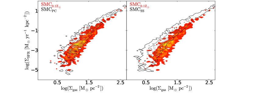
Figure 7.— Comparison of the $\Sigma_{\mathrm{gas}}$–$\Sigma_{\mathrm{SFR}}$ relation in SMC${}_{0.1{\mathrm{Z}}_{\odot}}$ (colored filled contours) to that of SMC_PC (black contours) in the left panel and to that of SMC_SS (black contours) in the right panel). The color coding of contour levels is as in Figure 4.

5.2. Local parameters

5.2.1 Mach number

In Figure 8 we show how the $\Sigma_{\mathrm{gas}}$ – $\Sigma_{\mathrm{SFR}}$ relation depends on the Mach number, temperature and velocity dispersion calculated using the Equations 1, 4 and 2, respectively. We show the example of MW_PC, but we obtain qualitatively similar results for all other galaxies. The Mach number dependence for MW_PC, SMC${}_{0.1{\mathrm{Z}}_{\odot}}$ and LMC${}_{1.0{\mathrm{Z}}_{\odot}}$ is displayed in Figure 9.

Two regimes in the star formation relation are identified. The points located in the region below the break have typically Mach numbers with values below unity. Furthermore, for a given $\Sigma_{\mathrm{gas}}$, $\Sigma_{\mathrm{SFR}}$ increases with increasing Mach number. At high surface densities of gas, $\Sigma_{\mathrm{SFR}}$ and $\Sigma_{\mathrm{gas}}$ are found to be correlated. The gas reservoirs that happen to be in this regime of efficient star formation tend to have supersonic velocity dispersions.

Both the temperature and velocity dispersion contribute to the resulting Mach number dependence in the star formation relation. Despite the variation in temperature, the overall variation in Mach number relies on $\sigma_{v}$. The velocity dispersion of the ISM can be increased by several processes. Among them Bournaud et al. (2010) found, in simulations similar to those analyzed here, self-gravity to play the dominant role, compared to stellar feedback. Therefore, by increasing the velocity dispersion, self-gravity sets the level of turbulence, i.e. the compression of gas and thus the SF. This suggests that the power-law part of the $\Sigma_{\mathrm{gas}}$–$\Sigma_{\mathrm{SFR}}$ relation arises from self-gravity at high Mach number, while this connection is weaker in the break.

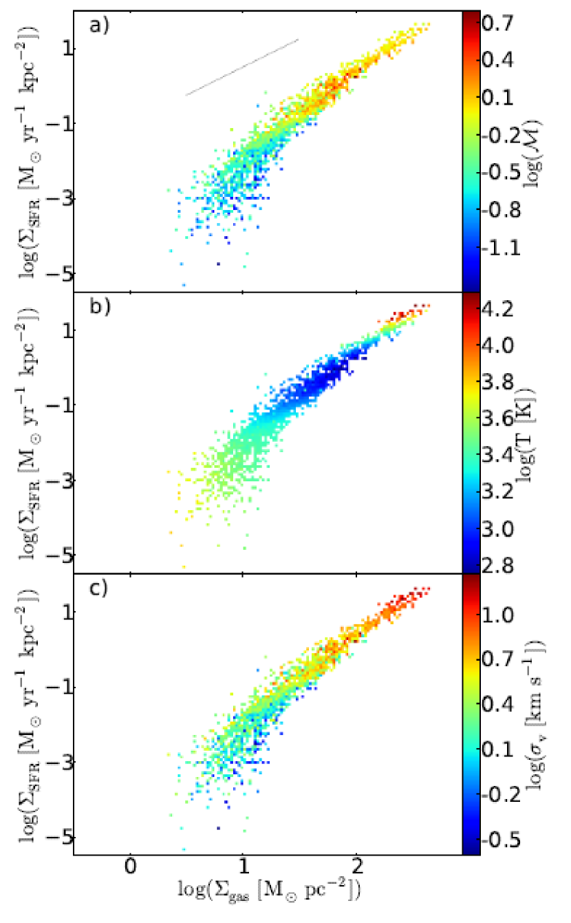
Figure 8.— The local surface density of the star formation rate as a function of surface density of gas for the MW_PC model. The color indicates the Mach number (panel a), temperature (panel b) and velocity dispersion (panel c) in each beam. The dotted line indicates a power-law of index $3/2$. Note that regions at high $\Sigma_{\mathrm{gas}}$ and high $\Sigma_{\mathrm{SFR}}$ that have high temperatures represent unresolved dense gas situated on the Jeans polytrope (see Section 2.2).

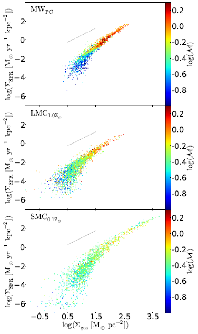
Figure 9.— The local surface density of the star formation rate as a function of surface density of gas for MW_PC (top panel), LMC${}_{1.0{\mathrm{Z}}_{\odot}}$ (middle) and SMC${}_{0.1{\mathrm{Z}}_{\odot}}$ (bottom). The color indicates the Mach number. The dotted line indicates a power-law of index $3/2$.

5.2.2 Vertical scale of the gas

Figure 10 shows the variation of the $\Sigma_{\mathrm{gas}}$–$\Sigma_{\mathrm{SFR}}$ relation with the thickness of the star-forming regions in SMC${}_{0.1{\mathrm{Z}}_{\odot}}$. For a given surface gas density, thicker regions tend to have lower surface star formation density. This relation between $\Sigma_{\mathrm{SFR}}$ and the thickness parameter at fixed $\Sigma_{\mathrm{gas}}$ results from the Equation 5 relating the volume density of gas with that of star formation rate.

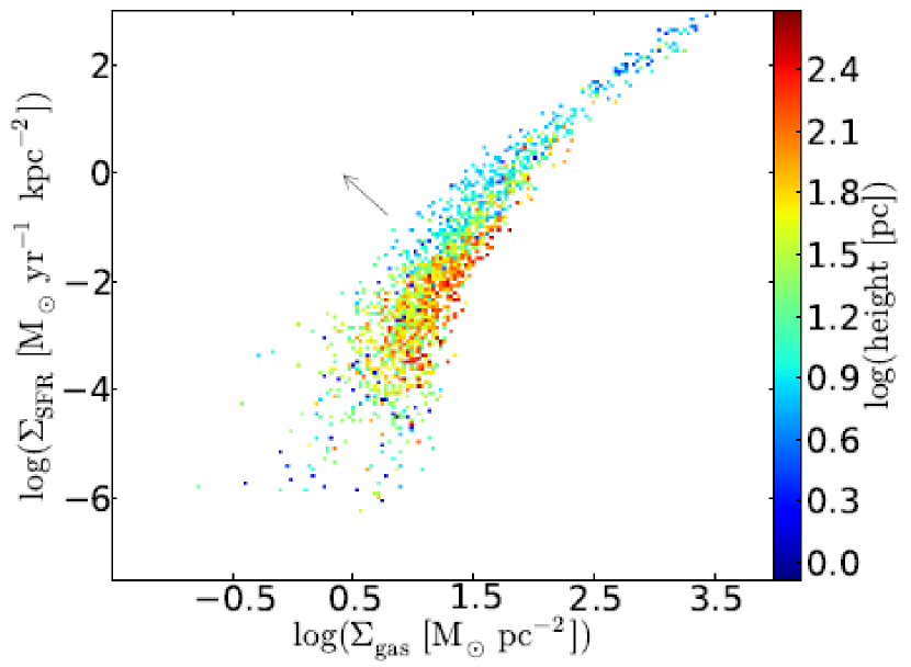
Figure 10.— The local surface density of the star formation rate as a function of surface density of gas for the SMC${}_{0.1{\mathrm{Z}}_{\odot}}$ model. The color represents the thickness of star-forming region. The arrow indicates the direction in the measured scale-height of the gas from higher to lower values.

6. Discussion

6.1. Comparison with observations

Most spatially resolved studies of spiral galaxies find the presence of a power-law $\Sigma_{\mathrm{gas}}$–$\Sigma_{\mathrm{SFR}}$ relation with a break at surface gas densities of the order of a few M${}_{\odot}\,\mathrm{pc}^{-2}$ (see Kennicutt & Evans, 2012, and references therein). The slope of the power-law relation in the high surface-density regime is found to be in the range 1.2–1.6 when total (molecular plus atomic) gas surface density is considered.

Less agreement about the power-law slope in observations is reached when molecular-gas surface density is considered solely. Some recent studies (e.g. Eales et al., 2010; Rahman et al., 2011; Leroy et al., 2013) have reported an approximately linear relation between the surface density of star formation rate and the surface density of molecular gas. Other studies (e.g. Kennicutt et al., 2007; Verley et al., 2010; Liu et al., 2011) have found a much steeper relation, with a slope in the range 1.2–1.7, similar to that of integrated measurements (Kennicutt, 1998). This discrepancy between different results in observations is still debated. A possible interpretation of the sublinear relation was recently proposed by Shetty et al. (2013). They suggest that the CO emission used in the estimation of $\Sigma_{\mathrm{gas}}$ is not all necessarily associated with SF. Not subtracting off such a diffuse component could lead to a slope close to unity.

The distribution of data points from the observations of the SMC (Bolatto et al., 2011) in the $\Sigma_{\mathrm{gas}}$–$\Sigma_{\mathrm{SFR}}$ plane has a similar shape than that of spiral galaxies, but is noticeably shifted toward higher total $\Sigma_{\mathrm{gas}}$.

In Figure 11, we show three of our models: MW_PC, SMC${}_{0.1{\mathrm{Z}}_{\odot}}$ and LMC${}_{1.0{\mathrm{Z}}_{\odot}}$ in the $\Sigma_{\mathrm{gas}}$–$\Sigma_{\mathrm{SFR}}$ plane. The MW_PC and the LMC${}_{1.0{\mathrm{Z}}_{\odot}}$ models lie in the loci of observed spiral galaxies (e.g. Kennicutt, 1998; Kennicutt et al., 2007; Bigiel et al., 2008). Our SMC${}_{0.1{\mathrm{Z}}_{\odot}}$ model has a lower $\Sigma_{\mathrm{SFR}}$ for a given $\Sigma_{\mathrm{gas}}$ when compared to both the MW_PC and the LMC${}_{1.0{\mathrm{Z}}_{\odot}}$ models. The region below the break of our SMC${}_{0.1{\mathrm{Z}}_{\odot}}$ model is located at slightly lower $\Sigma_{\mathrm{gas}}$ than the real Small Magellanic Cloud, but its displacement with respect to spiral galaxies (MW and LMC) is well reproduced (Figure 11). In our simulations, Equation 5 sets the slope of power-law relation with the value of 1.5. A shallower relation, closer to the observed values, might be reached by accounting for a stronger regulation of star formation (e.g. pre-SN stellar feedback, see Renaud et al. 2012), but this slope change has not been demonstrated by simulations yet.

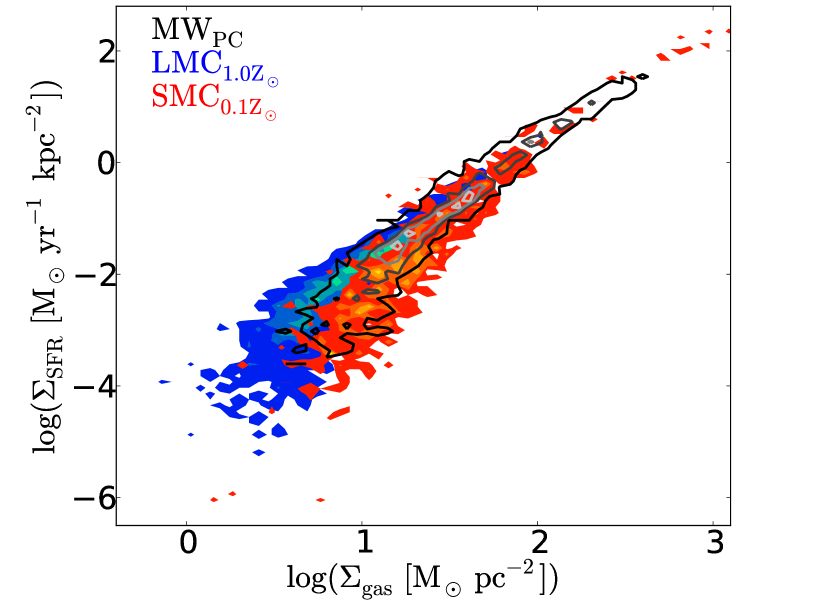
Figure 11.— Comparison of MW_PC, LMC${}_{1.0{\mathrm{Z}}_{\odot}}$ and SMC${}_{0.1{\mathrm{Z}}_{\odot}}$. The color coding of contour levels is as in Figure 4.

6.2. Interpretation of threshold

The existence of the break in the $\Sigma_{\mathrm{gas}}$–$\Sigma_{\mathrm{SFR}}$ relation is, in our models, equivalent of having a non-zero value of the volume density threshold in the local, three dimensional star formation relation. Setting no threshold leads to a power-law relation without a break.

Figure 12 shows that the value of the density threshold $\rho_{0}$ that we have used in our analysis has an impact on the $\Sigma_{\mathrm{gas}}$–$\Sigma_{\mathrm{SFR}}$ relation. Changing the value of $\rho_{0}$ changes the slope at low $\Sigma_{\mathrm{gas}}$ in the $\Sigma_{\mathrm{gas}}$–$\Sigma_{\mathrm{SFR}}$ relation (Figure 12). This could suggest that the transition from the inefficient to the power-law regime could be due to the density threshold $\rho_{0}$ we imposed by hand in the star formation law (see Equation 5). However, we have checked that the deviation from the power-law regime occurs at $\mathcal{M}\approx$ 1, independently of $\rho_{0}$. In addition, in Figure 9, we have shown that beams located in the break tend to have $\mathcal{M}$ below unity, while regions at high $\Sigma_{\mathrm{gas}}$ are mostly supersonic.

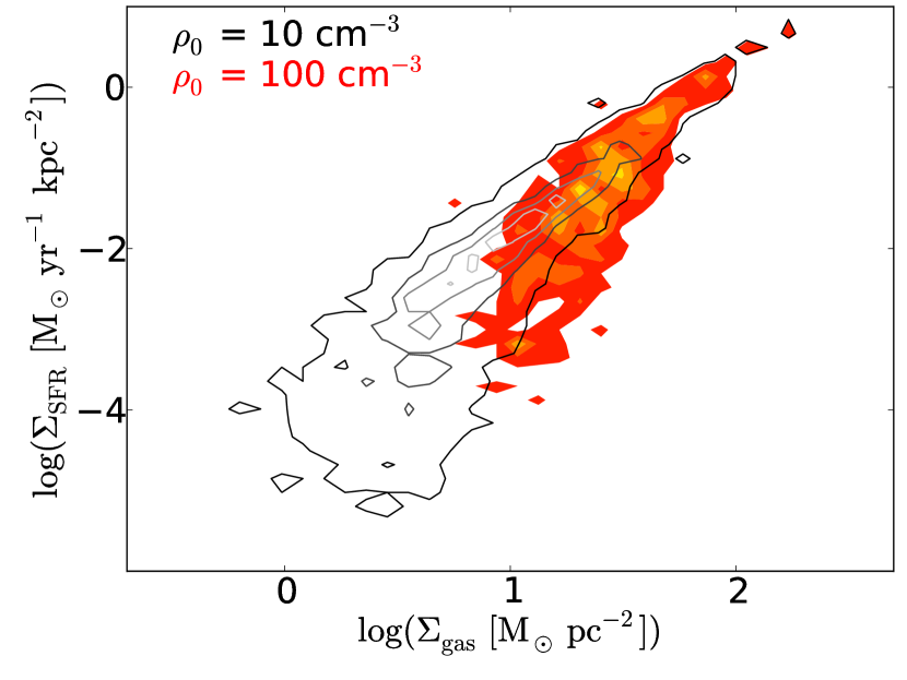
Figure 12.— Comparison of the $\Sigma_{\mathrm{gas}}$–$\Sigma_{\mathrm{SFR}}$ relation in the LMC${}_{1.0{\mathrm{Z}}_{\odot}}$ simulation with the star formation volume density threshold $\rho_{0}$=10 cm^-3 (black contours) to that with $\rho_{0}$=100 cm^-3 (colored filled contours). The color coding of contour levels is as in Figure 4.

To better understand the behavior of the ISM in our simulations, we show in Figure 13 the Mach number as a function of average volume density of gas $\left<\rho\right>$ in the beam for MW_PC. The Mach number varies with the average density as $\mathcal{M}\propto\left<\rho\right>^{0.5}$, similarly to the two-phase turbulent flow studied by Audit & Hennebelle (2010). Although caution should be used when doing such comparison (temperature and velocity dispersion vary with density differently in both models), the onset of the supersonic regime, i.e. the transition from an inefficient regime to a power-law, happens at densities of $\approx 10$ cm^-3(see also Audit & Hennebelle, 2010, their Figures 4 and 9).

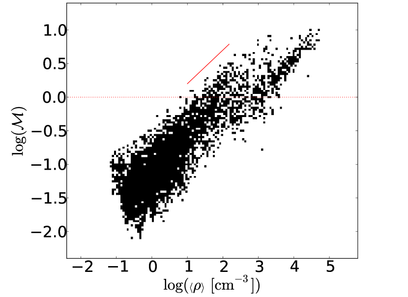
Figure 13.— The Mach number as a function of the average volume density of gas computed in beams of 100$\times$100$\times$100 pc³, for MW_PC. The solid line corresponds to $\mathcal{M}\propto\left<\rho\right>^{0.5}$ (Audit & Hennebelle, 2010, Figure 9).

Other interpretations of the observed break are possible. The $\Sigma_{\mathrm{gas}}$–$\Sigma_{\mathrm{SFR}}$ relation could be an effect of the galactic radial distance with low $\Sigma_{\mathrm{gas}}$ at large radius and high $\Sigma_{\mathrm{gas}}$ at small radius, as found by Kennicutt et al. (2007) and Bigiel et al. (2008). The break could then be explained as a consequence of the drop in the average volume density in the outer regions of galaxies as proposed by Barnes et al. (2012). However, Figure 14 shows no such radial dependence for $\Sigma_{\mathrm{gas}}$ nor $\Sigma_{\mathrm{SFR}}$. Star-forming regions in outer parts of a galaxy can exhibit both star formation regimes. A possible explanation why we do not see any radial dependence in our simulations may be a missing metallicity gradient. The outer regions of our simulated galaxies have the same metallicity than the innermost regions, thus the metallicity is probably too high at the edge of disk and allows for an efficient cooling and consequently an efficient star formation while it may lie in the break regime otherwise.

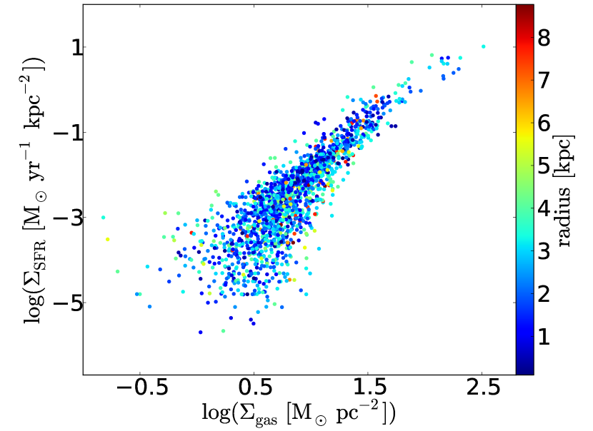
Figure 14.— The local surface density of the star formation rate as a function of surface density of gas for LMC${}_{1.0{\mathrm{Z}}_{\odot}}$. Color indicates the radial distance of the beam in kpc.

When azimuthally averaged, $\Sigma_{\mathrm{gas}}$ and $\Sigma_{\mathrm{SFR}}$ both decline steadily as a function of radius in many galaxies despite different morphologies (see Bigiel et al. 2008 for a sample of nearby spiral galaxies and Leroy et al. 2009 for CO intensity radial profiles for the same sample). Figure 15 shows $\Sigma_{\mathrm{gas}}$ and $\Sigma_{\mathrm{SFR}}$ as functions of radius for LMC${}_{1.0{\mathrm{Z}}_{\odot}}$. Both radial profiles decline with galactic radius as in observed spiral galaxies.

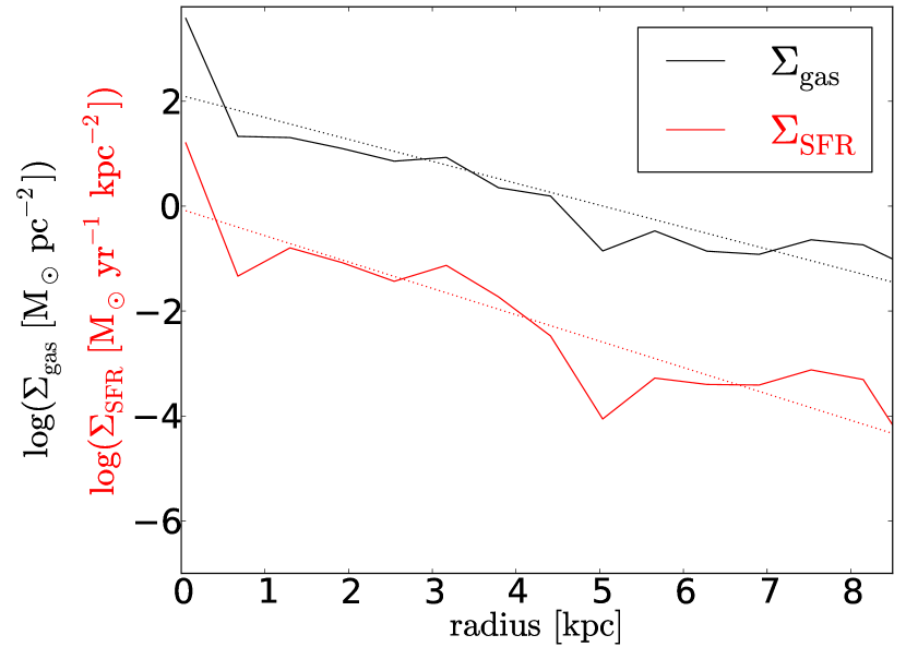
Figure 15.— Radial profiles of azimuthally averaged $\Sigma_{\mathrm{gas}}$ (black) and $\Sigma_{\mathrm{SFR}}$ (red) for LMC${}_{1.0{\mathrm{Z}}_{\odot}}$. Dotted lines correspond to exponential fits.

Another alternative explanation for the existence of the break is that it corresponds to the transition from atomic to molecular hydrogen (Krumholz et al., 2009). According to this scenario, the transition from atomic to molecular hydrogen and the subsequent star formation depend on local conditions that vary with galactic radius, e.g. metallicity, gas pressure and shear. Bigiel et al. (2008) found such radial dependence in the sample of nearby galaxies in agreement with the findings of Wong & Blitz (2002) and the threshold interpretations of e.g. Kennicutt (1989), Martin & Kennicutt (2001) and Leroy et al. (2008). Similar results are reproduced in some simulations, e.g. Halle & Combes (2013), who find that molecular gas is a better tracer of star formation than atomic gas and plays an important role in the low surface density regions of galaxies by allowing for more efficient star formation. However, our models that do not include chemodynamics, are able to reproduce the observed break at low $\Sigma_{\mathrm{gas}}$. Therefore, this seems to indicate that the presence of molecules is not a necessary condition to trigger the process of star formation. However, we acknowledge numerous observational evidences showing that molecules are involved at a later stage of the SF process.

To summarize, we consider two representative beams having the same $\Sigma_{\mathrm{gas}}$, but different $\Sigma_{\mathrm{SFR}}$ (Figure 16). These beams have similar average volume densities $\left<\rho\right>$ which can be several orders of magnitude smaller than $\rho_{0}$. However, the beam that happens to have the highest $\Sigma_{\mathrm{SFR}}$ has always the highest Mach number, as previously suggested by Figure 9. We have argued above that the density threshold $\rho_{0}$, the thickness of the star-forming regions and the molecules do not have impact on the transition from the regime of inefficient star formation to the efficient power-law regime. The role of the artificial threshold $\rho_{0}$ imposed in the simulations is to set a frontier between the diffuse non-star-forming gas and the star-forming component, but not to tune the efficiency of star formation per se. Therefore at a given $\Sigma_{\mathrm{gas}}$, this efficiency depends mostly on the level of turbulence ($\mathcal{M}$), i.e. the compression of the ISM.

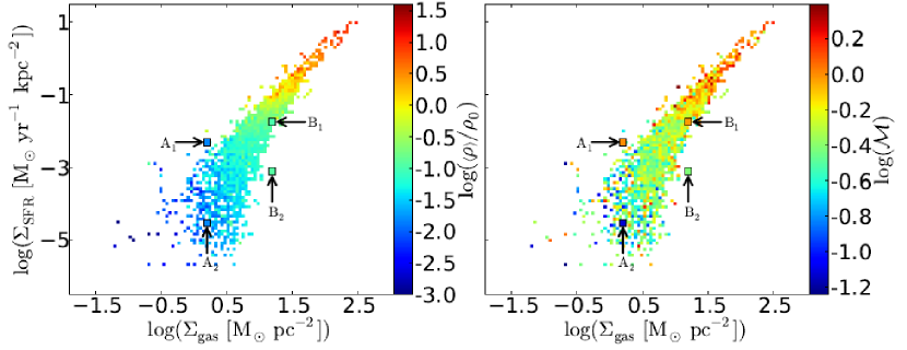
Figure 16.— The volume density normalized to the threshold density $\rho_{0}$=10 cm^-3 (left panel) and the Mach number (right panel) for the LMC${}_{1.0{\mathrm{Z}}_{\odot}}$ simulation, as in Figure 9. Two pairs of beams (A₁–A₂ and B₁–B₂) are highlighted in each panel. Within each pair, the two beams are chosen to have the same value of $\Sigma_{\mathrm{gas}}$ and a similar value of $\left<\rho\right>/\rho_{0}$. Beams with higher $\Sigma_{\mathrm{SFR}}$ at fixed $\Sigma_{\mathrm{gas}}$ have a higher Mach number. The two pairs of beams have larger size for clarity reasons.

Renaud et al. (2012) proposed that the break indeed corresponds to the onset of supersonic turbulence which, by generating shocks, triggers gravitational instabilities leading to star formation. In Figures 17 and 18, we compare simulations of MW_PC and SMC${}_{0.1{\mathrm{Z}}_{\odot}}$ with the analytical model of Renaud et al. (2012). In this model, the relation between $\Sigma_{\mathrm{gas}}$ and $\Sigma_{\mathrm{SFR}}$ depends on three parameters: the Mach number $\mathcal{M}$, the scale-height $h$ and the star formation volume density threshold $\rho_{0}$. We do not compare each star-forming region in the simulation with the model, but we are rather interested in what values these parameters should take to obtain upper and lower limits for simulated data. The break is in the subsonic regime (measured values of $\mathcal{M}$ are below unity) which corresponds to the regime where the analytical model deviates from its asymptotic behavior (at high $\Sigma_{\mathrm{gas}}$). In this regime the scale-heights of the beams set the efficiency of star formation spanning the range given by the model and quantitatively in accordance with the values measured in the simulations (Figure 10). In the analytical model, the power-law regime can be reached even with the Mach number below unity (red curve). However, our simulations do not probe this area of the $\Sigma_{\mathrm{gas}}$–$\Sigma_{\mathrm{SFR}}$ plane: the data points in the power-law regime are exclusively supersonic and can only be described by a model with the Mach number above unity (black curve).

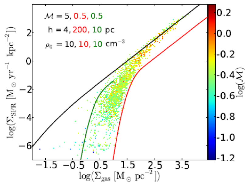
Figure 17.— SMC${}_{0.1{\mathrm{Z}}_{\odot}}$: comparison with the Renaud et al. (2012) model with three sets of parameters (indicated in the legend). The black curve matches the supersonic regime of efficient star formation, while the green and the red curves represent upper and lower limits for the regime of the break, where the star formation is inefficient. The $h$ parameter is in agreement with values measured in the simulation (see Figure 10).

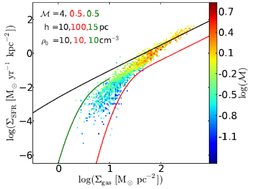
Figure 18.— MW_PC: comparison with the Renaud et al. (2012) model. As in Figure 17, the supersonic regime is compared to the model prediction and similarly, the subsonic regime at low $\Sigma_{\mathrm{gas}}$ is situated between the curves characterized by the Mach number lower than unity for the measured thickness.

6.3. Metallicity

In Figure 6, we have shown that the exact position of the break in the $\Sigma_{\mathrm{gas}}$–$\Sigma_{\mathrm{SFR}}$ plane depends on metallicity. A comparison of different metallicities in otherwise identical systems shows that the slope at low $\Sigma_{\mathrm{gas}}$ has a greater value in metal-poor galaxies. Figure 3 suggests that metallicity is not the only factor determining the gas density distribution in our simulations. Similar lack of direct dependence of the fraction of dense gas on metallicity is found when simulations of the SMC with different metallicities are compared (not shown here). Thus the slope at low $\Sigma_{\mathrm{gas}}$ cannot be explained by the presence of a higher fraction of dense gas in systems with higher metallicity compared to systems with lower metallicity. However, metallicity has an impact on star formation, even though indirect. Metallicity directly influences the temperature of the gas: higher the metallicity, more efficient the cooling therefore the temperature and, in turn, impacts the Mach number. In Figure 19, we show Mach numbers for SMC${}_{1.0{\mathrm{Z}}_{\odot}}$ and SMC${}_{0.1{\mathrm{Z}}_{\odot}}$. Higher values of Mach number are reached in galaxy with higher metallicity.

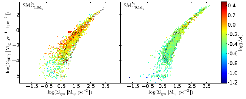
Figure 19.— As in Figure 6, the effect of gas metallicity on the $\Sigma_{\mathrm{gas}}$–$\Sigma_{\mathrm{SFR}}$ relation in the model of SMC is represented. Colors indicate the Mach number in the simulation of the SMC with metallicity of 1.0 Z_⊙ on the left panel and the simulation of the SMC with metallicity of 0.1 Z_⊙ on the right panel. In both panels the black contours are those of the simulation of the SMC${}_{0.1{\mathrm{Z}}_{\odot}}$, shown for reference.

This work does not include metallicity-dependent self-shielding and feedback. Accounting for them, Dib (2011) showed that both the fraction of gas in molecular form and the efficiency of star formation per unit time depend on metallicity. This leads to the metallicity dependent $\Sigma_{\mathrm{gas}}$–$\Sigma_{\mathrm{SFR}}$ relation at any $\Sigma_{\mathrm{gas}}$.

7. Summary

In this paper, we study the star formation relations and thresholds at 100 pc scale in a sample of low-redshift simulated galaxies. These include simulations representative of Milky Way-like spiral galaxy, the Large and the Small Magellanic Clouds. We analyze the role of interstellar turbulence, gas cooling, and geometry in drawing these relations, by investigating the dependence of the star formation on three parameters: the Mach number, the thickness of the star-forming region and the star formation volume density threshold. We compare the simulated data with the idealized model for star formation of Renaud et al. (2012).

Our main findings are as follows:

1. Our simulations support an interpretation of the surface density threshold for efficient star formation as the typical density for the onset of supersonic turbulence in dense gas, as proposed theoretically by Renaud et al. (2012). For all analyzed systems, we obtain qualitatively the same result: regions located below the break are dominated by subsonic turbulence, while turbulence tends to be supersonic in those located in the power-law regime, .

2. The distribution of the ISM of a galaxy in the $\Sigma_{\mathrm{gas}}$–$\Sigma_{\mathrm{SFR}}$ plane (mainly the position of the break) is sensitive to metallicity, but always correlated with the Mach number as detailed above. When different metallicities are considered for otherwise identical systems, $\Sigma_{\mathrm{SFR}}$ increases with the metallicity. When different systems with same metallicities are considered (compare Figure 11 for LMC${}_{1.0{\mathrm{Z}}_{\odot}}$ and Figure 6 for SMC${}_{1.0{\mathrm{Z}}_{\odot}}$), roughly the same position in the $\Sigma_{\mathrm{gas}}$–$\Sigma_{\mathrm{SFR}}$ plot is obtained. This can explain observations of low-efficiency star formation in relatively dense gas in SMC-like dwarf galaxies. The driving physical parameter is still the onset of supersonic turbulence, but this onset is harder to reach at moderate gas densities in lower-metallicity systems that can preserve warmer gas.

3. The vertical spread in the $\Sigma_{\mathrm{gas}}$–$\Sigma_{\mathrm{SFR}}$ plot is given by the interplay between different parameters of star-forming regions. Figures 17 and 18 show a reasonable agreement between simulations and the analytic model of Renaud et al. (2012), confirming that this idealized model provides a viable description of star formation in a turbulent ISM compared to more realistic simulations of self-gravitating systems with star formation and feedback. The values of the model parameters (Mach number, thickness and density threshold) characterizing the points in $\Sigma_{\mathrm{gas}}$–$\Sigma_{\mathrm{SFR}}$ plane are close to the values measured in simulations.

Several other models (e.g. Krumholz et al., 2009) have proposed that self-shielding alone is efficient at producing giant molecular clouds and triggering SF. Indeed, this effect cools the gas down at high density, thus enhancing the fragmentation of the ISM, but also lowering the sound speed, i.e. increasing the level of turbulence. Both the compression of the ISM by supersonic turbulence and the fragmenting effect from self-shielding increase with metallicity. Having neglected the dependence of self-shielding on metallicity, our results emphasize only the role of supersonic turbulence in our most metal rich examples. Combining the two effects would lead to a higher efficiency of star formation than either effect alone.

At the scale of clouds, the gravitational collapse is known to trigger SF. However, at larger scales, in galactic structures like spiral arms, we found that the injection of turbulence by self-gravity (and possibly by other processes like shear and feedback) can drive the compression of the gas, leading to SF. In this view, an external trigger like supersonic turbulence could be a sufficient condition to from stars, without necessarily invoking the collapse of large galactic regions ($\sim$ 100 pc) prior to turbulent compression – only compressed regions need to eventually collapse into stars.

References

- Agertz et al. (2009) Agertz, O., Lake, G., Teyssier, R., et al. 2009, MNRAS, 392, 294
- Agertz et al. (2011) Agertz, O., Teyssier, R., & Moore, B. 2011, MNRAS, 410, 1391
- Audit & Hennebelle (2010) Audit, E., & Hennebelle, P. 2010, A&A, 511, A76
- Barnes et al. (2012) Barnes, K. L., van Zee, L., Côté, S., & Schade, D. 2012, ApJ, 757, 64
- Bigiel et al. (2008) Bigiel, F., Leroy, A., Walter, F., et al. 2008, AJ, 136, 2846
- Boissier et al. (2003) Boissier, S., Prantzos, N., Boselli, A., & Gavazzi, G. 2003, MNRAS, 346, 1215
- Bolatto et al. (2011) Bolatto, A. D., Leroy, A. K., Jameson, K., et al. 2011, ApJ, 741, 12
- Bonnell et al. (2013) Bonnell, I. A., Dobbs, C. L., & Smith, R. J. 2013, MNRAS, 430, 1790
- Bournaud et al. (2010) Bournaud, F., Elmegreen, B. G., Teyssier, R., Block, D. L., & Puerari, I. 2010, MNRAS, 409, 1088
- Courty & Alimi (2004) Courty, S., & Alimi, J. M. 2004, A&A, 416, 875
- Daddi et al. (2010) Daddi, E., Elbaz, D., Walter, F., et al. 2010, ApJ, 714, L118
- Dale et al. (2013) Dale, J. E., Ngoumou, J., Ercolano, B., & Bonnell, I. A. 2013, MNRAS, 436, 3430
- Dib & Burkert (2005) Dib, S., & Burkert, A. 2005, ApJ, 630, 238
- Dib (2011) Dib, S. 2011, ApJ, 737, L20
- Dib et al. (2011) Dib, S., Piau, L., Mohanty, S., & Braine, J. 2011, MNRAS, 415, 3439
- Dib et al. (2012) Dib, S., Helou, G., Moore, T. J. T., Urquhart, J. S., & Dariush, A. 2012, ApJ, 758, 125
- Dobbs et al. (2008) Dobbs, C. L., Glover, S. C. O., Clark, P. C., & Klessen, R. S. 2008, MNRAS, 389, 1097
- Dobbs & Pringle (2009) Dobbs, C. L., & Pringle, J. E. 2009, MNRAS, 396, 1579
- Dobbs et al. (2011) Dobbs, C. L., Burkert, A., & Pringle, J. E. 2011, MNRAS, 417, 1318
- Dubois & Teyssier (2008) Dubois, Y., & Teyssier, R. 2008, A&A, 477, 79
- Eales et al. (2010) Eales, S. A., Smith, M. W. L., Wilson, C. D., et al. 2010, A&A, 518, L62
- Elmegreen & Parravano (1994) Elmegreen, B. G., & Parravano, A. 1994, ApJ, 435, L121
- Elmegreen (2002) Elmegreen, B. G. 2002, ApJ, 577, 206
- Elmegreen (2011) Elmegreen, B. G. 2011, ApJ, 731, 61
- Elson et al. (2012) Elson, E. C., de Blok, W. J. G., & Kraan-Korteweg, R. C. 2012, AJ, 143, 1
- Federrath (2013) Federrath, C. 2013, MNRAS, 436, 3167
- Federrath & Klessen (2012) Federrath, C., & Klessen, R. S. 2012, ApJ, 761, 156
- Gao & Solomon (2004) Gao, Y., & Solomon, P. M. 2004, ApJ, 606, 271
- Genzel et al. (2010) Genzel, R., Tacconi, L. J., Gracia-Carpio, J., et al. 2010, MNRAS, 407, 2091
- Haardt & Madau (1996) Haardt, F., & Madau, P. 1996, ApJ, 461, 20
- Halle & Combes (2013) Halle, A., & Combes, F. 2013, A&A, 559, A55
- Hennebelle & Chabrier (2011) Hennebelle, P., & Chabrier, G. 2011, ApJ, 743, L29
- Heyer et al. (2004) Heyer, M. H., Corbelli, E., Schneider, S. E., & Young, J. S. 2004, ApJ, 602, 723
- Hunter et al. (1998) Hunter, D. A., Elmegreen, B. G., & Baker, A. L. 1998, ApJ, 493, 595
- Kennicutt (1989) Kennicutt, R. C., Jr. 1989, ApJ, 344, 685
- Kennicutt (1998) Kennicutt, R. C., Jr. 1998, ApJ, 498, 541
- Kennicutt et al. (2007) Kennicutt, R. C., Jr., Calzetti, D., Walter, F., et al. 2007, ApJ, 671, 333
- Kennicutt & Evans (2012) Kennicutt, R. C., & Evans, N. J. 2012, ARA&A, 50, 531
- Kim et al. (2011) Kim, C.-G., Kim, W.-T., & Ostriker, E. C. 2011, ApJ, 743, 25
- Koyama & Ostriker (2009) Koyama, H., & Ostriker, E. C. 2009, ApJ, 693, 1316
- Krumholz & McKee (2005) Krumholz, M. R., & McKee, C. F. 2005, ApJ, 630, 250
- Krumholz & Tan (2007) Krumholz, M. R., & Tan, J. C. 2007, ApJ, 654, 304
- Krumholz et al. (2009) Krumholz, M. R., McKee, C. F., & Tumlinson, J. 2009, ApJ, 699, 850
- Lada et al. (2013) Lada, C. J., Lombardi, M., Roman-Zuniga, C., Forbrich, J., & Alves, J. F. 2013, ApJ, 778, 133
- Leroy et al. (2008) Leroy, A. K., Walter, F., Brinks, E., et al. 2008, AJ, 136, 2782
- Leroy et al. (2009) Leroy, A. K., Walter, F., Bigiel, F., et al. 2009, AJ, 137, 4670
- Leroy et al. (2013) Leroy, A. K., Walter, F., Sandstrom, K., et al. 2013, AJ, 146, 19
- Li et al. (2006) Li, Y., Mac Low, M.-M., & Klessen, R. S. 2006, ApJ, 639, 879
- Liu et al. (2011) Liu, G., Koda, J., Calzetti, D., Fukuhara, M., & Momose, R. 2011, ApJ, 735, 63
- Mac Low & Klessen (2004) Mac Low, M.-M., & Klessen, R. S. 2004, Reviews of Modern Physics, 76, 125
- Martin & Kennicutt (2001) Martin, C. L., & Kennicutt, R. C., Jr. 2001, ApJ, 555, 301
- Monaco et al. (2012) Monaco, P., Murante, G., Borgani, S., & Dolag, K. 2012, MNRAS, 421, 2485
- Nordlund & Padoan (1999) Nordlund, Å. K., & Padoan, P. 1999, in Franco J., Carraminana A., eds, Proc. 2nd Guillermo Haro Conference, Interstellar Turbulence. Cambridge Univ. Press, Cambridge, p.218
- Padoan & Nordlund (2011) Padoan, P., & Nordlund, Å. 2011, ApJ, 730, 40
- Quirk (1972) Quirk, W. J. 1972, ApJ, 176, L9
- Rahimi & Kawata (2012) Rahimi, A., & Kawata, D. 2012, MNRAS, 422, 2609
- Rahman et al. (2011) Rahman, N., Bolatto, A. D., Wong, T., et al. 2011, ApJ, 730, 72
- Renaud et al. (2012) Renaud, F., Kraljic, K., & Bournaud, F. 2012, ApJ, 760, L16
- Renaud et al. (2013) Renaud, F., et al. 2013, MNRAS, 436, 1836
- Robertson & Kravtsov (2008) Robertson, B. E., & Kravtsov, A. V. 2008, ApJ, 680, 1083
- Robitaille & Whitney (2010) Robitaille, T. P., & Whitney, B. A. 2010, ApJ, 710, L11
- Rolleston et al. (1996) Rolleston, W. R. J., Brown, P. J. F., Dufton, P. L., & Howarth, I. D. 1996, A&A, 315, 95
- Rolleston et al. (1999) Rolleston, W. R. J., Dufton, P. L., McErlean, N. D., & Venn, K. A. 1999, A&A, 348, 728
- Russell & Dopita (1992) Russell, S. C., & Dopita, M. A. 1992, ApJ, 384, 508
- Saintonge et al. (2012) Saintonge, A., Tacconi, L. J., Fabello, S., et al. 2012, ApJ, 758, 73
- Salpeter (1955) Salpeter, E. E. 1955, ApJ, 121, 161
- Schaye (2004) Schaye, J. 2004, ApJ, 609, 667
- Schmidt (1959) Schmidt, M. 1959, ApJ, 129, 243
- Schruba et al. (2010) Schruba, A., Leroy, A. K., Walter, F., Sandstrom, K., & Rosolowsky, E. 2010, ApJ, 722, 1699
- Schuster et al. (2007) Schuster, K. F., Kramer, C., Hitschfeld, M., Garcia-Burillo, S., & Mookerjea, B. 2007, A&A, 461, 143
- Shetty & Ostriker (2012) Shetty, R., & Ostriker, E. C. 2012, ApJ, 754, 2
- Shetty et al. (2013) Shetty, R., Kelly, B. C., & Bigiel, F. 2013, MNRAS, 430, 288
- Silk & Norman (2009) Silk, J., & Norman, C. 2009, ApJ, 700, 262
- Skibba et al. (2012) Skibba, R. A., Engelbracht, C. W., Aniano, G., et al. 2012, ApJ, 761, 42
- Struck & Smith (1999) Struck, C., & Smith, D. C. 1999, ApJ, 527, 673
- Tan (2000) Tan, J. C. 2000, ApJ, 536, 173
- Tasker & Bryan (2008) Tasker, E. J., & Bryan, G. L. 2008, ApJ, 673, 810
- Teyssier (2002) Teyssier, R. 2002, A&A, 385, 337
- Teyssier, Chapon & Bournaud (2010) Teyssier, R., Chapon, D., & Bournaud, F. 2010, ApJ, 720, L149
- Truelove et al. (1997) Truelove, J. K., Klein, R. I., McKee, C. F., et al. 1997, ApJ, 489, L179
- Vazquez-Semadeni (1994) Vazquez-Semadeni, E. 1994, ApJ, 423, 681
- Verley et al. (2010) Verley, S., Corbelli, E., Giovanardi, C., & Hunt, L. K. 2010, A&A, 510, A64
- Wada & Norman (2007) Wada, K., & Norman, C. A. 2007, ApJ, 660, 276
- Wilke et al. (2004) Wilke, K., Klaas, U., Lemke, D., et al. 2004, A&A, 414, 69
- Wong & Blitz (2002) Wong, T., & Blitz, L. 2002, ApJ, 569, 157