Turbulent metal-silicate mixing, fragmentation,
and equilibration in magma oceans

Abstract

Much of the Earth was built by high-energy impacts of planetesimals and embryos, many of these impactors already differentiated, with metallic cores of their own. Geochemical data provide critical information on the timing of accretion and the prevailing physical conditions, but their interpretation depends critically on the degree of metal-silicate chemical equilibration during core-mantle differentiation, which is poorly constrained. Efficient equilibration requires that the large volumes of iron derived from impactor cores mix with molten silicates down to scales small enough to allow fast metal-silicate mass transfer. Here we use fluid dynamics experiments to show that large metal blobs falling in a magma ocean mix with the molten silicate through turbulent entrainment, with fragmentation into droplets eventually resulting from the entrainment process. In our experiments, fragmentation of the dense fluid occurs after falling a distance equal to 3-4 times its initial diameter, at which point a sizable volume of ambient fluid has already been entrained and mixed with the dense falling fluid. Contrary to what has usually been assumed, we demonstrate that fragmentation of the metallic phase into droplets may not be required for efficient equilibration: turbulent mixing, by drastically increasing the metal-silicate interfacial area, may result in fast equilibration even before fragmentation. Efficient re-equilibration is predicted for impactors of size small compared to the magma ocean depth. In contrast, a much smaller re-equilibration degree is predicted in the case of large impacts for which the impactor core diameter approaches the magma ocean thickness.

1   Introduction

The formation of Earth’s core produced chemical and isotopic fractionations which have been used to constrain the timing of differentiation [Yin et al., 2002; Kleine et al., 2002] and the physical conditions [Wood et al., 2006; Corgne et al., 2008; Siebert et al, 2011; Rubie et al., 2011] that prevailed early in Earth’s history. Hafnium-Tungsten (Hf-W) systematics in particular provide constraints on the timing of accretion, but their interpretation depends critically on the degree to which the metal portion of the impactors equilibrates isotopically with Earth’s mantle silicates [Halliday, 2004; Kleine et al., 2004; Nimmo et al., 2010; Rudge et al., 2010]. Assuming full equilibration after each impact, Hf-W chronometry implies an accretion timescale of about $10$ My assuming an exponentially decreasing accretion rate [Yin et al., 2002; Rudge et al., 2010], whereas relaxing this assumption can increase this timescale by several tens of My, or even render it indeterminate [Rudge et al., 2010].

Partial equilibration is usually modeled by assuming that a fraction $k$ of the metal phase delivered by each impact re-equilibrates with the whole mantle, the remaining metal fraction $1-k$ reaching the Earth’s core without chemical interaction with the mantle [Halliday, 2004; Kleine et al., 2004; Nimmo et al., 2010; Rudge et al., 2010]. However, the compositional transfer between metal and silicate also depends on the quantity of silicates the metal phase equilibrates with. For example, the amount of radiogenic Tungsten extracted from the silicates by the metal will be insignificant if the volume of interacting silicate is small. We thus define a more general measure of equilibration, the equilibration efficiency $\mathscr{E}_{i}$, as the total mass of element $i$ exchanged between metal and silicates normalized by its maximum possible value, had all the metal re-equilibrated with an infinitely larger silicate reservoir. If a fraction $k$ of the metal phase equilibrates with a mass of silicates equal to $\Delta$ times the mass of equilibrated metal, the equilibration efficiency of an element $i$ with a metal/silicate partition coefficient $D_{i}$ is, from mass balances,

$$\mathscr{E}_{i}=\frac{k}{1+D_{i}/\Delta}$$ (1)

(see Appendix A), with the metal dilution $\Delta$ defined as

$$\Delta=\frac{\mbox{mass of equilibrated silicates}}{\mbox{mass of equilibrated metal}}.$$ (2)

$\mathscr{E}_{i}$ approaches $k$ when $\Delta\gg D_{i}$, which is the usual assumption of disequilibrium core formation models. Importantly, $\mathscr{E}_{i}$ is element-dependent, with efficient equilibration of an element $i$ requiring a metal dilution $\Delta$ similar or larger than its distribution coefficient. Tungsten, for example, had a mean distribution coefficient around $D_{W}\simeq 30$ during Earth’s differentiation, so that equilibration is efficient only if the metal mixes and equilibrates with more than about 30 times its mass of silicates on average.

Previous disequilibrium geochemical models assuming infinite dilution can be corrected for the effect of finite metal dilution by substituting $\mathscr{E}_{i}$ in place of $k$ (as demonstrated in A), which means that previously determined constraints on $k$ actually apply to $\mathscr{E}_{i}$. In particular, Hf-W systematics imply that the Tungsten equilibration efficiency $\mathscr{E}_{W}$ must have been larger than about $0.36$ on average during Earth’s accretion [Rudge et al., 2010], which requires that on average $k\geq 0.36$ and $\Delta/D_{W}\geq 0.56$. In practice, the distribution coefficient of W may have changed by several order of magnitude in the course of Earth’s accretion due to possible changes in oxygen fugacity [Cottrell et al., 2009; Rubie et al., 2011], and this makes the process of obtaining constraints on metal-silicate mixing from Hf-W systematics a non-trivial matter. As an illustration, assuming an average $D_{W}$ around 30 [Rudge et al., 2010] implies an average metal dilution $\Delta$ larger than about $17$, which argues for significant metal-silicate mixing. Though Hf-W systematics can provide a lower bound on the degree of metal-silicate mixing and equilibration, its use as a core-formation chronometer is still hampered by the lack of stronger constraints on the degree of equilibration: there is an inverse trade-off between the assumed degree of re-equilibration and the Hf-W accretion timescale, which even becomes unbounded when $\mathscr{E}_{i}$ approaches it’s lower acceptable bound (0.36 according to Rudge et al. [2010]). Additional constraints on metal-silicate equilibration are needed to properly interpret the data.

During accretion, dissipation of the gravitational and kinetic energies associated with large impacts inevitably results in widespread melting [Melosh, 1990; Tonks and Melosh, 1993; Pierazzo et al., 1997], implying that part of the separation of the core-forming metal phase from the silicates occurred in low-viscosity magma oceans. Under these conditions, efficient chemical equilibration would be expected if the Earth had formed through the accretion of undifferentiated bodies with the metal phase already finely dispersed within a silicate matrix. However, it is now recognized that much of the Earth was accreted from already differentiated bodies with sizes ranging from a few tens of kilometers in diameter to objects the size of Mars [Yoshino et al., 2003; Baker et al., 2005; Bottke et al., 2006; Ricard et al., 2009]. It is usually assumed that efficient chemical equilibration between the cores of these impactors and the proto-Earth’s mantle requires fragmentation of the metal down to scales of $1$ cm to 1 m where efficient metal-silicate chemical equilibration can occur [Stevenson, 1990; Karato and Murthy, 1997; Rubie et al., 2003; Ulvrová et al., 2011], implying a scale reduction by a factor of $10^{4}-10^{8}$. Smooth Particle Hydrodynamics (SPH) simulations of the Moon-forming impact suggest some degree of disruption of the impactor core into 100-1000 km sized iron blobs [Canup, 2004], but the current resolution of these models is too coarse to give any information about smaller scale mixing and fragmentation. Hence the fate of these large iron blobs, while critical for the interpretation of geochemical data, remains uncertain.

2   Non-dimensional parameters

We consider the evolution of an iron blob, which can be either the core of an impactor or a fragment of an impactor core, falling in a magma ocean. Its dynamics are characterized by the following set of non-dimensional numbers :

$$Re ={\color[rgb]{0,0,0}\frac{w\,d}{\nu_{m}}},\ W\!e =\frac{\rho_{m}\,w^{2}d}{\sigma},\ Bo =\frac{\Delta\rho\,g\,d^{2}}{\sigma},$$

$$M =\frac{w}{c}, \mathsf{P} =\frac{\rho_{m}}{\rho_{s}}, \mathsf{H} =\frac{\eta_{m}}{\eta_{s}},$$

where $w$ and $d$ are the velocity and diameter of the falling metal volume, $\rho$ is density, $\eta$ the dynamic viscosity, $\nu=\eta/\rho$ the kinematic viscosity, $g$ the acceleration of gravity, $\sigma$ the iron-silicate interfacial tension, and $c$ the sound wave velocity in the dominant phase. Subscripts "m" and "s" refer to metal and silicate, respectively, and $\Delta\rho=\rho_{m}-\rho_{s}$. The Reynolds number $Re$ compares the magnitude of inertia to viscous forces, the Weber and Bond numbers, $W\!e$ and $Bo$, are measures of the relative importances of inertia and buoyancy to interfacial tension at the lengthscale $d$, and the Mach number $M$ compares the velocity of the flow to the sound wave velocity. A list of the symbols used in the main text and appendices is given in table 1.

Typical values for these parameters for a metal blob 100 km in diameter falling in a magma ocean with an initial velocity of $1$ km.s^-1 are $Re\sim 10^{14}$, $Bo\sim 10^{14}$, $W\!e\sim 10^{14}$, with $\mathsf{P}\simeq 2$ and $\mathsf{H}\sim 0.1-1$. Note that $Re$, $W\!e$, $Bo$ and $M$ are all time-dependent.

The huge value of $Re$ implies that the flow must have been extremely turbulent. The Weber and Bond numbers are large as well, which implies that interfacial tension effects were unimportant except at the smallest scales of the flow [Dahl and Stevenson, 2010; Deguen et al., 2011]. The Mach number $M$ may be up to $\sim 5$ just after the impact (with an impact velocity $\sim 15$ km.s^-1 and a speed of sound $\sim 3$ km.s^-1), and then decreases with time as the metal decelerates. The flow is typically supersonic, implying that compressibility effects are important.

3   Turbulent entrainment

Figure 1: Analog fluid dynamics experiments on metal-silicate mixing and fragmentation. a) Growth of a negatively buoyant thermal by turbulent entrainment at $Re=2\times 10^{3}$. Here the buoyancy of the falling fluid is due to very fine dense particles in suspension (modified from Deguen et al. [2011]). A small amount of fluorescent dye (fluoresceine) is added to the particle-laden fluid, which appears white in the pictures. b) Fragmentation of a volume of aqueous solution of NaI salt (dyed in blue) released in silicone oil, at $W\!e=3\times 10^{3}$, $Re=2\times 10^{4}$, $\mathsf{P}=1.9$, $\mathsf{H}=2.1$. Fragmentation of the aqueous volume into droplets occurs between the third and fourth snapshots. c) Close-ups corresponding to the squares in b). Small scale Rayleigh-Taylor instabilities are apparent in the first close-up.

Given the extreme values of the Weber and Bond numbers, it is appropriate to first consider the limiting case of miscible fluids, for which $W\!e$ and $Bo$ are formally infinite. Numerous experimental and theoretical studies have shown that the evolution of a turbulent buoyant fluid falling or rising under the action of gravity - what is called a turbulent thermal in fluid mechanics - is governed by turbulent entrainment of ambient fluid [Batchelor, 1954; Morton et al., 1956; Turner, 1986]. As an illustration, Fig. 1a shows snapshots from an experiment in which a volume of a dense solution is released into a larger volume of pure water. A small amount of fluorescent dye has been added to the solution. The volume of dyed fluid is seen to increase as it falls, which indicates that the negatively buoyant fluid entrains and incorporates ambient fluid, resulting in its gradual dilution [Batchelor, 1954; Morton et al., 1956].

This effect is quantified using the entrainment hypothesis of Morton et al. [1956], which states that the rate of entrainment of ambient fluid is proportional to the mean velocity of the buoyant turbulent fluid, and predicts that the radius $r=d/2$ of the buoyant fluid evolves as

$$r=r_{0}+\alpha\,z,$$ (3)

where $\alpha$ is the entrainment coefficient and $r_{0}=d_{0}/2$ the initial radius of the dense blob. The velocity of the mixture can be calculated from the equations of conservation of momentum and mass (B), a general expression being given in Eq. (58). The velocity law (58) has a useful large-$z$ asymptote given by

$$w=\left(\frac{r_{0}^{3}g}{2\,\alpha^{3}}\frac{\Delta\rho}{\rho_{s}}\right)^{1/2}\left(1+K+\frac{3}{16}\frac{C_{d}}{\alpha}\right)^{-1/2}\frac{1}{z},$$ (4)

where $C_{d}$ is the drag coefficient, and $K$ the coefficient of added mass, which accounts for the momentum imparted to the surrounding fluid. These laws have been verified in a wide variety of physical settings, from laboratory experiments using thermally or compositionally buoyant fluids to large scale geophysical flows including explosive volcanic plumes [Terada and Ida, 2007; Yamamoto et al., 2008], underwater gas plumes [Bettelini and Fanneløp, 1993], and atmospheric convective bursts (known as thermals - hence the name - by sailplane pilots [Woodward, 1959]).

Turbulent entrainment results from a combination of engulfment of ambient fluid by large scale, inviscid eddies, which draws large volumes of surrounding fluid into the turbulent region, and nibbling, which denotes small scale viscous processes (vorticity diffusion) [Turner, 1986; Mathew and Basu, 2002; Westerweel et al., 2009]. The rate at which the ambient fluid is entrained is thought to be controlled by large scale process [Brown and Roshko, 1974; Turner, 1986], while nibbling is responsible for eventually imparting vorticity to the entrained fluid. The entrainment coefficient appears to be independent of $Re$ [Turner, 1969], which is consistent with the rate of turbulent entrainment being controlled by the largest inviscid eddies rather by the small scale viscous effects. In two-fluids systems we would expect that these large-scale eddies remain unaffected by interfacial tension if the Weber number is large enough, in which case turbulent entrainment should still occur, at a rate similar to the case of miscible fluids. We argue here that the concept of turbulent entrainment is indeed also applicable to immiscible fluids like molten metal and silicate, provided $Re$ and $W\!e$ are large. This is demonstrated below in a series of experiments with two immiscible fluids.

4   Experimental set-up

Molten silicate is modeled by a low viscosity silicone oil (density $\rho_{s}=820$ kg.m^-3, viscosity $\eta_{s}=1$ mPa s) enclosed in a 25.5 cm $\times$ 25.5 cm $\times$ 47 cm container. A volume of NaI aqueous solution (density $\rho_{m}=1580$ kg.m^-3, viscosity $\eta_{m}=2$ mPa s), representing a metal blob falling into a magma ocean, is held in a vertically oriented tube whose lower extremity is sealed using a thin latex diaphragm, which is ruptured at the beginning of the experiment. Tube diameters from 1.28 cm to 7.62 cm have been used, with an aspect ratio (height of fluid in the tube/diameter of the tube) kept to 1 in all experiments. A surfactant (Triton X-100) is added to the NaI solution, lowering the interfacial tension of the silicone oil/NaI solution system to about $5$ mJ m^-2. A small amount of Na₂S₂O₃ is added to the NaI solution to avoid a yellowish coloration of the solution. In experiments where induced fluorescence is used to image cross-sections (Fig. 3), we use a concentration of the NaI solution for which the refractive index of the NaI solution matches that of the silicone oil, which is necessary to avoid optical distortions. At this concentration, its density is $\rho_{m}=1260$ kg.m^-3. The exact values of the densities, viscosities and interfacial tension are measured before each series of experiments. The experiments are recorded with a color video camera at 24 frames per second. Using a pixel intensity threshold method, we estimate on each video frame the location of the center of mass $z$ of the oil/NaI solution mixture and the apparent area $A$ of the mixture, from which its equivalent radius is estimated as $r=\sqrt{A/\pi}$.

The dense fluid is released from rest and its vertical velocity is set by the conversion of its gravitational potential energy into kinetic energy, which implies that the vertical velocity initially scales as $w\sim\sqrt{({\Delta\rho}/{\rho_{m}})g\,r}$. Using this scaling for $w$ implies that $W\!e\sim Bo$, using the equivalent diameter of the NaI solution volume as the length scale. The Weber and Reynolds numbers that characterize the experiments are defined using as a velocity scale the vertical velocity of the dense fluid after it has travelled a distance equal to its initial diameter. With this definition, we found that $W\!e\simeq 0.43\,Bo$ in our experiments. Our choice of experimental fluids plus the use of a surfactant to reduce the interfacial tension allows us to reach values of $Re$ larger than $10^{4}$ and $W\!e$ up to $3\times 10^{3}$, making our experiments far more dynamically similar to planetary accretion than current numerical simulations [Ichikawa et al., 2010; Samuel, 2012].

We have explored a wide range of parameters, with density ratios $\mathsf{P}$ from sligtly larger than 1 to about 2, and Reynolds and Weber numbers ranging from moderate values to around $10^{4}$ and $3\times 10^{3}$, respectively. We focus here on the experiments we performed at the largest Reynolds and Weber numbers and a density ratio similar to that of the metal-silicate system, which are the most relevant to the core-mantle differentiation problem. More details about the all set of experiments will be found in a companion paper [Landeau et al., submitted].

5   Experimental validation of the turbulent entrainment model

Snapshots from an experiment with Bond number $Bo=6.9\times 10^{3}$, Weber number $W\!e=3\times 10^{3}$, Reynolds number $Re=2\times 10^{4}$, density ratio $\mathsf{P}=1.9$, and viscosity ratio $\mathsf{H}=2.1$ are shown in Fig. 1b and c. After release, the dense fluid (dyed in blue) undergoes small scale Rayleigh-Taylor instabilities (apparent on the first snapshot) which, together with shear induced by the global motion of the fluid, generate turbulence. The volume of the falling fluid increases with time much like the miscible fluids case shown in Fig. 1a, indicating that entrainment is occurring in spite of immiscibility.

Fig. 2 shows that the equivalent radius of the NaI solution-silicone oil mixture increases linearly with the distance travelled, in agreement with the turbulent entrainment model predictions (Eq. (3)). The entrainment coefficient $\alpha$ is in the range 0.2-0.3 in our experiments, similar to turbulent thermals in miscible fluids [Morton et al., 1956; Turner, 1969], which suggests that we have indeed reached a regime for which the large scales of the flow are unaffected by interfacial tension effects.

The predicted descent trajectory also compares favorably with the experimental results. Once integrated in time, the asymptotic velocity law Eq. (4) yields

$$\left(\frac{z}{r_{0}}\right)^{2}=\left(\frac{2\,\Delta\rho\,g}{\alpha^{3}\rho_{s}\,r_{0}}\right)^{1/2}\left(1+K+\frac{3}{16}\frac{C_{d}}{\alpha}\right)^{-1/2}t.$$ (5)

Fig. 2b shows that after a short acceleration phase the experiments agree well with the prediction of Eq. (5) that $z^{2}\propto t$, although there is some variability in the magnitude of the slope. The full evolution of our experiments can be explained by the model described in B. Although the drag and virtual mass coefficients are uncertain, the model (black curves in Fig. 2) fits very well the experimental measurements for reasonable values of these coefficients, with the observed variability in our experiments attributable to imperfect control of initial conditions plus natural variability inherent in turbulent flows.

The agreement between our experiments and the entrainment prediction strongly supports our contention that the turbulent entrainment concept can be applied to immiscible fluids when $W\!e$ and $Re$ are large, and offers a simple way [Eq. (3), (4), and B] to model the evolution of large metal masses in a magma ocean. In particular, the linear increase of the buoyant mixture radius provides a measure of metal-silicate mixing, with the metal dilution [Eq. (2)] given by

$$\Delta=\frac{\rho_{s}}{\rho_{m}}\left[\left(1+\alpha\frac{z}{r_{0}}\right)^{3}-1\right].$$ (6)

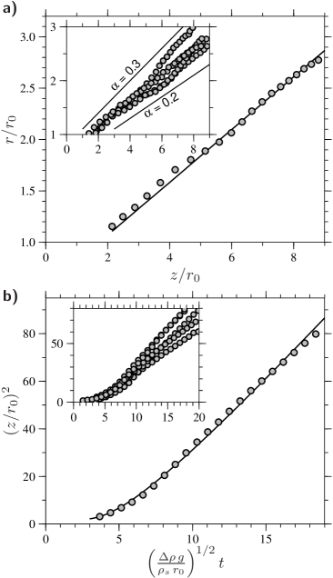
Figure 2: Time evolution of the mean radius and position of the falling fluid, in experiments where a volume of NaI solution is released into silicone oil ($\mathsf{P}=1.9$). a) Mean radius $r$ (normalized by $r_{0}$) of the aqueous solution/oil mixture as a function of the position $z$ (normalized by $r_{0}$) of its center of mass. b) Square of the normalized position $z$ of the center of mass of the aqueous solution/oil mixture as a function of time (normalized by $\left({\Delta\rho\,g}/{\rho_{s}\,r_{0}}\right)^{-1/2}$). The results of one experiment are compared with the predictions of our model based on the entrainment assumption shown with black lines in a) and b). For this experiment, the model [Eqs. (54), (55) and (56)] best fits the data with $\alpha=0.26$, a drag coefficient $C_{d}=0.53$, and a virtual mass coefficient $K=0.5$ (see B for details on the model). The experimental results shown in the inserts illustrate the natural variability seen in our experiments, with $\alpha$ varying between 0.2 and 0.3.

6   Fragmentation

Fig. 1b-c reveals that the dense NaI solution entrains and incorporates silicone oil before it fragments into droplets. Fragmentation occurs relatively late in the descent process (between the third and fourth pictures in the experiment shown in Fig. 1b-c), at a time when a sizable volume of ambient fluid has already been entrained. Droplets appear in a single global fragmentation event, which is at variance with previously suggested "cascade" processes, in which a succession of fragmentation events lead to the final stable drop size [Rubie et al., 2003; Samuel, 2012], and "erosion" processes, in which metal-silicate mixing occurs predominantly on the boundary with the ambient fluid [Dahl and Stevenson, 2010].

Adding a small amount of fluorescent dye to the NaI solution and illuminating the experiment with a thin light sheet reveals cross-sections of the NaI solution/silicone oil mixture, one example being shown in Fig. 3. Small scale mixing of the phases is evident in this picture, demonstrating that oil has been entrained into the NaI solution and that the two phases are already intimately mixed before fragmentation occurs. This striking observation suggests that fragmentation is a consequence of mixing associated with turbulent entrainment of the ambient fluid, with fragmentation into drops ultimately resulting from small scale instabilities, plausibly capillary instabilities developed on filaments stretched by the turbulent flow [Villermaux et al., 2004; Shinjo and Umemura, 2010].

Figure 3: Cross-section of the NaI solution/silicone oil mixture at a distance $\sim 2\,d_{0}$ from the origin. The experiment is illuminated with a thin light sheet exciting a fluorescent dye (Rhodamine B) added to the NaI solution, which appears white in the picture. In this experiment $Bo=4.6\times 10^{3}$, $W\!e=2\times 10^{3}$, $\mathsf{P}=1.54$, $\mathsf{H}=2.1$, and $Re=2\times 10^{4}$.

In all our experiments in this turbulent regime, fragmentation into drops is observed to occur after the dense liquid falls a distance equal to 3 to 4 times its initial diameter, with no clear trend observed in the explored range of parameters. At this point the volume fraction of the dense fluid in the mixture is of order 5-10 %. It is possible that the fragmentation distance becomes independent of $Re$ and $W\!e$ when these two numbers are large, but the maximum value of $W\!e$ obtained in our experiments (3000) is only 6 times larger than its observed critical value for this turbulent regime ($\sim 500$), making the explored range of $W\!e$ too small to test this possibility.

7   Chemical equilibration before fragmentation - a fractal model

Fragmentation of the metal phase into drops is an important facet of the problem of metal-silicate interactions, because drop formation is an efficient way of increasing the interfacial area between metal and silicate, thus enhancing chemical transfer and equilibration. However, it may not be necessary for chemical equilibration. The small scale mixing observed in our experiments (Fig. 3) results in a highly convoluted interface, which should drastically decrease the timescale of equilibration with the entrained silicate.

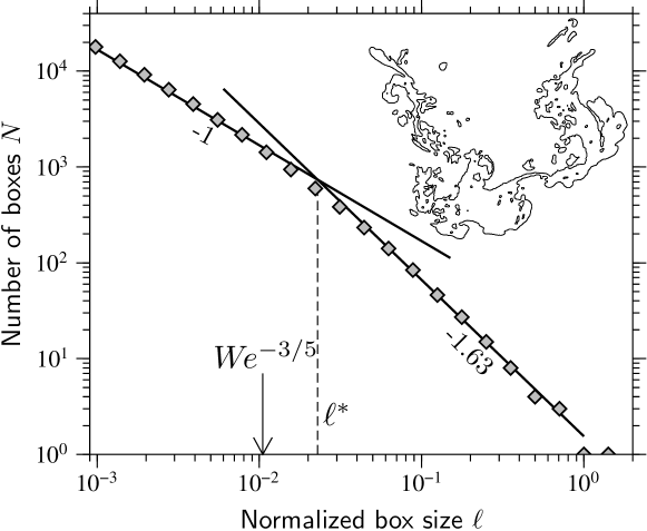
Figure 4: The fractal dimension of the oil/aqueous solution interface shown in Fig. 3, determined using a box counting algorithm. Shown here is the number $N(\ell)$ of square boxes of size $\ell$ required to cover the oil/aqueous solution interface as a function of the box size $\ell$. Here the box size $\ell$ is normalized by the size of the smallest box fully enclosing the interface. The slope of the resulting curve is $1-D$, where $D$ is the fractal dimension of the 3D interface. A slope of $-1$ is expected for a non-fractal surface, as found here for small $\ell$. The interface is fractal at scales above $\ell^{*}\simeq 2.3\times 10^{-2}$, which is of the same order of magnitude as $W\!e^{-{3}/{5}}\simeq 1.05\times 10^{-2}$. Fitting the data for $\ell>\ell^{*}$ (thick black line) gives a slope of $-1.63\pm 0.03$ ($\pm 1\,\sigma$), which implies a fractal dimension of $2.63\pm 0.03$, slightly smaller than $D=8/3=2.67$.

To illustrate this point, we consider a model of metal-silicate equilibration prior to drop formation based on the observation that the interface separating the two fluids has a fractal nature once turbulence is well-developed. Theory [Mandelbrot, 1975; Constantin et al., 1991; Constantin and Procaccia, 1994] and experiments [Sreenivasan et al., 1989; Constantin et al., 1991] show that isosurfaces of transported quantities (composition, temperature) in well-developed turbulent flows are fractal – a consequence of the self-similarity of the turbulent flow – with a fractal dimension predicted to be $D=8/3$ for homogeneous turbulence with Kolmogorov scaling.

It is to be expected that the interface between immiscible fluids in a turbulent flow shares this property over the range of scales in which interfacial tension is unimportant. Experimental support for this assumption is given in Fig. 4, where the interface between the oil and aqueous solution is shown to have a fractal nature with a fractal dimension at scales larger than a cut-off length $\ell^{*}$. For miscible fluids, Sreenivasan et al. [1989] assumed that the inner cut-off length is the Kolmogorov scale for isovorticity surfaces, and the Batchelor scale for isocompositional surfaces for high Schmidt number fluids. For a surface separating two immiscible fluids, we expect that the inner cut-off length will be the largest of the Kolmogorov scale $\ell_{K}=d\,Re^{-3/4}$ and the scale $\ell_{\sigma}=d\,W\!e^{-3/5}$ at which interfacial tension balances local dynamic pressure fluctuations estimated assuming a Kolmogorov cascade [[Kolmogorov, 1949; Hinze, 1955], and see section 8 for more details]. Typically $\ell_{\sigma}\gg\ell_{K}$, and we expect that $\ell^{*}\sim\ell_{\sigma}$. In our experiments, $\ell^{*}$ and $\ell_{\sigma}$ are numerically close (within a factor of 2, Fig. 4) and the measured fractal dimension is only slightly smaller than the theoretical value of $8/3$. Note that the observed fractal nature of the interface is indicative of self-similarity in the flow, and that the measured fractal dimension is consistent with Kolmogorov type turbulence and a $k^{-5/3}$ kinetic energy spectrum.

Assuming that the metal-silicate interface has a fractal nature offers a convenient way of estimating its area $A_{T}$, which according to fractal geometry is $A_{T}=A_{0}(\ell^{*}/d)^{2-D}$, where $A_{0}=\pi d^{2}$ is the area measured at the scale $d$. Using $\ell^{*}\sim\ell_{\sigma}$, the predicted surface area is $A_{T}\sim A_{0}W\!e^{\frac{3}{5}(D-2)}$. With $D=8/3$ and $W\!e=10^{14}$, this implies an increase in interfacial area by five orders of magnitude. A timescale for chemical equilibration, $\tau_{\mathrm{eq}}$, can then be found by coupling the estimate for $A_{T}$ with a local scaling for turbulent mass flux at the metal-silicate interface.

Figure 5: A sketch of the composition profiles in the vicinity of the metal-silicate interface. The situation depicted here is that of a siderophile element in excess in the silicate phase.

We denote by $\kappa_{c}$ the diffusivity of the chemical element of interest. The Schmidt number $S\!c=\nu/\kappa_{c}$, where $\nu$ is the kinematic viscosity, is assumed to be large in both phases. Fig. 5 shows a sketch of the composition profiles in the vicinity of the metal-silicate interface, with definitions of the main variables. Thermodynamic equilibrium is assumed at the metal/silicate interface, so that the concentrations by mass $c_{m}^{\mathrm{int}}$ and $c_{s}^{\mathrm{int}}$ at the interface are linked by the partition coefficient $D_{i}=c_{m}^{\mathrm{int}}/c_{s}^{\mathrm{int}}$, but the bulk compositions $\bar{c}_{m}$ and $\bar{c}_{s}$ are out of thermodynamic equilibrium, i.e. $\bar{c}_{m}/\bar{c}_{s}\neq D_{i}$. The resulting compositional boundary layers have thicknesses $\delta_{m,s}$, and we denote by $\Delta c_{m,s}$ the composition difference across the boundary layers. The local diffusive compositional flux across the interface scales as $\kappa_{c}\Delta c/\delta$ and the total mass flux $F\!_{c}$ is

$$F\!_{c}\sim\rho_{m}A_{T}\kappa_{c}^{m}\frac{\Delta c_{m}}{\delta_{m}}\sim\rho_{s}A_{T}\kappa_{c}^{s}\frac{\Delta c_{s}}{\delta_{s}}.$$ (7)

Continuity of the mass flux across the interface implies that the ratio $\gamma_{m/s}$ of $\Delta c_{m}$ to $\Delta c_{s}$ is

$$\gamma_{m/s}=\frac{\Delta c_{m}}{\Delta c_{s}}=\frac{\rho_{s}}{\rho_{m}}\frac{\kappa_{c}^{s}}{\kappa_{c}^{m}}\frac{\delta_{m}}{\delta_{s}}.$$ (8)

We now relate the compositional jumps $\Delta c_{s}$ and $\Delta c_{m}$ to the mean composition $\bar{c}_{m}$ and $\bar{c}_{s}$ of the metal and silicate phases. Using Eq. (8) together with the assumption of local thermodynamic equilibrium ($D_{i}=c_{m}^{\mathrm{int}}/c_{s}^{\mathrm{int}}$), we obtain the following expressions for $\Delta c_{s}$ and $\Delta c_{m}$ :

$$\Delta c_{s}=-\frac{\bar{c}_{m}-D_{i}\bar{c}_{s}}{\gamma_{m/s}+D_{i}},\quad\Delta c_{m}=-\gamma_{m/s}\frac{\bar{c}_{m}-D_{i}\bar{c}_{s}}{\gamma_{m/s}+D_{i}}.$$ (9)

Using $(\pi/6)\bar{\rho}\,d^{3}$ for the mass of the metal-silicate mixture, the evolution of composition in the metal and silicate phases are given by

$$\phi\frac{\pi}{6}\bar{\rho}\,d^{3}\frac{d\bar{c}_{m}}{dt} =-F\!_{c},$$ (10)

$$(1-\phi)\frac{\pi}{6}\bar{\rho}\,d^{3}\frac{d\bar{c}_{s}}{dt} =F\!_{c},$$ (11)

where $\phi$ is the mass fraction of the metal phase in the mixture. Combining Eqs. (10) and (11) and using the metal dilution $\Delta=(1-\phi)/\phi$, we obtain

$$\frac{d}{dt}\ln\left(\bar{c}_{m}-D_{i}\bar{c}_{s}\right)=-\frac{(1+\Delta)(D_{i}+\Delta)}{\Delta(D_{i}+\gamma_{m/s})}\frac{\rho_{s}}{\bar{\rho}}\,\frac{6\kappa_{c}^{s}}{d\,\delta_{s}}\,W\!e^{\frac{3}{5}(D-2)},$$ (12)

from which we obtain an equilibration timescale $\tau_{\mathrm{eq}}$ of order of magnitude given by

$$\tau_{\mathrm{eq}}=f(\Delta,D_{i},\gamma_{m/s})\,\frac{\bar{\rho}}{\rho_{s}}\,\frac{d\,\delta_{s}}{\kappa_{c}^{s}}\,W\!e^{-\frac{3}{5}(D-2)},$$ (13)

where the factor 6 in Eq. (12) has been omitted, on the basis that this expression for $\tau_{\mathrm{eq}}$ is based on an order of magnitude estimate of the flux across the interface [Eq. (7)], in which an unknown – presumably $\mathcal{O}(1)$ – factor has already been omitted. In Eq. (13), the function $f(\Delta,D_{i},\gamma_{m/s})$ is given by

$$f(\Delta,D_{i},\gamma_{m/s})=\frac{\Delta(D_{i}+\gamma_{m/s})}{(1+\Delta)(D_{i}+\Delta)}.$$ (14)

The function $f$ is $\mathcal{O}(1)$ for intermediate values of $\Delta$ (with a maximum always smaller than 1), but $f\rightarrow 0$ if $\Delta$ is small compared to $\min(1,D_{i})$ or large compared to $\max(1,D_{i})$.

We now estimate the boundary layers thicknesses $\delta$ in the metal and silicate phases (the subscript $m$ and $s$ will be omitted in what follows, with the understanding that the analysis applies to both phases). Denoting by $\ell$ the smallest scale of the flow in the vicinity of the interface, then the smallest scale $\delta$ of the compositional field is found by balancing the strain rate at scale $\ell$ with the diffusion rate at the scale $\delta$, i.e. $u_{\ell}/\ell\sim\kappa_{c}/{\delta}^{2}$. Assuming a Kolmogorov type velocity spectrum, the velocity at scale $\ell$ is $u_{\ell}\sim w(\ell/d)^{\frac{1}{3}}$, where $w$ is the large scale velocity. With these assumptions, we obtain

$$\delta=d\,{S\!c}^{-\frac{1}{2}}{Re}^{-\frac{1}{2}}\left(\frac{\ell}{d}\right)^{\frac{1}{3}}.$$ (15)

At this stage, further progress requires assumptions on the small scale structure of the turbulence in the vicinity of the metal-silicate interface :

1. If we assume that the turbulence structure is not affected by the presence of the interface and interfacial tension effects, then $\ell$ should be the Kolmogorov scale. Eq. (15) with $\ell=\ell_{K}=dRe^{-3/4}$ gives

   $$\delta=d\,S\!c^{-\frac{1}{2}}Re^{-3/4},$$ (16)

   which is the Batchelor scale $\ell_{B}$. With this estimate for $\delta$, we obtain

   $$\gamma_{m/s}=\left(\frac{\rho_{s}}{\rho_{m}}\right)^{5/4}\left(\frac{\kappa_{c}^{s}}{\kappa_{c}^{m}}\right)^{1/2}\left(\frac{\eta_{s}}{\eta_{m}}\right)^{1/4}$$ (17)

   and an equilibration timescale

   $$\tau_{\mathrm{eq}}=f(\Delta,D_{i},\gamma_{m/s})\,\frac{\bar{\rho}}{\rho_{s}}\,\frac{d^{2}}{\kappa_{c}^{s}}\,S\!c^{-1/2}Re^{-3/4}W\!e^{-\frac{3}{5}(D-2)}.$$ (18)

2. Alternatively, one might argue that the turbulent motion in the vicinity of the interface is damped by interfacial tension at scales smaller than $\ell_{\sigma}$. In this case the smallest scale of the flow is $\ell_{\sigma}\sim d\,W\!e^{-3/5}$ and the boundary layer thickness is

   $$\delta=d\,S\!c^{-\frac{1}{2}}Re^{-\frac{1}{2}}W\!e^{-\frac{1}{5}},$$ (19)

   which gives

   $$\gamma_{m/s}=\left(\frac{\rho_{s}}{\rho_{m}}\right)^{6/5}\left(\frac{\kappa_{c}^{s}}{\kappa_{c}^{m}}\right)^{1/2}$$ (20)

   and an equilibration timescale

   $$\tau_{\mathrm{eq}}=f(\Delta,D_{i},\gamma_{m/s})\,\frac{\bar{\rho}}{\rho_{s}}\,\frac{d^{2}}{\kappa_{c}^{s}}\,S\!c^{-\frac{1}{2}}Re^{-\frac{1}{2}}W\!e^{-\frac{3}{5}D+1}.$$ (21)

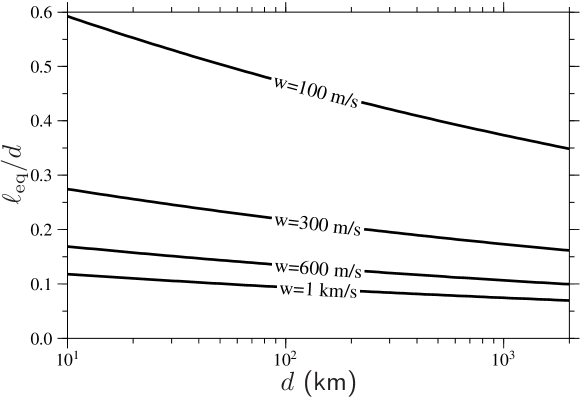
Figure 6: Equilibration distance $\ell_{\mathrm{eq}}/d$ as functions of the metal-silicate mixture diameter $d$, for $w=100,300,600$ and 1000 m.s^-1, calculated using Eq. (23) with $f(\Delta,D_{i})=0.5$, $\kappa_{c}^{s}\sim 10^{-8}$ m.s^-1, $\sigma=1$ J.m^-2 and $\rho_{s}=3500$ kg.m^-3.

Choosing between the two models Eqs. (18) or (21) would require detailed measurement of the small scale structure of the flow, or alternatively, measurements of a tracer concentration in both phases, which are beyond the scope of our current experimental set-up. We therefore choose the more conservative estimate of the equilibration timescale Eq. (21) which assumes that turbulent motions in the vicinity of the interface are damped at scales smaller than $\ell_{\sigma}$. For comparison, the model assuming no effect of the interface on the turbulence structure would yield an equilibration timescale a factor $W\!e^{1/5}Re^{-1/4}$ smaller (typically a factor of 5 or more smaller).

With $\rho_{s}/\rho_{m}\simeq 0.5$, assuming that $\kappa_{c}^{s}$ and $\kappa_{c}^{m}$ are of the same order of magnitude implies that $\gamma_{m/s}=\mathcal{O}(1)$. Since it only appears in $f(\Delta,D_{i},\gamma_{m/s})$ as a sum with $D_{i}$ which is $\gg 1$ for siderophile elements, the exact value of $\gamma_{m/s}$ should be of little importance. The factor ${\bar{\rho}}/{\rho_{s}}$ is also $\mathcal{O}(1)$, and ignoring it as well in Eq. (21) yields the simplified equilibration timescale

$$\tau_{\mathrm{eq}}=f(\Delta,D_{i})\,\frac{d^{2}}{\kappa_{c}^{s}}\,S\!c^{-\frac{1}{2}}Re^{-\frac{1}{2}}W\!e^{-\frac{3}{5}D+1}.$$ (22)

From Eq. (22), we obtain an equilibration distance $\ell_{\mathrm{eq}}=w\,\tau_{\mathrm{eq}}$ given by

$$\ell_{\mathrm{eq}}=f(\Delta,D_{i})\,d\,S\!c^{\frac{1}{2}}Re^{\frac{1}{2}}W\!e^{-\frac{3}{5}D+1},$$ (23)

which is the distance travelled by the metal phase during the time $\tau_{\mathrm{eq}}$ required for equilibration of the metal with the silicate it has mixed with. Metal and silicates equilibrate if the equilibration distance $\ell_{\mathrm{eq}}$ is smaller than the magma ocean depth. Fig. 6 shows $\ell_{\mathrm{eq}}$ as a function of $d$ for various values of $w$ between $100$ m.s^-1 and 1 km.s^-1, calculated with $f(\Delta,D_{i})=0.5$, $\kappa_{c}^{s}\sim 10^{-8}$ m.s^-1, $\sigma=1$ J.m^-2 and $\rho_{s}=3500$ kg.m^-3. The equilibration distance is always a fraction of the metal-silicate mixture diameter, and is usually smaller than plausible magma ocean depths.

8   Prediction for the stable drop size after fragmentation

After fragmentation, the metal-silicate equilibration timescale depends mostly on the resulting fragments size [Karato and Murthy, 1997; Rubie et al., 2003; Ulvrová et al., 2011]. In this section, we propose a scaling for the drop size of the metal phase after fragmentation, as well as a justification for the scaling used in the previous section for the cut-off length scale $\ell^{*}$ above which the interface (before fragmentation) is fractal. In a fully turbulent flow, the stable drop size $d_{d}$ after fragmentation, as well as the cut-off length scale $\ell^{*}$ before fragmentation, are expected to depend only on the dissipation rate $\epsilon$, the interfacial tension $\sigma$, the densities and viscosities of both phases, and the metal volume fraction :

$${\color[rgb]{0,0,0}(d_{d},}\ell^{*}{\color[rgb]{0,0,0})}=\mathcal{F}_{1}(\epsilon,\sigma,\rho_{m},\rho_{s},\nu_{s},\nu_{m},\phi).$$ (24)

Using the Vashy-Buckingham theorem, we find that $\ell^{*}$ must be the solution of an equation of the form

$$\mathcal{F}_{2}\left[\mathsf{P},\mathsf{H},\phi,\frac{\ell^{*}}{\ell_{K}},\frac{\ell^{*}}{\ell_{\sigma}}\right]=0.$$ (25)

where we have introduced two length scales,

$$\ell_{K}=\left(\frac{\nu_{s}^{3}}{\epsilon}\right)^{1/4},\quad\ell_{\sigma}=\left(\frac{\sigma}{\rho_{s}}\right)^{3/5}\epsilon^{-2/5}.$$ (26)

$\ell_{K}$ is the Kolmogorov scale, at which turbulent kinetic energy is dissipated into heat by the action of viscous forces; $\ell_{\sigma}$ can be shown to be the length scale at which interfacial tension (Laplace pressure) balances turbulent pressure fluctuations and stresses if a Kolmogorov type turbulence is assumed [Kolmogorov, 1949; Hinze, 1955]. With $\epsilon\sim w^{3}/r$ [Tennekes and Lumley, 1972],

$$\ell_{K}\sim Re^{-3/4}d,\quad\ell_{\sigma}\sim W\!e^{-3/5}d.$$ (27)

Two end-member cases are possible, depending on the relative values of $\ell_{K}$ and $\ell_{\sigma}$. Let us first compare the magnitude of the viscous stress and Laplace pressure at a given scale $\ell$. Assuming a Kolmogorov type turbulence cascade, the velocity fluctuations $u_{\ell}$ at scale $\ell$ is $u_{\ell}\sim w\left(\ell/d\right)^{1/3}$. Using this estimate for $u_{\ell}$, we find that the ratio of the viscous stress to the Laplace pressure at the scale $\ell$ is

$$\frac{\text{Viscous stress at scale }\ell}{\text{Laplace pressure at scale }\ell}\sim\frac{\eta_{s}u_{\ell}/\ell}{\sigma/\ell}\sim\left(\frac{\ell_{K}}{\ell_{\sigma}}\right)^{4/3}\left(\frac{\ell}{\ell_{\sigma}}\right)^{1/3}.$$ (28)

Two options are possible :

1. First, if $\ell_{K}\gg\ell_{\sigma}$, all the energy input is dissipated at the Kolmogorov scale, at which scale the ratio of viscous stress and Laplace pressure is $\sim(\ell_{K}/\ell_{\sigma})^{5/3}\gg 1$ according to Eq. (28). In this case interfacial tension is unimportant, and $d_{d}$ and $\ell^{*}$ scales as

   $${\color[rgb]{0,0,0}(d_{d},}\ell^{*}{\color[rgb]{0,0,0})}=\mathcal{F}_{3}\!\left(\mathsf{P},\mathsf{H},\phi\right)\left(\frac{\nu_{s}^{3}}{\epsilon}\right)^{1/4}\sim\mathcal{F}_{3}\!\left(\mathsf{P},\mathsf{H},\phi\right)d\,Re^{-3/4}.$$ (29)

2. Alternatively, if $\ell_{K}\ll\ell_{\sigma}$, then interfacial tension balances turbulent pressure and stress fluctuations at the scale $\ell_{\sigma}$, with further smaller scale deformation of the interface inhibited by the interfacial tension. According to Eq. (28), the ratio of viscous stress and Laplace pressure is $\sim(\ell_{K}/\ell_{\sigma})^{4/3}\ll 1$ at this scale, which implies that viscous effects are unimportant. As a consequence, the stable drop size does not depend on the viscosity of either phase, nor on the viscosity ratio $\mathsf{H}$, and thus the drop size and the cut-off length scale follow a scaling law of the form:

   $${\color[rgb]{0,0,0}(d_{d},}\ell^{*}{\color[rgb]{0,0,0})}=\mathcal{F}_{4}\!\left(\mathsf{P},\phi\right)\left(\frac{\sigma}{\rho_{s}}\right)^{3/5}\epsilon^{-2/5}\sim\mathcal{F}_{4}\!\left(\mathsf{P},\phi\right)d\,W\!e^{-3/5}.$$ (30)

The ratio ${\ell_{K}}/{\ell_{\sigma}}\sim W\!e^{3/5}Re^{-3/4}$ following an impact is found to be typically smaller than $10^{-2}$, which suggests that the drop size or cut-off length will be set by interfacial tension rather than viscosity, and will obey the scaling given by Eq. (30). When $\phi$ is small, its effect should be negligible, as indeed observed in experiments with dilute dispersions [Hinze, 1955; Chen and Middleman, 1967].

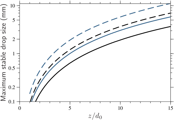
Figure 7: Maximum stable drop size after fragmentation according to Eq. (34), as a function of the distance travelled (normalized by the initial metal blob diameter $d_{0}$), for metal blobs with initial diameter 100 km (blue curves) and 1000 km (black curves) with $f=0.5$ (solid curves) and $f=0.1$ (dashed curves). Assumed parameters values are : $\alpha=0.25$, $K+{3\,C_{d}}/{16\,\alpha}=1$, $\Delta\rho=4000$ kg m^-3, $\rho_{s}=3500$ kg m^-3, $g=5$ m s^-2, $\sigma=1$ J m^-2.

From analysis of Clay [1940]’s data, Hinze [1955] found that the maximum drop size $d_{\mathrm{max}}$ in a turbulent flow with $\ell_{\sigma}\gg\ell_{K}$ is given by

$$d_{\mathrm{max}}\simeq 0.725\,\left(\frac{\sigma}{\rho_{s}}\right)^{3/5}\epsilon^{-2/5}.$$ (31)

Effects of changing the density ratio was not investigated in this study, which focused on fluids with density ratios $\mathsf{P}\simeq 1$. Theory [Levich, 1962] and experiments [Hesketh et al., 1987] argue for a dependence on the density ratio of the form $d_{\mathrm{max}}\propto\mathsf{P}^{-1/5}$. For the metal-silicate system, which has $\mathsf{P}\simeq 2$, this would predict a maximum drop size about $13$ % smaller than what Eq. (31) predicts, a minor discrepancy in light of the other uncertainties.

Clearly, the size of the drops produced by fragmentation of the metal blob must depend on the details of the fragmentation mechanism, which are not elucidated yet, and the drop size just after fragmentation does not have to match the prediction of Eq. (31) (although a similar scaling is expected). Nevertheless, Eq. (31) should give a reasonable upper bound for the fragment size, since it predicts that larger drops would be disrupted by turbulent dynamic pressure fluctuations.

In a system in statistical steady state, the dissipation rate $\epsilon$ must equal the total energy input in the system $e_{\mathrm{in}}$, which here is the rate of work of the buoyancy forces. However, since the metal-silicate mixture is not in statistical steady state (it can be shown using the self-similar regime velocity (Eq. (4)) that the total kinetic energy of the system evolves with time), dissipation does not equal the rate of energy input, but is some fraction $f$ of the work done by the buoyancy forces. The rate of work of the buoyancy forces,

$$e_{\mathrm{in}}=\bar{\phi}\,\frac{\Delta\rho}{\bar{\rho}}\,g\,w,$$ (32)

tends towards

$$e_{\mathrm{in}}=2\left[1+K+\frac{3}{16}\frac{C_{d}}{\alpha}\right]^{-1/2}\frac{\rho_{s}}{\bar{\rho}}\left[\frac{\Delta\rho\,g\,r_{0}^{1/3}}{2\alpha^{3}\rho_{s}}\right]^{3/2}\left(\frac{r_{0}}{z}\right)^{4},$$ (33)

in the self-similar regime, for which $w$ is given by Eq. (4). Using Eq. (33) for $e_{\mathrm{in}}$ and writing the dissipation as $\epsilon=f\,e_{\mathrm{in}}$, we find that

$$\frac{d_{\mathrm{max}}}{d_{0}}\simeq\frac{3}{f^{2/5}}\left[1+K+\frac{3}{16}\frac{C_{d}}{\alpha}\right]^{1/5}\left(\frac{\bar{\rho}}{\rho_{s}}\right)^{2/5}\frac{\alpha^{9/5}}{Bo_{0}^{3/5}}\left(\frac{z}{d_{0}}\right)^{8/5}$$ (34)

when the mixture has reached the self-similar regime. Here $Bo_{0}=\Delta\rho\,g\,d_{0}^{2}/\sigma$. The value of $f$ is difficult to estimate precisely, but shouldn’t be much smaller than 1. Fig. 7 shows $d_{\mathrm{max}}$ from Eq. (34) for metal blobs with initial diameter 100 km (blue curves) and 1000 km (black curves) with $f=0.5$ (solid curves) and $f=0.1$ (dashed curves), and $\alpha=0.25$. Smaller values of $\alpha$ would result in smaller drop sizes. Eq. (34) predicts submillimeter-to-centimeter maximum stable drop sizes, which is small enough to ensure fast re-equilibration with the surrounding silicates [Karato and Murthy, 1997; Rubie et al., 2003; Ulvrová et al., 2011].

9   Discussion

9.1   On the relevance of our experiments for the core formation problem

Uncertainties about the applicability of our results to metal-silicate mixing and fragmentation in magma oceans are due mostly to the fact that our experiments are still very far from the impact conditions with $Re$, $We$ and $Bo$ up to ten orders of magnitude smaller than during Earth accretion. The main obstacles to improving experimental as well as numerical approaches stem from the three dimensional, turbulent nature of the flow at these extreme parameters. Direct numerical simulations of turbulent flows at such high Re are prohibitively expensive. For example, the cost of a direct numerical simulation resolving the Kolmogorov scale goes as $\sim Re^{11/4}$, which implies that increasing $Re$ by a factor of 10 multiplies the cost by about 500.

Accordingly, a legitimate question is : how close to the dynamical conditions of accretion do we need to go ? In boundary free turbulent flows involving fully miscible fluids, it is observed that there is no qualitative change of the flow associated with increasing $Re$ once turbulence is "fully-developed", i.e. once there is a range of length scales (the inertial range) for which viscosity effects are negligible [e.g. Mungal and Hollingsworth, 1989]. Increasing $Re$ further increases the gap between the integral scale (the largest scale of the flow, here the diameter of the blob) and the Kolmogorov scale at which viscous dissipation occurs, but does not change the slope of the kinetic energy spectrum. The entrainment coefficient in turbulent thermals appears to be independent of $Re$ [e.g. Turner, 1969] once $Re\gtrsim 10^{3}$, which is consistent with the rate of turbulent entrainment being controlled by the largest, inviscid eddies [Turner, 1986].

In immiscible fluid systems like metal-silicate, we should expect that a similar asymptotic regime is reached once there is a separation of scales between the integral scale of the flow and the Kolmogorov ($d\,Re^{-3/4}$) and capillary ($d\,W\!e^{-3/5}$) scales, so that there is a range of scales for which viscosity and interfacial tension do not play any role. Increasing further $Re$ and $W\!e$ will increase the ratio between the largest and smallest scales of the flow, but should not change the phenomenology, nor the slope of the kinetic energy spectrum in the inertial range. By analogy with the miscible fluid case, the entrainment coefficient in the immiscible fluids case should not depend on $W\!e$ and $Re$ once these numbers are large enough.

While it is difficult to demonstrate without heavier instrumentation and actual velocity measurements that our experiments have indeed reached a large $Re$, large $W\!e$ asymptotic regime, there are a number of observations which are consistent with our experiments being at least close to such regime: (i) the measured coefficient of entrainment is similar to that measured in miscible turbulent thermals, consistent with the entrainment rate being independent of the interfacial tension; (ii) the observed fractal nature of the interface is indicative of self-similarity in the flow, and the measured fractal dimension is consistent with a $k^{-5/3}$ spectrum; (iii) the cut-off length observed in cross-sections of the mixture, which presumably corresponds to the capillary scale, is more than a decade smaller than the diameter of the NaI-silicon oil mixture (40 times smaller in Fig. 4).

Together, these observations support our claim that the entrainment model, and the entrainment coefficient value of $\simeq 0.25$ which we observe, should indeed apply to larger values of $Re$ and $W\!e$. However, there is one more point which needs to be discussed : compressibility effects, which are absent in our experiments (the Mach number $M$ is $\sim 10^{-4}$), may be significant in the flow following an impact, which can often be supersonic. This is probably the most severe limitation of our experiments. The fact that the flow velocity is similar to the sound velocity has an important qualitative consequence for the structure of the flow: the finite speed of sound introduces a time delay in the transmission of pressure signals from one point to another, which makes impossible for large turbulent eddies to remain coherent when the local Mach number (based on the eddy velocity scale) is of order one or larger [Breidenthal, 1992; Freund et al., 2000; Pantano and Sarkar, 2002]. Because the rate of entrainment is thought to be controlled by the process of engulfment of ambient fluid by large scale eddies [Brown and Roshko, 1974; Turner, 1986; Mathew and Basu, 2002], mixing is expected to decrease when ${M}$ approaches $1$. Experiments on compressible turbulent jets and mixing layers show that the entrainment rate indeed decreases significantly with increasing $M$, before saturating at a value about five times smaller than for incompressible flows [Brown and Roshko, 1974; Freund et al., 2000] when $M\gtrsim 1$. An entrainment coefficient several times smaller than the $0.25\pm 0.05$ value of our experiments might therefore be expected when the Mach number of the metal-silicate mixture is $\mathcal{O}(1)$.

9.2   Comparison with previous work

The reduction of a large metal blob to a drop size has been investigated by Dahl and Stevenson [2010] and Samuel [2012]. Two different scenarios have been considered by Dahl and Stevenson [2010]. In a first model, metal-silicate mixing is assumed to occur through gradual erosion of the metal blobs by small scale Rayleigh-Taylor instabilities. The model predicts that only relatively small metal blobs (less than 10 km in diameter) efficiently mix with silicates, larger blobs reaching the core of the growing planet without significant chemical interactions with the surrounding silicates. In a second model, Dahl and Stevenson [2010] considered the possibility of metal-silicate mixing through turbulent entrainment, similar to the model we present here, but their analysis of the structure of the turbulence lead them to conclude that mixing associated with the entrainment process does not proceed to length scales small enough to permit efficient chemical re-equilibration. Our experiments suggest that mixing does proceed down to the capillary scale at which surface tension balances dynamic pressure fluctuations, and our model for the kinetics of equilibration predicts fast re-equilibration, implying that the metal should continuously equilibrate with the entrained silicates once turbulence is well-developed. However, remember that fast equilibration between the metal and entrained silicates does not necessarily imply a significant flux of elements from one phase to the other, because this also depends on the amount of metal-silicate mixing. Although the entrainment model predicts significantly more mixing than the Rayleigh-Taylor erosion model of Dahl and Stevenson [2010], chemical re-equilibration remains problematic for the largest impacts (see further discussion in section 10).

Numerical models of the evolution of a metal blob falling in molten silicates by Samuel [2012] indicate metal fragmentation occurs through a sequence of events leading to the final stable drop size, that are quite different from our experimental results. In our view, a major limitation of the Samuel [2012] study is the assumption of axisymmetry of the flow, a constraint that inhibits the development of turbulence.

Regarding the size of the fragments resulting from the metal fragmentation process, models for the maximal stable drop size have been discussed by Stevenson [1990], Karato and Murthy [1997], and Rubie et al. [2003]. Although we argue for a different scaling for the stable drop size (section 8), the implications are essentially the same : if the metal phase is fragmented down to the stable drop size, then this size is small enough for ensuring fast chemical re-equilibration between the drops and surrounding silicates.

10   Implications for planetary core formation

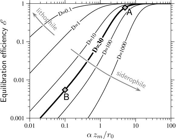
Figure 8: Equilibration efficiency $\mathscr{E}_{i}$ as a function of $\alpha z_{m}/r_{0}$ (where $z_{m}$ is the depth of the magma ocean) and various values of the partition coefficient $D$, estimated for metal-silicate mixing in a magma ocean as predicted by the turbulent entrainment model (Eq. (6)). Point $\mathsf{A}$ corresponds to the case of a metal blob falling through a magma ocean of depth ten times its diameter, with $\alpha=0.25$. Point $\mathsf{B}$ corresponds to the case of a giant impact with $r_{0}=0.5\,z_{m}$ and $\alpha=0.05$.

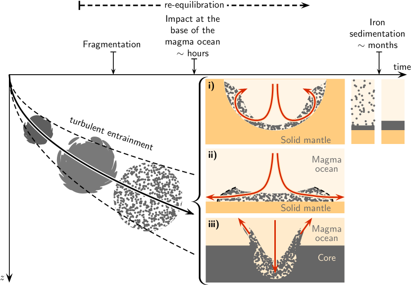
Figure 9: Possible scenarios for metal-silicate mixing and segregation following a large impact involving a previously differentiated impactor. The metal is shown in grey, molten silicate in light orange, and solid silicate in dark orange. The metal phase gradually mixes with the silicates through turbulent entrainment, with efficient chemical equilibration resulting from small-scale mixing. Additional mixing may be caused by the impact of the metal-silicate mixture at the base of the magma ocean.

As shown in the introduction section [see Eq. (1)], efficient chemical re-equilibration requires that two necessary conditions are met : (i) that the metal phase is capable of equilibrating with the silicates it has mixed with (i.e. that the parameter $k$ in Eq. (1) is of order 1), and (ii) that the metal phase equilibrates with a silicate mass at least a factor $D_{i}$ larger (i.e. that the metal dilution $\Delta\gtrsim D_{i}$).

With a velocity $w$ in the range 0.1-1 km.s^-1 and diameter $d>10$ km, our model predicts that the equilibration distance $\ell_{\mathrm{eq}}$ (the distance travelled by the metal phase during the time needed for equilibration) is always smaller than about $0.6\,d$ (Fig. 6). For example, Eq. (23) yields $\ell_{\mathrm{eq}}\simeq 50$ km for $d=100$ km and $w=100$ m.s^-1, and $\ell_{\mathrm{eq}}\simeq 75$ km for $d=1000$ km and $w=1$ km.s^-1, assuming $\kappa_{c}=10^{-8}$ m².s^-1, $\rho_{s}=3500$ kg.m^-3, $\sigma=1$ J.m^-2, and $f(\Delta,D_{i})=0.5$. The corresponding equilibration timescales are $\tau_{\mathrm{eq}}\simeq 8$ min and $\simeq 75$ s, respectively. Since $\ell_{\mathrm{eq}}$ is smaller than the metal-silicate mixture diameter, and small compared with the typical depth of a magma ocean, the metal phase and the entrained silicate should readily equilibrate once turbulence is fully developed, which typically requires one advection time $\sim d/w$, or a distance of fall $\sim d$. Re-equilibration should be efficient as well once the metal phase is fragmented : the maximum stable size of the resulting fragments is expected to scale as $d\,W\!e^{-3/5}$ [Kolmogorov, 1949; Hinze, 1955; Risso, 2000], which predicts submillimeter-to-centimeter size drops, small enough for fast re-equilibration [Karato and Murthy, 1997; Rubie et al., 2003; Ulvrová et al., 2011]. This suggests that once turbulence is well-developed, most of the metal indeed equilibrates with the surrounding silicates and $k$ should be close to 1. Whether or not metal-silicate equilibration has a significant geochemical fingerprint then depends on the ratio $\Delta/D_{i}$. Assuming that metal-silicate mixing occurs through turbulent entrainment, Fig. 8 shows that the equilibration efficiency $\mathscr{E}_{i}$, calculated using Eqs. (1) and (6) with $k=1$, depends strongly on the quantity $\alpha\,z_{m}/r_{0}$, where $z_{m}$ is the depth of the magma ocean.

The above considerations suggest that efficient metal-silicate equilibration should have been the norm for impacts in which the magma ocean is much deeper than the impactor core diameter. As an example, Eq. (6) predicts that a molten iron blob falling through a magma ocean of depth ten times its diameter mixes with about 100 times its mass of silicate, assuming $\alpha=0.25$ (a relevant value here because the large value of $z_{m}/r_{0}$ ensures deceleration of the metal phase to subsonic velocity, irrespectively of the initial conditions). The large value of $z_{m}/r_{0}$ also ensures well-developed turbulence and fast equilibration. The resulting Tungsten equilibration efficiency is $\mathscr{E}_{W}\simeq 0.78$ (point $\mathsf{A}$ in Fig. 8), assuming $D_{W}=30$.

The cases of impacts for which $z_{m}/r_{0}$ is not much larger than one, which includes the Moon-forming event, are not as clear. First, it is not obvious that the time needed for the impactor core material to reach the base of the magma ocean would allow enough turbulence to develop and the metal-silicate interfacial area to increase sufficiently for fast equilibration. Second, and as discussed in section 9.1, the effect of compressibility on $\alpha$ may significantly reduce the entrainment rate, allowing only a small mass of silicate to mix with the metal. Assuming, as for turbulent jets, a fivefold decrease of the entrainment rate due to compressibility, $\alpha=0.25/5=0.05$, the core of an impactor with $\simeq 10$% the mass of the proto-Earth ($r_{0}\simeq 0.5\,z_{m}$) would mix with only about 17 % its mass of silicate before it reaches the proto-Earth’s core, giving $\mathscr{E}_{W}\simeq 5.5\ 10^{-3}$ (point $\mathsf{B}$ in Fig. 8). However, the actual equilibration efficiency may depend on the details of the impact dynamics. SPH simulations of the Moon-forming impact suggest that in the likely case of an oblique impact, a fraction of the impactor including most of its core would be sheared past the planet before re-impacting Earth’s mantle [Canup, 2004]. Some degree of disruption of the impactor core during this process might be sufficient to allow subsequent metal-silicate equilibration by increasing the value of $\alpha\,z_{m}/r_{0}$ for individual blobs.

Lastly, we point out that core-mantle segregation is a complex, multi-step process and additional equilibration is possible at other stages. In particular, the velocity of the metal-silicate mixture may easily exceed hundreds of m.s^-1, implying an energetic "secondary impact" when it reaches the bottom of the magma ocean, which, as sketched in Fig. 9, could cause significant additional metal-silicate mixing [Deguen et al., 2011]. (i) In the case of an impact forming its own semi-spherical magma pool, the inertia of the mixture can drive an upward flow, re-suspending iron fragments [Deguen et al., 2011] which, in spite of likely vigorous convection, sediment out on a timescale similar to the Stokes’ sedimentation time [Martin and Nokes, 1988; Lavorel and Le Bars, 2009]. (ii) In a pre-existing global magma ocean with a horizontal lower boundary, the metal-silicate mixture will rather spread laterally as a turbulent gravity current - analogous to a pyroclastic flow - with possibly significant additional entrainment of molten silicate [Hallworth et al., 1993]. (iii) If the mantle is fully molten, the metal-silicate mixture directly impacts the proto-Earth’s core, with splashing and entrainment of mantle material into the core [Storr and Behnia, 1999] providing additional metal-silicate mixing.

Acknowledgement

We would like to thank H. J. Melosh, David Rubie, and an anonymous reviewer for helpful comments and suggestions. This research was supported by NSF grants EAR-110371 and EAR-1135382 (FESD).

Appendix A Equilibration efficiency

Definition

Let $c_{m}$ and $c_{s}$ denote the concentrations (in weight %) of element $i$ in either the metal or silicate phases, respectively. The metal and silicate are fully equilibrated when the two phases have reached thermodynamic equilibrium, for which the equilibrium concentration $c_{m}^{\mathrm{eq}}$ and $c_{s}^{\mathrm{eq}}$ are linked through the metal/silicate partition coefficient $D_{i}$ by $c_{m}^{\mathrm{eq}}=D_{i}\,c_{s}^{\mathrm{eq}}$.

Consider a mass $M_{m}$ of metal, in which we assume that a fraction $k\,M_{m}$ has been mixed and equilibrated with a mass $M_{s}$ of silicates. We define the metal dilution $\Delta$ as the ratio of the mass of equilibrated silicate over the mass of equilibrated metal,

$$\Delta=\frac{M_{s}}{kM_{m}}.$$ (35)

Given initial values $c_{m}^{0}$ and $c_{s}^{0}$ of the concentration in the metal and silicate phases, the concentration in the equilibrated metal $c_{m}^{\mathrm{eq}}$ and equilibrated silicate $c_{s}^{\mathrm{eq}}$ are found from mass conservation,

$$c_{m}^{\mathrm{eq}}+\Delta\,c_{s}^{\mathrm{eq}}=c_{m}^{0}+\Delta\,c_{s}^{0},$$ (36)

which, together with the assumption of thermodynamic equilibrium, $c_{m}^{\mathrm{eq}}=D_{i}\,c_{s}^{\mathrm{eq}}$, gives

$$c_{m}^{\mathrm{eq}}=\frac{c_{m}^{0}+\Delta\,c_{s}^{0}}{1+\Delta/D_{i}},\quad c_{s}^{\mathrm{eq}}=\frac{c_{m}^{0}+\Delta\,c_{s}^{0}}{D_{i}+\Delta}.$$ (37)

The net mass exchange $\mathcal{M}_{i}$ of element $i$ between the metal and silicate phases can be written as

$$\mathcal{M}_{i} =k\,M_{m}|c_{m}^{\mathrm{eq}}-c_{m}^{0}|=M_{s}|c_{s}^{\mathrm{eq}}-c_{s}^{0}|$$ (38)

$$=k\,M_{m}\frac{|c_{m}^{0}-D_{i}c_{s}^{0}|}{1+D_{i}/\Delta}.$$ (39)

$\mathcal{M}_{i}$ reaches a maximum value $\mathcal{M}_{i}^{\mathrm{max}}=M_{m}|c_{m}^{0}-D_{i}c_{s}^{0}|$ when all the metal phase is equilibrated ($k=1$) and is infinitally diluted in the silicate phase ($\Delta\rightarrow\infty$). We thus define the equilibration efficiency $\mathscr{E}_{i}$ of element $i$ as the actual mass exchange $\mathcal{M}_{i}$ normalized by the maximum possible mass exchange $\mathcal{M}_{i}^{\mathrm{max}}$. From Eq. (39) and the value of $\mathcal{M}_{i}^{\mathrm{max}}$, the equilibration efficiency is found to be

$$\mathscr{E}_{i}=\frac{k}{1+D_{i}/\Delta},$$ (40)

which reduces to $k$ when $\Delta/D_{i}\gg 1$, the limit that is usually assumed in continuous accretion models [e.g. Rudge et al., 2010].

As shown by Eq. (40), the equilibration efficiency $\mathscr{E}_{i}$ depends critically on the ratio $\Delta/D_{i}$, and is small, even when $k=1$, if $\Delta$ is small compared to $D_{i}$. Efficient re-equilibration requires the metal dilution to be similar to or larger than the partition coefficient of the element considered. For Tungsten, which has $D_{W}\simeq 30$, efficient re-equilibration thus requires that the metal re-equilibrates with at least $30$ times its mass of silicate.

Use of $\mathscr{E}_{i}$ in geochemical models

We demonstrate here that geochemical models assuming partial equilibration of the metal phase but infinite dilution can be generalized by using the equilibration efficiency $\mathscr{E}_{i}$ in place of $k$. We consider the case of continuous accretion, according to the formulation of Rudge et al. [2010] (see their Supplementary Information). Discontinuous accretion can be treated in the same way.

We note $c_{m}(t)$ and $c_{s}(t)$ the concentration in Earth’s mantle and core at time $t$, and $c_{m}^{\mathrm{imp}}(t)$ and $c_{s}^{\mathrm{imp}}(t)$ the composition of the metal and silicate phase of the impacting bodies. The mass of the Earth is denoted by $M(t)$, and, using $F$ for the mass fraction of metal in the Earth (assumed constant), then the masses of the core and mantle are $FM(t)$ and $(1-F)M(t)$, respectively. We assume for simplicity that all impactors have the same metal mass fraction $F$.

Conservation of mass of element $i$ in Earth’s core implies that

$$\frac{d}{dt}\left[FMc_{m}\right]=\underbrace{(1-k)Fc_{m}^{\mathrm{imp}}\frac{dM}{dt}}_{\text{Flux of non-equilibrated metal}}+\underbrace{kFc_{m}^{\mathrm{eq}}\frac{dM}{dt}}_{\text{Flux of equilibrated metal}}$$ (41)

where $c_{m}^{\mathrm{eq}}$ is the concentration in the re-equilibrated fraction of the impactor core. One complication is that the metal of the impactor may equilibrate with silicates from both the impactor mantle and Earth’s mantle, in unknown proportion. If $\tilde{c}_{s}$ denotes the mean composition of the equilibrated silicate, Eq. (37) yields

$$c_{m}^{\mathrm{eq}}=\frac{c_{m}^{\mathrm{imp}}+\Delta\,\tilde{c}_{s}}{1+\Delta/D_{i}}.$$ (42)

For siderophile elements such as Tungsten, $\tilde{c}_{s}$ can be approximated by $c_{s}(t)$. As discussed above in A, the effect of re-equilibration is significant only if the metal re-equilibrates with a mass of silicates about $D_{i}$ times larger (e.g. about 30 times larger for Tunsten). Since the mass of the impactor mantle is only about twice the mass of its core, efficient re-equilibration of siderophile elements requires that the impactor metal equilibrates with a mass of Earth’s mantle significantly larger than the impactor’s mantle. This implies that, in cases where equilibration is efficient, the mean concentration of the equilibrated silicate is close to $c_{s}(t)$. The approximation $\tilde{c}_{s}\simeq c_{s}(t)$ is not valid if the equilibration efficiency is small, but in that situation it has little effect on the results.

Substituting Eq. (42) into Eq. (41) yields the following equation for the compositional evolution of the core :

$$\frac{d}{dt}\left(Mc_{m}\right)=\left[\mathscr{E}_{i}D_{i}\tilde{c}_{s}+(1-\mathscr{E}_{i})c_{m}^{\mathrm{imp}}\right]\frac{dM}{dt},$$ (43)

while conservation of element $i$ in the mantle yields the following equation for the mantle :

$$\frac{d}{dt}\left(Mc_{s}\right)=\left[c_{s}^{\mathrm{imp}}+\mathscr{E}_{i}\frac{F}{1-F}(c_{m}^{\mathrm{imp}}-D_{i}\tilde{c}_{s})\right]\frac{dM}{dt}.$$ (44)

If $\tilde{c}_{s}$ is taken to be equal to $c_{s}(t)$, equations (43) and (44) are the same as used by Rudge et al. [2010] for stable species if $\mathscr{E}_{i}$ is substituted for $k$ (see their equations A.3 and A.4 in the Supplementary Information). The equivalence also holds if radioactive or radiogenic species are considered (see the Supplementary Information of Rudge et al. [2010] for a detailed derivation of the relevant equations). Results of previous accretion models, including the bounds on Earth’s accretion derived by Rudge et al. [2010] from Hf-W and U-Pb systematics, can therefore be generalized to include the effect of finite dilution by using $\mathscr{E}_{i}$ in place of $k$.

Implications

Previous studies [Kleine et al., 2004; Nimmo et al., 2010; Rudge et al., 2010] have shown that Hf-W systematics can be used to infer a lower bound for the mean degree of re-equilibration during Earth’s accretion. Assuming infinite dilution of the metal phase, [Rudge et al., 2010] found that Hf-W systematics constrains the fraction of equilibrated metal $k$ to be larger than about 0.36 on average during Earth’s accretion. If finite metal dilution is considered, the implication is that $\mathscr{E}_{W}\geq\mathscr{E}_{W}^{\mathrm{min}}=0.36$, which requires that $k>0.36$ and, assuming $D_{W}\simeq 30$, $\Delta\geq\Delta^{\mathrm{min}}={D_{W}}/({1/\mathscr{E}_{W}^{\mathrm{min}}-1})\simeq 17$.

A possibly important implication for modeling the abundance of siderophile elements in the mantle is that the equilibration efficiency $\mathscr{E}_{i}$ is element-dependent. One consequence is that constraints on the equilibration efficiency from Hf-W systematics do not apply directly to other elements. The equilibration efficiency of an element $i$ with partition coefficient $D_{i}$ differs from the Tungsten equilibration efficiency $\mathscr{E}_{W}$ according to

$$\mathscr{E}_{i}=g(D_{W},D_{i},\Delta)\,\mathscr{E}_{W},$$ (45)

where

$$g(D_{W},D_{i},\Delta)=\frac{1+D_{W}/\Delta}{1+D_{i}/\Delta}.$$

In Eq. (45), the function $g$ is an increasing function of $\Delta$ if $D_{i}>D_{W}$, and a decreasing function of $\Delta$ if $D_{i}<D_{W}$. Thus the lower bounds on $k$ and $\Delta$ deduced from Hf-W systematics imply the following lower bound on the equilibration efficiency of an element $i$ :

$$\mathscr{E}_{i}\geq\mathscr{E}_{i}^{\mathrm{min}}=\begin{cases}\frac{1+D_{W}/\Delta^{\mathrm{min}}}{1+D_{i}/\Delta^{\mathrm{min}}}\mathscr{E}_{W}^{\mathrm{min}}&\text{if}\ D_{i}\geq D_{W},\\ \mathscr{E}_{W}^{\mathrm{min}}&\text{if}\ D_{i}\leq D_{W}.\end{cases}$$ (46)

The constraint on the equilibration efficiency becomes weaker for elements that are more siderophile. For example, the lower bound on the equilibration efficiency is $\mathscr{E}_{i}^{\mathrm{min}}\simeq 0.14$ for an element with $D_{i}=100$, and only $\mathscr{E}_{i}^{\mathrm{min}}\simeq 0.017$ for an element with $D_{i}=10^{3}$. Thus low equilibration efficiency should be considered when modeling the core/mantle partitioning of highly siderophile elements [e.g. Wood et al., 2006; Corgne et al., 2008].

Appendix B Turbulent entrainment model

Integral relationships

We consider a buoyant spherical mass of initial radius $r_{0}$ and density $\rho_{m}=\rho_{s}+\Delta\rho$ released with an initial (downward) velocity $w_{0}$ in a fluid of density $\rho_{s}$. Owing to entrainment, the mean density of the metal-silicate mixture evolves with time according to

$$\bar{\rho}(t)=\rho_{s}+(\rho_{m}-\rho_{s})\phi=\rho_{s}\left[1+\frac{\Delta\rho}{\rho_{s}}\phi\right],$$ (47)

where $\phi=r_{0}^{3}/r^{3}$ is the metal phase volume fraction. The buoyancy of the metal-silicate mixture,

$$B=g\frac{\bar{\rho}-\rho_{s}}{\rho_{s}}V=g\,\frac{\Delta\rho}{\rho_{s}}\,\phi\,V,$$ (48)

is conserved in absence of density stratification in the ambient fluid. Here $V$ is the volume of the turbulent fluid and $r$ is its mean radius.

We adopt the standard entrainment assumption of [Morton et al., 1956] for which the local inward entrainment velocity $u_{e}$ is proportional to the magnitude of the mean vertical velocity $w$ of the mixture,

$$u_{e}=\alpha\ |w|,$$ (49)

where $\alpha$ is the entrainment coefficient. With this assumption, the equation of conservation of mass becomes

$$\frac{4\pi}{3}\frac{d(\bar{\rho}r^{3})}{dt}=4\pi r^{2}\rho_{s}\alpha|w|,$$ (50)

while conservation of momentum becomes [e.g. Bush et al., 2003]

$$\frac{4\pi}{3}\frac{d}{dt}\left[(\bar{\rho}+K\rho_{s})r^{3}w\right]=\rho_{s}B-\frac{1}{2}C_{d}\rho_{s}\pi r^{2}w^{2}.$$ (51)

Here $K$ is the coefficient of added mass, which accounts for the momentum imparted to the surrounding fluid [Escudier and Maxworthy, 1973]. The second term on the right hand side of equation (51) is the hydrodynamic drag $F_{d}$, with $C_{d}$ the drag coefficient.

Using Eq. (47) to write $\bar{\rho}$ as a function of $\phi$, Eqs. 50 and 51 become

$$\frac{dr}{dt} =\alpha|w|,$$ (52)

$$\left[(1+K)r^{3}+\frac{\Delta\rho}{\rho_{s}}\,r_{0}^{3}\right]\frac{dw}{dt} =g\,\frac{\Delta\rho}{\rho_{s}}\,r_{0}^{3}-3\alpha\left[1+K+\frac{C_{d}}{8\alpha}\right]r^{2}w^{2}.$$ (53)

Noting that $w=dz/dt$, Eq. (52) implies that $dr/dz=\alpha$.

We now non-dimensionalize lengths by $r_{0}$, time by $\left[\rho_{s}\,r_{0}/(\Delta\rho\,g)\right]^{1/2}$, and the velocity by $\left(r_{0}\,g\,{\Delta\rho}/{\rho_{s}}\right)^{1/2}$. In non-dimensional form, equations (52)-(53) then become

$$\frac{d\tilde{r}}{d\tilde{t}} =\alpha|w|,$$ (54)

$$\left[(1+K)\tilde{r}^{3}+\frac{\Delta\rho}{\rho_{s}}\right]\frac{d\tilde{w}}{d\tilde{t}} =1-3\alpha\left[1+K+\frac{C_{d}}{8\alpha}\right]\tilde{r}^{2}\tilde{w}^{2}.$$ (55)

where the tilde (’$\sim$’) denotes non-dimensional variables. The initial conditions are

$$\tilde{r}=1,\ \tilde{z}=0,\ \text{and}\ \tilde{w}=\frac{w_{0}}{\left(r_{0}\,g\,\frac{\Delta\rho}{\rho_{s}}\right)^{1/2}}\quad\text{at}\quad\tilde{t}=0.$$ (56)

In Fig. 2, we use a least-square inversion procedure to find the values of $\alpha$, $K$ and $C_{d}$ for which the model described by Eqs. (54-56) best fits our experimental data on the position of the center of mass $\tilde{z}$ and radius of the mixture $\tilde{r}$ as a function of time.

Analytical solutions

Using $d\tilde{r}/d\tilde{t}=\alpha\,d\tilde{z}/d\tilde{t}=\alpha\,\tilde{w}$, Eq. (55) can be re-written as

$$\left[(1+K)\tilde{r}^{3}+\frac{\Delta\rho}{\rho_{s}}\right]\frac{\alpha}{2}\frac{d\tilde{w}^{2}}{dr}=1-3\alpha\left[1+K+\frac{C_{d}}{8\alpha}\right]\tilde{r}^{2}\tilde{w}^{2},$$ (57)

the solution of which is

$$\tilde{w}^{2}=\frac{2}{\alpha}\int_{1}^{\tilde{r}}\frac{\left(\frac{\Delta\rho}{\rho_{s}}+(1+K)x^{3}\right)^{\gamma-1}}{\left(\frac{\Delta\rho}{\rho_{s}}+(1+K)\tilde{r}^{3}\right)^{\gamma}}dx+\left(\frac{\frac{\Delta\rho}{\rho_{s}}+1+K}{\frac{\Delta\rho}{\rho_{s}}+(1+K)\tilde{r}^{3}}\right)^{\gamma}\tilde{w}_{0}^{2},$$ (58)

where

$$\gamma=2+\frac{C_{d}}{4(1+K)\alpha}=\frac{2}{1+K}\left(1+K+\frac{C_{d}}{8\alpha}\right).$$ (59)

The integral on the RHS of Eq. (58) can be calculated analytically if $C_{d}=0$, or if ${\Delta\rho}/{\rho_{s}}\rightarrow 0$ (for arbitrary $K$ and $C_{d}$).

The solution (58) has a large-$z$ asymptote given by

$$\tilde{w}=\left[2\left(1+K+\frac{3}{16}\frac{C_{d}}{\alpha}\right)\alpha^{3}\right]^{-1/2}\frac{1}{\tilde{z}},$$ (60)

which corresponds to the self-similar regime of a turbulent thermal, consistent with the form given in Eq. (2) of the paper. Once integrated, Eq. (60) yields

$$\tilde{z}^{2}=\left[\left(1+K+\frac{3}{16}\frac{C_{d}}{\alpha}\right)\frac{\alpha^{3}}{2}\right]^{-1/2}\tilde{t}.$$ (61)

$K$ and $C_{d}$ act in exactly the same way in the self-similar regime. Furthermore, $3/(16\alpha)\sim 1$ if $\alpha\simeq 0.25$, which implies that $K$ and $C_{d}$ have a quantitatively similar effect.

Table 1: Symbols used in the main text and appendices.

Latin symbols
$B$	Buoyancy of the metal-silicate mixture
$c_{m,s}$	Mean concentration (wt. %) of element $i$ in the metal (m)
	or silicate (s) phase
$c_{m,s}^{\mathrm{imp}}$	Mean concentration (wt. %) of element $i$ in the metal (m)
	or silicate (s) phase of the impactor
$c_{m,s}^{\mathrm{int}}$	Concentration of element $i$, in the metal (m)
	or silicate (s) phase at the metal-silicate interface
$\Delta c_{m,s}$	Composition difference across the boundary layer,
	in the metal (m) or silicate (s) phase
$C_{d}$	Drag coefficient
$d$	Diameter of the metal-silicate mixture
$d_{\mathrm{max}}$	Maximum stable drop diameter
$D$	Fractal dimension
$D_{i}$	Metal/silicate partition coefficient
$\mathscr{E}_{i}$	Equilibration efficiency
$F$	Core mass fraction
$F\!_{c}$	Compositional flux across the metal-silicate interface
$g$	Acceleration of gravity
$k$	Mass fraction of equilibrated metal
$K$	Coefficient of added mass
$\ell^{*}$	Cut-off length scale
$\ell_{K}$	Kolmogorov scale
$\ell_{\sigma}$	Turbulent capillary scale
$\ell_{\mathrm{eq}}$	Equilibration distance
$\mathcal{M}_{i}$	Mass exchange of element $i$ between metal and silicates
$\mathcal{M}_{i}^{\mathrm{max}}$	Maximum possible value of $\mathcal{M}_{i}$
$M_{m,s}$	Mass of metal (m) or silicate (s)
$M$	Mass of the Earth at time $t$
$r$	Radius of the metal-silicate mixture
$S_{\ell}$	Area of the metal-silicate mixture measured at scale $\ell$
$S_{T}$	True area of the metal-silicate mixture
$u_{\ell}$	Turbulent velocity fluctuation at scale $\ell$
$V$	Volume of the metal-silicate mixture
$w$	Vertical velocity of the metal-silicate mixture
Greek symbols
$\alpha$	Entrainment coefficient
$\gamma_{m/s}$	$\Delta c_{m}/\Delta c_{s}$
$\delta_{m,s}$	Compositional boundary layer thickness in the metal (m)
	or silicate (s) phase
$\Delta$	Metal dilution, i.e. the ratio of the mass of equilibrated silicate
	over the mass of equilibrated metal
$\epsilon$	Dissipation rate
$\eta_{m,s}$	Dynamic viscosity in the metal (m) or silicate (s) phase
$\kappa_{m,s}$	Compositional diffusivity in the metal (m) or silicate (s) phase
$\nu_{m,s}$	Kinematic viscosity in the metal (m) or silicate (s) phase
$\rho_{m,s}$	Density of the metal (m) or silicate (s) phase
$\bar{\rho}$	Mean density of the metal-silicate mixture
$\Delta\rho$	Density contrast $\rho_{m}-\rho_{s}$
$\sigma$	Metal-silicate interfacial tension
$\tau_{\mathrm{eq}}$	Equilibration timescale
$\phi$	Metal mass fraction in the metal-silicate mixture
Dimensionless numbers
$Bo$	Bond number, $\Delta\rho gd^{2}/\sigma$
$\mathsf{H}$	Viscosity ratio, $\eta_{m}/\eta_{s}$
$\mathsf{P}$	Density ratio, $\rho_{m}/\rho_{s}$
$Pe$	Compositional Péclet number, $w\,d/\kappa$
$Re$	Reynolds number, $w\,d/\nu$
$S\!c$	Schmidt number, $\nu/\kappa$
$W\!e$	Weber number, $\rho_{m}w^{2}d/\sigma$

References

- Baker et al. [2005] Baker, J., Bizzarro, M., Wittig, N., Connelly, J., Haack, H., 2005. Early planetesimal melting from an age of 4.5662 Gyr for differentiated meteorites. Nature 436, 1127–1131.
- Batchelor [1954] Batchelor, G., 1954. Heat convection and buoyancy effects in fluids. Quart. J. R. Met. Soc. 80, 339–358.
- Bettelini and Fanneløp [1993] Bettelini, M., Fanneløp, T., 1993. Underwater plume from an instantaneously started source. Applied Ocean Research 15, 195 – 206.
- Bottke et al. [2006] Bottke, W.F., Nesvorný, D., Grimm, R.E., Morbidelli, A., O’Brien, D.P., 2006. Iron meteorites as remnants of planetesimals formed in the terrestrial planet region. Nature 439, 821–824.
- Breidenthal [1992] Breidenthal, R., 1992. Sonic eddy-a model for compressible turbulence. AIAA journal 30, 101–104.
- Brown and Roshko [1974] Brown, G.L., Roshko, A., 1974. On density effects and large structure in turbulent mixing layers. Journal of Fluid Mechanics 64, 775–816.
- Bush et al. [2003] Bush, J.W.M., Thurber, B.A., Blanchette, F., 2003. Particle clouds in homogeneous and stratified environments. J. Fluid Mech. 489, 29–54.
- Canup [2004] Canup, R., 2004. Simulations of a late lunar-forming impact. Icarus 168, 433–456.
- Chen and Middleman [1967] Chen, H., Middleman, S., 1967. Drop size distribution in agitated liquid-liquid systems. AIChE Journal 13, 989–995.
- Clay [1940] Clay, P., 1940. The mechanism of emulsion formation in turbulent flow. Proceedings of the Section of Sciences 43, 852–965.
- Constantin and Procaccia [1994] Constantin, P., Procaccia, I., 1994. The geometry of turbulent advection: Sharp estimates for the dimensions of level sets. Nonlinearity 7, 1045.
- Constantin et al. [1991] Constantin, P., Procaccia, I., Sreenivasan, K.R., 1991. Fractal geometry of isoscalar surfaces in turbulence: theory and experiments. Physical review letters 67, 1739–1742.
- Corgne et al. [2008] Corgne, A., Keshav, S., Wood, B.J., McDonough, W.F., Fei, Y., 2008. Metal silicate partitioning and constraints on core composition and oxygen fugacity during Earth accretion. Geochimica and Cosmochimica Acta 72, 574–589.
- Cottrell et al. [2009] Cottrell, E., Walter, M.J., Walker, D., 2009. Metal-silicate partitioning of tungsten at high pressure and temperature: Implications for equilibrium core formation in Earth. Earth Planet. Sci. Lett. 281, 275–287.
- Dahl and Stevenson [2010] Dahl, T., Stevenson, D., 2010. Turbulent mixing of metal and silicate during planet accretion — and interpretation of the Hf–W chronometer. Earth Planet. Sci. Lett. 295, 177–186.
- Deguen et al. [2011] Deguen, R., Olson, P., Cardin, P., 2011. Experiments on turbulent metal-silicate mixing in a magma ocean. Earth Planet. Sci. Lett. 310, 303–313.
- Escudier and Maxworthy [1973] Escudier, M., Maxworthy, T., 1973. On the motion of turbulent thermals. Journal of Fluid Mechanics 61, 541–552.
- Freund et al. [2000] Freund, J.B., Lele, S.K., Moin, P., 2000. Compressibility effects in a turbulent annular mixing layer. part 1. turbulence and growth rate. J. Fluid Mech. 421, 229 267.
- Halliday [2004] Halliday, A., 2004. Mixing, volatile loss and compositional change during impact-driven accretion of the earth. Nature 427, 505–509.
- Hallworth et al. [1993] Hallworth, M., Phillips, J., Huppert, H., Sparks, R., 1993. Entrainment in turbulent gravity currents. Nature 362, 829–831.
- Hesketh et al. [1987] Hesketh, R., Fraser Russell, T., Etchells, A., 1987. Bubble size in horizontal pipelines. AIChE journal 33, 663–667.
- Hinze [1955] Hinze, J., 1955. Fundamentals of the hydrodynamic mechanism of splitting in dispersion processes. AIChE Journal 1, 289–295.
- Ichikawa et al. [2010] Ichikawa, H., Labrosse, S., Kurita, K., 2010. Direct numerical simulation of an iron rain in the magma ocean. J. Geophys. Res. 115, B01404.
- Karato and Murthy [1997] Karato, S., Murthy, V.R., 1997. Core formation and chemical equilibrium in the earth—I. physical considerations. Phys. Earth Planet. Inter. 100, 61–79.
- Kleine et al. [2004] Kleine, T., Mezger, K., Palme, H., Münker, C., 2004. The W isotope evolution of the bulk silicate earth: constraints on the timing and mechanisms of core formation and accretion. Earth Planet. Sci. Lett. 228, 109–123.
- Kleine et al. [2002] Kleine, T., Münker, C., Mezger, K., Palme, H., 2002. Rapid accretion and early core formation on asteroids and the terrestrial planets from Hf-W chronometry. Nature 418, 952–955.
- Kolmogorov [1949] Kolmogorov, A., 1949. On the breakage of drops in a turbulent flow, in: Dokl. Akad. Navk. SSSR, pp. 825–828.
- Landeau et al. [submitted] Landeau, M., Deguen, R., Olson, P. Experiments on the fragmentation of a liquid volume in another liquid. submitted to Journal of Fluid Mechanics.
- Lavorel and Le Bars [2009] Lavorel, G., Le Bars, M., 2009. Sedimentation of particles in a vigorously convecting fluid. Physical Review E 80, 046324.
- Levich [1962] Levich, V., 1962. Physicochemical Hydrodynamics, Prentice-Hall, Englewood Cliffs, NJ. Chap. VI 60, 355.
- Mandelbrot [1975] Mandelbrot, B., 1975. On the geometry of homogeneous turbulence, with stress on the fractal dimension of the iso-surfaces of scalars. Journal of Fluid Mechanics 72, 401–416.
- Martin and Nokes [1988] Martin, D., Nokes, R., 1988. Crystal settling in a vigorously converting magma chamber. Nature 332, 534–536.
- Mathew and Basu [2002] Mathew, J., Basu, A.J., 2002. Some characteristics of entrainment at a cylindrical turbulence boundary. Physics of Fluids 14, 2065–2072.
- Melosh [1990] Melosh, H.J., 1990. Giant impacts and the thermal state of the early Earth. pp. 69–83.
- Morton et al. [1956] Morton, B.R., Taylor, G., Turner, J.S., 1956. Turbulent gravitational convection from maintained and instantaneous sources. Proceedings of the Royal Society of London. Series A, Mathematical and Physical Sciences 234, 1–23.
- Mungal and Hollingsworth [1989] Mungal, M.G., Hollingsworth, D.K., 1989. Organized motion in a very high Reynolds number jet. Physics of Fluids A: Fluid Dynamics 1, 1615–1623.
- Nimmo et al. [2010] Nimmo, F., O’Brien, D., Kleine, T., 2010. Tungsten isotopic evolution during late-stage accretion: Constraints on earth–moon equilibration. Earth Planet. Sci. Lett. .
- Pantano and Sarkar [2002] Pantano, C., Sarkar, S., 2002. A study of compressibility effects in the high-speed turbulent shear layer using direct simulation. Journal of Fluid Mechanics 451, 329–371.
- Pierazzo et al. [1997] Pierazzo, E., Vickery, A.M., Melosh, H.J., 1997. A reevaluation of impact melt production. Icarus 127, 408–423.
- Ricard et al. [2009] Ricard, Y., Šrámek, O., Dubuffet, F., 2009. A multi-phase model of runaway core–mantle segregation in planetary embryos. Earth Planet. Sci. Lett. 284, 144–150.
- Risso [2000] Risso, F., 2000. The mechanisms of deformation and breakup of drops and bubbles. Multiphase Science and Technology 12.
- Rubie et al. [2003] Rubie, D., Melosh, H., Reid, J., Liebske, C., Righter, K., 2003. Mechanisms of metal–silicate equilibration in the terrestrial magma ocean. Earth Planet. Sci. Lett. 205, 239–255.
- Rubie et al. [2011] Rubie, D., Frost, D., Mann, U., Asahara, Y., Nimmo, F., Tsuno, K., Kegler, P., Holzheid, A., Palme, H., 2011. Heterogeneous accretion, composition and coreÐmantle differentiation of the Earth. Earth Planet. Sci. Lett. 301(1), 31–42.
- Rudge et al. [2010] Rudge, J., Kleine, T., Bourdon, B., 2010. Broad bounds on earth’s accretion and core formation constrained by geochemical models. Nature Geoscience 3, 439–443.
- Samuel [2012] Samuel, H., 2012. A re-evaluation of metal diapir breakup and equilibration in terrestrial magma oceans. Earth and Planetary Science Letters 313, 105–114.
- Shinjo and Umemura [2010] Shinjo, J., Umemura, A., 2010. Simulation of liquid jet primary breakup: Dynamics of ligament and droplet formation. International Journal of Multiphase Flow 36, 513 – 532.
- Siebert et al [2011] Siebert, J., Corgne, A., Ryerson, F.J., 2011. Systematics of metal–silicate partitioning for many siderophile elements applied to Earth’s core formation. Geochimica et Cosmochimica Acta 75, 1451–1489.
- Sreenivasan et al. [1989] Sreenivasan, K.R., Ramshankar, R., Meneveau, C., 1989. Mixing, entrainment and fractal dimensions of surfaces in turbulent flows. Royal Society of London Proceedings Series A 421, 79–107.
- Stevenson [1990] Stevenson, D.J., 1990. Origin of the Earth. Oxford University Press. chapter Fluid dynamics of core formation. pp. 231–249.
- Storr and Behnia [1999] Storr, G., Behnia, M., 1999. Experiments with large diameter gravity driven impacting liquid jets. Experiments in fluids 27, 60–69.
- Tennekes and Lumley [1972] Tennekes, H., Lumley, J.L., 1972. First Course in Turbulence. MIT Press.
- Terada and Ida [2007] Terada, A., Ida, Y., 2007. Kinematic features of isolated volcanic clouds revealed by video records. Geophys. Res. Lett. 34, L01305.
- Tonks and Melosh [1993] Tonks, W.B., Melosh, H.J., 1993. Magma ocean formation due to giant impacts. J. Geophys. Res. 98, 5319–5333.
- Turner [1969] Turner, J., 1969. Buoyant plumes and thermals. Annual Review of Fluid Mechanics 1, 29–44.
- Turner [1986] Turner, J.S., 1986. Turbulent entrainment - The development of the entrainment assumption, and its application to geophysical flows. Journal of Fluid Mechanics 173, 431–471.
- Ulvrová et al. [2011] Ulvrová, M., Coltice, N., Ricard, Y., Labrosse, S., Dubuffet, F., Velímskỳ, J., Šrámek, O., et al., 2011. Compositional and thermal equilibration of particles, drops and diapirs in geophysical flows. Geochemistry Geophysics Geosystems 12, 1–11.
- Villermaux et al. [2004] Villermaux, E., Marmottant, P., Duplat, J., 2004. Ligament-mediated spray formation. Physical review letters 92, 74501.
- Westerweel et al. [2009] Westerweel, J., Fukushima, C., Pedersen, J.M., Hunt, J.C.R., 2009. Momentum and scalar transport at the turbulent/non-turbulent interface of a jet. Journal of Fluid Mechanics 631, 199–230.
- Wood et al. [2006] Wood, B., Walter, M., Wade, J., 2006. Accretion of the earth and segregation of its core. Nature 441, 825–833.
- Woodward [1959] Woodward, B., 1959. The motion in and around isolated thermals. Quarterly Journal of the Royal Meteorological Society 85, 144–151.
- Yamamoto et al. [2008] Yamamoto, H., Watson, M., Phillips, J.C., Bluth, G.J., 2008. Rise dynamics and relative ash distribution in vulcanian eruption plumes at Santiaguito Volcano, Guatemala, revealed using an ultraviolet imaging camera. Geophys. Res. Lett. 35, L08314.
- Yin et al. [2002] Yin, Q., Jacobsen, S.B., Yamashita, K., Blichert-Toft, J., Telouk, P., Albarede, F., 2002. A short timescale for terrestrial planet formation from Hf/W chronometry of meteorites. Nature 418, 949–952.
- Yoshino et al. [2003] Yoshino, T., Walter, M.J., Katsura, T., 2003. Core formation in planetesimals triggered by permeable flow. Nature 422, 154–157.