On the complex branch points in $\pi N$ scattering amplitude and the multiple poles feature of resonances

Abstract:

A simple heuristic argument to understand the existence of complex branch points in the $\pi N$ scattering amplitude is presented. It is based on a hypothesis that the singularity structure of the $\pi N$ scattering amplitude is a smooth varying function of the pion mass. We then show that the two-pole structure found to correspond to the Roper resonance could just a simple direct mathematical consequence of including additional Riemann surface in the analysis. Our study indicates that it is always possible to have multiple poles, either two or four etc., in different Riemann sheet, to be associated with a resonance. The poles in all Riemann sheets should be looked for to determine whether the two-pole feature of the Roper resonance $N^{*}(1440)$ is a manifestation of the ”exact degeneracy” discussed here but masked by numerical indeterminacy, or an ”accidental” one. The determination of the multiplicity of a pole could provide some information of the analytical structure of the numerator of the pole term, as the numerator of the pole term is related to resonance form factor.

1 Introduction

Recently, there is a renewal of interest on the two-pole structure of the Roper resonance $N^{*}(1440)$ unraveled in the analysis of $\pi N$ $P_{11}$ partial wave. It was first noted in the SAID pion-nucleon partial-wave analysis [1] that, in the $P_{11}$ channel, in addition to the one reached directly from the real axis, there is another pole of the scattering amplitude lying just behind the complex branch cut corresponding to the opening of $\pi\Delta$ channel. It led [2] to re-examine their previous analysis of [3] and confirmed the finding of [1]. They further found that there are four nearly degenerate poles corresponding to the resonance at 1700 MeV, if poles in other Riemann sheets associated with $\pi\Delta$ and $\rho N$ branch cuts were searched for.

It is now generally accepted that the two-pole feature of the Roper resonance is closely connected with the introduction of complex branch cuts in the analysis. For example, in the DMT meson-exchange model of $\pi N$ scattering [4], only one pole was found to correspond to $N^{*}(1440)$ as the inelastic $\pi\Delta$ channel was not explicitly included.

The complex branch point has been shown to exist using only the general properties of the S matrix [5] and demonstrated to be important for reliable extraction of resonance parameters. In this contribution, we present a simple heuristic argument to understand the existence of complex branch points for $\pi N$ scattering amplitude. It is based on a hypothesis that the singularity structure of the $\pi N$ scattering amplitude is a smooth varying function of the pion mass $m_{\pi}$, or equivalently the quark masses. We then proceed to show that the two-pole structure of the Roper resonance could just be a direct mathematical consequence when additional Riemann surface is included in the study and will be a general feature for all resonances when multi-Riemann sheets are considered. Some of the results presented here have been reported in [6].

2 Existence of complex branch cut in $\pi N$ scattering

Eden proved [7] in 1952 that the elastic scattering matrix element has a singularity at each energy corresponding to a threshold for a new allowed physical process by analyzing Feynman amplitudes for any renormalizable field theory. They all lie on the real axis.

Lattice QCD shows that in the large pion mass region like $m_{\pi}\geq 850$ MeV, one always has $m_{\pi}+M_{N}>M_{\Delta}>M_{N}$ such that $\Delta$ is stable. The $\pi N$ S-matrix would then have poles at the points $\sqrt{s}=M_{N},$ and $M_{\Delta}$. Consequently, there would appear two branch cuts, denoted by the wiggly lines, starting at $m_{\pi}+M_{N}$ (open square) and $m_{\pi}+M_{\Delta}$ (solid square) on the real axis, respectively, as shown in the upper horizontal line, labeled with $m_{\pi}=850$ MeV on the left, in Fig. 1.

The lattice QCD results on the evolution of the masses of the nucleon (N), $\Delta(1232)$, $\pi N$, and $\pi\Delta$ with pion mass, as summarized in the Fig. 1 of [6], indicate that as $m_{\pi}$ decreases, $M_{N}$ and $M_{\Delta}$ decrease as well, with $M_{N}$ decreasing at a faster pace. On the other hand, points $M_{N}$ (open circle) and $M_{\Delta}$ (solid circle) actually move closer to $\pi N$ threshold in the process. This is indicated by the arrows on the solid and dashed lines just above the horizontal line labeled with $m_{\pi}=850$ MeV in Fig. 1, as $m_{\pi}$ decreases. Eventually $M_{\Delta}$ and $m_{\pi}+M_{N}$ would become equal at around $m_{\pi}\sim 300$ MeV and $M_{\Delta}$ would move to the right of $m_{\pi}+M_{N}$, which is the branch point of $\pi N$ elastic cut. $\Delta$ would then become unstable and begin moving into complex plane, as shown by the dashed line connecting $\Delta$ on the upper horizontal line and the $\Delta$ lying in the complex plane below the lower

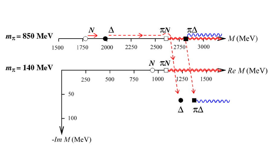
Figure 1: Movement of the $\Delta$ pole and the $\pi\Delta$ branch cut with change of pion mass in the LQCD results if variation w.r.t. $m_{\pi}$ would be smooth.

horizontal line labeled by $m_{\pi}=140$ MeV on the left, in Fig. 1. We have purposely aligned the two open squares corresponding to the $\pi N$ elastic threshold obtained with $m_{\pi}=850$ and $m_{\pi}=140$ MeV, respectively, to show more clearly how $\Delta$ pole moves as $m_{\pi}$ is varied. An experimental value of $\Gamma_{\Delta}=120$ MeV for the width of the $\Delta$ is assumed in Fig. 1 when $m_{\pi}=140$ MeV.

The pole character of the $\Delta$ in the $\pi N$ scattering amplitude would remain, as generally expected, unchanged after it moves into complex plane, if the singularity structure of the S matrix would vary smoothly with the pion mass. In the same

token, the branch point corresponding to the opening of $\pi\Delta$ would also move into complex plane and its squared root character should be retained as well. Accordingly, there should exist a branch cut in the complex plane starting from $m_{\pi}+M_{\Delta}$, which is complex when the value of $m_{\pi}$ goes down to 140 MeV, as indicated in Fig. 1.

3 Multiple poles structure of a resonance with several Riemann sheets

3.1 Number of Riemann sheets

The inclusion of the $\pi\Delta$ branch cut in the partial wave analysis in $P_{11}$ has led to the conclusion [1, 2, 8] that there are two almost degenerate poles corresponding to the Roper, one on the unphysical sheet directly reachable from the real axis and the other located just behind the $\pi\Delta$ cut. We demonstrate in the followings that such a two-pole structure could just be a direct mathematical consequence when there are two Riemann sheets to be considered.

The $\pi N$ T-matrix is a sum of background $T_{B}$ and resonances $T_{R}$ contributions, i.e., $T_{\pi N}=T_{B}+T_{R}$. The background $T_{B}$ contains branch points of elastic and all inelastic cuts. They appear additively and each of square root nature. For our purpose, we will first discuss the question of the number of Riemann sheets needed to make a function like $T_{B}$ single-valued in the presence of several branch points, all of square root nature.

It is known that a square root function $\sqrt{z}$ requires two Riemann sheets to make it single-valued. For a general case, we quote the following mathematical lemma [9], namely, $2^{n}$ Riemann sheets are required to make the function $f(z)=\sum_{i=1}^{n}\sqrt{z-z_{i}}$ single-valued. It is easy to see that the Riemann surface of a function of a more general form $f(z)=\sum_{i=1}^{n}g_{i}(z)\sqrt{z-z_{i}}$, where $g_{i}(z)$ are analytic functions, also contains $2^{n}$ sheets. Accordingly, the same conclusion should hold for $T_{B}$.

3.2 Multiple poles feature in the presence of branch cuts

We now turn to the cases where a pole is present in addition to branch cuts. Extension to several poles is straightforward. We’ll illustrate our mathematical argument with explicit examples, all have a pole at $z_{0}=r_{0}e^{i\theta_{0}},0\leq\theta_{0}\leq 2\pi$. For simplicity, we’ll assume that the background contribution behaves as $\sum_{i=1}^{n}\sqrt{z-z_{i}}$. In the followings, $g(z)$ denotes an analytic function and $a,b,z_{1},z_{2}$ are constants.

$$1.\,\,f_{1}(z) = \sqrt{z}+\frac{g(z)}{z-z_{0}}.$$

$$2.\,\,f_{2}(z) = \sqrt{z+z_{1}}+\frac{g(z)(\sqrt{z+z_{1}}\pm\sqrt{z_{0}+z_{1}})}{z-z_{0}}.$$

$$3.\,\,f_{3}(z) = \sqrt{z+z_{1}}+\sqrt{z+z_{2}}+\frac{g(z)}{z-z_{0}}.$$

$$4.\,\,f_{4}(z) = \sqrt{z+z_{1}}+\sqrt{z+z_{2}}+\frac{g(z)h(z)}{z-z_{0}},\,\,h(z)=a\sqrt{z+z_{1}}+b\sqrt{z_{0}+z_{1}}.$$

$$5.\,\,f_{5}(z) = \sqrt{z+z_{1}}+\sqrt{z+z_{2}}+\frac{g(z)(\sqrt{z+z_{1}}\pm\sqrt{z_{0}+z_{1}})(\sqrt{z+z_{2}}\pm\sqrt{z_{0}+z_{2}})}{z-z_{0}}.$$

The reason we consider only pole term of the form of $N(z)/(z-z_{0})$ is that we can always rewrite a function of the form $\tilde{N}(z)/D(Z)$, where $D(z)$ has a zero at $z_{0}$, as $N(z)/(z-z_{0})$ with $N(z)=[\tilde{N}(z)(z-z_{0})/D(z)]/(z-z_{0})$. With some simple mathematical analysis, it is not difficult

to reach the following conclusions, w.r.t. the numbers of Riemann sheets required to make the above functions single-valued and the multiplicity of the pole.
1. $f_{1}(z):$ Two Riemann sheets required. $r_{0}e^{i\theta_{0}}$ and $r_{0}e^{i(\theta_{0}+2\pi)}$, located in sheet I and II, respectively, are both poles of $f_{1}(z)$ with equal residue.
2. $f_{2}(z):$ Two Riemann sheets. Pole appears only in one Riemann sheet.
3. $f_{3}(z):$ Four Riemann sheets. Pole appears in every sheet with equal residue.
4. $f_{4}(z):$ Four Riemann sheets. Pole appears in every sheet but all with different residue. If $a=\pm b$, then pole appears only in two sheets.
5. $f_{5}(z):$ Four Riemann sheets. Pole appears only in one sheet.

Sheet	Position	Residue
I	1384 - 119$i$	19 - 68$i$
II	1382 - 138$i$	-6 - 105$i$
III	1513 - 54$i$	-15 - $i$
IV	1514 - 66$i$	-38 - 5$i$
I	1689 - 54$i$	-10 + 3$i$
II	1676 - 83$i$	-54 + 21$i$
III	1690 - 61$i$	-8 + 0$i$
IV	1683 - 83$i$	-39 + 12$i$

Table 1: The pole positions (MeV) and residues obtained in [2] by analyzing the VPI data of [1].

We are hence led to the conclusion that for a complex function with $n$ square root branch cuts, a pole could appear in all $2^{n}$ Riemann sheets or only some ($1,2,4,2^{n-1}$) of them, with equal or different residues. The multiplicity of the pole would reveal some information about the analytical structure of the numerator $N(z)=\tilde{N}(z)(z-z_{0})/D(z)$

4 Understanding the multiple-pole structure in $\pi N\,\,P_{11}$ channel

Table 1 gives the pole positions (MeV) and residues obtained in [2] by analyzing the VPI data of [1], where sheet I refers to the sheet most directly reached from real axis; sheet II is behind the $\pi\Delta$ branch cut, sheet III is behind the $\rho N$ branch cut, while sheet IV is behind both unstable-particle branch cuts. It is seen that pairs of poles, $(1384-119i,\,\,1382-138i),\,(1513-54i,\,\,1514-66i),\,(1513-54i,\,\,1514-66i),\,(1689-54i,\,\,1690-61i),\,(1676-83i,\,\,1683-83i)$ are all almost degenerate. In fact, the last two pairs are not very different from each other as well. The first pair $(1384-119i,\,\,1382-138i)$ was first noted by the SAID group [1] and recently received considerable attention from another perspective, e.g., see [8]. It will be very interesting to see whether those ”near degeneracies” are accidental or just manifestations of exact degeneracy, as discussed in the above, but masked by numerical indeterminacy. In any case, the exact number of degeneracy associated with any resonance as discussed here should be determined since it will give us some information about the numerator $N(z)$ which is related to the form factor of the resonance.

5 Summary

In summary, we present a simple heuristic argument to understand the existence of complex branch points in the $\pi N$ scattering amplitude. The reasoning is based on a hypothesis that the singularity structure of the $\pi N$ scattering amplitude is a smooth varying function of the pion mass. We then show that the two-pole structure found to correspond to the Roper resonance could just be a direct mathematical consequence of including additional Riemann surface in the study. In fact, our analysis indicates that it is always likely to find multiple poles, either two or four etc., to be associated with a resonance. It is useful to look for pole in all Riemann sheets to determine its multiplicity. It would provide us some information of the analytical structure of the numerator of the pole term, as the numerator of the pole term is related to resonance form factor.

References

- [1] R. A. Arndt, J. M. Ford, and L. D. Roper, Phys. Rev. D 32, 1085 (1985).
- [2] R. E. Cutkovsky, and S. Wang, Phys. Rev. D 42, 135 (1990).
- [3] R. E. Cutkovsky, C. P. Forsyth, R. E. Hendrick, and R. L. Kelly, Phys. Rev. D 20, 2839 (1990).
- [4] C. T. Hung, S. N. Yang, and T.-S. H. Lee, Phys. Rev. C 64, 034309 (2001); G. Y. Chen et al., Phys. Rev. C 76, 035206 (2007); L. Tiator et al., Phys. Rev. C 82, 055203 (2010).
- [5] S. Ceci et al., Phys. Rev. C 84, 015205 (2011).
- [6] S. N. Yang, Chin. J. Phys. 49, 1158 (2011); 51, 1107(E) (2013).
- [7] R. J. Eden, Proc. Roy. Soc. (London) A 210, 388 (1952); ibid. 217, 390 (1953).
- [8] N. Suzuki et al., Phys. Rev. Lett. 104, 042302 (2010).
- [9] C. L. Wang and W. Z. Yang, private communications.