On Certain Wronskians of Multiple Orthogonal Polynomials

On Certain Wronskians of Multiple Orthogonal
Polynomials

Lun ZHANG ^† and Galina FILIPUK ^‡

L. Zhang and G. Filipuk

^† School of Mathematical Sciences and Shanghai Key Laboratory for Contemporary
^† Applied Mathematics, Fudan University, Shanghai 200433, People’s Republic of China lunzhang@fudan.edu.cn http://homepage.fudan.edu.cn/lunzhang/

^‡ Faculty of Mathematics, Informatics and Mechanics, University of Warsaw,
^‡ Banacha 2, Warsaw, 02-097, Poland filipuk@mimuw.edu.pl http://www.mimuw.edu.pl/~filipuk/

Received August 01, 2014, in final form October 27, 2014; Published online November 04, 2014

We consider determinants of Wronskian type whose entries are multiple orthogonal polynomials associated with a path connecting two multi-indices. By assuming that the weight functions form an algebraic Chebyshev (AT) system, we show that the polynomials represented by the Wronskians keep a constant sign in some cases, while in some other cases oscillatory behavior appears, which generalizes classical results for orthogonal polynomials due to Karlin and Szegő. There are two applications of our results. The first application arises from the observation that the $m$-th moment of the average characteristic polynomials for multiple orthogonal polynomial ensembles can be expressed as a Wronskian of the type II multiple orthogonal polynomials. Hence, it is straightforward to obtain the distinct behavior of the moments for odd and even $m$ in a special multiple orthogonal ensemble – the AT ensemble. As the second application, we derive some Turán type inequalities for multiple Hermite and multiple Laguerre polynomials (of two kinds). Finally, we study numerically the geometric configuration of zeros for the Wronskians of these multiple orthogonal polynomials. We observe that the zeros have regular configurations in the complex plane, which might be of independent interest.

Wronskians; algebraic Chebyshev systems; multiple orthogonal polynomials; moments of the average characteristic polynomials; multiple orthogonal polynomial ensembles; Turán inequalities; zeros

05E35; 11C20; 12D10; 26D05; 41A50

1 Introduction and statement of the main results

1.1 Determinants whose entries are orthogonal polynomials

In a classical paper [39], Karlin and Szegő developed an interesting and general theory regarding the determinants whose entries are orthogonal polynomials [18, 31, 54]. They showed that the polynomials represented by certain determinants whose elements are orthogonal polynomials keep a constant sign in some cases, while in some other cases the polynomials are oscillatory. More precisely, let

$$Q_{n}(x)=k_{n}(-x)^{n}+\cdots,\qquad k_{n}>0,\qquad n\in\mathbb{N}=\{0,1,2,3,\ldots\},$$

be a sequence of orthogonal polynomials with respect to an arbitrary measure whose distribution function has an infinite number of increasing points. The Wronskian of these polynomials is then defined by

$$W(n,l;x):=W\left(Q_{n}(x),Q_{n+1}(x),\dots,Q_{n+l-1}(x)\right)$$

$$\phantom{W(n,l;x)}=\det\left(\begin{matrix}Q_{n}(x)&Q_{n+1}(x)&\cdots&Q_{n+l-1}(x)\\ Q_{n}^{\prime}(x)&Q_{n+1}^{\prime}(x)&\cdots&Q_{n+l-1}^{\prime}(x)\\ \vdots&\vdots&\vdots&\vdots\\ Q_{n}^{(l-1)}(x)&Q_{n+1}^{(l-1)}(x)&\cdots&Q_{n+l-1}^{(l-1)}(x)\\ \end{matrix}\right).$$

By [39, Theorems 1 and 2], it is known that, for $l$ even,

$$(-1)^{l/2}W(n,l;x)>0,\qquad x\in\mathbb{R},$$

i.e., the Wronskian keeps a constant sign for all real $x$; if $l$ is odd, then $W(n,l;x)$ has exactly $n$ simple real zeros and the zeros of $W(n,l;x)$ and $W(n+1,l;x)$ strictly interlace.

Another important class of determinants considered in [39] is the Hankel determinant

$$T(n,l;x):=T\left(Q_{n}(x),Q_{n+1}(x),\ldots,Q_{n+l-1}(x)\right)$$

$$\phantom{T(n,l;x)}=\det\left(\begin{matrix}Q_{n}(x)&Q_{n+1}(x)&\cdots&Q_{n+l-1}(x)\\ Q_{n+1}(x)&Q_{n+2}(x)&\cdots&Q_{n+l}(x)\\ \vdots&\vdots&\vdots&\vdots\\ Q_{n+l-1}(x)&Q_{n+l}(x)&\cdots&Q_{n+2l-2}(x)\\ \end{matrix}\right),$$

which is called the Turánian. Karlin and Szegő showed that, if $l$ is even, $T(n,l;x)$ has the sign $(-1)^{l/2}$ on the interval $I$ for the following three classical systems of orthogonal polynomials [54]:

• $Q_{n}(x)=P_{n}^{(\lambda)}(x)/P_{n}^{(\lambda)}(1)$, $\lambda>-1/2$ and $I=(-1,1)$, where $P_{n}^{(\lambda)}(x)$ are the ultraspherical polynomials,

• $Q_{n}(x)=L_{n}^{(\alpha)}(x)/L_{n}^{(\alpha)}(0)$, $\alpha>-1$ and $I=(0,+\infty)$, where $L_{n}^{(\alpha)}(x)$ are the Laguerre polynomials,

• $Q_{n}(x)=H_{n}(x)$ and $I=(-\infty,+\infty)$, where $H_{n}(x)$ are the Hermite polynomials.

The strategy of proofs is to represent the Hankel determinants in terms of the Wronskian of orthogonal polynomials of another type. Note that, if $l=2$, one has

$$T(n,2;x)=Q_{n+1}^{2}(x)-Q_{n}(x)Q_{n+2}(x)>0.$$

This inequality is called the Turán inequality, which was first proved for the Legendre polynomials $P_{n}(x)=P_{n}^{(1/2)}(x)$ [53, 55] and inspired the work of Karlin and Szegő. The analogous results for determinants involving orthogonal polynomials associated with discrete weights are also presented in [39].

Nowadays, determinants whose entries are orthogonal polynomials still attract much attention. For instance, the Wronskians of orthogonal polynomials also appear in random matrix theory; cf. [15, 47] and Section 3 below. The relationship between the Wronskian of orthogonal polynomials and the Hankel determinant of polynomials is clarified by Leclerc in [45], and further generalized by Durán [22]. In addition, it comes out that Turán inequality holds not only for a large class of orthogonal polynomials including the most classical orthogonal polynomials (cf. [10, 17, 23, 24, 29, 30, 41, 51, 52]), but also for many special functions and their $q$-analogues with important applications; we refer to [1, 6, 7, 8, 9, 20, 37, 44, 46, 49, 50] and the references therein for the development of that aspect. Other studies of the Wronkians of orthogonal polynomials can be found in [36, 38, 59].

In this paper, we are concerned with the Wronskians of multiple orthogonal polynomials. Since multiple orthogonal polynomials are generalizations of orthogonal polynomials, our results extend the aforementioned results for orthogonal polynomials. In what follows, we first give a brief introduction to multiple orthogonal polynomials and fix the notations used throughout this paper, and next state the main results and outline the rest of the paper.

1.2 Multiple orthogonal polynomials and algebraic Chebyshev (AT) systems

Multiple orthogonal polynomials are polynomials of one variable which are defined by orthogonality relations with respect to $r$ different weights $w_{1},w_{2},\ldots,w_{r}$, where $r\geq 1$ is a positive integer. They originated from Hermite–Padé approximation in the context of irrationality and transcendence proofs in number theory, and they were further developed in approximation theory; cf. [2, 4, 16, 32, 48] and surveys [3, 56, 57].

Let $\vec{n}=(n_{1},n_{2},\ldots,n_{r})\in\mathbb{N}^{r}$ be a multi-index of size $|\vec{n}|=n_{1}+n_{2}+\dots+n_{r}$ and suppose $w_{1},w_{2},\ldots,w_{r}$ are $r$ weights with supports on the real axis. There are two types of multiple orthogonal polynomials. The type I multiple orthogonal polynomials are given by the vector $(A_{\vec{n},1},\ldots,A_{\vec{n},r})$, where $A_{\vec{n},j}$ is a polynomial of degree $\leq n_{j}-1$, such that the linear form

$$Q_{\vec{n}}(x)=\sum\limits_{j=1}^{r}A_{\vec{n},j}(x)w_{j}(x)$$ (1.1)

satisfies

$$\int Q_{\vec{n}}(x)x^{k}\,dx=0,\qquad k=0,1,\ldots,|\vec{n}|-2.$$ (1.2)

By setting the normalization condition

$$\int Q_{\vec{n}}(x)x^{|\vec{n}|-1}\,dx=1,$$ (1.3)

the equations (1.2), (1.3) form a linear system of $|\vec{n}|$ equations for the unknown coefficients of $A_{\vec{n},1},\ldots,A_{\vec{n},r}$. The multi-index $\vec{n}$ is called normal if this linear system has a unique solution, i.e., the polynomials of vector $(A_{\vec{n},1},\ldots,A_{\vec{n},r})$ exist uniquely. The type II multiple orthogonal polynomial is the monic polynomial $P_{\vec{n}}(x)=x^{|\vec{n}|}+\cdots$ of degree $|\vec{n}|$ satisfying the conditions

$$\int P_{\vec{n}}(x)x^{k}w_{1}(x)\,dx=0,\qquad k=0,1,\ldots,n_{1}-1,$$

$$\cdots\cdots\cdots\cdots\cdots\cdots\cdots\cdots\cdots\cdots\cdots\cdots\cdots\cdots\cdots\cdots$$ (1.4)

$$\int P_{\vec{n}}(x)x^{k}\,w_{r}(x)\,dx=0,\qquad k=0,1,\ldots,n_{r}-1.$$

The polynomials $P_{\vec{n}}$ exist and are unique whenever $\vec{n}$ is a normal index.

Under certain additional conditions on $r$ weights, we can ensure the uniqueness and existence of multiple orthogonal polynomials. One of such conditions is that the weight functions form a so-called algebraic Chebyshev (AT) system; cf. [35, Section 23.1.2].

A Chebyshev system $\{\varphi_{1},\ldots,\varphi_{n}\}$ on $[a,b]$ is a system of $n$ linearly independent functions such that every linear combination $\sum\limits_{k=1}^{n}a_{k}\varphi_{k}$ has at most $n-1$ zeros on $[a,b]$. Equivalently, this means that

$$\det\begin{pmatrix}\varphi_{1}(x_{1})&\varphi_{1}(x_{2})&\cdots&\varphi_{1}(x_{n})\\ \varphi_{2}(x_{1})&\varphi_{2}(x_{2})&\cdots&\varphi_{2}(x_{n})\\ \vdots&\vdots&\cdots&\vdots\\ \varphi_{n}(x_{1})&\varphi_{n}(x_{2})&\cdots&\varphi_{n}(x_{n})\end{pmatrix}\neq 0,$$

for every choice of $n$ different points $x_{1},\ldots,x_{n}\in[a,b]$. To see this, suppose $x_{1},\ldots,x_{n}$ are such that the determinant is zero, then there is a linear combination of the rows $\sum\limits_{k=1}^{n}b_{k}\varphi_{k}$ that gives a zero row. We then obtain a linear combination of functions $\varphi_{k}$ admitting $n$ zeros at $x_{1},\ldots,x_{n}$, which is a contradiction.

A system of $r$ weights $(w_{1},\ldots,w_{r})$ is an AT system for the multi-index $\vec{n}$ if each $w_{j}$ is defined on a fixed interval $[a,b]\subseteq\mathbb{R}$ such that

$$\big{\{}w_{1},xw_{1},\ldots,x^{n_{1}-1}w_{1},w_{2},xw_{2},\ldots,x^{n_{2}-1}w_{2},\ldots,w_{r},xw_{r},\ldots,x^{n_{r}-1}w_{r}\big{\}}$$

is a Chebyshev system on $[a,b]$. If $\vec{n}$ is a multi-index such that the weights $(w_{1},\ldots,w_{r})$ form an AT system for every index $\vec{m}$ satisfying $\vec{m}\leq\vec{n}$ (in the componentwise sense, that is, $m_{j}\leq n_{j}$, $j=1,\ldots,r$), by [35, Theorem 23.2]. We have that $\vec{n}$ is a normal index, which implies the existence and uniqueness of the polynomials $P_{\vec{n}}$. In particular, the weights for many classical multiple orthogonal polynomials (including multiple Hermite polynomials, multiple Laguerre polynomials, Jacobi–Piñeiro polynomials) belong to the AT systems.

For more information about multiple orthogonal polynomials, we refer to Aptekarev et al. [3, 5], Coussement and Van Assche [58], Nikishin and Sorokin [48, Chapter 4, § 3], Ismail [35, Chapter 23] and Filipuk, Van Assche and Zhang [26].

1.3 Statement of the main results

To state our main results, we need to define the Wronskian of multiple orthogonal polynomials. Let us consider a sequence of multi-indices $(\vec{n}_{0},\vec{n}_{1},\ldots,\vec{n}_{l-1})$, $l\in\mathbb{Z}^{+}=\{1,2,3,\ldots\}$, such that

• $\vec{n}_{0}=\vec{n}$ for a given initial multi-index $\vec{n}$,

• $|\vec{n}_{j}|=|\vec{n}|+j$ for $j=1,\ldots,l-1$,

• $\vec{n}_{0}\leq\vec{n}_{1}\leq\dots\leq\vec{n}_{l-2}\leq\vec{n}_{l-1}$ (componentwise).

Therefore, $(\vec{n}_{0},\vec{n}_{1},\ldots,\vec{n}_{l-1})$ defines a path connecting $\vec{n}$ to $\vec{n}_{l-1}$, where in each step the multi-index $\vec{n}_{k}$ is increased by one in exactly one direction.

For every such kind of a fixed path, we define the associated Wronskian of multiple orthogonal polynomials by

$$W(\vec{n},l;x):=W\left(P_{\vec{n}_{0}}(x),P_{\vec{n}_{1}}(x),\ldots,P_{\vec{n}_{l-1}}(x)\right)$$

$$\phantom{W(\vec{n},l;x)}=\det\left(\begin{matrix}P_{\vec{n}_{0}}(x)&P_{\vec{n}_{1}}(x)&\cdots&P_{\vec{n}_{l-1}}(x)\\ P_{\vec{n}_{0}}^{\prime}(x)&P_{\vec{n}_{1}}^{\prime}(x)&\cdots&P_{\vec{n}_{l-1}}^{\prime}(x)\\ \vdots&\vdots&\vdots&\vdots\\ P_{\vec{n}_{0}}^{(l-1)}(x)&P_{\vec{n}_{1}}^{(l-1)}(x)&\cdots&P_{\vec{n}_{l-1}}^{(l-1)}(x)\end{matrix}\right),$$ (1.5)

where $P_{\vec{n}}$ is the type II multiple orthogonal polynomial given in (1.4). Clearly, $W(\vec{n},l;x)$ is a polynomial in $x$ depending on the parameters $\vec{n}$, $l$ and the path starting from $\vec{n}$. We shall also use the notation $W(\vec{a},\vec{b},\ldots,\vec{e};x)$ to emphasize the dependence on a specific path consisting of the multi-indices $(\vec{a},\vec{b},\ldots,\vec{e})$ if necessary.

Our main results are stated as follows.

Theorem 1.1.

Suppose that the weights $(w_{1},w_{2},\ldots,w_{r})$ form an AT system on $[a,b]$ for all the multi-indices $\vec{n}\in\mathbb{N}^{r}$, then we have

$$W(\vec{n},l;x)>0,\qquad x\in\mathbb{R},$$ (1.6)

if $l$ is even, where $W(\vec{n},l;x)$ is defined in (1.5).

Note that our assumption on the weights ensures the existence of multiple orthogonal polynomials (see the discussion at the end of the previous section), thus the Wronskian is well-defined. If $l$ is odd, then we have the following result.

Theorem 1.2.

Let $w_{1},w_{2},\ldots,w_{r}$ be $r$ weights as in Theorem 1.1 and let $l$ be odd. For each fixed multi-index $\vec{n}$ the polynomials $W(\vec{n},l;x)$ have exactly $|\vec{n}|$ simple zeros on the real axis. Furthermore, given two paths consisting of $l$ multi-indices such that the last $l-1$ multi-indices of one path starting from $\vec{n}$ coincide with the first $l-1$ multi-indices of the other path ending at $\vec{m}$ $($which also means $|\vec{m}|=|\vec{n}|+l$ and $\vec{n}\leq\vec{m})$, then the real zeros of two associated Wronskians strictly interlace.

In case $l=1$, this theorem states that the type II multiple orthogonal polynomial $P_{\vec{n}}$ whose weights form an AT system has $|\vec{n}|$ zeros and the zeros of $P_{\vec{n}}$ and $P_{\vec{n}+\vec{e}_{k}}$ ($k=1,\ldots,r$) interlace, where $\vec{e}_{k}=(0,\ldots,0,1,0,\ldots,0)$ denotes the $k$-th standard unit vector with 1 on the $k$-th entry. These facts are already known; cf. [35, Theorem 23.2] and [33]. Moreover, if $r=1$, the type II multiple orthogonal polynomials reduce to the usual orthogonal polynomials, hence, Theorems 1.1 and 1.2 generalize classical results of Karlin and Szegő mentioned at the beginning.

Finally, one can also consider the Wronskians involving type I multiple orthogonal polynomials by replacing $P_{\vec{n}}$ in (1.5) by $Q_{\vec{n}}$ defined in (1.1). In this case, the Wronskians are not polynomials in general.

Theorem 1.3.

Let $w_{1},w_{2},\ldots,w_{r}$ be $r$ sufficiently many times differentiable weights as in Theorem 1.1 and assume that $l$ is even. For each path starting from the multi-index $\vec{n}$, we have that the function $W(Q_{\vec{n}}(x),Q_{\vec{n}_{1}}(x),\ldots,Q_{\vec{n}_{l-1}}(x))$ given in (1.5) keeps a constant sign on $(a,b)$, if the Wronskian is well defined.

1.4 Outline of the paper

The rest of this paper is organized as follows. In Section 2, we prove Theorems 1.1–1.3. We next give two applications of our main results. In Section 3, we show that the $m$-th moment of the average characteristic polynomials for multiple orthogonal polynomial ensembles can be expressed as a Wronskian of the type II multiple orthogonal polynomials. It is then straightforward to obtain the distinct behavior of the moments for odd and even $m$ in a special multiple orthogonal ensemble – the AT ensemble. In Section 4 we derive the inequalities of Turán type for some classical multiple orthogonal polynomials, namely, for multiple Hermite polynomials and multiple Laguerre polynomials. We conclude this paper with numerical study of the zero configurations of the Wronskians for multiple Hermite polynomials and multiple Laguerre polynomials in Section 5. It comes out that the zeros have fascinating and regular configurations in the complex plane, which might be of independent interest.

2 Proofs of Theorems 1.1–1.3

We shall prove our main theorems by extending the arguments in [39]. Roughly speaking, the proofs of Theorems 1.1 and 1.3 use the properties of an AT system, while for the proof of Theorem 1.2 one needs Theorem 1.1 and Sylvester’s theorem concerning the relation between the determinants of a square matrix and its minors.

2.1 Proof of Theorem 1.1

We first show that the Wronskian (1.6) keeps a constant sign on the real axis for $l$ even. If this is not true, we may find a real number $x_{0}$ such that $W(\vec{n},l;x_{0})=0$. This in turn implies the existence of the constants $\lambda_{0},\lambda_{1},\ldots,\lambda_{l-1}$ depending on the path such that the function

$$f(x):=\sum\limits_{i=0}^{l-1}\lambda_{i}P_{\vec{n}_{i}}(x)$$ (2.1)

satisfies

$$f^{(k)}(x_{0})=0,\qquad k=0,1,\ldots,l-1.$$

Thus, $x_{0}$ is a zero of $f(x)$ of multiplicity at least $l$.

We further claim that $f$ has at least $|\vec{n}|$ zeros on $(a,b)$ where $f$ changes sign. Such zeros are also called nodal zeros. To see this, we first observe from (1.4) and (2.1) that the equality

$$\int f(x)\sum\limits_{i=1}^{r}q_{i}(x)w_{i}(x)\,dx=0$$ (2.2)

holds for any polynomials $q_{i}(x)$ of degree less than or equal to $n_{i}-1$, where we also make use of the fact that $\vec{n}\leq\vec{n}_{1}\leq\dots\leq\vec{n}_{l-2}\leq\vec{n}_{l-1}$. In order to obtain a contradiction, suppose that $f$ has at most $k\leq|\vec{n}|-1$ nodal zeros on $(a,b)$, say, $x_{1},x_{2},\ldots,x_{k}$, then

$$f(x)=\prod\limits_{i=1}^{k}(x-x_{i})Q(x),$$ (2.3)

where $Q$ does not change the sign on the the interval $(a,b)$. Since $k\leq|\vec{n}|-1$, it is always possible to construct a multi-index $\vec{m}=(m_{1},m_{2},\ldots,m_{r})\in\mathbb{N}^{r}$ such that $\vec{m}\leq\vec{n}$, and $|\vec{m}|=k+1\leq|\vec{n}|$ for any given initial multi-index $\vec{n}$. Then there exist polynomials $\widetilde{q}_{i}$, $1\leq i\leq r$, with degrees less than or equal to $m_{i}-1$ satisfying

$$\sum\limits_{i=1}^{r}\widetilde{q}_{i}(x)w_{i}(x)=\begin{cases}0,&\text{if}\quad x=x_{1},x_{2},\ldots,x_{k},\\ 1,&\text{if}\quad x=x_{k+1},\end{cases}$$

where $x_{1},x_{2},\ldots,x_{k}$ are the nodal zeros as in (2.3) and $x_{k+1}$ is an arbitrary point on $(a,b)$ but different from those $k$ nodal zeros. Indeed, this is equivalent to solving a linear system of $|\vec{m}|=k+1$ equations for the unknown coefficients of $\widetilde{q}_{i}$. This system is uniquely solvable if the matrix

$$\left(\begin{matrix}w_{1}(x_{1})&\cdots&x_{1}^{m_{1}-1}w_{1}(x_{1})\\ w_{1}(x_{2})&\cdots&x_{2}^{m_{1}-1}w_{1}(x_{2})\\ \vdots&\vdots&\vdots\\ w_{1}(x_{k+1})&\cdots&x_{k+1}^{m_{1}-1}w_{1}(x_{k+1})\end{matrix}\cdots\cdots\begin{matrix}w_{r}(x_{1})&\cdots&x_{1}^{m_{r}-1}w_{r}(x_{1})\\ w_{r}(x_{2})&\cdots&x_{2}^{m_{r}-1}w_{r}(x_{2})\\ \vdots&\vdots&\vdots\\ w_{r}(x_{k+1})&\cdots&x_{k+1}^{m_{r}-1}w_{r}(x_{k+1})\end{matrix}\right)$$

is not singular, which is immediate on account of the fact that our weights $(w_{1},w_{2},\ldots,w_{r})$ form an AT system on $[a,b]$ for all the multi-indices. The Chebyshev property further indicates that the function $\prod\limits_{i=1}^{k}(x-x_{i})(\sum\limits_{i=1}^{r}\widetilde{q}_{i}(x)w_{i}(x))$ does not change the sign on $(a,b)$ (cf. [40]). This, together with (2.3), implies that

$$\int f(x)\sum\limits_{i=1}^{r}\widetilde{q}_{i}(x)w_{i}(x)\,dx\neq 0,$$

which is a contradiction with (2.2). Thus, we have proved $f$ has at least $|\vec{n}|$ nodal zeros on $(a,b)$.

Note that our definition of $f$ in (2.1) shows that $f$ is a polynomial of degree less than or equal to $|\vec{n}|+l-1$. If $x_{0}$ is different from all these nodal zeros, then $f$ will have at least $|\vec{n}|+l$ zeros, which is a contradiction. On the other hand, if $x_{0}$ coincides with one of the nodal zeros, multiplicity of $x_{0}$ must be at least $l+1$ (since the zero of even multiplicity $l$ cannot be nodal), hence, the number of total zeros is at least $|\vec{n}|-1+l+1=|\vec{n}|+l$, again a contradiction. In summary, we have proved that $W(\vec{n},l;x)$ keeps a constant sign on the real axis if $l$ is even.

Finally, the inequality (1.6) follows from the observation that the leading term of the $W(\vec{n},l;x)$ is $x^{l|\vec{n}|}$, up to a positive constant. This can be seen by first multiplying the rows of (1.5) by $1,x,\ldots,x^{l-1}$ and the columns by $x^{-|\vec{n}|},x^{-|\vec{n}|-1},\ldots,x^{-|\vec{n}|-l+1}$, respectively, and then letting $x\to\infty$.

2.2 Proof of Theorem 1.2

The proof of this theorem is similar to that for the case of orthogonal polynomials in [39]. We start with a special form of Sylvester’s identity which states that for any square matrix $A$ of size $n$ and $n\geq m_{1}\geq m_{2}\geq 1$ and $n\geq n_{1}>n_{2}\geq 1$, the following identity (cf. [28]) holds:

$$\det A\cdot\det A[m_{1},m_{2};n_{1},n_{2}]=\det\begin{pmatrix}\det A[m_{1};n_{1}]&\det A[m_{1};n_{2}]\\ \det A[m_{2};n_{1}]&\det A[m_{2};n_{2}]\end{pmatrix},$$ (2.4)

where $A[m_{1},m_{2};n_{1},n_{2}]$ denotes the submatrix obtained from $A$ by deleting rows $m_{1}$, $m_{2}$ and columns $n_{1}$, $n_{2}$, and a similar definition holds for $A[m_{i};n_{j}]$, $i,j=1,2$.

Given any path, say, $(\vec{n}_{0},\vec{n}_{1},\ldots,\vec{n}_{l-1})$, we can find another path $(\vec{n}_{1},\vec{n}_{2},\ldots,\vec{n}_{l})$ whose first $l-1$ multi-indices coincide with the last $l-1$ multi-indices of the original path. Applying (2.4) to $\det A=W(\vec{n}_{0},\vec{n}_{1},\ldots,\vec{n}_{l-1},\vec{n}_{l};x)$ with $m_{1}=l+1$, $m_{2}=l$ and $n_{1}=l+1$, $n_{2}=1$, we have

$$W(\vec{n}_{0},\ldots,\vec{n}_{l};x)\cdot W(\vec{n}_{1},\ldots,\vec{n}_{l-1};x)=\det\begin{pmatrix}W(\vec{n}_{0},\ldots,\vec{n}_{l-1};x)&W(\vec{n}_{1},\ldots,\vec{n}_{l};x)\\ W^{\prime}(\vec{n}_{0},\ldots,\vec{n}_{l-1};x)&W^{\prime}(\vec{n}_{1},\ldots,\vec{n}_{l};x)\end{pmatrix},$$

where the derivative ^′ is with respect to $x$. Recall that $l$ is odd, hence, Theorem 1.1 gives us

$$W(\vec{n}_{0},\ldots,\vec{n}_{l-1};x)W^{\prime}(\vec{n}_{1},\ldots,\vec{n}_{l};x)-W^{\prime}(\vec{n}_{0},\ldots,\vec{n}_{l-1};x)W(\vec{n}_{1},\ldots,\vec{n}_{l};x)>0,$$

for all $x\in\mathbb{R}$. This inequality shows that all zeros of $W(\vec{n}_{0},\ldots,\vec{n}_{l-1};x)$ must be simple. Moreover, we have

$$W(\vec{n}_{0},\ldots,\vec{n}_{l-1};x)W^{\prime}(\vec{n}_{1},\ldots,\vec{n}_{l};x)>0,\qquad\textrm{if}\qquad W(\vec{n}_{1},\ldots,\vec{n}_{l};x)=0,$$ (2.5)

and

$$W^{\prime}(\vec{n}_{0},\ldots,\vec{n}_{l-1};y)W(\vec{n}_{1},\ldots,\vec{n}_{l};y)<0,\qquad\textrm{if}\qquad W(\vec{n}_{0},\ldots,\vec{n}_{l-1};y)=0.$$ (2.6)

If $x_{0}$ and $\widetilde{x}_{0}$ are two consecutive zeros of $W(\vec{n}_{1},\ldots,\vec{n}_{l};x)$, then

$$W^{\prime}(\vec{n}_{1},\ldots,\vec{n}_{l};x_{0})W^{\prime}(\vec{n}_{1},\ldots,\vec{n}_{l};\widetilde{x}_{0})<0.$$

This, together with (2.5), implies that

$$W(\vec{n}_{0},\ldots,\vec{n}_{l-1};x_{0})W(\vec{n}_{0},\ldots,\vec{n}_{l-1};\widetilde{x}_{0})<0.$$

Hence, there must be a zero of $W(\vec{n}_{0},\ldots,\vec{n}_{l-1};x)$ between $(x_{0},\widetilde{x}_{0})$. By (2.6) and the same argument, we conclude that there exists at least one zero of $W(\vec{n}_{1},\ldots,\vec{n}_{l};x)$ between any two consecutive zeros of $W(\vec{n}_{0},\ldots,\vec{n}_{l-1};x)$. This completes the proof of the simplicity and the interlacing property of real zeros stated in Theorem 1.2.

Finally, it remains to calculate the number of real zeros of the Wronskian. This can be achieved by induction argument on $|\vec{n}|$. If $|\vec{n}|=0$ (i.e., $\vec{n}=\vec{0}$), then $W(\vec{0},l;x)>0$, since the Wronskian matrix reduces to the upper diagonal matrix with positive diagonal entries. Hence, there is no real zero in this case. If $|\vec{n}|=1$, we have $W(\vec{n},l;x)\sim x^{|\vec{n}|l}=x^{l}$ as $x\to\pm\infty$ and $l$ is odd, thus, $W(\vec{n},l;x)$ has at least one real zero. If it has more than one real zero, by interlacing property this will lead to the existence of a real zero for certain Wronskian associated with a path starting from $\vec{0}$, hence, a contradiction. Suppose now that $W(\vec{n},l;x)$ has exactly $k>0$ simple real zeros if $|\vec{n}|=k$. When $|\vec{n}|=k+1$, for any path starting from $\vec{n}$, we can find another path starting from $\vec{m}$ such that $|\vec{m}|=k$ and the zeros of $W(\vec{n},l;x)$ and $W(\vec{m},l;x)$ interlace. Then, $W(\vec{n},l;x)$ will have at least $k-1$ simple zeros. If $x_{k}$ is the largest zero of $W(\vec{m},l;x)$, then $W^{\prime}(\vec{m},l;x_{k})>0$ since $W(\vec{m},l;x)$ is positive for $x$ large. From (2.6), we have that $W(\vec{n},l;x_{k})<0$, hence there will be at least one zero of $W(\vec{n},l;x)$ on the right hand side of $x_{k}$. There would be only one such zero, again by interlacing property. Similar argument implies that there will be exactly one zero on the left of the smallest real zero of $W(\vec{m},l;x)$. Thus, $W(\vec{n},l;x)$ will have exactly $k+1=|\vec{n}|$ real simple zeros.

2.3 Proof of Theorem 1.3

The proof is similar to that of Theorem 1.1. Suppose that there exists a point $x_{0}\in(a,b)$ such that $W(Q_{\vec{n}}(x_{0}),Q_{\vec{n}_{1}}(x_{0}),\ldots,Q_{\vec{n}_{l-1}}(x_{0}))=0$. Then we can find constants $\lambda_{i}$, $i=0,1,\ldots,l-1$, such that the function

$$f(x):=\sum\limits_{i=0}^{r-1}\lambda_{i}Q_{\vec{n}_{i}}(x),\qquad\vec{n}_{0}=\vec{n},$$

has a zero at $x_{0}$ of multiplicity at least $l$. Since

$$\int f(x)p(x)\,dx=0$$

for any polynomial $p$ of degree less than or equal to $|\vec{n}|-2$, we have that $f$ has at least $|\vec{n}|-1$ nodal zeros. Thus, as in the proof of Theorem 1.1, we conclude that $f$ will have at least $|\vec{n}|+l-1$ zeros. This is a contradiction to the fact that $f$ is a linear combination of the Chebyshev system for the multi-index $\vec{n}_{l-1}$, which has at most $|\vec{n}_{l-1}|-1=|\vec{n}|+l-2$ zeros on $[a,b]$.

3 Moments of the average characteristic polynomials
for multiple orthogonal polynomial ensembles

In this section, we shall apply our results to the moments of the average characteristic polynomials for multiple orthogonal polynomial ensembles.

It is well-known that, besides the interest from the approximation theory, multiple orthogonal polynomials have also arisen recently in a natural way in certain models of mathematical physics, including random matrix theory, non-intersecting paths, etc; cf. [42, 43] and the references therein. Indeed, let us consider $|\vec{n}|=\sum\limits_{i=1}^{r}n_{i}=n$ random points on the real line whose joint probability density function (p.d.f.) can be written as a product of two determinants:

$$\frac{1}{Z_{n}}\det\left(f_{i}(x_{j})\right)_{i,j=1}^{n}\det\left(g_{i}(x_{j})\right)_{i,j=1}^{n},$$ (3.1)

where $Z_{n}$ is the normalizing constant to make the total probability on $\mathbb{R}^{n}$ equal to one, and the two sequences of functions $f_{i}$, $g_{i}$ are given by

$$f_{i}(x)=x^{i-1},\qquad i=1,\ldots,n,$$

and

$$g_{i}(x)=x^{i-1}w_{1}(x),\qquad i=1,\ldots,n_{1},$$

$$g_{n_{1}+i}(x)=x^{i-1}w_{2}(x),\qquad i=1,\ldots,n_{2},$$

$$\cdots\cdots\cdots\cdots\cdots\cdots\cdots\cdots\cdots\cdots\cdots\cdots\cdots\cdots\cdots\cdots$$

$$g_{n_{1}+\dots+n_{r-1}+i}(x)=x^{i-1}w_{r}(x),\qquad i=1,\ldots,n_{r}.$$

We call this stochastic model a multiple orthogonal polynomial ensemble, since one has

$$P_{\vec{n}}(z)=\mathbb{E}\left[\prod\limits_{k=1}^{n}(z-x_{k})\right],\qquad z\in\mathbb{C},$$ (3.2)

where the expectation $\mathbb{E}$ is taken with respect to the p.d.f. (3.1).

The formula (3.2) tells us that the type II multiple orthogonal polynomial $P_{\vec{n}}(z)$ can be viewed as the average of the random polynomials $\prod\limits_{k=1}^{n}(z-x_{k})$ whose roots are distributed according to (3.1). As a consequence, $P_{\vec{n}}$ is also called the average characteristic polynomial if the distribution (3.1) can be interpreted as the particle distribution of certain stochastic models. In particular, we mention that one example falling into this category is from the random matrix model with external source [13, 14, 60], which was first observed in [11].

The result (3.2) is further extended by Delvaux in [21] to arbitrary products and ratios of characteristic polynomials, which are defined by

$$\mathbb{E}\left[\frac{\prod\limits_{j=1}^{m}\prod\limits_{k=1}^{n}(z_{j}-x_{k})}{\prod\limits_{j=1}^{l}\prod\limits_{k=1}^{n}(y_{j}-x_{k})}\right],\qquad l,m,n\in\mathbb{N},$$

where $z_{1},\ldots,z_{m}\in\mathbb{C}$, $y_{1},\ldots,y_{l}\in\mathbb{C}\setminus\mathbb{R}$, and all the numbers in the set $(z_{1},\ldots,z_{m},y_{1},\ldots,y_{l})$ are pairwise different. It turns out that the products/ratios of the average characteristic polynomials for multiple orthogonal polynomial ensembles can be expressed as the determinants whose entries involve the blocks of the Riemann–Hilbert matrix characterizing multiple orthogonal polynomials and a matrix-valued version of the Christoffel–Darboux kernel. Particularly, in case $l=0$, it follows from [21, Theorem 1.8] that

$$\mathbb{E}\left[\prod\limits_{j=1}^{m}\prod\limits_{k=1}^{n}\!(z_{j}-x_{k})\right]=\frac{1}{\prod\limits_{1\leq i<j\leq m}(z_{j}-z_{i})}\det\!\left(\begin{matrix}P_{\vec{n}_{0}}(z_{1})&P_{\vec{n}_{1}}(z_{1})&\cdots&P_{\vec{n}_{m-1}}(z_{1})\\ P_{\vec{n}_{0}}(z_{2})&P_{\vec{n}_{1}}(z_{2})&\cdots&P_{\vec{n}_{m-1}}(z_{2})\\ \vdots&\vdots&\vdots&\vdots\\ P_{\vec{n}_{0}}(z_{m})&P_{\vec{n}_{1}}(z_{m})&\cdots&P_{\vec{n}_{m-1}}(z_{m})\end{matrix}\right)\!,\!\!\!$$ (3.3)

where $\vec{n}_{0}=\vec{n}$, $\vec{n}_{k}\geq\vec{n}_{k-1}$ componentwise and $|\vec{n}_{k}-\vec{n}_{k-1}|=1$ for $k=1,\ldots,m$, which is actually an arbitrary path connecting $\vec{n}_{0}$ to $\vec{n}_{m-1}$; see the definition at the beginning of Section 1.3.

Now, let all $z_{j}$ in (3.3) tend to $z$, an algebraic manipulation (cf. [34, Theorem 1.2.4]) shows that the moments of the average characteristic polynomials for multiple orthogonal polynomial ensembles can be expressed as the Wronskians of type II multiple orthogonal polynomials:

$$\mathbb{E}\left[\prod\limits_{k=1}^{n}(z-x_{k})^{m}\right]=\frac{1}{\prod\limits_{i=0}^{m-1}i!}W\left(P_{\vec{n}_{0}}(z),P_{\vec{n}_{1}}(z),\ldots,P_{\vec{n}_{m-1}}(z)\right),$$ (3.4)

where $W$ is defined in (1.5). Note that when $g_{i}(x)=x^{i-1}w(x)$ in (3.1) (i.e., in the case of orthogonal polynomial ensembles), the formula above was first shown by Brézin and Hikami [15]; see also [47].

Combining (3.4) and Theorems 1.1–1.2, we obtain

Corollary 3.1.

Assume that the weights $(w_{1},w_{2},\ldots,w_{r})$ in (3.1) form an AT system on $[a,b]$ for all the multi-indices in $\mathbb{N}^{r}$ $($i.e., an AT ensemble in the sense of [42]). Then we have that the moments of the average characteristic polynomials with respect to (3.1)

$$\mathbb{E}\left[\prod\limits_{k=1}^{n}(z-x_{k})^{m}\right]$$

are strictly positive on the real axis if $m$ is even; while for odd $m$, the moments admit oscillatory behavior as stated in Theorem 1.2.

4 Some inequalities for multiple orthogonal polynomials

In this section, we shall use our results to derive the inequalities of Turán type for some classical multiple orthogonal polynomials, namely, for multiple Hermite polynomials and multiple Laguerre polynomials. It is known that the weights for these polynomials form an AT system for any multi-index $\vec{n}\in\mathbb{N}^{r}$.

4.1 Turán inequalities for multiple Hermite polynomials

Multiple Hermite polynomials are defined by

$$\int_{-\infty}^{\infty}x^{k}H_{\vec{n}}(x)e^{-x^{2}+c_{j}x}\,dx=0,\qquad k=0,1,\ldots,n_{j}-1,$$

for $j=1,\ldots,r$, where $c_{i}\neq c_{j}$ if $i\neq j$; cf. [12], [35, § 23.5] and [58, § 3.4]. An explicit formula for multiple Hermite polynomials is

$$H_{\vec{n}}=\frac{(-1)^{|\vec{n}|}}{2^{|\vec{n}|}}\sum\limits_{k_{1}=0}^{n_{1}}\cdots\sum\limits_{k_{r}=0}^{n_{r}}\binom{n_{1}}{k_{1}}\cdots\binom{n_{r}}{k_{r}}\prod\limits_{j=1}^{r}c_{j}^{n_{j}-k_{j}}(-1)^{|\vec{k}|}H_{|\vec{k}|}(x),$$

where $\vec{k}=(k_{1},\ldots,k_{r})$ and $H_{|\vec{k}|}$ is the usual Hermite polynomial of degree $|\vec{k}|$ with the leading coefficient $2^{|\vec{k}|}$. The following statement holds for multiple Hermite polynomials.

Theorem 4.1.

The multiple Hermite polynomials satisfy the following inequalities:

$$H_{\vec{n}+\vec{e}_{j}}(x)H_{\vec{n}+\vec{e}_{k}}(x)-H_{\vec{n}}(x)H_{\vec{n}+\vec{e}_{j}+\vec{e}_{k}}(x)>0,\qquad x\in\mathbb{R},$$ (4.1)

for $j,k=1,\ldots,r$, where $\vec{e}_{i}=(0,\ldots,0,1,0,\ldots,0)$ denotes the $i$-th standard unit vector with $1$ on the $i$-th entry. In particular, by taking $j=k$, we have

$$H_{\vec{n}+\vec{e}_{j}}^{2}(x)-H_{\vec{n}}(x)H_{\vec{n}+2\vec{e}_{j}}(x)>0,\qquad x\in\mathbb{R}.$$ (4.2)

Remark 4.2.

It is readily seen that the formula (4.2) extends the Turán inequality for the Hermite polynomials [39].

Proof.

From Theorem 1.1 with $l=2$, it follows that

$$\det\begin{pmatrix}H_{\vec{n}}(x)&H_{\vec{n}+\vec{e}_{j}}(x)\\ H_{\vec{n}}^{\prime}(x)&H_{\vec{n}+\vec{e}_{j}}^{\prime}(x)\end{pmatrix}>0,\qquad j=1,\ldots,r,$$ (4.3)

for any $x\in\mathbb{R}$. Note that $H_{\vec{n}}$ satisfies the following raising operations (cf. [35, § 23.8.2])

$$\frac{d}{dx}\big{(}e^{-x^{2}+c_{k}x}H_{\vec{n}}(x)\big{)}=-2e^{-x^{2}+c_{k}x}H_{\vec{n}+\vec{e}_{k}}(x),\qquad k=1,\ldots,r,$$

or, equivalently,

$$\frac{d}{dx}H_{\vec{n}}(x)=-2H_{\vec{n}+\vec{e}_{k}}(x)+(2x-c_{k})H_{\vec{n}}(x),\qquad k=1,\ldots,r.$$ (4.4)

Inserting this formula into (4.3) gives (4.1). ∎

It is worthwhile to point out that the inequality (4.1) is independent of the parameters $c_{j}$ appearing in the weight functions. Furthermore, by choosing the path in the Wronskian matrix to be $(\vec{n},\vec{n}+\vec{e}_{j},\ldots,\vec{n}+(l-1)\vec{e}_{j})$ for fixed $j=1,\ldots,r$ and using (4.4) with $k=j$, it is readily seen that

$$W\big{(}H_{\vec{n}}(x),H_{\vec{n}+\vec{e}_{j}}(x),\ldots,H_{\vec{n}+(l-1)\vec{e}_{j}}(x)\big{)}$$

$$\qquad=(-2)^{\frac{l(l-1)}{2}}\det\left(\begin{matrix}H_{\vec{n}}(x)&H_{\vec{n}+\vec{e}_{j}}(x)&\dots&H_{\vec{n}+(l-1)\vec{e}_{j}}(x)\\ H_{\vec{n}+\vec{e}_{j}}(x)&H_{\vec{n}+2\vec{e}_{j}}(x)&\dots&H_{\vec{n}+l\vec{e}_{j}}(x)\\ \vdots&\vdots&\vdots&\vdots\\ H_{\vec{n}+(l-1)\vec{e}_{j}}(x)&H_{\vec{n}+l\vec{e}_{j}}(x)&\dots&H_{\vec{n}+2(l-1)\vec{e}_{j}}(x)\end{matrix}\right),$$ (4.5)

that is, we pass from the determinant of the Wronskian type to the Hankel determinant. This, together with Theorem 1.1, implies

Corollary 4.3.

Let $T(H_{\vec{n}}(x),H_{\vec{n}+\vec{e}_{j}}(x),\ldots,H_{\vec{n}+(l-1)\vec{e}_{j}}(x))$ be the Hankel determinant of multiple Hermite polynomials on the right hand side of (4.5), then

$$(-1)^{\frac{l(l-1)}{2}}T\big{(}H_{\vec{n}}(x),H_{\vec{n}+\vec{e}_{j}}(x),\ldots,H_{\vec{n}+(l-1)\vec{e}_{j}}(x)\big{)}>0,\qquad x\in\mathbb{R},\qquad j=1,\ldots,r,$$

if $l$ is even.

4.2 Two-parameter Turán inequalities for multiple Laguerre polynomials

There are two kinds of multiple Laguerre polynomials. Multiple Laguerre polynomials of the first kind are defined by the orthogonality conditions

$$\int_{0}^{\infty}x^{k}L_{\vec{n}}^{\vec{\alpha}}(x)x^{\alpha_{j}}e^{-x}\,dx=0,\qquad k=0,1,\ldots,n_{j}-1,$$

for $j=1,\ldots,r$, where $\vec{\alpha}=(\alpha_{1},\ldots,\alpha_{r})$ with $\alpha_{j}>-1$ and $\alpha_{i}-\alpha_{j}\notin\mathbb{Z}$ whenever $i\neq j$; cf. [12], [35, § 23.4.1] and [58, § 3.2]. An explicit formula for the multiple Laguerre polynomials of the first kind is

$$L_{\vec{n}}^{\vec{\alpha}}(x)=\sum\limits_{k_{1}=0}^{n_{1}}\cdots\sum\limits_{k_{r}=0}^{n_{r}}\binom{n_{1}}{k_{1}}\cdots\binom{n_{r}}{k_{r}}\binom{n_{r}+\alpha_{r}}{k_{r}}\cdots$$

$$\hphantom{L_{\vec{n}}^{\vec{\alpha}}(x)=}{}\times\binom{|\vec{n}|-|\vec{k}|+k_{1}+\alpha_{1}}{k_{1}}\prod\limits_{i=1}^{r}k_{i}!(-1)^{|\vec{k}|}x^{|\vec{n}|-|\vec{k}|}.$$ (4.6)

Multiple Laguerre polynomials of the second kind are defined by the orthogonality conditions

$$\int_{0}^{\infty}x^{k}L_{\vec{n}}^{(\alpha,\vec{c})}(x)x^{\alpha}e^{-c_{j}x}\,dx=0,\qquad k=0,1,\ldots,n_{j}-1,$$

for $j=1,\ldots,r$, where $\vec{c}=(c_{1},\ldots,c_{r})$ and we assume that $\alpha>-1$, $c_{j}>0$ and $c_{i}\neq c_{j}$ whenever $i\neq j$; cf. [12], [35, § 23.4.2], [48, Remark 5 on p. 160] and [58, § 3.3]. An explicit formula for these polynomials is

$$L_{\vec{n}}^{(\alpha,\vec{c})}(x)=\sum\limits_{k_{1}=0}^{n_{1}}\cdots\sum\limits_{k_{r}=0}^{n_{r}}\binom{n_{1}}{k_{1}}\cdots\binom{n_{r}}{k_{r}}\binom{|\vec{n}|+\alpha}{|\vec{k}|}|\vec{k}|!\frac{(-1)^{|\vec{k}|}}{\prod\limits_{j=1}^{r}c_{j}^{k_{j}}}x^{|\vec{n}|-|\vec{k}|}.$$

It turns out that the Turán inequalities of the form (4.1) do not hold for multiple Laguerre polynomials in general. We can easily calculate from (4.6) that, for instance, for multiple Laguerre polynomials of the first kind with $r=2$, $\vec{n}=(n,m)=(1,1)$ and $\vec{\alpha}=(1/2,1/3)$ the expression

$$\big{(}L^{\vec{\alpha}}_{n+1,m}(x)\big{)}^{2}-L^{\vec{\alpha}}_{n,m}(x)L^{\vec{\alpha}}_{n+2,m}(x)$$ (4.7)

is reduced to

$$2x^{5}-\frac{119}{6}x^{4}+\frac{647}{9}x^{3}-\frac{7495}{72}x^{2}+\frac{185}{3}x-10,$$

which can be both positive and negative; see Fig. 1.

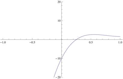
Figure 1: Plot of (4.7) with $\vec{n}=(n,m)=(1,1)$ and $\vec{\alpha}=(1/2,1/3)$.

We can also find similar counterexamples for the other choices of indices and also for multiple Laguerre polynomials of the second kind. However, multiple Laguerre polynomials satisfy the following two-parameter Turán inequalities in the sense of [17].

Theorem 4.4.

For multiple Laguerre polynomials of the first kind we have

$$L_{\vec{n}+\vec{e}_{k}}^{\vec{\alpha}}(x)L_{\vec{n}+\vec{e}_{j}}^{\vec{\alpha}-\vec{e}_{j}}(x)-L_{\vec{n}}^{\vec{\alpha}}(x)L_{\vec{n}+\vec{e}_{j}+\vec{e}_{k}}^{\vec{\alpha}-\vec{e}_{j}}(x)>0,\qquad x>0,$$ (4.8)

for $\vec{\alpha}>\vec{0}$ and $j,k=1,\ldots,r$.

Similarly, for multiple Laguerre polynomials of the second kind, we have

$$L_{\vec{n}+\vec{e}_{k}}^{(\alpha,\vec{c})}(x)L_{\vec{n}+\vec{e}_{j}}^{(\alpha-1,\vec{c})}(x)-L_{\vec{n}}^{(\alpha,\vec{c})}(x)L_{\vec{n}+\vec{e}_{j}+\vec{e}_{k}}^{(\alpha-1,\vec{c})}(x)>0,\qquad x>0,$$ (4.9)

for $\alpha>0$ and $j,k=1,\ldots,r$.

Proof.

From Theorem 1.1 with $l=2$, we see that

$$\det\begin{pmatrix}L_{\vec{n}}(x)&L_{\vec{n}+\vec{e}_{k}}(x)\\ xL_{\vec{n}}^{\prime}(x)&xL_{\vec{n}+\vec{e}_{k}}^{\prime}(x)\end{pmatrix}>0,\qquad x>0,$$ (4.10)

for $k=1,\ldots,r$, where $L_{\vec{n}}$ is the multiple Laguerre polynomial of the first or second kind. Note that $L_{\vec{n}}^{\vec{\alpha}}$ satisfies the following raising operator (cf. [35, § 23.4.2]):

$$\frac{d}{dx}\big{(}x^{\alpha_{j}}e^{-x}L_{\vec{n}}^{\vec{\alpha}}(x)\big{)}=-x^{\alpha_{j}-1}e^{-x}L_{\vec{n}+\vec{e}_{j}}^{\vec{\alpha}-\vec{e}_{j}}(x),\qquad j=1,\ldots,r,$$

or, equivalently,

$$x\frac{d}{dx}L_{\vec{n}}^{\vec{\alpha}}(x)=(x-\alpha_{j})L_{\vec{n}}^{\vec{\alpha}}(x)-L_{\vec{n}+\vec{e}_{j}}^{\vec{\alpha}-\vec{e}_{j}}(x),\qquad j=1,\ldots,r,$$

Substituting this formula into (4.10) gives us (4.8).

Similarly, (4.9) follows from (4.10) and the relation (cf. [35, § 23.4.4])

$$\frac{d}{dx}\big{(}x^{\alpha}e^{-c_{j}x}L_{\vec{n}}^{(\alpha,\vec{c})}(x)\big{)}=-c_{j}x^{\alpha-1}e^{-c_{j}x}L_{\vec{n}+\vec{e}_{j}}^{(\alpha-1,\vec{c})}(x),\qquad j=1,\ldots,r,$$

or, equivalently,

$$x\frac{d}{dx}L_{\vec{n}}^{(\alpha,\vec{c})}(x)=(c_{j}x-\alpha)L_{\vec{n}}^{(\alpha,\vec{c})}(x)-c_{j}L_{\vec{n}+\vec{e}_{j}}^{(\alpha-1,\vec{c})}(x),\qquad j=1,\ldots,r.$$

This completes the proof of Theorem 4.4. ∎

5 Configurations of zeros for the Wronskians
of multiple Hermite and Laguerre polynomials

We conclude this paper by studying numerically the geometric configuration of zeros of the Wronskians of multiple Hermite and Laguerre (of both kinds) polynomials using Mathematica. Our motivation arises from the fact that the structure of zeros of certain Wronskians of orthogonal polynomials or special functions has recently been studied numerically (cf. [19, 25, 27] and the references therein), where it is shown that they have highly regular configurations in the complex plane. It turns out that the zeros of Wronskians for certain multiple orthogonal polynomials produce intriguing pictures as well, which might be of independent interest.

Throughout this section, we take $r=2$ and denote the multi-index $\vec{n}$ by $(n,m)\in\mathbb{N}^{2}$. Unless otherwise stated, the path associated with the Wronskian (1.5) is chosen in such a way that in each step it is increased by one in the horizontal direction, i.e.,

$$(n,m)\to(n+1,m)\to(n+2,m)\to\cdots.$$

Other choices of the paths show similar behavior of the zeros. Clearly, the structure of the roots in the complex plane depends on $l$, $\vec{n}$, the path chosen and the values of the parameters, therefore, it is difficult to be described completely. We thus have chosen a few illustrative examples from numerical experiments for multiple Hermite and Laguerre polynomials to show the fascinating configurations.

5.1 Zeros of the Wronskians for multiple Hermite polynomials

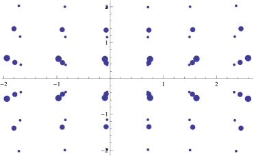
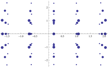
Figure 2: Zeros of the Wronskians for multiple Hermite polynomials with $\vec{n}=(3,3)$, $\vec{c}=(1/3,34/35)$ for $l=2,4,6$ (left) and $\vec{n}=(2,3)$, $\vec{c}=(1/3,2/5)$ $l=3,5,7$ (right). The size of points decreases as $l$ increases.

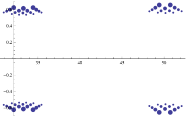
Figure 3: Zeros of the Wronskians for multiple Hermite polynomials with $\vec{n}=(2,3),(3,4),(4,5),(5,6)$, $\vec{c}=(100,=200/3)$ for $l=2$. The size of points decreases as $|\vec{n}|$ increases.

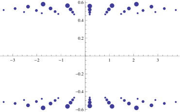
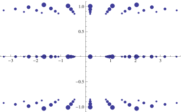
Figure 4: Zeros of the Wronskians for multiple Hermite polynomials with $\vec{n}=(2,3),(3,4),(4,5),(5,6)$ and $\vec{c}=(1/3,2/5)$ for $l=2$ (left) and $l=3$ (right). The size of points decreases as $|\vec{n}|$ increases.

The zeros of Wronskians for multiple Hermite polynomials numerically have roughly rectangular-like structure in the complex plane. In Fig. 2 we plot zeros of the Wronskians for these polynomials by fixing $\vec{n}$, the parameter $\vec{c}$ and increasing the length of the path (the size of points decreases as $l$ increases). We can see additional row of zeros on the real axis for $l$ odd, as indicated by the first part of Theorem 1.2.

If the two values in the parameter $\vec{c}$ differ too much, it seems that the zeros may separate into several rectangles, which is shown in Fig. 3 (the size of points decreases as $|\vec{n}|$ increase). When $l$ is odd, we have additional groups of zeros on the real line as projections of complex groups of roots.

The effect of increasing $|\vec{n}|$ is illustrated in Fig. 4 for $l$ even and odd respectively. As $|\vec{n}|$ increases, the zeros are distributed in a wider range. Furthermore, if $l$ increases, we can see more horizontal lines.

We illustrate Theorem 1.2 in Fig. 5. We clearly see the interlacing of real zeros and regular configurations of zeros in the complex plane. It seems that the interlacing property also appears on the other lines parallel to the real axis. For even $l$ the structure of complex roots is similar (there are no real roots in this case).

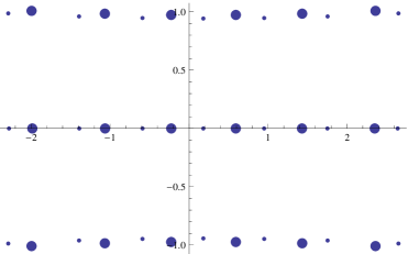
Figure 5: Theorem 1.2 for multiple Hermite polynomials with $\vec{c}=(1/3,2/5)$, $\vec{n}=(3,3)$ for $l=3$ (left) and $\vec{n}=(4,4)$ for $l=5$ (right). The size of points decreases as $|\vec{n}|$ increases.

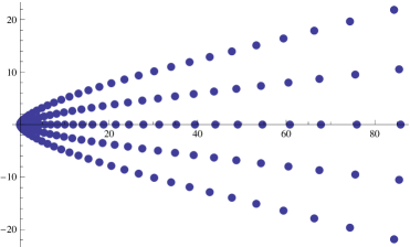
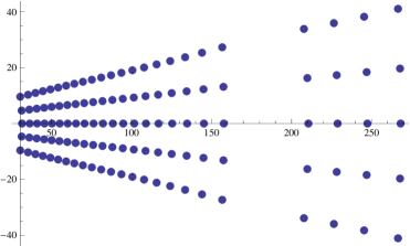
Figure 6: Zeros of the Wronskians for multiple Laguerre polynomials of the first kind with $\vec{\alpha}=(1/2,1/3)$, $\vec{n}=(10,20)$ (left) and $\vec{\alpha}=(200,200/3)$, $\vec{n}=(4,20)$ (right) for $l=5$.

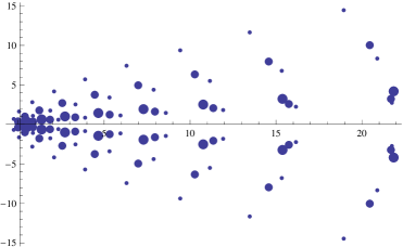
Figure 7: Zeros of the Wronskians for multiple Laguerre polynomials of the first kind with $\vec{n}=(4,5)$, $\vec{\alpha}=(1/2,1/3)$ for $l=2,4,6$. The size of points decreases as $l$ increases.

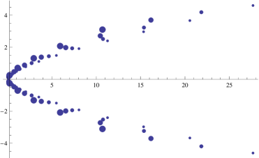
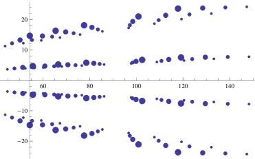
Figure 8: Zeros of the Wronskians for multiple Laguerre polynomials of the first kind with $\vec{n}=(2,3),(3,4),(4,5),(5,6)$, $\vec{\alpha}=(1/2,1/3)$ for $l=2$ (left) and $\vec{\alpha}=(100,200/3)$ for $l=4$ (right). The size of points decreases as $|\vec{n}|$ increases.

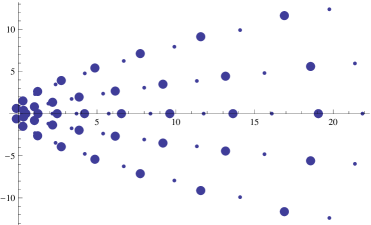
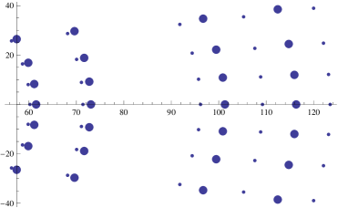
Figure 9: Theorem 1.2 for multiple Laguerre polynomials of the first kind with $\vec{n}=(4,4)$, $\vec{\alpha}=(1/2,1/3)$ for $l=5$ (left) and $\vec{n}=(2,2)$, $\vec{\alpha}=(100,200/3)$ for $l=7$ (right). The size of points decreases as $|\vec{n}|$ increases.

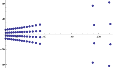
Figure 10: Zeros of the Wronskians for multiple Laguerre polynomials of the second kind with $\vec{n}=(15,2)$, $\alpha=100$, $\vec{c}=(2,3/5)$ for $l=4$.

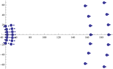
Figure 11: Theorem 1.2 for multiple Laguerre polynomials of the second kind with $\vec{n}=(2,2)$, $\alpha=100$, $\vec{c}=(2,3/5)$ for $l=7$. The size of points decreases as $|\vec{n}|$ increases.

5.2 Zeros of the Wronskians for multiple Laguerre polynomials

Since the observed structure of roots of the Wronskians for multiple Laguerre polynomials of the first and second kind is numerically quite similar, we shall concentrate more on the multiple Laguerre polynomials of the first kind. The configurations of zeros of Wronskians for multiple Laguerre polynomials of the first kind resemble (several) parabolas (with additional zeros on the real line in case $l$ is odd). Sometimes it looks like zeros lie on arcs of circles with increasing radius. As we change the parameters, we can observe that the zeros on the left can do not accumulate and, as in the case of multiple Hermite polynomials, they can be grouped into several clusters with a certain gap between them. Fig. 6 illustrates these observations.

The zeros of several Wronskians, if plotted together, also present nice interlacing properties. Following the same strategy in previous section, we fix $\vec{n}$, the parameter $\vec{\alpha}$ and increase $l$ in Fig. 7 (compare with Fig. 2), while in Fig. 8 we increase $\vec{n}$ and fix other parameters (compare with Fig. 4). Theorem 1.2 in this case is illustrated in Fig. 9.

Finally, the roots of the Wronskians for multiple Laguerre polynomials of the second kind are depicted in Fig. 10 and Theorem 1.2 is illustrated in Fig. 11.

More pictures with different configurations of roots can be found in Mathematica files on the web-pages of the authors (or available on request). We believe the nice and regular geometric configurations generated from the zeros of Wronskians deserve further analytic investigations.

Acknowledgements

We thank the referees for helpful comments, suggestions, and pointing out the additional references [23, 24, 44, 46]. LZ is partially supported by The Program for Professor of Special Appointment (Eastern Scholar) at Shanghai Institutions of Higher Learning (No. SHH1411007) and by Grant SGST 12DZ 2272800 from Fudan University. GF is supported by the MNiSzW Iuventus Plus grant Nr 0124/IP3/2011/71.

References

• [1] Abreu L.D., Bustoz J., Turán inequalities for symmetric Askey–Wilson polynomials, Rocky Mountain J. Math. 30 (2000), 401–409.
• [2] Aptekarev A.I., Asymptotics of polynomials of simultaneous orthogonality in the Angelescu case, Math. USSR Sb. 64 (1989), 57–84.
• [3] Aptekarev A.I., Multiple orthogonal polynomials, J. Comput. Appl. Math. 99 (1998), 423–447.
• [4] Aptekarev A.I., Strong asymptotics of polynomials of simultaneous orthogonality for Nikishin systems, Sb. Math. 190 (1999), 631–669.
• [5] Aptekarev A.I., Branquinho A., Van Assche W., Multiple orthogonal polynomials for classical weights, Trans. Amer. Math. Soc. 355 (2003), 3887–3914.
• [6] Baricz Á., Turán type inequalities for generalized complete elliptic integrals, Math. Z. 256 (2007), 895–911.
• [7] Baricz Á., Ismail M.E.H., Turán type inequalities for Tricomi confluent hypergeometric functions, Constr. Approx. 37 (2013), 195–221, arXiv:1110.4699.
• [8] Baricz Á., Jankov D., Pogány T.K., Turán type inequalities for Krätzel functions, J. Math. Anal. Appl. 388 (2012), 716–724, arXiv:1101.2523.
• [9] Baricz Á., Raghavendar K., Swaminathan A., Turán type inequalities for $q$-hypergeometric functions, J. Approx. Theory 168 (2013), 69–79.
• [10] Berg C., Szwarc R., Bounds on Turán determinants, J. Approx. Theory 161 (2009), 127–141, arXiv:0712.1460.
• [11] Bleher P.M., Kuijlaars A.B.J., Random matrices with external source and multiple orthogonal polynomials, Int. Math. Res. Not. 2004 (2004), no. 3, 109–129, math-ph/0307055.
• [12] Bleher P.M., Kuijlaars A.B.J., Integral representations for multiple Hermite and multiple Laguerre polynomials, Ann. Inst. Fourier (Grenoble) 55 (2005), 2001–2014, math.CA/0406616.
• [13] Brézin E., Hikami S., Level spacing of random matrices in an external source, Phys. Rev. E 58 (1998), 7176–7185, cond-mat/9804024.
• [14] Brézin E., Hikami S., Universal singularity at the closure of a gap in a random matrix theory, Phys. Rev. E 57 (1998), 4140–4149, cond-mat/9804023.
• [15] Brézin E., Hikami S., Characteristic polynomials of random matrices, Comm. Math. Phys. 214 (2000), 111–135, math-ph/9910005.
• [16] Bustamante Z., Lopes Lagomasino G., Hermite–Padé approximations for Nikishin systems of analytic functions, Sb. Math. 77 (1994), 367–384.
• [17] Bustoz J., Two-parameter Turán inequalities for ultraspherical and Laguerre polynomials, J. Math. Anal. Appl. 79 (1981), 71–79.
• [18] Chihara T.S., An introduction to orthogonal polynomials, Mathematics and its Applications, Vol. 13, Gordon and Breach Science Publishers, New York – London – Paris, 1978.
• [19] Clarkson P.A., The fourth Painlevé equation and associated special polynomials, J. Math. Phys. 44 (2003), 5350–5374.
• [20] Csordas G., Norfolk T.S., Varga R.S., The Riemann hypothesis and the Turán inequalities, Trans. Amer. Math. Soc. 296 (1986), 521–541.
• [21] Delvaux S., Average characteristic polynomials for multiple orthogonal polynomial ensembles, J. Approx. Theory 162 (2010), 1033–1067, arXiv:0907.0156.
• [22] Durán A.J., Wronskian type determinants of orthogonal polynomials, Selberg type formulas and constant term identities, J. Combin. Theory Ser. A 124 (2014), 57–96, arXiv:1207.4331.
• [23] Elbert Á., Laforgia A., Some monotonicity properties of the zeros of ultraspherical polynomials, Acta Math. Hungar. 48 (1986), 155–159.
• [24] Elbert Á., Laforgia A., Monotonicity results on the zeros of generalized Laguerre polynomials, J. Approx. Theory 51 (1987), 168–174.
• [25] Felder G., Hemery A.D., Veselov A.P., Zeros of Wronskians of Hermite polynomials and Young diagrams, Phys. D 241 (2012), 2131–2137, arXiv:1005.2695.
• [26] Filipuk G., Van Assche W., Zhang L., Ladder operators and differential equations for multiple orthogonal polynomials, J. Phys. A: Math. Theor. 46 (2013), 205204, 24 pages, arXiv:1204.5058.
• [27] Forrester P.J., Rains E.M., A Fuchsian matrix differential equation for Selberg correlation integrals, Comm. Math. Phys. 309 (2012), 771–792, arXiv:1011.1654.
• [28] Gantmacher F.R., The theory of matrices. Vol. 1, Chelsea Publishing Co., New York, 1959.
• [29] Gasper G., An inequality of Turán type for Jacobi polynomials, Proc. Amer. Math. Soc. 32 (1972), 435–439.
• [30] Gasper G., On two conjectures of Askey concerning normalized Hankel determinants for the classical polynomials, SIAM J. Math. Anal. 4 (1973), 508–513.
• [31] Gautschi W., Orthogonal polynomials: computation and approximation, Numerical Mathematics and Scientific Computation, Oxford Science Publications, Oxford University Press, New York, 2004.
• [32] Gonchar A.A., Rakhmanov E.A., Sorokin V.N., On Hermite–Padé approximants for systems of functions of Markov type, Sb. Math. 188 (1997), 671–69.
• [33] Haneczok M., Van Assche W., Interlacing properties of zeros of multiple orthogonal polynomials, J. Math. Anal. Appl. 389 (2012), 429–438, arXiv:1108.3917.
• [34] Hua L.K., Harmonic analysis of functions of several complex variables in the classical domains, Amer. Math. Soc., Providence, R.I., 1963.
• [35] Ismail M.E.H., Classical and quantum orthogonal polynomials in one variable, Encyclopedia of Mathematics and its Applications, Vol. 98, Cambridge University Press, Cambridge, 2005.
• [36] Ismail M.E.H., Determinants with orthogonal polynomial entries, J. Comput. Appl. Math. 178 (2005), 255–266.
• [37] Ismail M.E.H., Laforgia A., Monotonicity properties of determinants of special functions, Constr. Approx. 26 (2007), 1–9.
• [38] Karlin S., McGregor J.L., Determinants of orthogonal polynomials, Bull. Amer. Math. Soc. 68 (1962), 204–209.
• [39] Karlin S., Szegő G., On certain determinants whose elements are orthogonal polynomials., J. Analyse Math. 8 (1960), 1–157.
• [40] Kershaw D., A note on orthogonal polynomials, Proc. Edinburgh Math. Soc. 17 (1970), 83–93.
• [41] Krasikov I., Turán inequalities for three-term recurrences with monotonic coefficients, J. Approx. Theory 163 (2011), 1269–1299, arXiv:1101.3204.
• [42] Kuijlaars A.B.J., Multiple orthogonal polynomial ensembles, in Recent Trends in Orthogonal Polynomials and Approximation Theory, Contemp. Math., Vol. 507, Editors J. Arvesú, F. Marcellán, A. Martínez-Finkelshtein, Amer. Math. Soc., Providence, RI, 2010, 155–176, arXiv:0902.1058.
• [43] Kuijlaars A.B.J., Multiple orthogonal polynomials in random matrix theory, in Proceedings of the International Congress of Mathematicians. Vol. III, Hindustan Book Agency, New Delhi, 2010, 1417–1432, arXiv:1004.0846.
• [44] Laforgia A., Sturm theory for certain classes of Sturm–Liouville equations and Turánians and Wronskians for the zeros of derivative of Bessel functions, Indag. Math. 86 (1982), 295–301.
• [45] Leclerc B., On certain formulas of Karlin and Szegö, Sém. Lothar. Combin. 41 (1998), Art. B41d, 21 pages.
• [46] Lorch L., Turánians and Wronskians for the zeros of Bessel functions, SIAM J. Math. Anal. 11 (1980), 223–227.
• [47] Mehta M.L., Normand J.M., Moments of the characteristic polynomial in the three ensembles of random matrices, J. Phys. A: Math. Gen. 34 (2001), 4627–4639, cond-mat/0101469.
• [48] Nikishin E.M., Sorokin V.N., Rational approximations and orthogonality, Translations of Mathematical Monographs, Vol. 92, Amer. Math. Soc., Providence, RI, 1991.
• [49] Nuttall J., Wronskians, cumulants, and the Riemann hypothesis, Constr. Approx. 38 (2013), 193–212.
• [50] Skovgaard H., On inequalities of the Turán type, Math. Scand. 2 (1954), 65–73.
• [51] Szász O., Inequalities concerning ultraspherical polynomials and Bessel functions, Proc. Amer. Math. Soc. 1 (1950), 256–267.
• [52] Szász O., Identities and inequalities concerning orthogonal polynomials and Bessel functions, J. Analyse Math. 1 (1951), 116–134.
• [53] Szegő G., On an inequality of P. Turán concerning Legendre polynomials, Bull. Amer. Math. Soc. 54 (1948), 401–405.
• [54] Szegő G., Orthogonal polynomials, American Mathematical Society, Colloquium Publications, Vol. 23, 4th ed., Amer. Math. Soc., Providence, R.I., 1975.
• [55] Turán P., On the zeros of the polynomials of Legendre, Časopis Pěst. Mat. Fys. 75 (1950), 113–122.
• [56] Van Assche W., Multiple orthogonal polynomials, irrationality and transcendence, in Continued Fractions: from Analytic Number Theory to Constructive Approximation (Columbia, MO, 1998), Contemp. Math., Vol. 236, Amer. Math. Soc., Providence, RI, 1999, 325–342.
• [57] Van Assche W., Padé and Hermite–Padé approximation and orthogonality, Surv. Approx. Theory 2 (2006), 61–91, math.CA/0609094.
• [58] Van Assche W., Coussement E., Some classical multiple orthogonal polynomials, J. Comput. Appl. Math. 127 (2001), 317–347, math.CA/0103131.
• [59] Vermes R., On Wronskians whose elements are orthogonal polynomials, Proc. Amer. Math. Soc. 15 (1964), 124–126.
• [60] Zinn-Justin P., Universality of correlation functions of Hermitian random matrices in an external field, Comm. Math. Phys. 194 (1998), 631–650, cond-mat/9705044.
\LastPageEnding