Generation and Transfer of Polarized Radiation
in Hydrodynamical Models of the
Solar Chromosphere.

Examination date: December 2013.
Thesis supervisors:
Dr. Andrés Asensio Ramos & Prof. Javier Trujillo Bueno

©  Edgar S. Carlin Ramírez, 2024
ISBN: xx-xxx-xxxx-x
Depósito legal: TF-1207/2013


Some of the material included in this document has been already published in The Astrophysical Journal.
Parte del material incluido en este documento ya ha sido publicado en The Astrophysical Journal.

Resumen

El principal objetivo de esta tesis ha sido investigar el efecto que los gradientes de velocidad vertical tienen en las señales de polarización por scattering formadas en la cromosfera solar. Seguimos un enfoque teórico basado en la síntesis espectral de señales de polarización en modelos dinámicos del Sol en calma. Los movimientos macroscópicos nunca habían sido considerados en el tratamiento de señales de polarización producidas por procesos de scattering y efecto Hanle. Esto es especialmente importante en la cromosfera solar, dado su fuerte dinamismo y su reducida intensidad de campo magnético. El estudio se centra en el análisis de las líneas del triplete infrarrojo del Ca ii (en $8498$, $8542$ y $8662$ Å). La metodología de síntesis de perfiles de Stokes permite confrontar los modelos cromosféricos con observaciones.

Resolvimos el problema NLTE del transporte y generación de radiación polarizada en sistemas atómicos multinivel usando modelos de atmósfera solar con creciente nivel de realismo: atmósferas Milne-Eddington, atmósfera compuesta por átomos de dos niveles, modelos semiempíricos con velocidades ad-hoc, series temporales de modelos hidrodinámicos y una captura instantánea de una simulación MHD tridimensional. Para ello incluimos la acción de los campos de velocidad sobre la polarización atómica. Primero estudiamos el impacto de los gradientes de velocidad en la anisotropía del campo de radiación, la cual controla la polarización por scattering; luego mostramos los efectos de modulación en amplitud, desplazamiento espectral y asimetrización que los gradientes de velocidad vertical y las ondas de choque cromosféricas producen sobre los perfiles de de polarización lineal a campo cero; finalmente, estudiamos la polarización emergente en geometría de forward scattering incluyendo el efecto Hanle producido por el campo magnético.

Así sintetizamos la primera tomografía de un modelo de la cromosfera de Sol en calma que combina mapas de polarización por scattering y efecto Hanle junto con mapas de polarización circular producidos por efecto Zeeman. Nos centramos en el uso de estos mapas para el diagnóstico de la topología espacial del campo magnético, del estado termodinámico de la atmósfera y de la estratificación de velocidades. Estudiamos también la relevancia de la termodinámica y la dinámica en el cálculo de la orientación del campo magnético en presencia de las ambigüedades de $90\,\mbox{${}^{\circ}$}$ y $180\,\mbox{${}^{\circ}$}$. Además, simulamos observaciones degradando los mapas de polarización resultantes tal y como haría el futuro telescopio espacial Solar-C con observaciones reales, reconstruyéndolas posteriormente mediante varios métodos (por ejemplo, PCA). Encontramos que Solar-C y EST deberían ser capaces de medir comportamientos similares a los simulados en esta tesis para el triplete IR del Ca ii.

Dedicamos un capítulo a las herramientas y procedimientos técnicos desarrollados: códigos de transporte radiativo, método de adaptación de redes numéricas para mejorar la convergencia de los códigos de transporte, código de análisis de componentes principales, herramienta de cálculo de funciones respuesta en líneas cromosféricas y técnicas de visualización y análisis tridimensional.

Summary

The main goal of this thesis has been to investigate the effect that the macroscopic vertical velocity fields have on the scattering polarization signals formed in the solar chromosphere. We followed a theoretical approach based on the spectral synthesis of scattering polarization signals in dynamic models of the quiet Sun. Until now, the impact of macroscopic motions had never been considered in the treatment of the polarization signals produced by scattering processes and the Hanle effect. This is especially important in the solar chromosphere, given its strong dynamism and reduced magnetic field intensity. This investigation focuses in the analysis of the Ca ii IR triplet lines (at $8498$, $8542$ and $8662$ Å). The methodology of spectral synthesis allows to confront chromospheric models with real observations.

We solved the multilevel, non-LTE radiative problem of the generation and transfer of polarized radiation in increasingly realistic atmosphere models: Milne-Eddington atmospheres, atmospheres composed by two-level atoms, semiempirical models with ad-hoc velocities, hydrodynamical time-dependent models and a snapshot of a 3D MHD simulation. To such end, we included the action of the velocity fields on the atomic level polarization. Thus, we studied the impact of velocity gradients on the anisotropy of the radiation field, which controls the scattering polarization. We showed the effects of amplitude modulation, spectral shift and asymmetry that the vertical velocity gradients have on the zero-field linear polarization profiles; finally, we studied the emergent polarization in a forward scattering geometry including as well the Hanle effect produced by the magnetic field.

Thus, we obtained the first tomographic view of a model quiet chromosphere that includes synthetic maps of linear polarization dominated by Hanle effect and of circular polarization dominated by Zeeman effect. We focused on the use of such maps to diagnose the spatial topology of the magnetic field, the thermodynamical state of the atmosphere and the vertical stratification of velocity. We also studied the relevance of dynamic and thermodynamic in the calculation of the chromospheric magnetic field orientation in the presence of the $90\,\mbox{${}^{\circ}$}$ and $180\,\mbox{${}^{\circ}$}$ ambiguities. Furthermore, we simulated synthetic observations by degrading our polarization maps, as the space telescope Solar-C would do with real observations, and we reconstructed them by following several methods (e.g., Principal Component Analysis). We found that Solar-C and the European Solar Telescope should be able to capture bevaviors similar to the ones simulated in this thesis for the Ca ii IR triplet lines.

We dedicated a chapter to the tools and technical procedures developed in this thesis: the RT code; an adaptative method for numerical grids that improves the convergence of the RT calculation; a PCA code; a program to calculate response functions for chromospheric lines; and finally, some techniques for three-dimensional analysis and visualization.

Contents

1. Resumen
2. Summary
3. 1 Introduction
4. 2 Spectral line polarization in stellar atmospheres
   1. 2.1 Radiative transfer with polarization.
      1. 2.1.1 Quantum mechanical description
      2. 2.1.2 The radiative transfer equation
      3. 2.1.3 Line broadening mechanisms
      4. 2.1.4 Radiative transfer coefficients
      5. 2.1.5 Statistical equilibrium equations
      6. 2.1.6 Radiation field.
   2. 2.2 Numerical methods for polarized radiative transfer.
      1. 2.2.1 Integration of the transfer equation.
      2. 2.2.2 Statement of the iterative problem.
      3. 2.2.3 Iterative scheme.
      4. 2.2.4 Evaluation of $\Lambda^{*}$
   3. 2.3 Line formation in moving atmospheres
      1. 2.3.1 Effect of the velocity on the radiative transfer.
      2. 2.3.2 Effect of the velocity in the SEE.
      3. 2.3.3 Effect of the velocity on the atomic density matrix.
   4. 2.4 The Hanle Effect in the solar atmosphere
      1. 2.4.1 Description
      2. 2.4.2 A hands-on guide to the Hanle equations
      3. 2.4.3 Hanle effect at work: two examples.
5. 3 Developed tools and methodology.
   1. 3.1 A RT code for dynamic scattering polarization.
      1. 3.1.1 Traviata.
      2. 3.1.2 The new version of Traviata
      3. 3.1.3 A FEM-based optimization method for the spatial grid.
   2. 3.2 Response functions in chromospheric solar models.
   3. 3.3 Tools for Principal Component Analysis.
   4. 3.4 The Solar Inspector
   5. 3.5 Advanced 3D visualization with Mayavi.
6. 4 Scattering Polarization with Velocity Gradients.
   1. 4.1 Introduction
   2. 4.2 Formulation of the problem and relevant equations
      1. 4.2.1 The atomic model and the statistical equilibrium equations (SEE)
      2. 4.2.2 The radiative transfer equations (RTE)
      3. 4.2.3 Numerical method
   3. 4.3 Effect of a velocity gradient on the radiation field.
      1. 4.3.1 Anisotropy seen by a moving scatterer.
      2. 4.3.2 Calculations in a Milne-Eddington model.
      3. 4.3.3 Two-level model atom in dynamic atmospheres.
   4. 4.4 Results for the Ca ii IR Triplet
      1. 4.4.1 Behavior of the anisotropy in the Ca ii IR triplet
      2. 4.4.2 The impact of the emergent radiation on the polarization.
      3. 4.4.3 Variations on the atomic alignment due to velocity gradients.
   5. 4.5 Conclusions
7. 5 Scattering Polarization of the Ca ii IR triplet in Hydrodynamical Models
   1. 5.1 Description of the problem and the resolution procedure.
   2. 5.2 Description and characterization of the results.
   3. 5.3 Analysis and discussion of results.
      1. 5.3.1 The effect of the velocity.
      2. 5.3.2 The combined effect of velocity and temperature on the linear polarization.
      3. 5.3.3 Averaged values of the polarization profiles.
      4. 5.3.4 The velocity free approximation.
      5. 5.3.5 The effect of photospheric dynamics.
      6. 5.3.6 The effect of the integration time.
      7. 5.3.7 The effect of a decreasing velocity on the averaged profiles.
   4. 5.4 Considerations on the Hanle effect
   5. 5.5 Conclusions
8. 6 Synthesis of Stokes profiles in a 3D MHD atmospheric model.
   1. 6.1 Description of the MHD model and the RT calculations.
      1. 6.1.1 Pre-processing the models.
      2. 6.1.2 Description of physical quantities in the model.
   2. 6.2 Synthetic polarization profiles in forward scattering.
      1. 6.2.1 Individual profiles.
      2. 6.2.2 Slit profiles.
   3. 6.3 Maps of radiative quantities.
      1. 6.3.1 Maps of polarization amplitudes.
      2. 6.3.2 The Hanle Polarity Inversion Lines.
      3. 6.3.3 Maps of the Polarization Degree.
      4. 6.3.4 Maps of polarization contrasts.
   4. 6.4 Effect of the vertical velocities.
   5. 6.5 Synthetic observations.
      1. 6.5.1 The space telescope Solar- C.
      2. 6.5.2 Degraded and restored maps of Polarization Amplitudes.
      3. 6.5.3 Degraded and restored maps of the Linear Polarization Degree.
      4. 6.5.4 The practical disadvantages of the typical spectropolarimetric quantities.
      5. 6.5.5 Reconstruction with PCA methods.
   6. 6.6 Spectropolarimetric inference of the magnetic field.
      1. 6.6.1 The Zeeman effect and the weak field approximation.
      2. 6.6.2 Magnetic Field Direction and Ambiguities in the Hanle regime.
      3. 6.6.3 The disambiguation process.
      4. 6.6.4 Magnetic field intensity.
9. 7 Conclusions and future work
   1. 7.1 Goals achieved
   2. 7.2 Conclusions
   3. 7.3 Future work
10. A Appendix.
    1. A.1 Special functions in section 4.3.1
    2. A.2 Statistical equilibrium equations in the non-magnetic case.
    3. A.3 Derivation of the fractional linear polarization under EB approximation.
    4. A.4 Other figures in Chapter 6.
    5. A.5 Stereographic view of a cool chromospheric bubble.
11. Agradecimientos

Chapter 1 Introduction

In $1892$, Charles A. Young wrote (Young, 1862):

“…This outer envelope…seems to be made up not of overlying strata of different density, but rather of flames, beams and streamers, as transient as those of our own aurora borealis. It is divided into two portions…the outer portion…may almost, without exaggeration, be likened to ’the stuff that dreams are made of’, since it is chiefly due to the ’corona’ or glory which surrounds the darkened Sun during an eclipse… At its base, and in contact with the photosphere, is what resembles a sheet of scarlet fire… This is the ’chromosphere’ …”

These annotations already gave a clear qualitative description of the outer layers of the solar atmosphere, containing also one of the first scientific reports of what today is known as a chromospheric emission. Beginning in the famous Indian eclipse of 1868 August 18, the application of the yet novel spectroscopic visual techniques to the Sun started to reveal several crucial facts about its physical properties. They would also constitute the basis for the flourishment of the present astrophysical spectropolarimetry.

Irrespective of the scientific explanations we could give, the vision of our moon exactly matching the Sun’s circumference will never cease to be amazing (Figure 1.1, left panel). But better eyes to observe it are always welcome. Thanks to the instrumental works of Secchi in the 1860s and to the subsequent establishment of a proper observational methodology, the increasing interest and fascination of the scientists for the solar atmosphere transformed it in a very attractive topic of research. Besides the identification of the main outer regions of the Sun, the incipient spectroscopy allowed their composition to be measured. Scientists like Herschel, Rayet, and Janssen realized that the faint glow of the chromosphere was due to an emission spectrum from hot, low density gases emitting at discrete wavelengths, the “scarlet fire” being due to the strong Balmer H$\alpha$ emission (Figure 1.1, middle panel). Also through spectroscopic methods, the discovery of the second most abundant element in the universe, helium, was first done in emission lines seen in the solar chromosphere during that Indian eclipse of 1868 (helium was not found on Earth until 1895!).

At that time, the chromosphere could only be distinguished easily during a total solar eclipse because it glows faintly relative to the photosphere. But the invention of the first spectroheliograph by Hale and Deslandres (1890) allowed the study of the solar disk chromosphere at any time. It led Hale to reveal the “chromospheric network” at various wavelengths in the Ca ii H and K lines and in H$\beta$, and showed that enhanced chromospheric emission occurs in “clouds” or “flocculi” above photospheric faculae (Hale & Ellerman, 1904). These regions are overlaid and mixed with ubiquitous hair-like fine structures, later termed “jets” or “spicules” when they are seen at the limb, or “mottles” when seen on disk. Hale (Hale & Adams, 1909) also obtained the first spectroheliograms of the disk in H$\alpha$, which revealed that “…is clearly visible on the hydrogen photographs. It is a decided definiteness of structure indicated by radial or curving lines, or as some such distribution of the minor flocculi as iron filings present in a magnetic field”. Thus, together with the discovery of the Zeeman effect in sunspots (Hale, 1908), Hale had confirmed a stunning and essential fact: the magnetic nature of the Sun (figure 1.1).

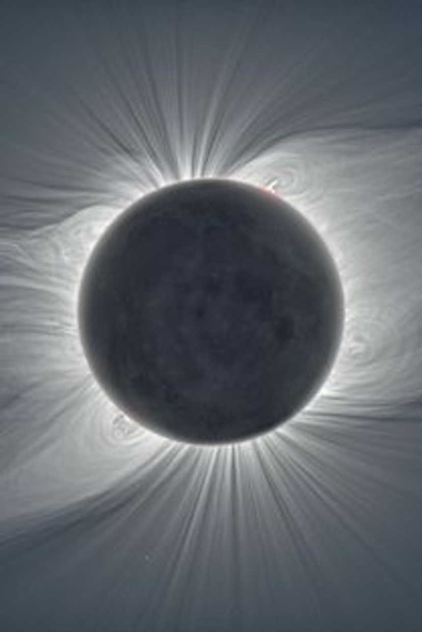
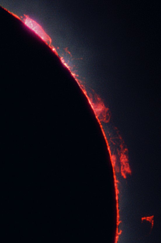
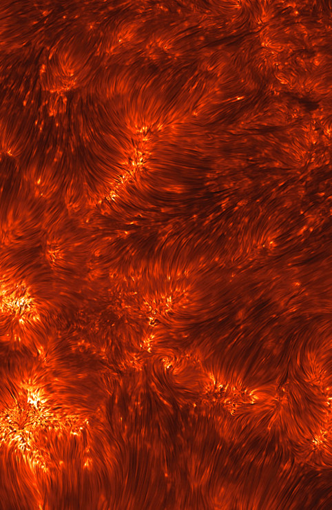
Figure 1.1: Left: Coronal magnetic fields (’the stuff that dreams are made of’) during the solar eclipse of 2008. Center: chromospheric emission at the solar limb during a total eclipse. Right: Fibrilar structures (spicules or mottles) in H$\alpha$. They trace network (brighter) and internetwork (darker) areas at the solar disk.

The magnetic field plays a crucial role in the behavior of the solar atmosphere. It is one of the three main drivers defining the chromosphere (together with dynamics and thermodynamics). Indeed, its importance in Astrophysics is universal. To explain it, we can first consider the symmetry between electric and magnetic fields in the Maxwell equations describing the propagation of electromagnetic waves. They are symmetric in their interactions. On the contrary, there is a lack of symmetry between the sources (charges) of the electric and magnetic fields in such equations. Effectively, the matter throughout the cosmos is found to consist only of electrically charged particles, i.e., electrons and nucleons, with no indicia of scalar magnetic sources (magnetic monopoles). On the other hand, since most of the gases in the universe are at least partially ionized, there is an abundance of free electrons and ions. Hence, a consequence of these facts is that an electric current density can be easily created by a very weak electric field, quickly reducing to negligible values any large-scale electric field in the reference frame of the moving plasma. In other words, the abundance of free charges shortcircuits the electric fields very fast, leaving the universe impregned only by the magnetic field at large distances (Parker, 2007). At the same time, charges in motion with respect to an external observer, are themselves sources of seed magnetic fields that are amplified by rotation and convection in the stars (as stated by the induction equation in MHD theory). That is one of the basis of the solar dynamo mechanism (Charbonneau, 2010). The stellar magnetic fields are then created and driven by organized macroscopic relative motions between electric charges in the plasma. In the absence of motions, the most notable chromospheric and coronal structures, such as those spicules or the longer “iron fillings” described by Hale, would not exist.

In relation with the outer solar layers, it is believed that the dissipation of magnetic energy in the $10^{6}$ K corona may be significantly modulated by the strength and structure of the magnetic field in the chromosphere (e.g., Parker, 2007). According to the variation of the magnetic field with height in the Sun, the chromosphere is an interface layer lying between the gas-dominated photosphere (where field lines are frozen in the plasma, dragged about by surface flows) and the field-dominated corona (where the ionized plasma is forced to flow along the field lines). At such extremes the field adopts the form of small-scale intense flux tubes in the high-$\beta$ photosphere and produces loop-like structures in the low-$\beta$ corona. In the middle, magnetic fields can be highly twisted and tangled, being expanded from below to fill the chromosphere.

The structure of the chromosphere is thus determined by the magnetic field, while its dynamics is dominated by oscillations and flows arriving amplified from the convective photosphere. Indeed, dynamics is specially important in the solar chromosphere because of the much larger velocities existing there in comparison with the photosphere. The combination of intricate structure on small scales and fast dynamics make the chromosphere one of the most defying regions for the comprehension of the solar atmosphere. Some problems are the channelling of the highly conducting and partially ionized plasma through the field lines, and the changing of the force balance ($\beta$ parameter) within the chromosphere, which leads to drastic variations in field morphology and wave mode propagation. The magnetic field dramatically changes the ways energy can be transported and dissipated, compared with the field-free case. Figure 1.2 sketches some of the complications introduced by magnetic fields and dynamics (Judge, 2006).

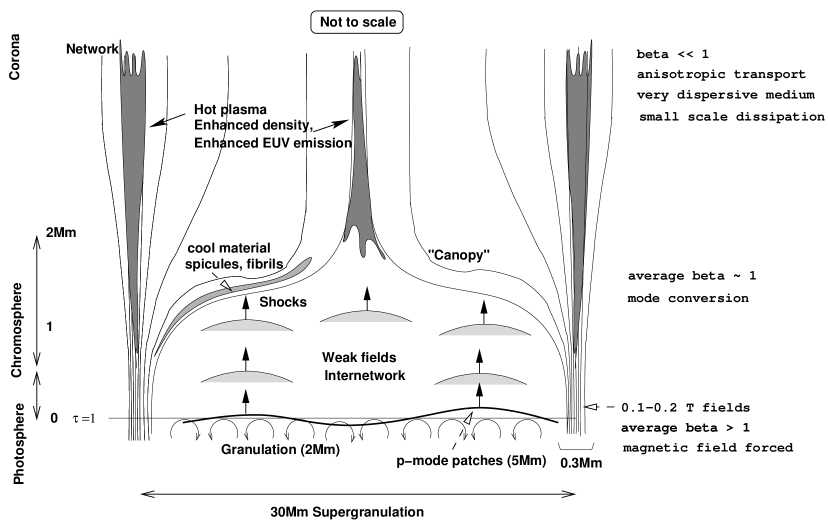
Figure 1.2: Schematic picture of the structure of the solar chromosphere in a quiet-Sun unipolar magnetic field region. From Judge (2006).

In particular, the turbulent nature of the underlying photosphere will inevitably lead to magnetic free energy (current systems) throughout the entire atmosphere. It basically consists in very small scale current sheets and dissipation regions below the current observable scales (Parker, 1994). Thus, the combination of magnetic fields and dynamics, which includes shocks and turbulence, leads to an atmospheric “global warming”.

The temperature profile is the third distinctive attribute commonly used to define the solar chromosphere. In this region, most of the non-thermal energy that creates the corona and the solar wind is released, with a heating rate requirement that is between one and two orders of magnitude larger than in the corona (Ayres et al., 2009). In quiet Sun regions, the chromosphere extends from the temperature minimum at about $500$ km to the sudden steep increase around $2100$ km (the transition region to the corona, where temperature changes from $10^{4}$ K to $10^{6}$ K). The nature of the chromospheric temperature rise is still unclear. Acoustic waves have long been proposed as the main energy source that heats the quiet-Sun chromosphere. They steepen into shocks as they propagate upward in the atmosphere, heating it as they dissipate. This would produce a highly time-dependent heating (e.g., Carlsson & Stein, 2002).

In the last instance, only one driver alters the chromosphere at all scales: dynamics. Motions of charges generate and sustain the fields; macroscopic motions in plasmas can transport and distort the fields, or can alter the optical properties of the fluid; and even temperature is a proxy for microscopic motions.

To observationally understand the information that we receive from the chromosphere, it is also important to discriminate what we are looking at. Since the visual work of Secchi in the 1870s to the impressive satellite pictures of today, the observational appearance of the chromosphere has always shown the remarkable and beautiful fine structure that seems to predominate (figure 1.1, right panel). It is then easy to imagine a chromosphere mostly composed by those streamers of plasma (spicules) that Charles A. Young pointed out.

But, contrarily to that first impression, most of the mass in the chromosphere have to be disposed in gravitationally stratified layers of plasma, not in spicules defying gravity (Judge, 2010). We have here to distinguish between the fine-structured chromosphere and the ambient chromosphere from which spicules originate. The chromosphere fibrilar structure bears similarities in morphology and dynamics to the overlying corona, being a kind of conspicuos interface layer. When observing with broadband filters, the instruments preferentially detect those bright, dynamic jets whose line widths and Doppler shifts are sufficient to avoid the absorption by the intervening material (Judge & Carlsson, 2010). Thus, the “non-spicule” chromosphere, which in any case must be present to account for material with significant opacity in the Ca II lines (Lites et al., 1993), cannot be easily seen in the observations. Today we know that spicules have far smaller filling factor and density (by several orders of magnitude) than the chromospheric pool.

A signature property of such ambient chromosphere pointed out before is its geometrical extension (near ten pressure scale heights), which is much larger than expected in a hydrostatic atmosphere where gravity is balanced by pressure gradients. During a long time the question was: which are the forces balancing the chromospheric stratification? In the past, the two competing solutions were a hydrostatically stratified chromosphere supported on radiation-pressure gradients (Milne, 1924), and a similar model whose extra support was given by turbulence instead of radiation (McCrea, 1929). It was not until the middle of the twentieth century that the development of the radiation transfer and spectral line formation theory started to include the extreme departures from classical Local Thermodynamic Equilibrium (LTE) at the very low densities and high temperatures of the chromospheric regions. The solution inclined favourably to Milne’s model, and the discussion led to the introduction of Non-LTE effects for explaining the observations. Years later, Athay & Thomas (1961) concluded that, including NLTE effects, a hydrostatically stratified distribution of plasma is in good agreeement with the limb observations made in the continuum. They also showed that in NLTE, the dependence of ionization equilibrium on electron pressure still naturally produces higher ionization stages at higher layers in stratified media, as Saha (1920) found assuming LTE. Several decades of research on chromosheric lines have redounded in a well-established line formation theory able to model chromospheric spectral lines under NLTE conditions (e.g., the monographs by Mihalas, 1978; Cannon, 1985; Rutten, 2003).

Today, the large extent of the chromosphere is explained in terms of ionization of its dominant constituent, hydrogen. Given its large ionization potential, hydrogen acts as a sponge that soaks up energy, buffering the gas to some degree from local heatings (like acoustic shocks) and moderating the temperatures (Ayres et al., 2009). The key point is that ionization frees electrons to feed regular and continuous cooling by collisional excitation and subsequent radiative de excitation of abundant species such as Feii, Mgii and Caii. The radiative cooling produced by those lines is a signature property of the chromosphere. This “ionization valve” works effectively along many scale heights because of the large dynamic range of the electron fraction, $\mathrm{n_{e}/n_{H}}$. It is only $10^{-4}$ at the base of the chromosphere (where the electrons are from singly ionized metals), but at the top it approaches unity (hydrogen mostly ionized). This allows considerable margin for the gas to balance heating even while the overall density falls outward (Ayres, 1979). Once the pool of neutral hydrogen is exhausted, the valve cannot continue to balance the heating and a thermal escape could propagate towards the corona. This scenario is appealing to explain the large extent and the “thermostat” role of solar-like chromospheres but, for the moment, it is not enough to fully explain the so-called coronal heating problem. To solve this and other various problems we have to engage more pieces of the puzzle. How do we connect the physical properties of the chromosphere with the observed spectral line radiation? This thesis is about the answer to that question.

To validate and test the link between theory and observations, a reliable diagnostic technique should be able to accomodate the influence of magnetic field, temperature and velocity, while guided by a detailed line formation theory.

On one hand, the scattering in strong resonance transitions feeded by the hydrogen ionization becomes a dominant energy transport mechanism (radiative cooling). The nonlocality of such radiation fields, induced by the lower opacity in higher layers, creates serious challenges for remote sensing that have to be solved with the help of theoretical and numerical approximations to the radiative transfer problem.

On the other hand, “measuring” the chromospheric magnetic field is notoriously difficult (e.g., reviews by Casini & Landi Degl’Innocenti, 2007; Harvey, 2009; Trujillo Bueno, 2010). While spectroscopic observations allow us to determine temperatures, flows and waves, they do not provide any quantitative information on the chromospheric magnetic field. To this end, we need to measure and interpret the polarization that some physical mechanisms introduce in chromospheric spectral lines. From Maxwell’s electromagnetic wave theory it follows that the spectral radiation is characterized by its intensity and also by its polarization, which is defined in the plane perpendicular to the direction of propagation of the light ray (the transversal plane). G. G. Stokes showed how intensity and polarization could be described in a unified way by the Stokes 4-vector. The first vector component represents the ordinary intensity (I), the second and third components (Q and U) describe linear polarization along two reference directions in the transversal plane, while the fourth component (V) relates to the circular polarization. This is a very powerful way to describe any partially polarized light beam while giving all the four vector components in the same (intensity) units (Born & Wolf, 1980). In practice, this representation implies that spectropolarimetry is actually differential photometry. The difference between the number of photons oscillating in one reference direction along the transversal plane and the number of photons oscillating perpendicularly in the same plane gives Stokes Q and U. Something similar holds for Stokes V, which is the difference between right-handed and left-handed circularly polarized photons. Going from spectroscopy to spectropolarimetry thus means an increment in the dimensionality of information space from 1-D to 4-D. Hence, in polarized radiative transfer (RT), instead of a scalar problem we have to deal with the transfer of a 4-vector. This increases the richness but also the complexity of the physical situation. It is the price to pay for getting access to stellar magnetic fields.

Historically, the discovery of the magnetic effects on the light was guided by laboratory experiments. In $1896$, Pieter Zeeman, disobeying the direct orders of his supervisor, used laboratory equipment to measure the action of a strong magnetic field on spectral lines. Thus, he discovered his homonymous effect, consisting in the splitting of a spectral line into several polarized components by the action of a static magnetic field.

The circular and linear polarization signals that the Zeeman effect can produce in a spectral line are caused by the wavelength shifts between the so-called $\pi$ and $\sigma$ transitions of the line (Zeeman splitting) induced by the presence of a magnetic field. The amplitude of the circular polarization scales with the ratio $\cal R$ between the Zeeman splitting and the Doppler line width. The amplitude of the linear polarization scales with ${\cal R}^{2}$ (see Landi Degl’Innocenti & Landolfi, 2004). Outside sunspots (where $B\,{\lesssim}\,100$ G at chromospheric heights) ${\cal R}{\ll}1$, which explains why it is so difficult to detect the linear polarization of the Zeeman effect in a chromospheric line. Typically, only the Zeeman circular polarization is detected, especially in long-wavelength chromospheric lines such as those of the IR triplet of Caii (e.g., Trujillo Bueno, 2010, Figure 3). Then, the linear polarization observed in quiet regions of the solar chromosphere has practically nothing to do with the transverse Zeeman effect.

On the other hand, in 1922 Wood and Ellett published a paper describing the effect of a magnetic field on the polarization of resonance fluorescence radiation emitted by a cell of mercury vapor. It turned out that a constant magnetic field of a few gauss was sufficient to depolarize the scattered radiation. Wood and Ellett soon realized that this behavior could not be interpreted as a Zeeman effect since the Zeeman separation in such fields was very small compared to the typical Doppler-broadened linewidth of such radiation. In $1924$ Hanle gave a classical explanation of the effect arguing that the external magnetic field produces, due to the Lorentz force, a precession of the atom electrons about the field direction. Such precession breaks the linear pattern of the oscillations re-emitted by the atoms and leads to a depolarized detected radiation. Attempts to better understand the phenomenon were important in the subsequent development of quantum physics.

It was through spectropolarimetry that measurements of stellar magnetic fields became possible: first, with the works of Hale (remember, the spectroheliograph’s inventor who detected the Zeeman effect in intensity while studying sunspots), and Babcock (1947), who succesfully measured the circularly polarized Zeeman components on stars; much later on, with the pioneering works of Omont et al. (1973); Bommier & Sahal-Bréchot (1978) and Stenflo (1978), the Hanle effect was studied in the context of the radiative transfer and measured in the solar atmosphere (Stenflo, 2013).

Polarization is related to some symmetry breaking process. For instance, in the case of the Zeeman effect, the spatial symmetry breaking induced by the magnetic field is transferred to the radiation as an asymmetry between the orientation sense of the circularly polarized blue and red sigma components. In a non-magnetized atmosphere, the symmetry can be broken by a scattering process, depending on the angles between the incident and scattered radiation. Similarly to the light emitted from the Earth sky, which is linearly polarized by molecular Rayleigh scattering, the solar spectrum is linearly polarized by scattering processes in the Sun’s atmosphere. In weakly magnetized regions, the linear polarization of chromospheric lines is dominated by scattering processes. The geometrical distribution of the solar atmospheric structures can create, simply by the lack of symmetry in the illumination they produce, a phase relationship between the excitation and emission processes in scattering atoms. The quantum origin of this polarization is the difference among the electronic populations of sublevels pertaining to the levels of the spectral line under consideration. This so-called atomic level polarization, which is induced by the anisotropic illumination of the atoms, produces selective emission and/or selective absorption of polarization components without the need of a magnetic field (e.g., Manso Sainz & Trujillo Bueno, 2003a, 2010). The larger the anisotropy of the incident radiation field the larger the induced atomic level polarization and the larger can be the amplitude of the linear polarization of the emergent spectral line radiation. In an optically thick plasma like the solar atmosphere, the anisotropy of the radiation field depends mainly on the spatial distribution of the physical quantities that determine, at each point within the medium, the angular variation of the incident intensity. Great attention has been paid to the gradient of the source function (e.g., Trujillo Bueno, 2001; Landi Degl’Innocenti & Landolfi, 2004) but, in a highly dynamic medium like the solar chromosphere, the gradients of the macroscopic velocity of the plasma may also play an important role in the modulation of the anisotropy. That is the central idea of this thesis.

Those processes together with other processes modifying it (e.g., the Hanle effect and the collisions), can generate a net linear polarization signal. Since the emergent linear polarization has contributions from many scattering angles, the measured quantity is a very small average. The small amplitude of the scattering polarization signals delayed the development of solar spectropolarimetry until technical advances allowed the design of instruments with high polarimetric sensitivity.

Stenflo et al. (1983) did the first survey of the scattering polarization throughout the solar spectrum by measuring the linear polarization at the solar limb. They covered from the far UV to the near infrared, so revealing a new world of linearly polarized spectral line signals that received the name of the second solar spectrum. Such signals respond to a rich variety of underlying physical mechanisms, like the Hanle effect, what gives them a great potential for field diagnosis. Since in the quiet chromosphere of the Sun the magnetic fields are weak (which means a smaller Zeeman splitting) and the spectral lines forming there tend to have larger thermal widths (decreasing the effective sensitivity to the Zeeman splitting), the Zeeman effect shows a kind of blindness to the magnetism of these atmospheric layers. It leaves the Hanle effect as a preferred mechanism to measure the magnetic field in those quiet areas (which does not mean that it cannot be used in active regions because its applicability depends on the spectral line considered).

The synthesis of the line scattering polarization requires several ingredients, such as a well-established theory of line formation, a precise characterization of many atomic processes, suitable iterative methods of solution and reliable atomic and atmospheric models. Despite its intrinsic difficulty, there have been a good number of studies contributing to the development and the establishment of this reseach topic. A few representative examples can be the modelling of the Mg i-b lines by Trujillo Bueno (1999, 2001); the development of the code HAZEL (Asensio Ramos et al., 2008) for the synthesis and inversion of Stokes profiles resulting from the joint action of the Hanle and Zeeman effects in lines of neutral helium; the interpretation of the Ce ii and Ti i lines by Manso Sainz & Landi Degl’Innocenti (2002); the modelling of the Ba ii 4554 Å line by Belluzzi et al. (2007); and the work of Manso Sainz & Trujillo Bueno (2003b, 2010), who successfully synthetized the scattering polarization in the IR triplet lines of Ca ii for the first time. This latter example is of especial relevance for this thesis because we focus on the same lines. The calcium IR triplet is a set of subordinated chromospheric lines whose RT modelling requires taking into account also the strong resonance absorption in the H & K lines of Ca ii. Hence, their scattering polarization is directly sensitive to the chromospheric “thermostat” (radiative cooling) and, as we will see, also to the magnetic field and the dynamics. Being three lines with different heights of formation, they offer us a tomographic heartbeat of the whole system photosphere $+$ chromosphere. The polarization of the IR triplet of Ca ii lines is a good choice to study the quiet Sun magnetism with the Hanle and Zeeman effects. They are suitable to evaluate the reliability of MHD models via spectral synthesis and comparison with spectropolarimetric observations.

Retrospectively, a rigorous quantum theory to describe polarization and radiative transfer (see Landi Degl’Innocenti & Landolfi, 2004) together with the development of high-sensitivity instrumentation have been important steps towards the understanding of the solar chromosphere. However, to achieve a successful comparison between observations and theory, much work is still needed on both sides. For example, despite the Sun’s proximity, the polarimetric accuracy needed to capture chromospheric vector fields is not presently achievable at the desired fine spatial and temporal scales (dividing the photons into space, time, frequency, and polarization states quickly exhausts the supply). Innovations in this area are actively being pursued, especially focused on larger telescope apertures both on earth and in space. Examples are the European Solar Telescope (EST, Collados et al., 2013), the Advanced Technology Solar Telescope (ATST, Rimmele et al., 2013) and the Solar-C space telescope (Shimizu et al., 2011). The spectropolarimetric technique has been recently improved with the Zimpol 3 polarimeter (Ramelli et al., 2010). On the theoretical side, the complexity of the quantum theory for treating partial redistribution effects (Bommier, 1997) or the sophistication of the methods needed to carry out radiative transfer (RT) calculations in 3D models imply the need of doing approximations when including scattering polarization (Ŝtêpán & Trujillo Bueno, 2013).

On the other hand, the research field of 3D radiation hydrodynamic simulations of the solar atmosphere has reached a level of sophistication which is far beyond that of idealised numerical experiments, and allows a direct confrontation between models and real stars (e.g., Asplund et al., 2000; Stein & Nordlund, 1998; Leenaarts et al., 2009a). By performing RT calculations in such models, it is possible to study, based on first principles, the effect that the physical atmospheric properties produce on the emergent Stokes vector.

In this thesis, we follow such strategy with emphasis on the radiative transfer problem with polarization. We pay particular attention to the linear polarization generated by scattering proceses with the aim of exploring its potential application for deciphering the magnetism of the quiet solar chromospheric regions. We try to improve the current theoretical diagnosis capabilities based on radiative transfer, scattering polarization and Zeeman and Hanle effects. Of particular interest is that we introduce and study the effects of dynamics on the synthesis of the scattering polarization. Furthermore, we use realistic 1D and 3D MHD models to synthetize temporal series and tomographic spatial maps of the Stokes parameters in the presence of shocks, magnetic fields and temperature gradients.

In Chapter 2, we review the theory of radiative transfer (RT) with polarization, the numerical methods we have used and some general considerations about the inclusion of macroscopic velocities in this problem.

In Chapter 3, we briefly present the computational methods and computer programs that we have developed in the context of this thesis. The chapter reports on seven tools: a RT code, a program to compute response functions, a Principal Component Analysis program, two interactive programs for visualization and a semi-empirical method that facilitates the convergence of the RT problem.

In Chapter 4, we show some basic numerical experiments done for understanding the effect of vertical velocity gradients on the synthesis of the linear polarization in spectral lines. We present also results for non-magnetic semiempirical models. This chapter is an adapted version of Carlin et al. (2012).

In Chapter 5, we calculate synthetic profiles using a more realistic dynamic chromospheric model (including shocks) for obtaining a temporal evolution of the linear polarization signals in a simulated solar-limb observation. This chapter is an adapted version of Carlin et al. (2013).

In Chapter 6, we show spatial maps of emergent Stokes profiles resulting from a snapshot of a realistic 3D MHD model in a disk-center observation, trying to relate the computed observables with the physical properties of the model chromosphere.

Finally, in Chapter 7, we summarize our conclusions and discuss near-future directions of research.

Chapter 2 Spectral line polarization in stellar atmospheres

Stellar atmospheres are plasma regions of low density and high temperature. They are constituted by a mixture of many chemical elements in form of atoms, ions, free electrons and molecules. Their physical conditions vary with the position, generally more steeply along the vertical direction because of the gravitational stratification. Due to the relatively low densities, the material behaves as an ideal gas, whose state is determined by the particles distribution (atomic populations) over all the free and bound energy states accesible to the system. The calculation of the populations of the atomic energy levels and sublevels requires to consider the radiative and collisional processes producing atomic transitions in each chemical species in the plasma. The collisional processes are assumed to be isotropic and are described by the laws of statistical mechanics. Being purely local interactions, this kind of transitions approach the atomic system to the local thermodynamic equilibrium (LTE) with the surroundings, a situation in which the matter and radiation are strongly coupled. On the contrary, radiative processes directly depend on the (non-local) radiation field, which interacts with matter through radiative excitations and photoionizations. These interactions detach the atomic populations from their local thermodynamic values, making them sensitive to the physical conditions in distant regions (non-LTE; hereafter NLTE). While LTE conditions are valid in deep stellar atmospheric layers due to the higher densities and collisional rates, the general case of NLTE must be accounted for when dealing with spectral lines forming at higher layers. Thus, considering the external illumination and all the microscopic processes that alter the excitation state of the atoms, it is possible to characterize the macroscopic behavior of each plasma element. In particular, it is our aim to focus on the phenomena of scattering line polarization and its modification by the action of weak ($B\leq 100$ G) magnetic fields (Hanle effect) in dynamic atmospheres.

We will review in this chapter all the aspects related to the radiative transfer problem of spectral line polarization in weakly magnetized atmospheres (the so-called radiative transfer problem of the second kind). First, we will explain how to quantify the excitation state of the plasma and the transfer of polarized light through it. We will specify the radiative transfer coefficients by paying attention to the microscopic processes defining them, which includes the Hanle and Zeeman effects produced by the action of the magnetic field. We will present also the statistical equilibrium equations. Later on, we will consider the numerical methods employed for solving the ensuing NLTE radiative transfer problem. In the last sections we will discuss some considerations to treat the radiative transfer with macroscopic velocities, ending with a somewhat detailed guide about the Hanle effect.

2.1 Radiative transfer with polarization.

2.1.1 Quantum mechanical description

We refer to the plasma element as the smallest indivisible volume or resolution element of a stellar atmosphere that is theoretically characterized when modelling the emergent spectral radiation.

We consider a plasma element composed by multi-level atoms of the atomic species of interest, which is assumed devoid of hyperfine structure. In the absence of interactions, the independent particles of such a system are individually represented by a pure quantum state. But, following statistical mechanics, the total ensemble of particles is in a statistical mixture of states and, consequently, it has to be described by the density operator (Bommier & Sahal-Bréchot, 1978; Blum, 1981)

$$\centering\hat{\rho}\,=\,\sum_{\alpha}p_{\alpha}|\psi_{\alpha}\rangle\langle\psi_{\alpha}|,\@add@centering$$ (2.1)

where $p_{\alpha}$ is the probability for the atoms to be in the pure dynamical state identified by the vector $|\psi_{\alpha}\rangle$, and where the sum is extended to all the pure states in which the atoms can be found. The matrix elements of the density operator (density-matrix elements) are evaluated on a given basis of the Hilbert space associated with the quantum system. Such density-matrix elements contain all the accesible information about the system and its dynamical state.

The most natural basis in which the density-matrix elements can be defined for an atomic system is the basis of eigenvectors of the total angular momentum ${\mathbf{J}}$ of the atom. Each atomic energy level is identified by the set of integer (or half-integer) quantum numbers $\{J,M\}$ plus a set of inner quantum numbers omitted for simplicity. Here, $J$ is the angular quantum number of the energy level, while $M$ is the magnetic quantum number, which is the eigenvalue of the projection of ${\mathbf{J}}$ along an arbitrarily chosen quantization axis. According to the postulates of quantum mechanics, the atomic system in a given level can occupy any of the $(2J+1)$ possible $M$ magnetic substates ($-J\leq M\leq J$), which are degenerate if no magnetic field is present.

On this basis, the general density matrix elements are then given by

$$\centering\bra{JM}\,\hat{\rho}\,\ket{J^{\prime}M^{\prime}}\,=\,\rho(JM,J^{\prime}M^{\prime}),\@add@centering$$ (2.2)

being the diagonal elements proportional to the populations of the corresponding magnetic sublevels. The off-diagonal components are the so-called coherences or phase relationships describing the quantum interferences that can exist between different magnetic sublevels. Coherences between pairs of magnetic sublevels will be assumed in this thesis to occur exclusively between sublevels of the same $J$ level (multilevel approximation; see Landi Degl’Innocenti & Landolfi, 2004).

Thus, the full description of an atomic system, in the general case in which polarization phenomena are accounted for, requires the specification of a matrix for each energy level. When this matrix is not diagonal or when the diagonal elements are not equal, the atom is said to be polarized or to show atomic level polarization.

In particular, atomic polarization can be introduced in the quantum system by any kind of external anisotropy to which the atoms are sensitive (e.g., the incident radiation field). As a consequence, the radiation re-emitted by a polarized atomic system is, in turn, polarized.

It is convenient to express the atomic density matrix in the spherical tensor representation, obtaining the so-called multipole moments of the atomic density matrix. It allows an easier interpretation of the physical situation. In the multilevel case, they are defined for each J-level as (Landi Degl’Innocenti & Landolfi, 2004)

$$\centering\rho^{K}_{Q}(J)=\sum_{MM^{\prime}}(-1)^{J-M}\sqrt{2K+1}\left(\begin{array}[]{ccc}J&J&K\\ M&-M^{\prime}&-Q\end{array}\right)\rho(M,M^{\prime}),\@add@centering$$ (2.3)

where the sum is extended to all possible values of $-J<M<J$, $K=0,...,2J$ and $-K\leq Q\leq K$, being the symbol between brackets a coefficient called $3j$-symbol (e.g., Brink & Satchler, 1968). In this new basis, the overall population of each level J is given by $\sqrt{2J+1}\rho^{0}_{0}$ and the population imbalances between the corresponding magnetic sublevels are quantified by the terms $\rho^{K}_{0}$. In particular, if $\rho^{K}_{0}$ with $K$ even is nonzero, the system is said to be aligned (which produces linearly polarized radiation ), while the ones with $K$ odd quantify the atomic orientation (which produces circularly polarized radiation). Finally, the quantum coherence between pairs of magnetic sublevels are described by the complex numbers $\rho^{K}_{Q}$ (with K and Q non-zero).

2.1.2 The radiative transfer equation

Consider a polarized electromagnetic wave propagating through a plasma with a certain refraction index. The refraction index of a medium is a complex quantity that can be anisotropic, so showing a different value along any of the three reference directions of space. Then, since the electromagnetic wave oscillates in a plane, the two complex components of the electric field $\varepsilon_{a}$ and $\varepsilon_{b}$ can perceive a different refraction index. From a macroscopic point of view, this simple idea explains the effects of absorption, emission, dichroism and dispersion produced during the radiative transfer of the electromagnetic wave. Thus, the total absorption is the ability of the plasma of absorbing photons in any state of polarization (intensity), and it is related to variations in the total modulus of the refraction index. The emission is the opposite process in which the atoms re-emit the energy absorbed in collisional and radiative processes. Dichroism is the ability of the plasma of absorbing photons oscillating along a preferential direction (selective absorption of polarization states) and it is connected with the differential attenuation between the modulus of $\varepsilon_{a}$ and $\varepsilon_{b}$ during the propagation. Finally, anomalous dispersion is the ability of the plasma element to dephase $\varepsilon_{a}$ and $\varepsilon_{b}$, so changing the polarization state during the propagation.

More specifically, the transfer of polarized light at frequency $\nu$ propagating along the direction $\vec{\Omega}$ is described by the radiative transfer equation (RTE), which gives the differential variation of the Stokes vector inside each plasma element:

$$\centering\frac{\rm{d}}{\rm{ds}}\left(\begin{array}[]{c}I\\ Q\\ U\\ V\end{array}\right)=\left(\begin{array}[]{c}\epsilon_{I}\\ \epsilon_{Q}\\ \epsilon_{U}\\ \epsilon_{V}\end{array}\right)-\left(\begin{array}[]{cccc}\eta_{I}&\eta_{Q}&\eta_{U}&\eta_{V}\\ \eta_{Q}&\eta_{I}&\rho_{V}&-\rho_{U}\\ \eta_{U}&-\rho_{V}&\eta_{I}&\rho_{Q}\\ \eta_{V}&\rho_{U}&-\rho_{Q}&\eta_{I}\end{array}\right)\left(\begin{array}[]{c}I\\ Q\\ U\\ V\end{array}\right),\@add@centering$$ (2.4)

with $s$ the geometrical distance along the ray (Landi Degl’Innocenti & Landolfi, 2004). The emission vector and the absorption matrix in Eq. (2.4) contain the radiative transfer coefficients that quantify the emission ($\bm{\epsilon}$), total absorption ($\eta_{I}$), dichroism ($\eta_{Q,U,V}$) and dispersion ($\rho_{Q,U,V}$) at each spatial point within the model atmosphere under consideration. Thus, the entire atmosphere is modelled as a sucession of plasma elements that are instantaneously intercepting the rays of light emitted by the surrounding neighbors.

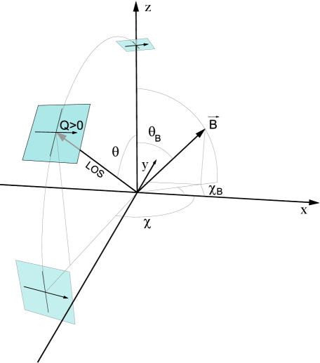
Figure 2.1: Reference system (x,y,z) used to place the generic line of sight (LOS) and magnetic field vector ($\vec{{\rm B}}$). The vertical axis is the solar radial direction passing through the point considered. From the observer point of view, the polarization is measured in the plane of the sky (coloured frames) containing the reference direction for $Q>0$.

We define the axis of reference assigned to a positive sign of Stokes Q as the direction in the plane of the sky that is parallel to the limb nearest to the scattering point (e.g., in Fig. 2.1, such direction is parallel to the x axis when $\chi=-\pi/2$). This also sets the same direction of reference for other quantities related to geometrical tensors: the radiation field components and the radiative transfer coefficients.

2.1.3 Line broadening mechanisms

Before presenting the expressions for the total radiative coefficients, we need to complete the description of the plasma element specifying the interaction mechanisms between the main atomic species and the surroundings. These interactions are affected by anisotropies, unresolved motions, quantum uncertainties, magnetic fields and by the radiation field illuminating the plasma. All together define the spectral variation of the absorption, emission and dispersion coefficients that characterize the radiative transfer properties of bound-bound transitions.

Since these properties are related to a complex refraction index, it is natural that the spectral variations of the radiative coefficients are characterized by a complex line profile $\Phi_{\nu}=\phi_{\nu}+i\psi_{\nu}$. The real part ($\phi_{\nu}$) describes the absorption and emission properties whereas the imaginary part ($\psi_{\nu}$) specify the dispersion effects in the polarization. They are probability distributions with unit area whose functions are given by the complex Voigt profile: $H+iL$. Next, we will consider the treatment of $\phi_{\nu}$ but the total dispersion profile follows from the same considerations with just substituting the real part of the Voigt profile H by the imaginary part L.

The spectral variation of the total absorption and emission coefficient $\phi(\nu)$ in a given spectral line is obtained by normalizing in area the Voigt function $H(a,x)$. In a weakly magnetized atmosphere with no macroscopic plasma velocities, the resulting profile is

$$\centering\phi(\nu-\nu_{0})\,=\,\frac{H(a,x)}{\sqrt{\pi}\Delta\nu_{D}},\@add@centering$$ (2.5)

with

$$\centering a\,=\,\frac{\gamma}{4\pi\Delta\nu_{D}},\@add@centering$$ (2.6)

$$\centering x\,=\,\frac{\nu-\nu_{0}}{\Delta\nu_{D}},\@add@centering$$ (2.7)

being $\gamma$ the total damping “constant”, $\Delta\nu_{D}$ the total Doppler width of the profiles and $\nu_{0}$ the line center frequency in the atom frame. The Voigt profile is the result of a convolution between a Lorentz profile characterizing the radiative plus collisional broadening mechanisms and the Gauss profile that describes the Doppler broadening. We have:

• Radiative broadening. The quantum uncertainty principle applied to the atomic energy levels limits the lifetime of the upper and lower levels of a transition. Thus, the infinitely sharp energy level is substituted by a statistical distribution function, the Lorentz profile, whose damping coefficient gives the radiative or natural broadening of the level $\gamma_{\rm rad}=1/\Delta t$ (with $\Delta t$ the mean lifetime of the level). In general, a number of radiative transitions involving a level $i$ set its total natural damping to

  $$\centering\gamma_{i}^{\rm{rad}}\,=\,\sum_{j<i}A_{ij}+\sum_{j>i}B_{ij}\bar{J}^{0}_{0}(\nu_{ij}),\@add@centering$$ (2.8)

  where the first sum accounts for the spontaneous emission rates and the second sum for the absorption ones, being $A_{ij}$ and $B_{ij}$ the corresponding Einstein coefficients and $J^{0}_{0}$ the angle-averaged mean intensity. The induced emission to lower levels can be similarly added (Mihalas, 1978). The total radiative broadening of the transition $\rm{u\rightarrow\ell}$ is then given by $\gamma^{\rm rad}=\gamma^{\rm rad}_{\ell}+\gamma^{\rm rad}_{u}$. We consider electric dipole radiative interactions, which connects atomic energy levels such that $\Delta J=0,\,\pm 1$ and $\Delta M=0,\,\pm 1$.

• Collisional or pressure broadening. This broadening appears when the main species emitting the spectral line radiation are perturbed by elastic collisions with other surrounding particles. The usual assumptions for modelling the collisional broadening in spectral lines are that the collisions are instantaneous (impact approximation), that they are isotropic and that the atomic emissions before and after the collisions are totally uncorrelated (Sobelman, 1973). In such case, the resulting spectral broadening is (again) a Lorentz profile whose damping $\gamma^{\rm col}$ can be simply added to $\gamma^{\rm rad}$ (by convolution of profiles), so giving the total $\gamma$ coefficient that enters in Eq. (2.6). Various collisional processes in turn contribute to $\gamma^{\rm col}$, being typically classified by the power index of the potential law that explains the collider interactions. Thus, we have the linear and quadratic Stark mechanisms ($\gamma^{\rm col}_{2}$ and $\gamma^{\rm col}_{4}$), resonance broadening ($\gamma^{\rm col}_{3}$) and Van der Waals broadening ($\gamma^{\rm col}_{6}$). Then,

  $$\centering\gamma=\gamma^{\rm rad}+\gamma^{\rm col}\,=\,\gamma^{\rm rad}+\sum_{i}\gamma^{\rm col}_{i}.\@add@centering$$ (2.9)

  Elastic collisions do not only broaden the profiles but also tend to eliminate the phase correlations (coherences) between energy substates $\ket{JM}$ and $\ket{JM^{\prime}}$, for what they are usually referred to as depolarizing collisions. Elastic collisions do not change the overall population of the level, but their actual rates are necessary to treat transitions between sublevels in the polarized case (Lamb & Ter Haar, 1971; Derouich & Sahal-Bréchot, 2003). On the contrary, inelastic collisions interchange energy between colliders, producing bound-bound transitions among different energy levels.

• Doppler broadening. Thermal motions below the plasma element scale produce spectral line broadening through the Doppler effect. The probabilistic distribution of velocities due to pure thermal motions is defined by the component form of a maxwellian distribution, which is a gaussian. The Maxwell distribution is strictly valid under LTE conditions, but it is commonly used in most astrophysical applications. The spectral variation of the pure thermal broadening as seen by an stationary observer is then obtained as a convolution of a delta $\delta(\nu^{\prime}-\nu)$ that describes radiation emitted by a single particle (being $\nu^{\prime}\approx\nu-v_{\rm LOS}\nu_{0}/c$ the Doppler-shifted frequency emitted by the particle) with the Maxwell distribution that characterizes the thermal motions of the emitting/absorbing atoms. On the other hand, it is usual to also assume here the presence of microturbulent motions when modeling the observed spectral line radiation using one-dimensional models of stellar atmospheres. The microturbulent broadening is given by non-thermal “turbulent” velocities ($v_{\rm micro}$) but are also assumed to have a random nature under the resolution element. The total spectral profile produced by both Doppler broadening mechanisms is other Gaussian whose total Doppler width is

  $$\centering\Delta\nu_{D}\,=\,\frac{\nu_{0}}{c}\sqrt{\frac{2kT}{m}+v^{2}_{\rm micro}},\@add@centering$$ (2.10)

  with $m$ the atomic mass of the main species. The microturbulent velocity $v_{\rm micro}$ is an ad-hoc fitting parameter that was introduced in the past to correct for deficiencies in plane-parallel modeling.

Other two “broadening” mechanisms affecting the spectral variation of the profiles are:

• Statistical redistribution in frequency. Thermal motions in the stellar atmosphere produce complete redistribution in frequencies (CRD) within the Doppler Gaussian core of the emerging line profiles. However, toward the line profile wings (lorentzian region), the probabilistic distribution of frequencies is instead controlled by the radiative and collisional elastic rates. If the former rates dominate ($\rm{\gamma^{rad}>\gamma^{col}}$) at some height, the electrons leave their atomic levels at exactly the same energy they arrived in, so maintaining the memory of the previous process (coherent scattering). But, as the elastic collisional rates increases downward in the atmosphere with the perturber density, they are able to produce a frequency reshuffling at those layers before radiative transitions occur. Thus, it approaches CRD in the spectral line wings. In intermediate layers where $\rm{\gamma^{rad}\approx\gamma^{col}}$, scattering is neither coherent nor completely redistributed, which is known as partial frequency redistribution or PRD. Both coherent scattering and complete redistribution can be equivalently treated, frequency by frequency, just correctly modelling the local processes that build the line profile. However, in PRD, the probability of scattering photons from one frequency to another is sensitive to the non-local monochromatic radiation field $J_{\nu}$ reaching each plasma element, which must be accounted for. In some cases, the lines affected by PRD exhibit extense line wings with challenging and complicated polarization patterns not fully understood so far. That is not the case of the IR triplet of the Ca ii lines, which are well described by CRD.

• Zeeman splitting. Considering a magnetically sensitive transition that connects an upper energy level $\rm{J_{u}}$ with a lower level $\rm{J_{\ell}}$, the presence of a magnetic field produces an energy splitting in the magnetic sublevels. This changes the spectral profiles. In general, the radiation emitted by the various transitions between the upper sublevels ${\rm M_{u}}$ and the lower ones ${\rm M_{\ell}}$ is usually referred to as Zeeman components. They are characterized by well- defined polarization properties that depend on the inclination $\hat{\theta}$ and azimuth $\hat{\chi}$ angles of the magnetic field vector measured in the reference frame of the ray with direction $\vec{\Omega}$. For the electric dipole mechanism, the only allowed transitions are those with $\rm{\Delta M=M_{u}-M_{\ell}=0}$ ($\pi$ components) and those with $\Delta M=\pm 1$ ($\sigma_{\rm b}$ and $\sigma_{\rm r}$ components, respectively). To specify the Zeeman profiles, we assume an isolated spectral line, no macroscopic velocity and a magnetic field weak enough for the Zeeman regime to hold. Furthermore, atomic polarization between magnetic sublevels is neglected in both levels of the transition. Then, the total line profiles are (e.g., Landi Degl’Innocenti & Landolfi, 2004)

  $$\phi_{I}(\nu,\vec{\Omega}) ={\displaystyle\frac{1}{2}\left[\phi_{0}\sin^{2}\hat{\theta}+\frac{\phi_{-1}+\phi_{1}}{2}\left(1+\cos^{2}\hat{\theta}\right)\right]},$$ (2.11a)

  $$\phi_{Q}(\nu,\vec{\Omega}) ={\displaystyle\frac{1}{2}\left[\phi_{0}-\frac{\phi_{-1}+\phi_{1}}{2}\right]\sin^{2}\hat{\theta}\cos 2\hat{\chi}},$$ (2.11b)

  $$\phi_{U}(\nu,\vec{\Omega}) ={\displaystyle\frac{1}{2}\left[\phi_{0}-\frac{\phi_{-1}+\phi_{1}}{2}\right]\sin^{2}\hat{\theta}\sin 2\hat{\chi}},$$ (2.11c)

  $$\phi_{V}(\nu,\vec{\Omega}) ={\displaystyle\frac{1}{2}\left[\phi_{1}-\phi_{-1}\right]\cos{\hat{\theta}}},$$ (2.11d)

  where

  $$\centering\phi_{q}=\sum_{M_{\ell}M_{u}}3\left(\begin{array}[]{ccc}J_{u}&J_{\ell}&1\\ -M_{u}&M_{\ell}&-q\end{array}\right)^{2}\phi(\nu-\nu_{J_{u}M_{u},J_{\ell}M_{\ell}})\qquad(q=-1,0,-1)\@add@centering$$ (2.12)

  describe the superposition of Zeeman components. Each $\phi(\nu-\nu_{J_{u}M_{u},J_{\ell}M_{\ell}})$ is a profile like Eq. (2.5) evaluated around its corresponding Zeeman frequency

  $$\centering\nu_{J_{u}M_{u},J_{\ell}M_{\ell}}=\nu_{0}+\nu_{L}(g_{u}M_{u}-g_{\ell}M_{\ell}),\@add@centering$$ (2.13)

  with $\nu_{0}$ the central wavelength of the transition and $\nu_{L}$ the Larmor frequency ($\nu_{L}[s^{-1}]=1.3996\,\times\,10^{6}\,B[G]$). In wavelength units, the Larmor frequency becomes the Zeeman splitting $\Delta\lambda_{B}=\lambda^{2}_{0}\nu_{L}/c$. When the Zeeman splitting is of the same order as the thermal Doppler width of the profiles, the polarization signals are in Zeeman regime. If the Zeeman splitting is small compared to the thermal width (e.g., due to weak magnetic fields or in some lines at optical wavelengths), the weak-field regime holds. In both cases the Zeeman components superpose producing a broadened line profile (magnetic broadening).

2.1.4 Radiative transfer coefficients

The coefficients appearing in Eq. (2.4) are the important connection between the micro and the macro state of the plasma. They have two contributions: continuum and line processes. In the solar atmosphere, the continuum opacities and emissivities are due to free-free and bound-free transitions, Thompson scattering and Rayleigh scattering.

On the other hand, the line terms are due to bound-bound transitions in the atomic species under consideration. Thus, line emission is described by the quantities $\epsilon^{l}_{I},\epsilon^{l}_{Q},\epsilon^{l}_{U}$ and $\epsilon^{l}_{V}$ in terms of the atomic density matrix elements and the emission profile $\phi_{\nu}$. Namely, in the case of weak magnetic field and no stimulated emission, the line emissions in I, U and Q for a transition $u\rightarrow{\ell}$ are (Manso Sainz & Trujillo Bueno, 2010):

$$\epsilon^{l}_{I}(\nu,\vec{\Omega})=\,\epsilon^{0}\rho^{0}_{0}+\epsilon^{0}\omega^{(2)}_{J_{u}J_{\ell}}\sqrt{3} \Big{\{}\frac{1}{2\sqrt{6}}\Big{(}3\mu^{2}-1\Big{)}\rho^{2}_{0}-\mu\sqrt{1-\mu^{2}}\Big{(}\cos{\chi}{\rm Re}[\rho^{2}_{1}]-\sin{\chi}{\rm Im}[\rho^{2}_{1}]\Big{)}$$

$$+\frac{1}{2}\Big{(}1-\mu^{2}\Big{)}\Big{(}\cos{2\chi}{\rm Re}[\rho^{2}_{2}]-\sin{2\chi}{\rm Im}[\rho^{2}_{2}]\Big{)}\Big{\}},$$ (2.14a)

$$\epsilon^{l}_{Q}(\nu,\vec{\Omega})=\,-\epsilon^{0}\omega^{(2)}_{J_{u}J_{\ell}}\sqrt{3} \Big{\{}\frac{3}{2\sqrt{6}}\Big{(}\mu^{2}-1\Big{)}\rho^{2}_{0}-\mu\sqrt{1-\mu^{2}}\Big{(}\cos{\chi}{\rm Re}[\rho^{2}_{1}]-\sin{\chi}{\rm Im}[\rho^{2}_{1}]\Big{)}$$

$$-\frac{1}{2}\Big{(}1+\mu^{2}\Big{)}\Big{(}\cos{2\chi}{\rm Re}[\rho^{2}_{2}]-\sin{2\chi}{\rm Im}[\rho^{2}_{2}]\Big{)}\Big{\}},$$ (2.14b)

$$\epsilon^{l}_{U}(\nu,\vec{\Omega})=\,-\epsilon^{0}\omega^{(2)}_{J_{u}J_{\ell}}\sqrt{3} \Big{\{}\sqrt{1-\mu^{2}}\Big{(}\sin{\chi}{\rm Re}[\rho^{2}_{1}]+\cos{\chi}{\rm Im}[\rho^{2}_{1}]\Big{)}$$

$$+\mu\Big{(}\sin{2\chi}{\rm Re}[\rho^{2}_{2}]+\cos{2\chi}{\rm Im}[\rho^{2}_{2}]\Big{)}\Big{\}},$$ (2.14c)

being $\mathrm{\mu=\cos(\theta)}$ and $\{\theta,\chi\}$ the inclination and azimuth of the ray $\vec{\Omega}$ with respect to the local solar vertical (quantization axis). The direction of reference for $Q>0$ is parallel to the nearest solar limb from the observed point. All the density-matrix components in these expressions correspond to the upper level of the transition. The $\omega^{(2)}_{J_{u}J_{\ell}}$ coefficients were introduced by Landi Degl’Innocenti (1984) and $\epsilon^{0}=(h\nu/4\pi)A_{u{\ell}}n_{\rm at}\sqrt{2J_{u}+1}\rho^{0}_{0}(J_{u})\phi_{\nu}$ is calculated with the Voigt profile $\phi_{\nu}$ and with $n_{\rm at}$ the total number of atoms of the considered species per unit volume.

Since in this thesis we assume a negligible contribution of atomic polarization to Stokes V, the corresponding line emission coefficient is dominated by the Zeeman effect. Thus, under the same previous assumptions:

$$\centering\epsilon^{l}_{V}(\nu,\vec{\Omega})=\epsilon^{0}\phi_{V}(\nu,\vec{\Omega}),\@add@centering$$ (2.15)

where $\phi_{V}$ was defined in Eq. (2.11d). We remark again that the angles ($\hat{\theta},\,\hat{\chi}$) appearing in such equation are measured with respect to the magnetic field direction. The corresponding absorption coefficients $\eta^{l}_{I},\eta^{l}_{Q},\eta^{l}_{U},\eta^{l}_{V}$ have identical expressions to the emission ones, but changing $A_{u{\ell}}\leftrightarrows B_{{\ell}u}$ and $u\leftrightarrows{\ell}$ in all the subscripts (including the ones in the expression of $\epsilon^{0}$). Furthermore, the $\rho^{K}_{Q}$ elements become the ones of the lower level of the transition.

The anomalous dispersion coefficients $\rho_{Q},\rho_{U},\rho_{V}$ are given by the same equations than the $\eta^{l}_{Q},\eta^{l}_{U},\eta^{l}_{V}$, respectively, but substituting the profiles $\phi_{\nu}$ (appearing in $\epsilon^{0}$ and in the Zeeman components of Eq. (2.12)) by the normalized anomalous dispersion profile $\psi_{\nu}$, introduced in Sec. 2.1.3. Considering the total complex profile $\Phi_{\nu}$ (Sec. 2.1.3), the absorption and dispersion coefficients can be seen as real and imaginary part of the same complex coefficient $X_{k}=\eta_{k}+i\rho_{k}$ with $k\equiv Q,\,U,\,V$.

The source function $S_{\nu}=\epsilon_{I}/\eta_{I}$ is an important quantity related to the intensity coefficients that describes the propagation of the intensity in the plasma. Under LTE conditions, it equals the Planck function.

2.1.5 Statistical equilibrium equations

In the case of LTE, the populations of the atomic energy levels are given by the Saha-Boltzmann distributions (Mihalas, 1978). They are totally determined by the local conditions of the plasma (basically, the density and a common temperature for all the particles) resulting in magnetic energy sublevels that are equally populated (hence, without atomic level polarization). When the spectral line is formed under NLTE conditions, the energy level and sublevel populations are not dominated by the collisional rates but by the radiative transitions. The radiation field interacts with matter through radiative excitations, photoionizations and their inverse processes (radiative desexcitations and recombinations), which strongly affects the atomic level populations especially in the outer atmosphere. To determine the resulting excitation state of the atoms in the plasma element, we have to solve the rate equations for the atomic density matrix corresponding to each level $i$. There is a rate equation per multipolar component of the density matrix. The rate equations account for the time evolution of the atomic system by specifying all the processes (see Fig. 2.2) that produce trasitions between energy states. In the case of a multilevel atom without hyperfine structure, and neglecting coherence between sublevels of different levels, the rate of change of the density matrix element $\rho^{K}_{Q}(J_{i})$ in the solar vertical frame reads (Landi Degl’Innocenti & Landolfi, 2004):

$$\begin{split}\frac{\rm d}{{\rm d}t}\rho^{K}_{Q}(J_{i})=-i\omega_{L}g_{J_{i}}\sum_{Q^{\prime}}K^{K}_{QQ^{\prime}}&\cdot\rho^{K}_{Q^{\prime}}(J_{i})-D^{(K)}(J_{i})\cdot\rho^{K}_{Q}(J_{i})\\ +\sum_{J_{u}}\sum_{K_{u}Q_{u}}\rho^{K_{u}}_{Q_{u}}(J_{u})\cdot T_{E}(J_{u};K_{u}Q_{u}\rightarrow J_{i};K&Q)+\sum_{J_{l}}\sum_{K_{l}Q_{l}}\rho^{K_{l}}_{Q_{l}}(J_{l})\cdot T_{A}(J_{l};K_{l}Q_{l}\rightarrow J_{i};KQ)\\ +\sum_{J_{u}}\sum_{K_{u}Q_{u}}\rho^{K_{u}}_{Q_{u}}(J_{u})\cdot T_{S}(&J_{u};K_{u}Q_{u}\rightarrow J_{i};KQ)\\ +\sum_{J_{u}}\sqrt{\frac{2J_{u}+1}{2J_{i}+1}}\rho^{K}_{Q}(J_{u})\cdot C^{(K)}_{S}(J_{u}\rightarrow&J_{i})+\sum_{J_{l}}\sqrt{\frac{2J_{l}+1}{2J_{i}+1}}\rho^{K}_{Q}(J_{l})\cdot C^{(K)}_{I}(J_{l}\rightarrow J_{i})\\ -\sum_{K^{\prime}Q^{\prime}}\rho^{K^{\prime}}_{Q^{\prime}}(J_{i})\cdot R_{E}(J_{i};KQ,K^{\prime}Q^{\prime}\rightarrow&J_{l})-\sum_{K^{\prime}Q^{\prime}}\rho^{K^{\prime}}_{Q^{\prime}}(J_{i})\cdot R_{A}(J_{i};KQ,K^{\prime}Q^{\prime}\rightarrow J_{u})\\ -\sum_{K^{\prime}Q^{\prime}}\rho^{K^{\prime}}_{Q^{\prime}}(J_{i})\cdot R_{S}&(J_{i};KQ,K^{\prime}Q^{\prime}\rightarrow J_{l})\\ -\rho^{K}_{Q}(J_{i})\cdot\bigg{[}\sum_{J_{u}}C^{(0)}_{I}(J_{i}&\rightarrow J_{u})+\sum_{J_{l}}{C^{(0)}_{S}}(J_{i}\rightarrow J_{l})\bigg{]},\end{split}$$ (2.16)

where we have included the effect of elastic and inelastic collisions assuming they are isotropic and that the impact approximation is valid. The first term in the r.h.s. of this equation accounts for the effect of the magnetic field (Hanle effect, see Sec. 2.4). The second term shows the action of the depolarizing collisions through the elastic collisional rate $D^{(K)}$. Both terms affect only the population imbalances inside the same energy level, either by the coherence or by population redistributions between energy sublevels.

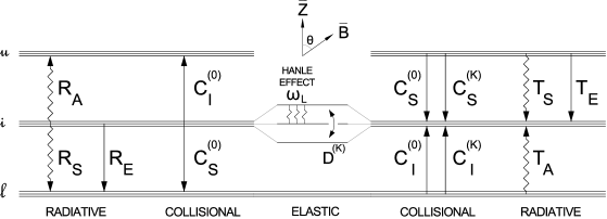
Figure 2.2: Schematic representation of the radiative, collisional and magnetic processes included in the rate equations of a given level $i$. All the upper and lower levels are represented by $u$ and ${\ell}$. On the right, the processes populating $i$ (transfer rates). On the left, the processes depopulating $i$ (relaxation rates). In the middle, the processes that do not change the overall population of $i$.

In general, the rate $X(J;KQ\rightarrow J^{\prime};K^{\prime}Q^{\prime})$ represents the probality that a transition carries atomic coherence from the level $J$, where is described by the multipole $\rho^{K}_{Q}$, to the level $J^{\prime}$, where it generates $\rho^{K^{\prime}}_{Q^{\prime}}$. The quantities $C_{I}$ and $C_{S}$ are the inelastic and superelastic collisional rates, respectively. The radiative rates are divided in the (populating) transfer rates $T_{A}$, $T_{E}$, $T_{S}$, and the (depopulating) relaxation rates $R_{A}$, $R_{E}$, $R_{S}$, which together describe the effects of absorption (A), spontaneous emission (E) and stimulated emission (S). The explicit expressions of all the rates can be found in Chapter 7 of Landi Degl’Innocenti & Landolfi (2004).

The whole system of $\rm{N_{KQ}}$ equations (one per unknown $\rho^{K}_{Q}$) at a given position in the atmosphere can be written in matrix form as:

$$\centering{\bf A}({\bm{\rho}})\cdot{\bm{\rho}}={\bf f},\@add@centering$$ (2.17)

where ${\bf A}$ is a $\rm{N_{KQ}\times N_{KQ}}$ matrix containing all the transition rates, ${\bm{\rho}}$ is a vector of length $\rm{N_{KQ}}$ containing the $\rho^{K}_{Q}$ elements for all the levels in the atomic model and $\bf{f}$ is a vector with zeros everywhere (assuming statistical equilibrium; i.e., $\frac{\rm d}{\rm dt}\rho^{K}_{Q}(J_{i})=0$). Note that ${\bf A}$ implicitly depends on the unknown $\rho^{K}_{Q}$ elements through the radiation field and that such a system of equations is highly non-linear.

The resulting set of equations is not linearly independent. To close the system, we have to substitute one of the equations, typically that of the ground level, by the equation of conservation of particles (the trace equation in the density matrix formalism). It establishes that the overall population of the atomic model considered is conserved:

$$\centering\sum_{i}\sqrt{2J_{i}+1}\rho^{0}_{0}(J_{i})=1\@add@centering$$ (2.18)

Thus, one of the zeros in $\mathbf{f}$ must be substituted by $1$.

The combination of the SEEs with the RTE poses the radiative transfer problem. The input of the former (the radiation field tensor components) depends on the output of the latter (the Stokes vector) and viceversa, which implies that an iterative method is needed to find the solution. Once the self-consistent solution for the $\rho^{K}_{Q}(J)$ elements is found, we can compute the emergent Stokes profiles for any desired line of sight.

2.1.6 Radiation field.

In concordance to the previous treatment of the density matrix, the radiation field illuminating each plasma element is also expressed in the spherical tensor representation. Thus, we obtain the tensor components $J^{K}_{Q}$, having $-K\leq Q\leq K$ with only three possible ranks $K=0,1,2$ (Landi Degl’Innocenti & Landolfi, 2004). They are integrals over frequency and angle of the Stokes vector components $I$, $Q$, $U$ and $V$. In particular, the even $K$ components are the main excitation sources for the scattering polarization. The explicit expressions for $K=0$ and $K=2$ are

$$\centering{\bar{J}^{0}_{0}}(z)=\displaystyle{\int{\rm d}{\nu}\oint\frac{{\rm d}\vec{\Omega}}{4\pi}\phi_{\nu}{{I_{\nu\vec{\Omega}}}}},\@add@centering$$ (2.19)

$$\centering{{\bar{J}^{2}_{0}}}(z)=\displaystyle{\int{\rm d}{\nu}\oint\frac{{\rm d}\vec{\Omega}}{4\pi}\phi_{\nu}\frac{1}{2\sqrt{2}}\left[(3\mu^{2}-1){{I_{\nu\vec{\Omega}}}}+3(1-\mu^{2}){Q_{\nu\vec{\Omega}}}\right]},\@add@centering$$ (2.20)

$$\centering{{\bar{J}^{2}_{1}}}(z)=\displaystyle{\int{\rm d}{\nu}\oint\frac{{\rm d}\vec{\Omega}}{4\pi}\phi_{\nu}\frac{\sqrt{3}}{2}{e}^{i\chi}\sqrt{1-\mu^{2}}\big{[}-\mu({I_{\nu\vec{\Omega}}}-{Q_{\nu\vec{\Omega}}})+iU_{\nu\vec{\Omega}}\big{]}},\@add@centering$$ (2.21)

$$\centering{{\bar{J}^{2}_{2}}}(z)=\displaystyle{\int{\rm d}{\nu}\oint\frac{{\rm d}\vec{\Omega}}{4\pi}\phi_{\nu}\frac{\sqrt{3}}{2}{e}^{i2\chi}\ \big{[}\frac{1}{2}({1-\mu^{2}}){I_{\nu\vec{\Omega}}}+\frac{1}{2}({1+\mu^{2}}){Q_{\nu\vec{\Omega}}}+i\mu U_{\nu\vec{\Omega}}\big{]}}.\@add@centering$$ (2.22)

As usually along this thesis, the reference direction for $Q>0$ (defined in the plane of the sky) is chosen parallel to the solar limb that is nearest to the local vertical (z axis). The anisotropy factor for each spectral line transition is defined as:

$$\centering w_{\mathrm{line}}(z)={\sqrt{2}}\frac{\bar{J}^{2}_{0}(z)}{\bar{J}^{0}_{0}(z)}.\@add@centering$$ (2.23)

It ranges from $w_{\mathrm{line}}=-0.5$ (azimuthally independent incident radiation field contained in the horizontal plane) to $w_{\mathrm{line}}=1$ (collimated vertical beam), vanishing at the bottom of the atmosphere where the radiation field is unpolarized and isotropic. The dominating factor $(3\mu^{2}-1)I$ in the definition of $\bar{J}^{2}_{0}$ makes that the rays with $54.73\,\mbox{${}^{\circ}$}<\theta<125.27\,\mbox{${}^{\circ}$}$ (which are mainly horizontal) contribute always negatively to the anisotropy factor, while radiation coming from other directions (that is, mainly vertical) always contributes positively. The anisotropy factor is thus especially sensitive to temperature gradients (Trujillo Bueno, 2001; Landi Degl’Innocenti & Landolfi, 2004).

The $J^{2}_{Q}$ components with $Q\neq 0$ measure the breaking of the axial symmetry of the radiation field. In plane-parallel atmospheres only the magnetic field can break the symmetry of the radiation field and generates such components.

2.2 Numerical methods for polarized radiative transfer.

2.2.1 Integration of the transfer equation.

The formal solver used in our calculations is based on a short-characteristics scheme (Kunasz & Auer, 1988), which allows the numerical integration of the RT equations along ray paths between neighbouring points.

The RTE (see Eqs. (2.4)) in compact form can be written as

$$\centering\frac{\rm{d}}{\rm{ds}}{\bf I}={\bm{\epsilon}}-{\bf KI},\@add@centering$$ (2.24)

where s is the geometrical distance along the ray and ${\bf K}$, ${\bm{\epsilon}}$ and ${\bf I}$ are the propagation matrix, the emission and the Stokes vectors, respectively. Making a change of variable to $\tau=\int\eta_{I}{\rm d}s$ and formally integrating between consecutive points along the ray under consideration we get (Rees et al., 1989):

$$\centering{\bf I}_{\rm O}={\bf I}_{\rm M}\,{\rm e}^{-\Delta\tau}+\int^{\tau_{\rm M}}_{\tau_{\rm O}}\left[\frac{1}{\eta_{I}}{\bm{\epsilon}}-\left(\frac{1}{\eta_{I}}{\bf K}-{\bf 1}\right){\bm{I}}\right]{\rm e}^{-(\tau-\tau_{\rm O})}{\rm d}\tau,\@add@centering$$ (2.25)

where ${\bf 1}$ is the $4\times 4$ identity matrix, $\Delta\tau$ is the optical thickness between M and O and $\tau$ is the optical path along the ray.

For a given direction and frequency, the optical depth discretization is obtained from the geometrical depth grid, taking into acount its definition and assuming an exponential dependence of $\eta_{I}$ with z. If we assume a parabolic variation of $\mathbf{S}={\bm{\epsilon}}/\eta_{I}$ between three successive points M, O and P along the ray, while assuming that $({\bf K}/\eta_{I}-1){\bf I}$ varies linearly between M and O, then we can perform the integral in Eq. (2.25) and obtain the Stokes vector at point O with (Trujillo Bueno, 2003c)

$$\centering[\mathbf{1}+\Psi^{\prime}_{\rm O}\,\mathbf{K}^{\prime}_{\rm O}]\mathbf{I}_{\rm O}=\,[{\rm e}^{-\Delta\tau_{\rm M}}\mathbf{1}+\Psi^{\prime}_{\rm M}\,\mathbf{K}^{\prime}_{\rm M}]\,\mathbf{I}_{\rm M}+\Psi_{\rm M}\,\mathbf{S}_{\rm M}+\Psi_{\rm O}\,\mathbf{S}_{\rm O}+\Psi_{\rm P},\,\mathbf{S}_{\rm P},\@add@centering$$ (2.26)

where $\Psi_{M,O,P}$ are numerical coefficients that depend on the optical distances $\Delta\tau_{\rm M}$ between M and O, and $\Delta\tau_{\rm P}$ between O and P. Similarly, $\Psi^{\prime}_{\rm M,O}$ only depend on $\Delta\tau_{\rm M}$. Explicit expressions for these coefficients are given in Kunasz & Auer (1988). This generalization of the short-characteristics method to the polarized case is called DELOPAR. To apply it, we start at one atmosphere’s boundary and successively calculate $\mathbf{I}_{\rm O}$ at each grid point, proceeding along any given ray direction until the opposite boundary.

Finally, to obtain the radiation field tensors (see Section 2.1.6) we have to integrate numerically the calculated Stokes parameters for all the points in the frequency and angular discretization. For the frequency quadrature we use a trapezoidal rule over the absorption profiles. For the polar angles we use a Gaussian quadrature in inclination and an equally spaced trapezoidal rule for the azimuth. Formally, we can write the radiation field tensor components as

$$\centering\mathbf{J^{K}_{Q}}=\mathbf{\Lambda}[{\bm{\rho}}^{\bf K}_{\bf Q}]+{\bf T^{K}_{Q}},\@add@centering$$ (2.27)

where $\mathbf{\Lambda}$ is an operator giving the response of the radiation field to perturbations in the density-matrix elements and the $\bf{T^{K}_{Q}}$ vector gives the contribution of the boundary conditions to the radiation field at the spatial points considered.

2.2.2 Statement of the iterative problem.

In general, to solve the RT problem with polarization it is necessary to calculate the self-consistent values for the $\rho^{K}_{Q}$ multipolar components of the density matrix at each spatial point $i$ in the model. The main problem is that such components are coupled in a highly non-linear and non-local way through the radiation field. The strategy is to start from an estimation of the solution and to perform iterative corrections to that estimation until arriving to self-consistent values.

The procedure is as follows. Given an initial guess $\rho^{K\,\rm{old}}_{Q}(i)$ at each depth, the radiative transfer equations are integrated to obtain the Stokes parameters (at each depth and for any angle and frequency), which gives the radiation field tensor components $J^{K\,\rm{old}}_{Q}(i)$ at each of the $\mathrm{N_{z}}$ heights of the model atmosphere under consideration. From Eq. (2.27), it can be expressed as

$$\centering\mathbf{J^{K\,\rm{old}}_{Q}}=\mathbf{\Lambda}[{\bm{\rho}}^{{\bf K}\,\rm{old}}_{\bf Q}]+{\bf T^{K}_{Q}},\@add@centering$$ (2.28)

Once the $J^{K\,\rm{old}}_{Q}(i)$ are estimated, the transfer rates can be calculated and the algebraic system formed by the SEEs (Eq. 2.17) is linearized and solved as

$$\centering{\bf A}^{\rm old}\cdot{\bm{\rho}}^{\rm new}={\bf f}\@add@centering$$ (2.29)

to obtain the new corrected elements $\bm{\rho}^{\rm{new}}={\bm{\rho}^{\rm{old}}}+\delta{\bm{\rho}}$. We remark that $\bf{A^{\rm old}}$ depends on the ${\bm{\rho}^{\rm{old}}}$ values.

If the initial guess is not the exact solution, then $\delta{\bm{\rho}}\neq 0$ and Eq. (2.29) will have a certain residual error. The objective is to find the $\bm{\rho}^{\rm{new}}$ values (equivalently, the corrections $\delta{\bm{\rho}}$) that leads to precisely fulfill Eq. (2.17). The linearization makes the solution at each step to never be exact, but successive iterations reduce the errors to the desired small size as $\delta{\bm{\rho}}\rightarrow 0$ (Hubeny & Lanz, 1992).

The different iterative methods applied to the RT problem are distinguished by the way they approximate in Eq. (2.29) the $\bm{\rho}^{\rm{new}}$ values from the $\bm{\rho}^{\rm{old}}$ by modifying $\bf{A^{\rm old}}$. The simplest method is the $\Lambda$-iteration, which consists in introducing the $\bm{\rho}^{\rm{old}}$ values again into Eq. (2.28) to build $\bf{A^{\rm old}}$, thus using only the $\rho^{K}_{Q}$ values of the previous iterative step. The convergence rate of this method is very poor in optically thick atmospheres because the numerical information is propagated through the spatial grid along one photon mean free path per iteration, which takes many iterations to radiatively connect all the points in the atmosphere.

In the following, we specify the conceptual strategies used by more sophisticated methods to estimate the new $\rho^{K}_{Q}$ values. Basically, we require a formal solver to integrate the RT equations and a suitable linearization of the SEE that guarantees convergence in the iterative process.

2.2.3 Iterative scheme.

The linearization of Eqs. (2.17) can be achieved by several methods. The one we use in our calculations is based on two techniques: operator splitting (Cannon, 1973) and preconditioning (Rybicki & Hummer, 1991; Socas-Navarro & Trujillo Bueno, 1997).

Applied to the polarized case, the operator splitting strategy rewrites the formal solution of the RT equation given by Eq. (2.27) as:

$$\centering\mathbf{J^{K}_{Q}}=\mathbf{\Lambda}^{\bf*}[{\bm{\rho}}^{{\bf K}}_{\bf Q}]+(\mathbf{\Lambda}-\mathbf{\Lambda}^{\bf*})[{\bm{\rho}}^{{\bf K}}_{\bf Q}]+{\bf T^{K}_{Q}},\@add@centering$$ (2.30)

where $\mathbf{\Lambda}^{\bf*}$ is an approximation to the full operator $\mathbf{\Lambda}$. This splitting will allow the substitution of some $\rho^{K\,{\rm old}}_{Q}$ values by their implicit “new” values in the equations, which approaches the final solution at a higher convergence rate. A good choice for the approximate operator $\Lambda^{*}$ is the diagonal of the full $\Lambda$ operator (so making it local) because it is easy to obtain and to invert. This is the extension of the Accelerated $\Lambda$-iteration (ALI) method to the polarized case (Trujillo Bueno & Fabiani Bendicho, 1995).

The next step is to approximate the dominant tensor component $J^{0}_{0}(i)$ by considering that, for each i-th spatial point, it can be obtained using the $\rho^{K\,{\rm old}}_{Q}$ values at all grid points but only $\rho^{0\,{\rm new}}_{0}(i)$ at point i. From Eq. (2.30), this can be expressed as

$$\centering J^{0}_{0}(i)=J^{0\,{\rm old}}_{0}(i)+\Lambda(i,i)[\rho^{0}_{0}(i)^{\rm{new}}-\rho^{0}_{0}(i)^{\rm{old}}],\@add@centering$$ (2.31)

where the numerical values of the r.h.s. are known except for $\rho^{0}_{0}(i)^{\rm{new}}$, which is the implicit unknown to be calculated in the current iterative step. Here, the $\rho^{0}_{0}$ values correspond to the upper level of the transition.

Substitution of Eq. (2.31) into the SEE yields a non-linear system of algebraic equations. This non-linearity is due to terms of the form $\rho^{K}_{Q}({\ell})J^{0}_{0}$ that are tied to the absorption rates pumping population and coherence from each lower level $\ell$. In order to linearize such terms we calculate them at each spatial point $i$ making (Trujillo Bueno, 2003c)

$$\centering\rho^{K}_{Q}(J_{\ell})J^{0}_{0}\rightarrow\rho^{K}_{Q}(J_{\ell})^{\rm{new}}J^{0\,{\rm old}}_{0}+\Lambda(i,i)[\rho^{K}_{Q}(J_{\ell})^{\rm old}\rho^{0}_{0}(J_{u})^{\rm{new}}-\rho^{K}_{Q}(J_{\ell})^{\rm new}\rho^{0}_{0}(J_{u})^{\rm{old}}],\@add@centering$$ (2.32)

again with all the quantities evaluated at point $i$, the $\rho^{0}_{0}$ components corresponding to the upper level of the transition and $\rho^{K}_{Q}$ to the lower one. This is the preconditioning scheme we use in our calculations. It allows to transform the statistical equilibrium equations given by Eqs. (2.17) in a linear system at each iterative step.

In summary, the combination of preconditioning and operator splitting achieves linearity building ${\bf A^{\rm old}}$ with a strategical combination of “new” and “old” terms indicated by Eq. (2.32). With respect to $\Lambda$ iteration, the only extra calculation in the ALI method are the local elements $\Lambda(i,i)$, which can be efortlessly obtained using a formal solver based on short-characteristics.

2.2.4 Evaluation of $\Lambda^{*}$

We can detail Eq. (2.27) as

$$0\rightarrow \quad\mathbf{J^{0}_{0}}=\mathbf{\Lambda}_{00}[{\bm{\rho}}^{\bf 0}_{\bf 0}(u)]+\mathbf{\Lambda}_{01}[{\bm{\rho}}^{\bf 2}_{\bf 0}(u)]+\cdots+\mathbf{\Lambda}_{\rm 0N}[{\bf\hat{{\bm{\rho}}}}^{\bf 2}_{\bf 2}(u)]+{\bf T}^{0}_{0}$$ (2.33a)

$$1\rightarrow \quad\mathbf{J^{2}_{0}}=\mathbf{\Lambda}_{10}[{\bm{\rho}}^{\bf 0}_{\bf 0}(u)]+\mathbf{\Lambda}_{11}[{\bm{\rho}}^{\bf 2}_{\bf 0}(u)]+\cdots+\mathbf{\Lambda}_{\rm 1N}[{\bf\hat{{\bm{\rho}}}}^{\bf 2}_{\bf 2}(u)]+{\bf T}^{2}_{0}$$ (2.33b)

$$\beta\rightarrow \quad\vdots$$

$$N\rightarrow \quad\mathbf{\hat{J}^{2}_{2}}=\mathbf{\Lambda}_{\rm N0}[{\bm{\rho}}^{\bf 0}_{\bf 0}(u)]+\mathbf{\Lambda}_{\rm N1}[{\bm{\rho}}^{\bf 2}_{\bf 0}(u)]+\cdots+\mathbf{\Lambda}_{\rm NN}[{\bf\hat{{\bm{\rho}}}}^{\bf 2}_{\bf 2}(u)]+{\bf\hat{T}}^{2}_{2}$$ (2.33c)

where ${\bf J^{K}_{Q}}$, ${\bf T^{K}_{Q}}$ and ${\bm{\rho}}^{\bf K}_{\bf Q}$ are formal vectors with $N_{z}$ components, one per spatial grid point, whose imaginary parts are indicated with the hat ( $\hat{}$ ); and where $N+1$ is the total number of multipole components different from zero in the problem considered (6 in our most general case). Each $\Lambda_{\alpha\beta}$ are $N_{z}\times N_{z}$ operators with elements $\Lambda_{\alpha\beta}(i,j)$. Their expressions in terms of $\Psi$, $\Psi^{\prime}$ and $\rho^{K}_{Q}(\ell)$ multipoles are given in Manso Sainz (2002).

In the standard methods, only the calculation of a few $\Lambda_{\alpha\beta}(i,j)$ elements is necessary. We show the Eqs. (2.33) just to illustrate how the calculation of the required operator elements can be done at the same time the formal solution of the Stokes vector is computed. Namely, to obtain an specific $\Lambda_{\alpha\beta}(i,j)$ element, we have to calculate the $j$-th component of the ${\bf J^{K}_{Q}}$ multipole in the equation $\beta$ after making ${\bf T^{K}_{Q}}=0$ and taking equal to zero all the ${\bm{\rho}^{K}_{Q}}$ vectors except for the $i$-th component of the ${\bm{\rho}}^{\bf K}_{\bf Q}$ multipole corresponding to the $\alpha$ position, which has value unity. The result is that the $\Lambda_{\alpha\beta}(i,j)$ values can be obtained at the same time and following similar operations than when calculating the radiation field tensors with the formal solution.

To understand how the different iterative methods work, we can also make explicit the action of a given $\Lambda_{\alpha\beta}$ operator. Take for instance $\Lambda_{00}$. In general, that component operates as

$${\displaystyle J^{0}_{0}(i)}=\Lambda_{00}(i,1)[\rho^{0}_{0}(1)]^{\rm A}+ \cdots+\Lambda_{00}(i,i-1)[\rho^{0}_{0}(i-1)]^{\rm A}$$ (2.34a)

$$+\Lambda_{00}(i,i) [\rho^{0}_{0}(i)]^{\rm B}$$ (2.34b)

$$+\Lambda_{00}(i,i+1)[\rho^{0}_{0}(i+1)]^{\rm C} +\cdots+\Lambda_{00}(i,N_{z})[\rho^{0}_{0}(N_{z})]^{\rm C}$$ (2.34c)

$$+ T^{K}_{Q},$$ (2.34d)

where all the letters in brackets especify a spatial position and the superscripts A,B and C can be “old” or “new” depending on the iterative scheme followed. Thus, in the simplest case of $\Lambda$-iteration they are $A=B=C=\rm{old}$, which means that $J^{K}_{Q}=J^{K\,{\rm old}}_{Q}$ for any K and Q. This can be interpreted as if we were solving the SEE with a radiation field that does not react to the corrections in the populations because the operator ${\bf A}$ of Eqs. (2.17) was exclusively built with the old population estimation. In the ALI method used in this thesis, $A=C=$old but $B={\rm new}$, which means that $J^{0}_{0}$ is only affected by the local corrections in the new populations. In the case we choose $A=B=\rm{new}$ with $C={\rm old}$, we would be updating the contributions given by all the spatial points that were previously considered when performing the formal solution of the RT equation along a ray. In other words, we use an approximate triangular operator ${\bm{\Lambda}^{*}}$ that contains more information about the radiative couplings between points in the atmosphere than the diagonal approximate ${\bm{\Lambda}^{*}}$ operator. This gives a faster iterative method known as Gauss-Seidel and SOR, which can be also efficiently solved (Trujillo Bueno & Fabiani Bendicho, 1995). The main drawback of these operator splitting methods is the deterioration of the convergence rate when the spatial resolution of the grid is refined. In the limit of an infinitely fine grid, all such methods will converge as slow as the $\Lambda$-iteration method. For iterative methods whose convergence rate is insensitive to the grid size consult Fabiani Bendicho et al. (1997).

2.3 Line formation in moving atmospheres

The existence of systematic velocity fields in solar and stellar atmospheres is well-documented by abundant observational evidence. Plasma motions appear to be present on all scales, from microscopic thermal to macroscopic motions (i.e., nonthermal velocities that are coherent over distances much larger than a particle mean-free path). Indeed, the consideration of systematic motions is essential to explain the observations in many astrophysical contexts: pulsating stars, hot stars with fast stellar winds, expanding nebulae, supernovae and fast changes in solar prominences are good examples. In particular, the increasing interest in the highly inhomogeneous and dynamic solar chromosphere has served to highlight plasma dynamics as a key point to understand the outer solar layers.

The modelling of radiative transfer in dynamic atmospheres is more complicated than in static atmospheres. On one hand, the presence of velocity gradients makes the opacity and emissivity angle-dependent, which may have a significant impact on the radiation field anisotropy. On the other hand, any of the existing methods to solve the RTE add higher levels of complexity in dynamic atmospheres, with significant increase of the computational demand, either because the RTE adopts a more involved form to treat the problem in a comoving frame, or due to a meaningful increment in the numerical resolution (Mihalas, 1978). Such drawbacks are more severe when including the polarization.

Most of the theoretical works done so far have only considered polarized light in static atmospheres, being however unbalanced by the large number of observational investigations studying it in dynamic media. On top of that, most of the computational tools and theoretical investigations in moving atmospheres only consider the effect of the velocities in the framework of the Zeeman line-formation theory (e.g., Stenflo, 1994; Socas-Navarro et al., 2000; Uitenbroek, 2011), sometimes even without putting an special emphasis on the analysis of dynamic effects. Other authors treat the problem in very schematic situations (Molodij & Bommier, 2011; Landolfi & Landi Degl’Innocenti, 1996). With respect to the scattering polarization, the work of Nagendra (1996) accounts for the impact of macroscopic velocities in moving media using the two-level atom approximation for describing resonance lines.

2.3.1 Effect of the velocity on the radiative transfer.

Although in many physical situations the RTE can be formulated as in the static regime, in many others a full dynamic treatment is required. For instance, the influence of bulk motions is small for the continuum, but can be important in spectral lines because even small Doppler shifts can cause large changes in opacity (leading to significant variations in the radiation received by a stationary observer). In general, the effects acting on the emitted line radiation due to systematic velocities in a stellar atmosphere are: Doppler shifts, producing variations of the line profiles with frequency; aberration of photons, producing variations of the line profiles with the ray direction; and advection, producing variations of the line profiles with the distance along the line of sight.

The numerical methods required for solving the general line-formation problem in moving media are reviewed in Mihalas & Kunasz (1986). Nowadays, the discussion is still around techniques and valid approximations that can be applied in different situations to solve the RTE for the intensity. In a nutshell, there are four essential ways of treating radiative transfer in atmospheres with velocity gradients: (i) Monte Carlo methods (Bernes, 1979; Lucy, 2005); (ii) Sobolev or supersonic approximations (Sobolev, 1958, 1960); (iii) observers’ frame methods; and, (iv) comoving frame methods (Mihalas, 1978). The first method is not suitable for treating optically thick atmospheres . The relatively low solar velocity fields, with outflows not much larger than the microturbulent velocities (in comparison with extreme events), also excludes the Sobolev approximation.

The preference between the observer’s and the comoving frame methods in points (iii) and (iv) will depend on various issues. For instance, the application of the comoving frame method has the advantage that the opacity and emissivity coefficients are not affected by motion and may be treated as in the static case (i.e., since they are isotropic for the static case, then they are isotropic also in a local reference frame in a moving atmosphere). Other important point is that the comoving frame method admits the simplification of using angle-averaged redistribution functions in calculations where PRD is required. However, the RTE becomes more complicated due to an additional term containing the frequency derivative of the intensity. Lorentz transformations have also to be considered to transmit the information between different comoving frames. Finally, the comoving-frame transfer equation is usually solved using Feautrier variables, which furthermore limits the applicability of this method to monotonic velocity fields. Very recently, we have been aware of improved (and more sophisticated) methods to solve the RTE in the comoving frame that allow the treatment of arbitrary velocity fields (Baron et al., 2012), but they do not represent a significant advantage with respect to the computational effort of doing it in the observer’s frame.

Thus, although the solution of the RTE in the comoving frame would require much less angle-quadrature points when macroscopic velocities are present (Mihalas, 1978), we treat the radiative transfer in the observer’s frame because it is better suited to the non-monotonic velocities that are present in the chromosphere. Other authors have used this strategy for solving the problem under the Zeeman line-formation theory in the absence of atomic polarization (e.g., Stenflo, 1994; Uitenbroek, 2002). In the observer’s frame, the opacity and emissivity of the material, as seen by a stationary observer, become angle-dependent but the formal structure of the RTE is maintained. Consequently, it is also a suitable method for including the effect of the macroscopic velocity in a previously existing code, as it has been the case in this thesis. The details of the implementation are left for the next chapters.

• Frequency redistribution in dynamic cases:

An issue that will trascend our results is how they could be affected by PRD effects in dynamic situations. The investigation of PRD in the polarization is presently limited by the applicability of the theoretical framework developed so far. The quantum theory of spectral line polarization (Landi Degl’Innocenti & Landolfi, 2004) that we follow in our investigation is based on the hypothesis that the pumping radiation field has no spectral structure across intervals smaller than the frequency separation between interfering atomic levels (flat-spectrum approximation), which is equivalent to the CRD approximation. Despite its limitations, this theory represents the most robust quantum approach to the physics of polarization developed so far and it even has demonstrated to be useful in situations out of their applicability regime.

In absence of macroscopic motions, CRD is a good approximation for weak lines whose extreme wings do not require extensive line transfer. On the contrary, the modelling of very strong (typically resonant) lines should be done in principle using PRD. For CRD to be valid across the whole line profile, the intrinsic radiative rates (most importantly $A_{u{\ell}}$) must be low enough, in such a way that collisional rates overcome them in middle layers. On the contrary, if the radiative transition probabilities are very large (as in resonant lines), collisional damping will no longer be an efficient frequency mixer already from deeper layers, leaving an intermediate extended region in which PRD holds. Even in that case, the intensity profiles of solar resonant lines (e.g., Mg ii or Ca ii H and K) calculated with PRD and with CRD have almost identical absorption cores. In typically subordinated lines whose lower atomic energy levels are not connected to the fundamental levels (e.g., the Ca ii IR triplet lines), CRD can be safety applied in static media (Uitenbroek, 1989).

On the other hand, for flow speeds on the order of the mean thermal speed, velocity gradients could cause the line center intensity to depend more strongly on frequency and direction than in comparable static media because they tend to assymetrize the Maxwell distributions describing the thermal motions at the core. Hence, the CRD assumption would deteriorate (Hummer & Rybicki, 1968). On the basis of previous works, we expect the difference between PRD and CRD profiles of resonant lines to be enhanced as the ratio of systematic to turbulent velocities decreases and as the line formation region is larger, showing an effectively thick chromosphere (Drake & Linsky, 1983). In next chapters, we deal with atmospheres whose maximum velocities ($\sim 0-25\,\rm{km\,s^{-1}}$) are comparable to the mean turbulent velocity ($\sim 3\,\rm{km\,s^{-1}}$). However, we are interested in the polarization amplitudes of non-resonant lines at their cores, where the PRD effects should be notably less limitating. Indeed, the exact line profile at the wings is not relevant to our aims because their physics is actually very different from the physics of the core, which is the true recorder of the Hanle and Zeeman effects and where the observational Caii IR triplet signals show a measurable polarization.

2.3.2 Effect of the velocity in the SEE.

Being a conservation law applied to a volume element, the statistical equilibrium equations depend on the plasma velocities. For instance, the $\rm{\rho^{0}_{0}}$ component of each atomic level J satisfy a rate equation of the form

$$\centering\frac{\partial\rho^{0}_{0}(J)}{\partial t}+\nabla\left[\vec{v}\rho^{0}_{0}(J)\right]=\,\mathcal{P}(J\rightarrow J^{\prime})-\mathcal{P}^{\prime}(J\rightarrow J^{\prime})\@add@centering$$ (2.35)

where the r.h.s contains the variations of $\rm{\rho^{0}_{0}}$ due to radiative and collisional transitions (both included in the generic processes $\mathcal{P}$ and $\mathcal{P}^{\prime}$) that populate $(J^{\prime}\rightarrow J)$ and depopulate $(J\rightarrow J^{\prime})$ the level $J$. In static cases, the l.h.s. is zero because statistical equilibrium is assumed. In dynamic but non-relativistic calculations, the atmosphere can still be considered stationary ($\partial/\partial t=0$) and the advection term is usually neglected.

The advection term accounts for the amount of material that enters or exits the fluid element volume considered. The rate at which the non-relativistic material can enter or leave the volume element in the simulation is assumed slow compared with that at which the atomic system reaches the statistical equilibrium (which is a fast microscopic process following the atomic transition rates). The conclusion is that statistical equilibrium can be safety applied.

2.3.3 Effect of the velocity on the atomic density matrix.

Due to the Doppler effect, the radiation field experienced by an atom depends on its velocity $\vec{v}$. Consequently, the density matrix will also depend on it (Landi Degl’Innocenti & Landolfi, 2004). Being $\rho^{K}_{Q}(J;\vec{v})$ the spherical statistical tensor of the atomic system dependent on $\vec{v}$, and $f(\vec{v})$ the velocity distribution function of the atoms in a given point of the atmosphere, a complete statistical description of the atomic collectivity is given by the product $f(\vec{v})\rho^{K}_{Q}(J;\vec{v})$. Such quantity is the so-called velocity-space density matrix.

This formalism is presently being developed for the case of a two-level atom with infinitely-sharp levels and it has shown to be equivalent to the redistribution matrix formalism for treating PRD effects (Belluzzi et al., 2013). Indeed, it constitutes a more general approach to such a problem because it is able to account for the phenomenon of pure Doppler redistribution including broadening collisions and lower level polarization in multilevel systems. Consequently, the velocity-space density matrix formalism seems to be also a likely solution for describing the macroscopic velocity effects in PRD-affected lines.

2.4 The Hanle Effect in the solar atmosphere

2.4.1 Description

The Hanle effect can be understood classically (Hanle, 1924) with the oscillator model for the atomic electrons. In this picture, the magnetic field makes the oscillating electrons to precess around the magnetic field direction, producing a rosette pattern (Fig. 2.3, left drawing). There is a competition between the radiative damping rate of such oscillator and the rate of Larmor precession, which is proportional to the magnetic field strength (Stenflo, 1994; Trujillo Bueno, 2001; Landi Degl’Innocenti & Landolfi, 2004). Thus, when the former prevails, the Hanle effect can leave its fingerprint on the Stokes parameters (Fig. 2.3, right drawing). From the point of view of the observer, the action of the Hanle effect is a modification of the linear polarization, measured by Stokes Q and U. When the Zeeman splitting is negligible compared with the line width, the transverse Zeeman effect signals (affecting Q and U) are of second order, in such a way that Q and U only measure the scattering polarization and its modification by the Hanle effect.

Figure 2.3: Rosette pattern describing the motion of an undamped charged oscillator in a magnetic field (left) and the pattern obtained when taking radiative decay into account (right).

In the following, we introduce how the orientation and strength of a magnetic field in a solar plasma element produces the Hanle effect in the quantum theory. Consider a spectral line whose upper and/or lower levels can be polarized ($\mathrm{J_{\ell,u}>1/2}$). Then, the Hanle effect consists in the modification of such atomic polarization through a magnetic field whose Larmor frequency ($\mathrm{\omega_{L}=8.79\times 10^{6}B}$) is comparable to the inverse of the radiative lifetime of the energy levels of the transition. This defines one critical magnetic field strength $B_{H}$ per polarized level, given in gauss by

$$\centering 8.79\times 10^{6}\,g_{L}\,B_{H}\sim 1/\mathrm{t_{life}},\@add@centering$$ (2.36)

where $\mathrm{g_{L}}$ is the Landé factor and $\mathrm{t_{life}}$ (in seconds) can be approximated with $\mathrm{1/A_{u\ell}}$ for the upper level and with $\mathrm{1/(B_{\ell u}J^{0}_{0})}$ for the lower one. As the Larmor frequency in wavelength units is the Zeeman splitting, Eq. (2.36) is equivalent to say that the Hanle effect operates when the Zeeman splitting is comparable to the natural width of the energy levels. Note that the Zeeman effect produces clear polarization signals when the Zeeman splitting is comparable to the thermal width of the line profiles.

The above considerations suggest that the Hanle effect can be seen as a result of the coupling between the magnetic field with Larmor frequency and the radiative rates. In the quantum approach, this coupling alters the quantum coherence between pairs of magnetic sublevels and modifies the atomic level polarization. The direct action of the magnetic field on the density-matrix multipoles is introduced in the rate Eqs. (2.16) through the magnetic term, which also accounts for the geometry of the physical situation. Geometry is a essential piece of the Hanle effect. The Hanle magnetic term is (Landi Degl’Innocenti & Landolfi, 2004)

$$\centering-i\omega_{L}g_{L}\sum_{Q^{\prime}}\mathcal{K}^{K}_{QQ^{\prime}}\rho^{K}_{Q^{\prime}}(J).\@add@centering$$ (2.37)

Choosing the quantization axis along the vertical, the only non-zero magnetic kernels for $K=0,1,2$ can be expressed as

$$\mathcal{K}^{K}_{QQ} =\,\displaystyle Q\,\cos{\theta_{B}}\qquad (\Delta Q=0),$$ (2.38a)

$$\mathcal{K}^{K}_{QQ^{\prime}} =\,\displaystyle\sqrt{\frac{2K-1-|Q\cdot Q^{\prime}|/K}{2}}\cdot\sin{\theta_{B}}\cdot e^{\mathrm{i}(Q^{\prime}-Q)\chi_{B}}\qquad (\Delta Q=\pm 1),$$ (2.38b)

where the angles define the orientation (inclination $\theta_{B}$ and azimuth $\chi_{B}$) of the magnetic field in the reference frame of the solar vertical passing through the scattering point. Eqs. (2.37) and (2.38) indicate that the magnetic field can create or destroy coherences with a certain $Q\neq 0$ by changing and dephasing any multipolar component with $Q^{\prime}=Q\pm 1$, but it cannot modify the overall population of a level by itself. Similarly, those equations indicate that population imbalances $\rho^{K}_{0}$ can be created from coherence terms with $Q=\pm 1$. This way, the magnetic field transfers the information about its orientation and strength to the quantum system. The Hanle effect becomes important when the orientation of the magnetic field produces a significative symmetry breaking in the atmosphere ($\theta_{B}\rightarrow 90\,\mbox{${}^{\circ}$}$) and when the field strength is near the critical values for the energy levels (Hanle regime). In other cases, coherences vanish and the magnetic kernel in the SEE cancels out.

2.4.2 A hands-on guide to the Hanle equations

Next, we underline the physics of the Hanle effect and give some technical details and approximations to work with it.

Figure 2.4: Reference system (x,y,z) used to place the generic line of sight ($\vec{\Omega}$) and magnetic field direction ($\vec{{\rm B}}$). The vertical axis is the radial direction of the Sun through the point being considered. The reference direction set by the observer in the plane of the sky are given by the unit vectors ${\rm\vec{e}_{a}}$ and ${\rm\vec{e}_{b}}$. The positive Stokes-Q direction is defined in that plane by $\gamma$. The magnetic field reference frame is similar to the one in $\vec{\Omega}$, but placed along $\vec{\rm B}$ and having $\gamma_{\rm B}=0$ for simplicity.

Eddington-Barbier approximation

We start estimating the linear polarization at line center (Trujillo Bueno, 2003a). We consider a strong spectral line not affected by stimulated emission and emerging from a plane-parallel atmosphere that is assumed to be well described by the Eddington-Barbier approximation. Then, its fractional linear polarization X$/$I (with X$=$Q or X$=$U) is given by:

$$\centering\frac{X}{I}\simeq\,\frac{\epsilon^{l}_{X}}{\epsilon^{l}_{I}}-\frac{\eta^{l}_{X}}{\eta^{l}_{I}},\@add@centering$$ (2.39)

where all the terms in the r.h.s. have to be evaluated at $\mathrm{\tau^{LOS}=1}$. Afterwards, this approximate formula will give us some useful expressions.

No Zeeman-splitting case

In the Hanle regime, the Zeeman splitting is small in comparison with the spectral line width, so the absorption and emission profiles do not depend on the magnetic quantum numbers [$\mathrm{\phi=\phi(\nu-\nu_{u{\ell}})=\phi(J_{u},J_{\ell})}$]. Then, Eq. (7.16e) of Landi Degl’Innocenti & Landolfi (2004) can be written as :

$$\centering\epsilon_{i}(\nu,\vec{\Omega})=\,\frac{h\nu}{4\pi}N\sum_{\alpha_{\ell}J_{\ell}}\sum_{\alpha_{u}J_{u}}\sqrt{2J_{u}+1}A_{u{\ell}}\sum_{KQ}\omega^{(K)}_{J_{u}J_{\ell}}\mathcal{T}^{K}_{Q}(i,\vec{\Omega})\rho^{K}_{Q}(J_{u})\phi(\nu-\nu_{u{\ell}}).\@add@centering$$ (2.40)

Hereafter, we will refer to the emission vector components and propagation matrix elements as $\mathrm{\epsilon_{i}}$ and $\mathrm{\eta_{i}}$, being $\mathrm{i=0,1,2}$ for Stokes I, Q and U. Similar expressions for the absorption coefficients $\mathrm{\eta_{i}(\nu,\vec{\Omega})}$ are obtained from the previous equation with the changes $\mathrm{A}_{u{\ell}}\leftrightarrows B_{{\ell}u}$, $J_{u}\leftrightarrows J_{\ell}$ and $\mathrm{\omega}^{(K)}_{J_{u}J_{\ell}}\leftrightarrows\omega^{(K)}_{J_{\ell}J_{u}}\cdot(-1)^{K}$. In Eq. (2.40), the tensor $\mathcal{T}^{K}_{Q}$ gives the geometrical transformation that projects the multipolar components $\rho^{K}_{Q}$ from the quantization axis to the LOS reference system, thus expliciting the polarized emission of the media along the considered ray. We always have to choose a quantization axis for the angular momentum (typically the local solar vertical or the magnetic field direction). It has associated the reference system in which $\mathcal{T}^{K}_{Q}$ and $\rho^{K}_{Q}$ are defined. Besides that, the previously assumed independence of the spectral profiles on the magnetic quantum numbers makes the emissivity and absorption coefficients invariant under rotations of the reference frame. It means that in Eq. (2.40) we can express $\mathcal{T}^{K}_{Q}$ and $\mathrm{\rho^{K}_{Q}}$ in any system (the same for both). Apart from this, we must also choose the observer reference system by setting the LOS ($\vec{\Omega}$) and the angle $\gamma=\gamma_{\Omega}$ that defines the direction for positive Q (see Fig. 2.4).

Non-blended spectral line

If the spectral lines of the atomic system do not overlap, there is only one transition involved at line center (summations in $\alpha J$ disappear from Eq. 2.40). Then, making the substitution $\epsilon^{0}=\frac{h\nu}{4\pi}N\sqrt{2J_{u}+1}A_{u{\ell}}\phi(0)$, we get:

$$\centering\epsilon^{l}_{i}(\vec{\Omega})=\,\epsilon^{0}\sum_{KQ}\omega^{(K)}_{J_{u}J_{\ell}}\left[\mathcal{T}^{K}_{Q}(i,\vec{\Omega})\right]^{\vec{z}}\left[\rho^{K}_{Q}(J_{u})\right]^{\vec{z}},\@add@centering$$ (2.41)

where the superscript on the square brackets indicates that we are evaluating those quantities in the reference frame of the local vertical. The advantage of setting the quantization axis along the vertical is that the angles of the geometrical tensors are referred to a common and invariant direction, which facilitates the calculation of the radiation field components ($\bar{J}^{K}_{Q}$) independently on the magnetic field direction (the magnetic field can be differently oriented from point to point). Eq. (2.41) is the simplest general expression for the Hanle effect that allows us to derive other published in literature. It shows clearly that the emission of polarized light in the Hanle regime is directly proportional to the atomic density matrix elements projected to our line of sight by the tensor $\mathcal{T}^{K}_{Q}$. If the illumination at the atmosphere boundaries is not polarized and there are no sources of atomic orientation, the components with odd $K$ are zero in the summation. However, an important point is that the mere existence of a limb darkening at every point of the solar atmosphere generates atomic alignment and terms with even K that contribute to the emisivity in Q and U. Such $\rho^{K}_{Q}$ elements are tipically modified by the magnetic kernel in the SEE, following Eq. (2.37). That is the essence of the Hanle effect on the scattering polarization.

To explicit the dependence of the polarized emission on the coherences we recall Equations (2.14). They are derived from Eq. (2.41) with $i=0,1,2$, $K=0,2$ and $-K<Q<K$ , after choosing a reference direction for $Q>0$ that is parallel to the limb nearest to the scattering point (that is, with $\gamma=\pi/2$). The setting of a reference direction simplify the geometrical tensors (from Table 5.6 in Landi Degl’Innocenti & Landolfi, 2004). For instance, the emissivity in Stokes U:

$$\epsilon^{l}_{2}(\vec{\Omega}) =\,-\epsilon^{0}\omega^{(2)}_{J_{u}J_{\ell}}\sqrt{3}\{\sqrt{1-\mu^{2}}(\sin{\chi}{\rm Re}[\rho^{2}_{1}]+\cos{\chi}{\rm Im}[\rho^{2}_{1}])$$

$$\qquad\qquad\qquad+\mu(\sin{2\chi}{\rm Re}[\rho^{2}_{2}]+\cos{2\chi}{\rm Im}[\rho^{2}_{2}])\},$$ (2.42)

with $\chi$ and $\theta=\cos^{-1}(\mu)$ the azimuth and inclination of the LOS in the reference frame of the local vertical. In particular, the emission in U vanishes when coherences are zero. However, Stokes Q also depends on the non-vanishing $\rho^{2}_{0}$ components excited by the radiation field anisotropy.

The explicit angular dependence set by the tensors $\mathcal{T}^{K}_{Q}$ always measures rotations from the reference frame in the quantization axis ($\vec{\mathrm{z}}$ or $\vec{\mathrm{B}}$, usually) to the one in the LOS (see Fig. 2.4). On the other hand, any spherical tensor can be expressed along a different quantization axis by following the corresponding rotation law. Namely, we can pose the $\rho^{K}_{Q}$ elements in the $\vec{\mathrm{z}}$ system as a combination of the ones in the $\vec{\mathrm{B}}$ system with:

$$\centering[\rho^{K}_{Q}(J)]^{\vec{{\rm z}}}=\sum_{Q^{\prime}}[\rho^{K}_{Q^{\prime}}(J)]^{\vec{{\rm B}}}\mathcal{D}^{K}_{Q^{\prime}Q}(R)^{*},\@add@centering$$ (2.43)

where the matrices $\mathcal{D}^{K}_{Q^{\prime}Q}$ carry out the rotations given by the Euler angles $R=(\alpha\beta\gamma)$ going from the magnetic field to the solar vertical reference frame. The advantage of applying this relation in order to express a given equation as a function of the $\rho^{K}_{Q}$ elements of the magnetic field frame is that they simplify in certain circumstances (see below).

Hanle effect in the saturation regime

In saturation, the magnetic field strength is very intense in comparison with the critical Hanle field of the atomic levels ($B>>B_{H}$). Thus, the separation in energy between them destroy all coherences in the magnetic field reference frame ($[\rho^{K}_{Q}]^{SAT}=\rho^{K}_{Q}\cdot\delta_{Q0}$). In this case, the polarization of the emergent spectral line radiation does not depend on the field strength but only on its orientation, which still plays an active role in the radiative transfer through the radiative coefficients. The emission (and similarly the absorption) coefficients can then be particularized from Eqs. (2.14) (or Eq. (2.41)) by conveniently expressing the components $\rho^{K}_{Q}$ as in Eq.(2.43). Following it, we write the rotation going from the $\vec{\mathrm{B}}$ to the $\vec{\mathrm{z}}$ frame as $R_{1}=(0,-\theta_{B},-\chi_{B})$. Recalling the saturation assumption, the coherence terms vanish in the $\vec{\mathrm{B}}$ frame and the only relevant transformations are thus given by $[\rho^{2}_{Q}]^{\vec{\mathrm{z}}}=[\rho^{2}_{0}]^{\vec{\mathrm{B}}}\mathcal{D}^{K}_{0Q}(R_{1})^{*}$, where:

$$\mathcal{D}^{2}_{00}(R_{1})^{*} =\frac{1}{2}(3\cos^{2}{\theta_{B}}-1)$$ (2.44)

$$\mathcal{D}^{2}_{01}(R_{1})^{*} =\sqrt{\frac{3}{2}}\sin{\theta_{B}}\cos{\theta_{B}}{\rm e^{i\chi_{B}}}$$

$$\mathcal{D}^{2}_{02}(R_{1})^{*} =-\sqrt{\frac{3}{8}}\sin^{2}{\theta_{B}}{\rm e^{-i\chi_{B}}}.$$

Substituting the so given $\rho^{2}_{Q}$ in Eq. (2.42) we obtain:

$$\epsilon^{l}_{2}(\vec{\Omega}) \propto\,-\Big{[}\sqrt{1-\mu^{2}}\sin{(\chi-\chi_{B})}\sin{(2\theta_{B})}+\mu\sin{[2(\chi-\chi_{B})]}\sin^{2}{\theta_{B}}\Big{]}\cdot[\rho^{2}_{0}]^{\vec{\mathrm{B}}},$$ (2.45)

where the alignment in the magnetic case can be related to the alignment in the non-magnetic case as

$$[\rho^{2}_{0}]^{\vec{\mathrm{B}}}= \,\frac{1}{2}(3\cos^{2}{\theta_{B}}-1)\cdot[\rho^{2}_{0}]^{\mathrm{B=0}},$$ (2.46)

Following similar steps for the emission and absorption terms in $i=0,1,2$, we can evaluate the Eq. (2.39) for Q$/$I and U$/$I. In the weak-anisotropy regime ($\rho^{2}_{0}<<\rho^{0}_{0}$) holding in stellar atmospheres we can finally write:

$$\frac{Q}{I}\simeq \,\frac{3}{8\sqrt{2}}\Big{[}(1-\mu^{2})(3\cos^{2}{\theta_{B}}-1)-2\mu\sqrt{1-\mu^{2}}\sin{(2\theta_{B})}\cos{(\chi_{B}-\chi)}$$

$$+(1+\mu^{2})\sin^{2}{\theta_{B}}\cos{[2(\chi_{B}-\chi)]}\Big{]}\cdot(3\cos^{2}{\theta_{B}}-1)\cdot\mathcal{F}$$ (2.47a)

$$\frac{U}{I}\simeq \,-\frac{3}{4\sqrt{2}}\Big{[}\sqrt{1-\mu^{2}}\sin{(2\theta_{B})}\sin{(\chi_{B}-\chi)}$$

$$-\mu\sin^{2}{\theta_{B}}\sin{[2(\chi_{B}-\chi)]}\Big{]}\cdot(3\cos^{2}{\theta_{B}}-1)\mathcal{F},$$ (2.47b)

where $\mathcal{F}=\omega^{(2)}_{J_{u}J_{\ell}}\sigma^{2}_{0}(J_{u})-\omega^{(2)}_{J_{\ell}J_{u}}\sigma^{2}_{0}(J_{\ell})$ is the non-magnetic contribution of the fractional atomic alignment ($\sigma^{2}_{0}=\rho^{2}_{0}/\rho^{0}_{0}$) generated in the levels of the transition. The evaluation of Eqs. (2.47) for different configurations of magnetic field and LOS is an interesting exercise that shows the behavior of the scattering polarization in every case.

Particularizing to the configuration in which the LOS and the magnetic field vector are contained in perpendicular planes ($\chi_{B}-\chi=\pi/2$), we obtain the Eqs (3) and (4) of Trujillo Bueno (2010). If, instead, we particularize to the forward scattering case ($\mu=1$) with arbitrary magnetic field direction, we obtain:

$$\frac{Q}{I} \simeq\,\frac{3}{4\sqrt{2}}\cdot\sin^{2}{\theta_{B}}\cdot(3\cos^{2}{\theta_{B}}-1)\cos{[2(\chi_{B}-\chi)]}\cdot\mathcal{F}$$ (2.48a)

$$\frac{U}{I} \simeq\,\frac{3}{4\sqrt{2}}\cdot\sin^{2}{\theta_{B}}\cdot(3\cos^{2}{\theta_{B}}-1)\sin{[2(\chi_{B}-\chi)]}\cdot\mathcal{F},$$ (2.48b)

Remind that all the terms in these approximated expressions have to be evaluated at $\mathrm{\tau^{LOS}=1}$. Apart from the effect of the limb-darkening induced anisotropy on the linear polarization (contained in $\mathcal{F}$), Eqs. (2.48) isolate other geometric effects in the polarization of the saturated Hanle effect. Note that in forward scattering both Stokes parameters are basically equivalent in their geometrical dependence, having the same maximum and minimum values. Furthermore, a vertical magnetic field makes zero the forward scattering Stokes parameters because nothing breaks the axial symmetry around the LOS when considering a plane-parallel atmosphere.

Being in forward scattering, we also particularize Eqs. (2.48) to have $\chi_{B}-\chi=\pi/2$, which is equivalent to align the positive-Q direction along the projection of the magnetic field onto the plane of the sky (because $\gamma$ was set to $\pi/2$). Then, we obtain

$$\frac{Q}{I} \simeq\,-\frac{3}{4\sqrt{2}}\sin^{2}{\theta_{B}}\cdot(3\cos^{2}{\theta_{B}}-1)\cdot\mathcal{F},$$ (2.49)

with $U=0$. On the other hand, dividing Eqs. (2.48) between them, we arrive to

$$\frac{U}{Q} =\,\tan{[2(\chi_{B}-\chi)]}.$$ (2.50)

If we set the positive Stokes Q along the x axis (see Fig. 2.4), then $\chi=-\pi/2$. In this configuration, the azimuth of the magnetic field defines the direction of maximum polarization for the emerging light beam (such maximum is given by Eq. (2.49)). We will take advantage of this fact in Chapter 6.

Zero-field regime

Finally, in the zero-field regime and for any line of sight, the result would be simpler. Repeating all the procedure, we obtain:

$$\frac{Q}{I} \simeq\,\frac{3}{2\sqrt{2}}(1-\mu^{2})\mathcal{F},$$ (2.51)

with $U=0$, and always with $\mu=\cos{\theta}$ and the positive-Q reference being parallel to the limb nearest to the scattering point. Here, the polarization is zero in forward scattering and maximum when looking at the solar limb.

Note that in any situation the anisotropy of the radiation field is always affecting the microscopic system in the plasma element through the factor $\mathcal{F}$. However, the expression of such atomic polarization into a measurable radiative quantity depends on the observer point of view. Hereafter, in all the subsequent chapters, the quantization axis for the angular momentum will be along the local solar vertical.

2.4.3 Hanle effect at work: two examples.

The cases in which the Hanle effect is commonly employed to measure solar magnetic fields are illustrated here in two particular geometries:

• Observation near the solar limb (typically $\mu=0.1$). Here, the non-magnetic signals are given by Stokes Q due to pure scattering (i.e., to the atomic polarization caused by the anisotropy of the radiation field). If a magnetic field is present, the Hanle effect produces depolarization. To measure the magnetic field we need to know the theoretical non-magnetic polarization amplitudes as a reference. We could also calibrate theoretically the relative response that similar lines have to the magnetic field and use the calibration for real measures (line-ratio technique). In the case of the Ca ii IR triplet lines that can be observed at the solar limb (Fig. 2.5), we expect that the relative polarization amplitudes observed are due to a depolarizing magnetic field. This case will be treated in chapter 5.

  

  Figure 2.5: Recordings (November 17, 1994 ) of the spectral regions around the three IR lines of Ca ii made with ZIMPOL near the solar north pole limb by Stenflo et al. (2000). The level of the continuum polarization is represented by the horizontal dashed lines.

• Forward scattering at disk center ($\mu=1$). In this case, the non-magnetic signals are zero because the observer is looking along a symmetry axis (assuming a plane-parallel atmosphere). If the field is purely vertical nothing changes. If the field is inclined, Hanle-induced polarization appears. The more horizontal the magnetic field is, the larger the polarization. This case will be treated in detail in Chapter 6.

  

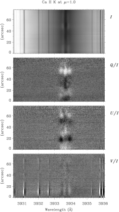
  Figure 2.6: Spectropolarimetric observation of the K-line of Caii at solar disk center in quiet regions. Obtained with ZIMPOL at the McMath Telescope in Kitt Peak Observatory by Stenflo (2006).

Chapter 3 Developed tools and methodology.

In this chapter, we describe some computer programs, procedures and techniques that we have developed to treat the radiative transfer (RT) of scattering polarization in dynamic solar models, including software that we have found very useful to analyze and understand the results of our investigations. The most important tools to mention are: the RT code that we have used to synthetize the scattering polarization in the presence of velocity gradients; an iterative computer procedure to suitably redistribute the nodes of the numerical spatial grid and achieve convergence of the RT problem in atmospheric models with strong height variations; a code to calculate response functions of the Stokes parameters; a code to perform Principal Component Analysis in measured and theoretical Stokes profiles; a Python-based software to interactively analyze the atmospheric models together with the resulting spectropolarimetric maps; and finally, a series of codes and plotting routines that use the Mayavi package to visualize and analyze 3D models of the solar atmosphere interactively.

3.1 A RT code for dynamic scattering polarization.

3.1.1 Traviata.

Traviata is a multilevel RT code for the synthesis of the spectral line polarization that is due to atomic polarization and the Hanle effect in weakly magnetized stellar atmospheres (Manso Sainz & Trujillo Bueno, 2003b). The relevant equations that it implements have been already described in Chapter 2. A very significant part of this thesis work is based on the improvements applied to Traviata. The following is a brief summary of the capabilities of the original program.

The physical assumptions in which the calculations were based are:

1. Plane-parallel geometry of arbitrary optical thickness.

2. Complete redistribution in frequency.

3. NLTE.

4. Atomic levels can be polarized. Populations imbalances and coherence between different magnetic energy sublevels of the same J level can exist. The magnetic sublevels of different J levels do not interfere (multilevel approximation).

5. Magnetic fields are weak enough for the splitting of the absorption profiles to be negligible (much lower than the thermal width of the spectral line).

6. Impact approximation for collisions.

7. Stimulated emission is neglected.

To solve the RT of the second kind, Traviata follows the following numerical approach (Manso Sainz, 2002; Manso Sainz & Trujillo Bueno, 2003b, 2010):

1. The equations are formulated within the spherical tensors representation of the density matrix and radiation field tensor. There are $\rm{(2J+1)(J+1)}$ unknowns $\rm{\rho^{K}_{Q}}$ with K even, for each level with integer angular momentum J , and $\rm{(2J+1)J}$ unknowns for each level with semi-integer angular momentum J .

2. The radiative transfer equations for the Stokes parameters are integrated along short characteristics using the quasi-parabolic DELO method (DELOPAR; see Section 2.2.1).

3. The iterative corrections for the unknowns (the statistical tensors $\rm{\rho^{K}_{Q}}$) are calculated applying a suitable generalization to the multilevel atom case of the Jacobian iterative method described in Trujillo Bueno & Manso Sainz (1999). This implies writing down the statistical equilibrium equations taking explicitly into account the contribution of the diagonal components of the $\Lambda$ operator and linearizing according to Eq.(2.32) and the procedure in Sec. 2.2.3.

4. The iterative scheme can be speeded up through polynomial Ng-acceleration Auer (1987).

When using semiempirical models of the solar atmosphere, the number density of the ion under consideration is first computed in NLTE. Having the overall population of the ion and after reading the model variables, Traviata computes the background continuum opacities. The first initialization is done calculating the population of the levels in LTE. In a second step, they are then used as a guess to obtain the population of the levels in the standard NLTE case without polarization. Afterwards, it solves the SEE at each point in the atmosphere for the multipolar components of the atomic density matrix plus the conservation of particles equation (Eq. (2.18)) to calculate the full excitation state of the atomic system. Next, it calculates the radiation field at each point in the model atmosphere for each allowed radiative transition in the model atom applying the formal integration of the radiative transfer equations for the Stokes parameters (DELOPAR method). The radiation field tensors $\rm{J^{K}_{Q}}$ are calculated and used to obtain the new excitation state of the atomic system and so on, iteratively, until reaching the final solution for the $\rho^{K}_{Q}$ values.

3.1.2 The new version of Traviata

We have extended Traviata to investigate the effect of macroscopic vertical velocities on the linear polarization produced by scattering processes in spectral lines, as well as on the circular polarization profiles caused by the Zeeman effect. Maintaining the previous characteristics of the code, we have implemented the following improvements:

1. Inclusion of the effect of vertical (non-relativistic) velocities in the RT.

   The RT problem considered by Traviata is posed and solved in the observer’s frame (see Sec. 2.3.1). In this strategy, there is a unique reference frame fixed in space and all the motions in the plasma are related to it. Thus, each plasma element receives an spectral illumination that depends on the inclination of the rays but also on the relative motion with respect to other plasma elements that shift the line profiles by the Doppler effect (more details in Chapter 4). In this case, the absorption, emission and dispersion line profiles depend on position, frequency, spectral transition and, additionally, on the inclination of the rays of the angular quadrature. It extends to associated quantities such as the absorption, emission and dispersion coefficients. The line profiles are calculated for each spatial point $i$ by shifting the static profiles (see Sec. 2.1.3) with the Doppler velocity $\mu_{k}V_{i}$, where $\mu_{k}=\cos(\theta_{k})$, $\theta_{k}$ is the inclination of the ray $k$ in the angular quadrature, and $V_{i}=(\nu_{0}v_{i}/c)/\Delta\nu_{Di}$ is the Doppler shift, in Doppler width units, produced by the vertical velocity $v_{i}$ at point $i$. For instance, the dynamic absorption profile would be $\phi^{\prime}=\phi({\rm x}-\mu_{k}{V_{i}})$ with ${\rm x}$ the Doppler frequency axis. Upward velocities gives blue shifts. For a given model stratification, the maximum effect of the velocity on the profiles occurs at the height where the Doppler velocity is $V_{\rm max}={\rm Max}[{\nu_{0}}\bm{v}/(c\bm{\Delta\nu_{D}})]$.

2. Redefinition of variables and numerical grids.

   • The frequency axis is common and fixed along the whole calculation. The frequency axis is symmetric with respect to line center and has now double extension in wavelength than in the static case in order to cover the asymmetries and Doppler shifts produced by motions in the profiles.

   • The extension of the frequency axis is larger enough for the line coefficients to have a smooth transition to the continuum even in the presence of large velocities. This avoids imprecisions in the normalization of the profiles to unit area.

   • The line core region is adaptively built with a resolution notably larger than in the wings to correctly sample the features of the emergent moving profiles. The wings resolution is smaller and quadratically decreasing towards the continuum. The minimum frequency resolution at the core must give 2 points per minimum Doppler width $\Delta\nu_{D}^{\rm min}$ in the atmosphere ($\Delta{\rm x}=1/2$, in minimum Doppler units). Furthermore, the cutoff frequency ${\rm x_{c}}$ setting the end of the core is dictated by the maximum expected Doppler shift $\delta{\rm x}^{\rm{max}}=\nu_{0}v^{\rm max}/(c\Delta\nu_{D}^{\rm min})$ (expressed here in minimum Doppler units). Then, the core width in Traviata is set to the most restrictive case:

     $${\rm x_{c}}=\delta\rm{x^{max}}+N^{0}_{c}$$ (3.1)

     where everything is in minimum Doppler units and $N^{0}_{c}$ is a safeguard constant taking into account an extra width due to the large profiles width at the hottest layers.

   • The angular and spatial numerical grids are heavily restricted by the presence of velocities and the maximum Doppler shift in the model stratification. If we want the spectral variation of the profiles to be well sampled, the change in Doppler velocity $\Delta(\mu_{k}V_{i})=\Delta\mu_{k}\cdot V_{i}+\Delta V_{i}\cdot\mu_{k}$ in our spatial and angular grid has to be small enough (i.e., of the order of half Doppler width) everywhere, not only between adjacent points along the same ray but also between adjacent points along the same height.

     On one hand, this sets a constraint for the angular grid that can be evaluated as:

     $$|\Delta\mu_{\rm max}V_{\rm max}|\lesssim\frac{1}{2},$$ (3.2)

     where $\Delta\mu_{\rm max}$ gives the maximum allowed angular step in the quadrature. On the other hand, the spatial grid is constrained by:

     $$\centering\Delta V_{i}=|V_{i}-V_{i-1}|\lesssim 1/2,\@add@centering$$ (3.3)

     which limits the maximum Doppler velocity gradient between two adjacent layers $i$ and $i-1$ in the atmosphere.

   • Once the iterative problem is solved for the atomic density-matrix elements, the emergent Stokes vector is calculated using a very fine frequency grid for capturing with precision all the spectral features. The maximum number of spectral grid points is limited to $191$ during the iteration and to $505$ in the last formal integration of the RT equation.

3. Inclusion of the variation of the magnetic field with height.

   In semiempirical models like FALC (Fontenla et al., 1993), there is no description of the magnetic field. Usually, in this case the magnetic field is added ad-hoc with constant parameters along the whole atmosphere. For Traviata to be able to compute realistic models showing variations of the magnetic field strength and orientation with height, we have also extended the variables to consider such variations.

4. Calculation of Stokes V in the Zeeman regime (optional choice).

   • Under the assumption of the weak field regime, Stokes V is due to the longitudinal Zeeman effect while Stokes Q and U are due to scattering and Hanle polarization, being the linear signals of the transverse Zeeman effect a second-order contribution. In such a case, the radiative transfer equations for Stokes Q and U decouple from the RT equation for Stokes V to a good level of approximation.

     Dynamic Traviata solves the iterative problem for the populations of the energy sublevels using the transfer equations in the scattering and Hanle regime. At the end, when the atomic density multipoles are solved, the total level populations are used to solve the Zeeman transfer equation independently for I and V along the observer LOS:

     $$\frac{\rm{d}}{\rm{ds}}\left(\begin{array}[]{c}I\\ V\end{array}\right)=\left(\begin{array}[]{c}\epsilon_{I}\\ \epsilon_{V}\end{array}\right)-\left(\begin{array}[]{cc}\eta_{I}&\eta_{V}\\ \eta_{V}&\eta_{I}\end{array}\right)\left(\begin{array}[]{c}I\\ V\end{array}\right).$$ (3.4)

     The dispersion or magneto-optical terms have been neglected in the calculation of Stokes V because their contributions to the circular polarization are insignificant in weakly magnetized atmospheres. To solve the system of equations we transform it in two independent equations:

     $$\frac{\rm{d}}{\rm{ds}}\left(\begin{array}[]{c}I^{+}\\ I^{-}\end{array}\right)=\left(\begin{array}[]{c}\epsilon^{+}\\ \epsilon^{-}\end{array}\right)-\left(\begin{array}[]{c}\eta^{+}I^{+}\\ \eta^{-}I^{-}\end{array}\right),$$ (3.5)

     creating the variables $I^{\pm}=I\pm V$, $\epsilon^{\pm}=\epsilon_{I}\pm\epsilon_{V}$ and $\eta^{\pm}=\eta_{I}\pm\eta_{V}$. Both equations are solved along the LOS using a parabolic short-characteristic method to get the emergent $I^{+}$ and $I^{-}$ profiles for each frequency and spectral transition. The solution for the original variables is then obtained with $I=(I^{+}+I^{-})/2$ and $V=(I^{+}-I^{-})/2$. There is a slight inconsistency in calculating again the intensity with Stokes V while neglecting Q and U, but it is justified by the uncoupling between linear and circular polarization in weak magnetic fields. The intensity profile resulting from the scattering problem is almost the same as the one obtained from the Stokes V calculation, being in most cases undistinguishable except for a negligible (magnetic) broadening in some Zeeman signals.

   • The Stokes V line radiative coefficients are calculated neglecting atomic orientation. This implies that they can be calculated at each point from Eqs. (2.14) and (2.15), where the spectral profiles for the Stokes V coefficients are given by Eq. (2.11d). We repeat it here for the sake of clarity:

     $$\centering\phi_{V}(\nu,\vec{\Omega})=\frac{1}{2}\left[\phi_{1}-\phi_{-1}\right]\cos{\hat{\theta}},\@add@centering$$ (3.6)

     with $\hat{\theta}$ the direct angle between the local magnetic field vector and the direction $\vec{\Omega}$ of the given emerging ray passing through the considered plasma element. Working in the reference frame of the solar vertical, this angle can be calculated locally at every point in the atmoshere with:

     $$\centering\cos{\hat{\theta}}=\cos{\theta}\cos{\theta_{B}}+\sin{\theta}\sin{\theta_{B}}\cos{(\chi_{B}-\chi)},\@add@centering$$ (3.7)

     with $\theta$ and $\chi$ the angles defining the LOS.

   • With these modifications Traviata gives the linear polarization signals produced by scattering polarization and Hanle effect, while additionally delivers the Stokes V profiles resulting from the Zeeman effect, always considering the velocity and the magnetic field gradients.

5. Automatization for working with a large number of models.

   The code is launched from an IDL program that provides all the initialization settings. This program is adapted to the particular model atmosphere under consideration. For the case of a 3D data cube, it is considerably sophisticated because a strategy for running each model column in a specific order and with an adaptative initialization of the density-matrix elements (see next point) is needed. The automatization also includes the management and listing of models with convergence problems that have to be recomputed with other interpolation grid, with other parameter settings or with other initializing populations. Finally, the automatization includes the compilation process (which is now more complex due to a re-modularization and re-organization of the subroutines) and the possibility of reading and representing the outputs with additional programs.

6. Initialization of the populations.

   The code has 4 execution modes. In the first mode the code reads a file with a given solution of the $\rho^{K}_{Q}$ elements and directly integrate the RTE to obtain the emergent Stokes vector for one LOS. In the second mode Traviata solves the full RT problem by initializing the iterative process with the overall populations given by the atmospheric model (when they are available). In the third mode, the code solves the problem initializing with the $\rho^{K}_{Q}$ elements that were previously obtained for an adjacent column in the model. This can save some time when running a dataset whose consecutive models in the series are similar. Finally, the fourth mode is the standard one in which the initialization is done in two steps; first, the populations in LTE are obtained, and then such populations are used as inputs to solve the NLTE populations that finally initializes the iterative problem.

7. Parallelization.

   The restrictive requirements needed to include the effect of the velocity and the aim of computing a large number of models required the code to be parallelized. The slowest operation is, with difference, the application of the formal solver for each ray and frequency to obtain the radiation field tensors. To accelerate it, we have implemented a parallelization based on OpenMP directives acting directly on the radiative transfer loop.

   OpenMP supports shared memory multiprocessing programming in Fortran on most processor architectures and operating systems. It is an implementation of multithreading, a method of parallelizing by which a master thread (a series of instructions executed consecutively) forks a specified number of slave threads that solve a task in individual parts. The threads then run independently, with the runtime environment allocating them to different processors. Scalability is limited by memory architecture.

   OpenMP puts a heavy demand on stack memory , which has to be considered when programming. In this respect, we have concluded that the stack memory has to be free enough for OpenMP to use it efficiently. Indeed, stack memory has to be usually enlarged by user commands before running Dynamic Traviata because the increment in the number of variables and their sizes can easily produce a stack exhaustion. Besides that, the use of heap arrays can produce significative performance penalties in codes running OpenMP. Again the solution is to avoid heap allocation in favor of stack memory, which furthermore has a faster access.

   The performance improvement reached after the parallelization when executing the code with 8 processors gives a speed up factor of 7, approximately. When a dataset of thousands of models is considered, it represents a difference between $5$ days and more than 1 month of computing time.

Computational time

To give an idea of the increase in the computing time when including velocities in the RT problem with polarization, we made a simple estimation. Consider ${\rm N_{\rm atm}}$ to be the number of points in the atmosphere where the specific intensity has to be calculated (i.e., the number of layers ${\rm N_{z}}$ in the planeparallel atmosphere). Let ${\rm N}_{\alpha}$ be the number of quadrature angles chosen for the numerical calculation of the radiation field tensor components and ${\rm N}_{\nu}$ the number of frequencies at which the RT equation has to be solved. Let ${\rm N_{it}}$ be the number of iterations needed for reaching the desired precision, which in MALI (and by extension in DALI) methods is ${\rm N_{it}\propto N_{z}}$ (Trujillo Bueno & Fabiani Bendicho, 1995). Since with the short-characteristics method the computational time needed for doing a formal solution scales linearly with ${\rm N_{\rm atm}}$, ${\rm N}_{\nu}$ and ${\rm N_{\alpha}}$, the total computational time ${\rm T_{cpu}}$ is

$$\centering\rm{T_{\rm cpu}}\propto{\rm N_{\nu}N_{\alpha}N_{atm}N_{it}}={\rm N_{\nu}N_{\alpha}N_{z}^{2}}.\@add@centering$$ (3.8)

In the estimation for the dynamic case, the main difference with the static case is the larger number of points due to the more exigent grid requirements. Thus, on the empirical basis of the experience with different models, we point out that:

i) due the new requirements in resolution and extension of the frequency grid, the number of frequencies in the problem with chromospheric velocities has to be $\approx 4$ times larger than in a static problem with similar characteristics.

ii) the number of vertical points in the spatial grid is increased around a factor $1.5$ with respect to the static case. In average, for the chromospheric models we have used, it usually requires between $13$ and $15$ points per decade approximately.

iii) the number of points in the angular quadrature for the inclination is usually a few times larger than in the static case. Typically, between $20$ and $40$ points for the whole inclination range, depending on the maximum velocity gradient. If a normal static resolution is about $8$ points in inclination, we evaluate the average increment in the dynamic case in a factor $4$. Then, we obtain

$$\centering\rm{T_{\rm cpu}}\propto{\rm 4N_{\nu}4N_{\alpha}(1.5N_{z})^{2}}=36\,{\rm N_{\nu}(N_{\alpha}N_{z})^{2}},\@add@centering$$ (3.9)

which is $36$ times more than the static case. This estimation does not take into account the improvement in the convergence rate achieved by the Ng method. Estimating it in a factor $2$, the final difference between static and dynamic problems is a factor $18$ in computacional time.

Accounting for the parallelization of the RT loop and using $8$ processors, we reduce that time in a factor $7$. Then, the dynamic problem is reduced to have a computing time of the same order of magnitude as the static one.

Testing the code

We put the new version of the code under scrutiny applying a set of different tests to confirm its functionality. We reproduced all the results of Manso Sainz & Trujillo Bueno (2010) in the static case. We did calculations with a constant ad-hoc velocity field, obtaining the same results but shifted in wavelength. To test V$/$I in the presence of velocity gradients and magnetic field gradients we compared the outputs with the results of the RH code (Uitenbroek, 2001). The agreement in the Ca ii IR triplet lines were satisfactory. The effect of increasing velocity gradients on the linear polarization signals are detailed along this work. In all cases, we always put especial care in setting a suitable number of points in all numerical grids, following the criteria explained in this section to avoid numerical errors due to lack of resolution.

3.1.3 A FEM-based optimization method for the spatial grid.

In a finite element method (FEM), the spatial domain of a certain computational problem is divided in cells (finite elements). In their interior, the solution is assumed to have a certain simplified variation that is parameterized by some free parameters (Süli 2012, Guo & Babûska 1986). Using the calculus of variations, the method minimizes a local error function (objective function) defined for each cell as a measure of quality of the grid, thus obtainig a precise solution for the problem. These methods are tipically used in boundary value problems characterized by a set of differential equations and boundary conditions. Among the different variants, one strategy for minimizing the objective function is to adjust the position of the grid nodes, then obtaining the optimal grid that produce a stable solution for the differential equations (Díaz et al., 1983).

In our case, the boundary value problem is to solve the RTE, which is the equation governing the propagation of light (Stokes vector) along each ray as well as the origin of instabilities during the iteration. It would have to be solved for each step of the iterative problem because the local values of the propagation matrix change accordingly with the density matrix values resulting from the solution of the SEE. Thus, we should incorporate the corresponding finite element equations inside the RT code, changing the discretization of the grid step by step during the iteration. Other theoretical requirement is that the boundary value problem should be well-posed. This seems to be confirmed by numerical experimentation but, to the best of our knowledge, it is not mathematically demonstrated in RT schemes where the set of SEE are coupled with the RTE.

Instead of dealing with the discretization problem at each iteration, we did not include the finite element method in the RT problem, but simply applied the FEM theory for redistributing the nodes in such a way that some basic aims were fulfilled. Namely, to generate a new starting spatial grid that: (a) produces softer variations of the physical quantities along the model; (b) improves the convergence guarantee; (c) minimizes the number of grid points; and (d) requires a minimum effort. Thus, we developed a very simple and fast algorithm that succesfully creates the adaptative grid by following the next scheme.

For each vertical extension in the atmospheric model, we construct the finite element approximation of this problem by subdividing the normalized spatial domain $\Omega=[0,1]$ into $N$ subintervals or finite elements $[x_{k},x_{k+1}]$, $k=0,...,N-1$, by the set of nodes $\{x_{0}=0<x_{1}<\cdots<x_{N}\}$, where $h=1/N$, with $N\geq 2$.

We now choose an atmospheric quantity $u$ that will help in our method for redistributing the nodes. Namely, we chose the vertical velocity (in Doppler units) because the formal solution is very sensitive to its variations due to the frequency shifts it introduces in the absorption profiles (Sections 4.2.3 and 4.3.2). Furthermore, when expressed in Doppler units, it is a measure of the importance of the macroscopic velocity with respect to the microscopic (thermal and microturbulent) velocities, giving account for the relative influence of vertical motions on the profiles. Indeed, if the Doppler velocity presents larger gradients, the RT calculation will be more unstable and error prone.

In the standard method, we should first define local piecewise finite element functions acting as a base in a certain space. And then $u$ should really be a norm measuring the interpolation error between such local basis functions and the real solution. But we seek simplification. Our solution is not the solution to the boundary value problem, but the distribution of nodes in the physical magnitudes that will give us a quicker convergence. Then, we redefine the problem in two statements : 1) find the location of the nodes $x_{k}$ in order to equalize a quantity $f_{k}(u_{k})$, under the geometry constraints that the nodes must maintain a relative location strictly increasing inside the domain $(0,1)$; 2) Find the quantity $f_{k}(u_{k})$ that roughly bounds the numerical interpolation error of $u_{k}$ along height. After some experimentation, we define $f_{k}$ as:

$$\centering f_{k}=\,\alpha\hat{h}_{k}+\beta\frac{\partial\hat{u}_{k}}{\partial x}+\gamma\frac{\partial^{2}\hat{u}_{k}}{\partial x^{2}},\@add@centering$$ (3.10)

with $\alpha,\beta,\gamma$ being free parameters weighting the length of each element ($h_{k}=x_{k+1}-x_{k}$) and the first and second local derivatives of $u$, respectively. The hat $\hat{}$ indicates that the quantities are normalized to their maximum value in the whole domain $\Omega$. This is done for making them comparable in magnitude.

Equalizing the quantity $f_{k}$ given by Expression (3.10) in each finite element, we are requiring the placing of more discretization nodes where the first and second derivatives are larger, so covering zones of $u$ with large gradients (first derivative) and with pronounced curvature (second derivative). To avoid large distances between nodes when they move to fill the regions with large derivatives, the expression also depends on $h_{k}$, which acts as a binding force (if $u$ were constant, the nodes would be equally spaced). The formula has an empirical justification because it gives good results with difficult models that did not converge easily (or at all) with other spatial grids. Its success can be also understood if we consider that the redistribution of nodes is better suited to the quasi-parabolic variation of the source function assumed by the DELOPAR method (Sec. 2.2.1). Imagine, for example, a grid point having its left-side neighbour very close and its right-side neighbour significantly apart, covering the three a region with a large gradient in velocity. In such situation there are significant differences between the optical depth increments, which leads to a source function being far from the parabolic variation that DELOPAR expects (hence, with larger error gradient) to transfer the Stokes vector. Instead of changing the DELOPAR formal solver, we have adjusted the nodes to allow DELOPAR to produce accurate results.

Technically, we approximate the derivatives with their values at the geometrical center of each element (the seminodes $x_{k+1/2}=(x_{k}+x_{k+1})/2$) using a standar centered finite difference scheme:

$$\frac{\partial u_{k}}{\partial x} =\frac{\partial u}{\partial x}\bigg{|}_{k+1/2}=\,\frac{u_{k}-u_{k+1}}{h_{k}},$$ (3.11a)

$$\frac{\partial^{2}u_{k}}{\partial x^{2}} =\frac{\partial^{2}u}{\partial x^{2}}\bigg{|}_{k+1/2}=\,\frac{u_{k}+2u_{k+1/2}+u_{k+1}}{h^{2}_{k}}$$ (3.11b)

Finally, the nodes can be equally redistributed in $f_{k}$ using the expression of a mass center for each pair of finite elements at both sides of a node :

$$\centering x^{\nu+1}_{k}=\,\frac{\underset{i=k-1,k}{\sum}x^{\nu}_{i}f^{\nu}_{i}}{\underset{i=k-1,k}{\sum}f^{\nu}_{i}},\@add@centering$$ (3.12)

where $x^{\nu+1}_{k}$ is the new location of the kth node, and $x^{\nu}_{i}$ is the center of the corresponding finite element in the $\nu$th iteration. The boundary nodes are fixed.

Following this procedure, the grid points are automatically repositioned in stable places after a short iterative process. The effect is summarized in Fig 3.1. We start considering the vertical velocity sampled at an initial spatial grid (lower panel). Note the large number of points where there are almost no variations in the velocity, being scarce where gradients are larger, typically in higher regions. Following Eq. 3.12, we illustrate the iterative calculation of a new grid, which is guided by the weighting function $f_{k}$ (middle panel). Note how the grid nodes are shifted to the upper part of the atmosphere, and that still the lower parts are well covered, which is important because most of the plasma mass is there. The final product is a grid that softly samples the Doppler velocity (upper panel). The expressions for $f_{k}$ could be better, so it would be interesting to investigate other similar possibilities (e.g., using the coefficients of a series expansion).

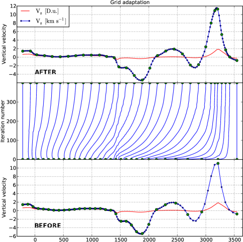
Figure 3.1: Blue lines in the bottom/top panel illustrate the vertical velocity before/after the grid points reallocation. The red lines represent the corresponding Doppler velocity ($\mathrm{\varpropto v_{z}/T^{1/2}}$), which is used to shift the nodes. We have selected $1$ grid point every $5$ (see green dots) to illustrate how they are reallocated (middle panel).

The advantages of this strategy are:

• 1) The computational implementation is easy and fast.

• 2) The procedure is flexible because $f_{k}$ can be easily redefined and adjusted with the weights $\alpha,\beta,\gamma$ .

• 3) The new grid produces a smooth variation of the physical quantities from node to node, which in general tends to diminish the corresponding numerical error gradient.

• 4) The radiative transfer equation requirements for the velocity gradients (explained in Section 4.2.3) are easily accounted for by the parameter $\beta$.

• 5) The better distribution of points allows a significant reduction of the total number of nodes without losing numerical precision in the RT solution.

The final income is that we can solve the impossible-to-converge atmosphere models in less time and with less effort.

When applied in combination with a short-characteristic method, the results given by the redistribution method depend on the spatial resolution. Taking that into account, before redistributing the grid we interpolate to a number of points that depend on the atmospheric extension in order to get a certain number of points per decade. After choosing the overall grid points, we redistribute them.

Just to put an example of the application of this method for different number of grid points, we illustrate the evolution of the Maximum Relative Change during the RT iteration in 2 different models (Fig. 3.2). Depending on the number of points per decade (p/dec), the redistribution of nodes has a better or worse effect on the convergence, in comparison with the case of no-redistribution and high resolution (red lines in Fig. 3.2). In general, $10$ p/dec seems to be insufficient for most of the expanded models, appearing a delay in convergence (blue line, upper panel, Fig. 3.2) and in many cases a lack of it. Note that these models can have shocks in higher layers, which requires more discretization points. On the contrary, in compressed atmospheres the redistribution with $10$ p/dec can give the best results (blue line, lower panel, Fig. 3.2). Redistribution with a very large number of points is inefficient in most cases (orange lines very near the red ones). It happens because redistribution plays a minor role against the decreased convergence efficiency of the DELOPAR method in very resolved grids. A trade off is represented by the green lines, corresponding to the cases with redistribution of $14$ p/dec. With this choice, we have solved the convergence problems in many highly variable models redistributing the grid points and using the less number of them possible. Tuning this procedure for any arbitrary column, we can obtain an improvement in the computational time.

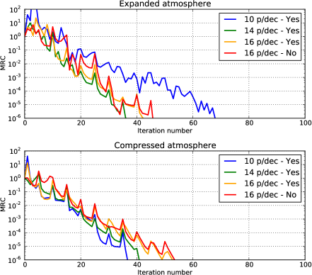
Figure 3.2: Comparison of different spatial grid interpolations for a typical expanded model (upper panel) and a typical compressed one (lower panel). The no-redistributed grid with large resolution corresponds to the red lines. The other lines are for a varying number of redistributed grid points.

3.2 Response functions in chromospheric solar models.

The response function $R^{F,X}_{\lambda}$ measures the sensitivity of a certain spectral quantity $F_{\lambda}$ to local perturbations of the physical property $X(z)$ in the model atmosphere under consideration (Landi Degl’Innocenti & Landi Degl’Innocenti, 1977; Ruiz Cobo & del Toro Iniesta, 1994) . It is defined using the following integral expression (Uitenbroek, 2006)

$$F_{\lambda}=\int^{z_{0}}_{-\infty}R^{F,X}_{\lambda}(z)X(z)dz.$$ (3.13)

$F_{\lambda}$ can be any function of the emergent Stokes parameters obtained from the model atmosphere. Equation (3.13) tell us that the response functions (RFs) behave like partial derivatives of the spectral profile ($F_{\lambda}$, or a Stokes profile in particular) with respect to a given atmospheric physical quantity at a given depth of the atmosphere. Thus, they provide a measure of the sensitivities of the observed spectral quantities to the physical magnitudes characterizing the state of the atmosphere. More precisely, they specify the heights at which a perturbation produces alterations in the spectral quantity. This is very important because, under strong non-LTE conditions (i.e., when the level populations in a transition are controlled by radiative processes or scattering), the source function at higher and less dense layers can be controlled by photons created much deeper than $\tau=1$ in the atmosphere or in hot layers well above. As the RFs account for it, they consequently provide the most reliable estimate of the heights of formation for a given model.

Due to the linearity of the integral, if the emergent $F_{\lambda}$ is recalculated after perturbing $X$ with $\Delta X$, the variation in $F_{\lambda}$ is :

$$\Delta F_{\lambda}=\int^{z_{0}}_{-\infty}R^{F,X}_{\lambda}(z)\Delta X(z)dz,$$ (3.14)

The application of a suitable perturbation allows us to calculate the response function $R$. Following Fossum & Carlsson (2005), we perturb with $\Delta X(z^{\prime})=x(z^{\prime})H(z^{\prime}-z)$, using the step function $H$, which is $0$ for $z^{\prime}>z$ and $1$ for $z^{\prime}\leq z$. Substitution of the perturbation into Equation (3.14) and subsequent differentiation yields:

$$\Delta F^{z}_{\lambda} =F^{z}_{\lambda}-F_{\lambda}=\int^{z}_{-\infty}R^{F,X}_{\lambda}(z^{\prime})x(z^{\prime})dz^{\prime},$$ (3.15a)

$$R^{F,X}_{\lambda}(z) =\frac{1}{x(z)}\frac{\mathrm{d}}{\mathrm{d}z}(\Delta F^{z}_{\lambda}).$$ (3.15b)

Following the previous equations, we have developed a program that uses Dynamic Traviata to calculate RFs of the polarization profiles in chromospheric dynamic models. The numerical evaluation of RFs can be done following these steps:

1. Synthesis of the desired spectral quantity $F_{\lambda}$ in a given unperturbed model atmosphere.

2. Considering a height $z$: perturbation of the physical quantity of interest (temperature, density, magnetic field, velocity,…) from the lowest height of the atmosphere to the height $z$ (step function) and synthesis (including calculation of the atomic density matrix) of the corresponding emergent perturbed spectrum $F^{z}_{\lambda}$.

3. Calculation of the difference $\Delta F^{z}_{\lambda}$ between both spectra.

4. Repetition of steps 2 and 3 for other height $z$, starting from the bottom upward until the last RT calculation, which is finally done perturbing all points in the atmosphere.

5. Application of Equation (3.15b).

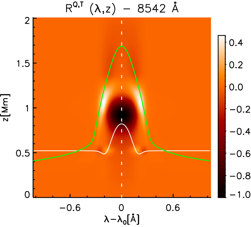
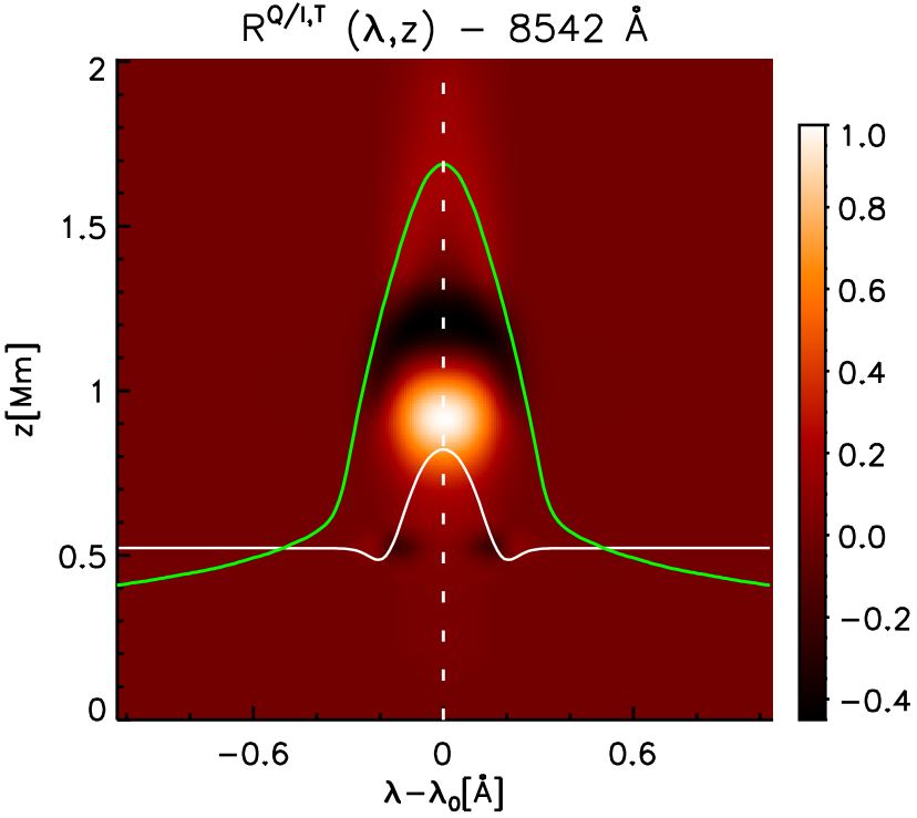
Figure 3.3: Response functions to temperature of Q (left) and Q$/$I (right) for the $8542$ Å line. The green line traces the heights of optical depth unity calculated along the line of sight ($\mu=0.1$) for each wavelength. The white line is the Q$/$I profile in arbitrary units. The RFs are normalized.

Thus, for a model atmosphere sampled at $N_{z}$ heights, the previous method complete $N_{z}+1$ full radiative transfer calculations, which can be very expensive depending on the model. An illustrative example is shown in Figure 3.3 assuming a semiempirical FAL-C model.

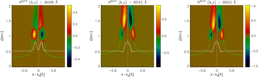
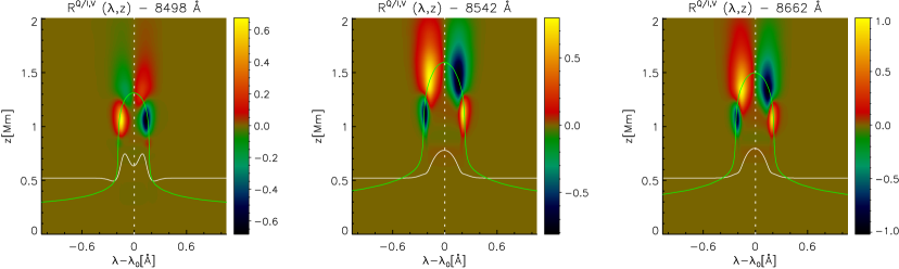
Figure 3.4: Response functions to macroscopic velocity for Q$/$I in FAL-C model with constant microturbulent velocity (upper panel) or with the original height-dependent microturbulent velocity of the model. The unperturbed macroscopic velocity is zero and the pertubation is constant and positive (hence, upward).

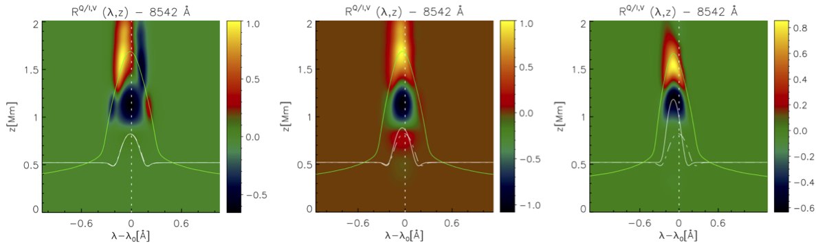
Figure 3.5: Response functions to the velocity gradient of Q$/$I using the FAL-C model with three ad-hoc velocity fields of the form $v_{z}=0.05\,v_{\rm max}\,(z[{\rm Mm}]+0.1)$ being $v_{\rm max}=1$, $10$, $30$ $\rm km\,s^{-1}$ from left to right, respectively.

It is the response function to temperature in Stokes Q (left) and in Stokes Q$/$I (right) for a same static chromospheric model. It can be seen how the line core is sensitive to perturbations in temperature at heights far below $\tau^{\rm LOS}_{\nu}=1$ (green line). For the $8542$ Å line of Caii formed in this model, the largest response takes place where the chromospheric temperature gradients increase above the minimum of temperature region. The response functions can be very useful to understand the line formation in a given model atmosphere and to characterize such a model. For instance, in Figure 3.4 we show the difference between calculations in the FAL-C model with variable (lower panels) and constant (upper panels) microturbulent velocity for the three lines of the triplet, which gives a quantitative grasp about the effect of this parameter in the radiative transfer. In this example, the response functions are computed for perturbations in bulk (macroscopic) velocity. Note that the velocity has a particularity: if we want to perturb a static model, we cannot add a perturbation being a multiplicative factor from the unperturbed model (because $v=0$). Instead, we have to consider a somehow arbitrary velocity perturbation. In our case we have simply added a constant velocity perturbation, the same for all the heights.

Although the RFs depend on the model considered, it is possible to find similarities and patterns appearing in calculations from different atmospheric models. Figure 3.5 is an example showing some common features in the RFs for three models under changes in the velocity gradient.

3.3 Tools for Principal Component Analysis.

Principal Component Analysis (PCA) is a statistical technique based on pattern recognition that is used for dimensionality reduction and signal processing. It has been applied in diverse fields of scientific research, from human face recognition (Turk & Pentland, 1991) to the classification and inversion of stellar spectra (López Ariste, 2001; Socas-Navarro, 2001). These techniques are based on the intuitive concept that a certain natural phenomena manifests itself through a corresponding finite set of basic recognizable patterns. In particular, PCA assumes that any other measurement resulting from a particular realization of that natural phenomenon can be modelled by decomposing the measurement into a linear combination of orthogonal basic patterns. Finding the most representative ones, we will be able to explain observations based on the same phenomenon and to discriminate it from the influence of other phenomena (e.g., observational noise).

Next, we explain the basic operations defining PCA applied to spectral profiles (Rees et al., 2000). We have developed a computer code that perform these operations and we have used it to analyze RT observations and theoretical results.

The application of PCA starts with the creation of an initial database of $M$ model profiles, $\phi(\lambda)$, covering in a statistical sense all possible physical states under which the measured profiles $\psi(\lambda)$ can form. Each physical state represents a model profile in the database. The model profiles can be synthetic when obtained from a physical model of the phenomenon. But they can also be obtained from a representative set of observations, so forming an observational database.

If $N$ is the number of sampling wavelengths for the model and measurement profiles, we first construct the $N\,\times\,M$ database matrix [step $1$]

$$D_{ij}=\phi_{j}(\lambda_{i})\,,\quad i=1,\ldots,N\,;\quad j=1,\ldots,M$$ (3.16)

and the associated $N\,\times\,N$ correlation matrix [step $2$],

$$\bf{C}=\bf{D}\bf{D}^{\rm T}.$$ (3.17)

Next, we have to solve the eigenvalue problem for the correlation matrix [step $3$],

$$\mathbf{C\,f}_{i}=e_{i}\mathbf{f}_{i}\,,\qquad i=1,\ldots,N$$ (3.18)

using the method of Singular Value Decomposition (SVD). The $N$-dimensional singular vectors $\mathbf{f}_{i}$ (principal components) represent a set of $N$ eigenprofiles in terms of which the profiles $\phi_{j}(\lambda)$ can be reconstructed exactly. The eigenvalues $e_{i}$ in Eq. (3.18) are ordered according to decreasing norm (hence, of decreasing significance), and they estimate the signal variance captured in the individual principal components. Usually, the first $n$ eigenprofiles, with $n\,<<\,N$, form a basis that is sufficient to reconstruct all the model profiles within the typical noise of the observations. The cumulative fractional variance explained by those few eigenvectors can be calculated with [step4]:

$$100\cdot\frac{\sum^{n}_{k=1}e_{k}}{\sum^{N}_{i=1}e_{i}}.$$ (3.19)

The basis represents the orthogonal “universal” patterns in which all profiles corresponding to the physical model adopted can be decomposed within the observational noise. These eigenprofiles are stored in the $n\,\times\,N$ matrix $\mathbf{B}$ [step $5$].

If the initial database is actually representative of the reality (either because the physical model is correct or because the observations taken to build the database are statistically well chosen), it is then unnecesary to use more than the PCA basis to approximate any other measured profile.

Thus, we can project any given measured $\psi_{j}(\lambda)$ on the basis of eigenprofiles $\mathbf{f}_{k}$, obtaining the corresponding projections $e^{j}_{k}$ with $k=1\ldots n$ [step $6$]. Such projections allow us to reconstruct the observations in the basis subspace by doing [step $7$]:

$$\bm{\psi^{\prime}}_{j}=\sum^{n}_{k=1}e^{j}_{k}\mathbf{f}_{k},$$ (3.20)

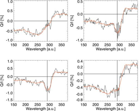
$\begin{array}[]{c}\includegraphics[width=122.85876pt]{patospca2.pdf}\\ \includegraphics[width=137.31255pt]{curvapatos.pdf}\end{array}$

Figure 3.6: Left: Examples of four PCA-reconstructed linear polarization profiles. Right upper picture: some measurements (upper row ducks) with their corresponding reconstructed images (middle row ducks) after decomposing the former set in the first five eigenvectors (lower row) of the PCA basis. Right lower picture: path followed by the projected components in the space formed by the first three eigenvectors.

where $\bm{\psi^{\prime}}_{j}\sim\bm{\psi}_{j}$, differing in an error of the order of the observational uncertainty. The finite size of the initial database implies a discrete coverage of the physical parameter space, which is the main source of numerical error in the reconstruction process.

Before performing the previous operations, our program statistically standardizes the set of model profiles to create the initial database. This is a common operation in PCA, consisting in normalizing and regularizing the mean and the statistical deviation of the profiles to be able to explain the shape of the profiles without worrying about scale factors. The program can be used to create the basis from observations of Stokes profiles or from the theoretical results of our investigation. To test it, we applied the code to spectropolarimetric observations to clean them from the noise (see figure 3.6) and we reproduced some results of Rees & Guo (2003).

3.4 The Solar Inspector

To understand the results of a radiative transfer investigation it is necessary to carry out a combined analysis of both the emergent radiative quantities (e.g., Stokes profiles) and the physical properties of the atmospheric model. In order to facilitate the analysis of the 3D models described in Chapter 6, we have developed a visual interactive application (Solar Inspector). It shows the Stokes parameters of all the considered spectral lines in combination with different maps and with the stratifications of temperature, vertical velocity and magnetic field intensity. The Stokes parameters are the result of solving the RT problem as explained in Chapter 6. In total, there are $63$ different maps. Some of them correspond to temperature, magnetic field inclination, velocity, etc. evaluated at line-center optical depth unity for every spectral line of the Ca ii IR triplet. Others are maps of Stokes profiles (or derivatives quantities) for every spectral line.

The maps correspond to the same atmospheric area and are sorted out in a specific order that allows easy and useful comparisons. The user can quickly alternate between them (see Figure 3.7) using the mouse wheel. With just a click the scroll step is modified, changing the adjacent maps to be compared. This simple strategy gives, for instance, a quick matching between features for the same map in different spectral lines or between different maps of Stokes parameters for the same spectral line. Clicking in the pixels of the maps, the corresponding atmospheric stratifications (regions A, B and C in Figure 3.7) and the emergent Stokes profiles (panels on the right in Figure 3.7) for that pixel are showed. Clicking on the different regions of the screen we can select different operations, such as overlapping Stokes profiles from different pixels to be compared or saving the actual image to a pdf file.

The program is built in Python by embedding matplotlib plots into wxPython GUIs. This allows a high-quality and versatile graphical user interface that can work interactively (without menus) using events handling. To be able to update the plots quicker while working with a large amount of data, the application have been programmed using techniques for real-time visualization.

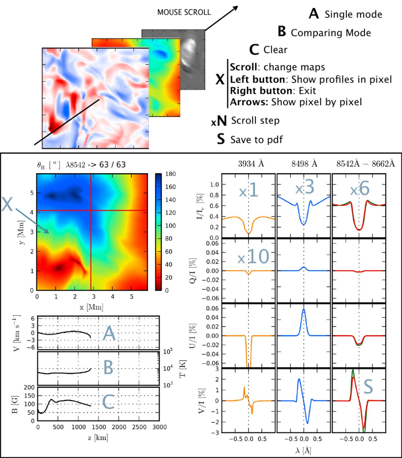
Figure 3.7: An example of a screen obtained with the Solar Inspector visualization facility. The main regions and the functionalities they offer are explained at the top of the figure.

3.5 Advanced 3D visualization with Mayavi.

Mayavi is a general-purpose scientific 3D visualization package. It uses the Visualization Toolkit (VTK), which is by far the best visualization library available (Ramachandran & Varoquaux, 2011). Unfortunately, VTK is not entirely easy to understand and many people are not interested in learning it since it has a steep learning curve. Mayavi strives to provide interfaces to VTK that make it easier to use, by applying the features of Python, a dynamical programming language, to offer simple APIs.

In short, some characteristics of Mayavi that have been relevant for the development of this thesis are:

• Rich multidimensional representation of any object and physical magnitudes able to be represented as points, lines, surfaces, volumes and fields using vectors, matrices or tensors (see examples in Figure 3.8).

• A standalone application for visualization through the so-called pipeline interface.

• Interactive 3D plots from the Python console IPython. The mlab module contained in Mayavi provides an easy way to visualize data from a script or from an interactive prompt.

• Visualization engine for embedding in user dialogs box. Mayavi allows a relatively easy interaction with other Python applications. For instance, we could use it to attach a suitable 3D visualization to the Solar Inspector application described in the previous section.

  $\begin{array}[]{cc}\framebox{\includegraphics[width=267.39877pt]{mayavi5.jpg} }&\framebox{\includegraphics[width=158.99377pt]{mayavi6.jpg} }\end{array}$

  $\begin{array}[]{cc}\framebox{\includegraphics[width=144.54pt]{mayavi3.jpg}}&\framebox{\includegraphics[width=281.85255pt]{mayavi2.jpg} }\end{array}$

  $\begin{array}[]{cc}\framebox{\includegraphics[width=216.81pt]{mayavi1.jpg} }&\framebox{\includegraphics[width=195.12877pt]{mayavi4.jpg} }\end{array}$

  Figure 3.8: Some of the visualization works done with Mayavi to analyze the 3D MHD models of Chapter 6. The model dataset has been provided by Leenaarts et al. (2009a).

When working with solar atmospheric models, importing the dataset to Mayavi is crucial but non direct. It often involves transformations and interpolations of the data to a convenient uniformly-spaced data set that is manageable by Mayavi. Distributing or creating the atmospheric models in VTK or other similar format suitable for visualization would avoid such complications. On the other hand, through third-party packages Mayavi can import IDL save files (from scipy.io.idl import readsav), which can simplify the issue.

Our experience with Mayavi indicates that it is very suitable for solar physics research. It seems to be able to create almost any data representation. In particular, we have used it to represent scalar and vector fields, surfaces, flux and field lines in a dynamic and interactive way.

To introduce the radiative information in a 3D visualization we proceed in the following way. We calculate the heights of the model where the optical depth in a certain spectral line is unity, which defines a surface in the 3D space. We plot that surface and colour it with the value of a given radiative quantity (an emergent Stokes parameter or similar). Other useful representation is to calculate the line center optical depth for a given line of sight at each point of the atmosphere and visualize it using cutting planes, isosurfaces or volumes having a variable opacity in the plot. This gives a visualization of the main formation regions for the spectral lines.

Chapter 4 Scattering Polarization with Velocity Gradients.

In this chapter, we present the effects that gradients in the macroscopic vertical velocity field have on the non-magnetic scattering polarization signals, establishing the basis for other cases. We show that the solar plasma velocity gradients have a significant effect on the linear polarization produced by scattering in chromospheric spectral lines. In particular, we calculate the impact of velocity gradients on the anisotropy of the radiation field and on the ensuing fractional alignment of the Ca ii levels, and how they can lead to an enhancement of the zero-field linear polarization signals. This theoretical investigation remarks the importance of knowing the dynamical state of the solar atmosphere in order to correctly interpret spectropolarimetric measurements, which is important, among other things, for establishing a suitable zero field reference case to infer magnetic fields via the Hanle effect.

4.1 Introduction

Over the last few years it has become increasingly clear that the determination of the magnetic field in the “quiet” solar chromosphere requires measuring and interpreting the linear polarization profiles produced by scattering in strong spectral lines, such as H_α and the 8542 Å line of the infrared triplet of Ca ii (e.g., see Trujillo Bueno, 2010; Uitenbroek, 2011). In these chromospheric lines, the maximum fractional linear polarization signal occurs at the center of the spectral line under consideration, where the Hanle effect (i.e., the magnetic-field-induced modification of the scattering line polarization) operates (Stenflo et al., 1998). Since the opacity at the center of such chromospheric lines is very significant, it is natural to find that the response function of the emergent scattering polarization to magnetic field perturbations peaks in the upper chromosphere (Ŝtêpán & Trujillo Bueno, 2010). This contrasts with the circular polarization signal caused by the Zeeman effect whose response function peaks at significantly lower atmospheric heights (Socas-Navarro & Uitenbroek, 2004). Of particular importance for developing the Hanle effect as a diagnostic tool of chromospheric magnetism is to understand and calculate reliably the linear polarization profiles corresponding to the zero-field reference case.

The physical origin of the scattering line polarization is atomic level polarization (that is, population imbalances and/or coherence between the magnetic sublevels of a degenerate level with total angular momentum $J$). Atomic polarization, in turn, is induced by anisotropic radiation pumping, which can be particularly efficient in the low-density regions of stellar atmospheres where the depolarizing role of elastic collisions tends to be negligible. The larger the anisotropy of the incident field, the larger the induced atomic level polarization, and the larger the amplitude of the emergent linear polarization.

The degree of anisotropy of the spectral line radiation within the solar atmosphere depends on the center-to-limb variation (CLV) of the incident intensity. In a static model atmosphere the CLV of the incident intensity is established by the gradient of the source function of the spectral line under consideration (Trujillo Bueno, 2001; Landi Degl’Innocenti & Landolfi, 2004). However, stellar chromospheres are highly dynamic systems, with shocks and wave motions (e.g., Carlsson & Stein, 1997). The ensuing macroscopic velocity gradients and Doppler shifts might have a significant impact on the radiation field anisotropy and, consequently, on the emergent polarization profiles. Therefore, it is important to investigate the extent to which macroscopic velocity gradients may modify the amplitude and shape of the emergent linear polarization profiles produced by optically pumped atoms in the solar atmosphere. The main aim of this chapter is to explain why atmospheric velocity gradients may modify the anisotropy of the spectral line radiation and, therefore, the emergent scattering line polarization. We also aim at evaluating, with the help of ad-hoc velocity fields introduced in a semi-empirical solar model atmosphere, their possible impact on the scattering polarization of the IR triplet of Ca ii. A recent investigation by Manso Sainz & Trujillo Bueno (2010), based on radiative transfer calculations in static model atmospheres, shows why the differential Hanle effect in these lines is of great potential interest for the exploration of chromospheric magnetism.

4.2 Formulation of the problem and relevant equations

4.2.1 The atomic model and the statistical equilibrium equations (SEE)

We assume an atomic model consisting of the five lowest energetic, fine structure levels of Ca ii (see Figure 1). The excitation state of the atomic system is given by the populations of its 18 magnetic sublevels and the coherences among them. We neglect coherences between different energy levels of the same term (multilevel approximation). Moreover, since the problem we consider here (plane-parallel, non-magnetic atmosphere with vertical velocity fields) is axially symmetric around the vertical direction, no coherences between different magnetic sublevels exist when the symmetry axis is taken for quantizing the angular momentum. We use the multipolar components of each $J$-level,

$$\rho^{K}_{0}=\sum_{M=-J}^{+J}(-1)^{J-M}\sqrt{2K+1}\left(\begin{array}[]{ccc}J&J&K\\ M&-M&0\end{array}\right)N_{M},$$ (4.1)

where $K=0,...,2J$, $N_{M}$ is the population of the sublevel with magnetic quantum number $M$, and the symbol between brackets is the Wigner $3j$-symbol (e.g., Brink & Satchler 1968). Due to the symmetry of the scattering process (no magnetic field, no polarized incident radiation in the atmosphere’s boundaries), in a given level $N_{+M}=N_{-M}$, and the excitation state of the system is described by just 9 independent sublevel populations. Consequently, odd-$K$ elements (orientation components) in Eq. (4.1) vanish for all five levels, and the only independent variables of the problem in the spherical components formalism are the total populations of the five levels ($\sqrt{2J+1}\rho^{0}_{0}$); the alignment components ($\rho^{2}_{0}$) of levels 2, 3, and 5; and $\rho^{4}_{0}$ of level 3, whose role is negligible for our problem.

The statistical equilibrium equations accounting for the radiative and collisional excitations and deexcitations in the 5-level system of Fig. 4.1 are given explicitly in Manso Sainz & Trujillo Bueno (2010). We have particularized them to the no-coherence case (only $\rho^{K}_{0}$ elements) in Appendix A.2. The statistical equilibrium equations for the $\rho^{0}_{0}$ components contain terms that are equal to those appearing in the statistical equilibrium equations for the populations in a standard (no polarization) NLTE problem (e.g., Mihalas 1978), plus higher order terms $\sim J^{2}_{0}\rho^{2}_{0}$ (see Eqs. A.9-A.13). The statistical equilibrium equations for the alignment ($\rho^{2}_{0}$ components) are formally similar to the ones for the populations with additional terms $\sim J^{2}_{0}\rho^{0}_{0}$ accounting for the generation of alignment from the anisotropy of the radiation field, and (negligible) higher order terms $\sim J^{2}_{0}\rho^{2}_{0}$ and $J^{2}_{0}\rho^{4}_{0}$ (see Equations (A.14), (A.15) and (A.16)). These equations are expressed in the atom reference frame (comoving system).

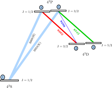
Figure 4.1: Atomic model with energy levels for Caii. The labels indicate the spectroscopic terms. Numbers inside blue filled circles identificate each level. Solid lines connecting levels show the allowed radiative transitions and the numbers at the middle of each segment are their wavelength in Å. The wider the width of each connecting line the larger the spontaneous emission rate $A_{ul}$ of the transition. Atomic data for each spectral line are shown in Table 4.1.

$\lambda$ (Å )	$u$	${\ell}$	$A_{u{\ell}}$ (s-1)	$w_{J_{\ell}J_{u}}^{(2)}$	$w_{J_{u}J_{\ell}}^{(2)}$
Allowed transitions
3934 (K)	5	1	$1.4\times 10^{8}$	$0$	$\sqrt{2}/2$
3969 (H)	4	1	$1.4\times 10^{8}$	$0$	$0$
8498	5	2	$1.11\times 10^{6}$	$-2\sqrt{2}/5$	$-2\sqrt{2}/5$
8542	5	3	$9.6\times 10^{6}$	$\sqrt{7}/5$	$\sqrt{2}/10$
8662	4	2	$1.06\times 10^{7}$	$\sqrt{2}/2$	$0$

Table 4.1: Short list of Ca ii atomic data parameters. From left to right: the central wavelength, the upper and the lower level of each transition, the radiative rates from NIST atomic spectra database (http://www.nist.gov/physlab/data/asd.cfm) and the atomic polarizability coefficients introduced by Landi Degl’Innocenti (1984).

Since the radiation field is axially symmetric, just two radiation field tensor elements ($J^{0}_{0}$ and $J^{2}_{0}$) are necessary to describe the symmetry properties of the spectral line radiation.

Let $I(\nu,\mu)$ and $Q(\nu,\mu)$ be the Stokes parameters expressed in the observer’s frame at a given height $z$, where $\nu$ is the frequency, $\mu=\cos\theta$ and $\theta$ is the angle that the ray forms with the vertical direction. Then, the corresponding values seen by a comoving frame with vertical velocity $v_{z}$ with respect to the observer’s frame are $I^{\prime}(\nu^{\prime},\mu)=I(\nu,\mu)$ and $Q^{\prime}(\nu^{\prime},\mu)=Q(\nu,\mu)$, where $\nu^{\prime}=\nu(1-v_{z}\mu/c)$ and $\nu=\nu^{\prime}(1+v_{z}\mu/c)$ (to first order in $v_{z}/c$). Therefore, the mean intensity at the considered height, can be expressed from one or another reference frame as:

$$\bar{J}^{0}_{0} =\frac{1}{2}\int d\nu\int_{-1}^{1}d\mu\phi^{\prime}_{\ell u}(\nu,\mu)I(\nu,\mu)$$

$$=\frac{1}{2}\int d\nu^{\prime}\int_{-1}^{1}d\mu\phi_{\ell u}(\nu^{\prime})I(\nu^{\prime}(1+v_{z}\mu/c),\mu),$$ (4.2)

where $\phi_{\ell u}(\nu)$ is the absorption profile (e.g., for a Gaussian profile, we would have $\phi_{\ell u}(\nu)=\pi^{-1/2}{\Delta\nu_{D}}^{-1}\exp(-(\nu-\nu_{0})^{2}/{\Delta\nu_{D}}^{2})$, with $\nu_{0}$ the central line frequency and $\Delta\nu_{D}$ the Doppler width) and $\phi^{\prime}_{\ell u}(\nu,\mu)=\phi_{\ell u}(\nu(1-v_{z}\mu/c))$, with $v_{z}>0$ for upflowing material. Analogously, the anisotropy in the observer’s frame:

$$\bar{J}^{2}_{0} = \frac{1}{4\sqrt{2}}\int d\nu\int_{-1}^{1}d\mu\phi_{\ell u}^{\prime}(\mu,\nu)$$ (4.3)

$$\times [(3\mu^{2}-1)I(\nu,\mu)+3(1-\mu^{2})Q(\nu,\mu)],$$

The important quantity that controls the ability of an anisotropic radiation field to generate atomic polarization is the line anisotropy factor for each transition, which can be calculated as:

$$w_{\mathrm{line}}={\sqrt{2}}\frac{\bar{J}^{2}_{0}}{\bar{J}^{0}_{0}}.$$ (4.4)

Its range goes from $w_{\mathrm{line}}=-0.5$ (for an azimuthally independent radiation field coming entirely from the horizontal plane) to $\sc w_{\mathrm{line}}=1$ (for a collimated vertical beam).

4.2.2 The radiative transfer equations (RTE)

Due to symmetry, in a non-magnetized plane-parallel medium with a vertical velocity field, light can only be linearly polarized parallel or perpendicularly to the stellar limb. Therefore, chosing the reference direction for positive $Q$ parallel to the limb, the only non-vanishing Stokes parameters are $I$ and $Q$, and they satisfy the following radiative transfer equations:

$$\frac{\rm d}{{\rm d}s}I =\epsilon_{I}-\eta_{I}I-\eta_{Q}Q,$$ (4.5a)

$$\frac{\rm d}{{\rm d}s}Q =\epsilon_{Q}-\eta_{Q}I-\eta_{I}Q,$$ (4.5b)

where $s$ is the distance along the ray. The absorption and emission coefficients are (Manso Sainz & Trujillo Bueno, 2010):

$$\epsilon_{I} =\,\epsilon_{I}^{\rm cont}+\epsilon_{I}^{\rm line}$$

$$=\,{\eta_{I}}^{\rm cont}B_{\nu}+\epsilon_{0}\left[\rho^{0}_{0}(u)+w_{J_{u}J_{\ell}}^{(2)}\frac{1}{2\sqrt{2}}(3\mu^{2}-1)\rho^{2}_{0}(u)\right],$$ (4.6a)

$$\eta_{I} =\,\eta_{I}^{\rm cont}+\eta_{I}^{\rm line}$$

$$=\,{\eta_{I}}^{\rm cont}+\eta_{0}\left[\rho^{0}_{0}(\ell)+w_{J_{\ell}J_{u}}^{(2)}\frac{1}{2\sqrt{2}}(3\mu^{2}-1)\rho^{2}_{0}(\ell)\right],$$ (4.6b)

$$\epsilon_{Q}\,=\,\epsilon^{\rm line}_{Q}\,=\,\epsilon_{0}w_{J_{u}J_{\ell}}^{(2)}\frac{3}{2\sqrt{2}}(1-\mu^{2})\rho^{2}_{0}(u),$$ (4.7a)

$$\eta_{Q}\,=\,\eta^{\rm line}_{Q}\,=\,\eta_{0}w_{J_{\ell}J_{u}}^{(2)}\frac{3}{2\sqrt{2}}(1-\mu^{2})\rho^{2}_{0}(\ell),$$ (4.7b)

where ${\eta_{I}}^{\rm cont}$ and ${\epsilon_{I}}^{\rm cont}$ are the continuum absorption and emission coefficients for intensity, respectively. Likewise, $\eta_{I}^{\mathrm{line}}$ and $\eta_{Q}^{\mathrm{line}}$ are the line absorption coefficients for Stokes $I$ and $Q$, respectively, while $\epsilon_{I}^{\mathrm{line}}$ and $\epsilon_{Q}^{\mathrm{line}}$ are the line emission coefficients for Stokes $I$ and $Q$, respectively. The coefficients $w_{J_{\ell}J_{u}}^{(2)}$ and $w_{J_{u}J_{\ell}}^{(2)}$ depend only on the transition and are detailed in Table (4.1).The subscripts $u$ and $\ell$ refer to the upper and lower level of the transition considered, respectively, and $B_{\nu}$ is the Planck function at the central frequency $\nu_{0}$ of the transition. Note also that:

$$\epsilon_{0}=\frac{h\nu}{4\pi}A_{u{\ell}}{\phi^{\prime}_{\ell u}(\mu,\nu)}{\cal N}\sqrt{2J_{u}+1},$$ (4.8a)

$$\eta_{0}=\frac{h\nu}{4\pi}B_{{\ell}u}{\phi^{\prime}_{\ell u}(\mu,\nu)}{\cal N}\sqrt{2J_{\ell}+1},$$ (4.8b)

where $\cal N$ is the total number of atoms per unit volume.

With the total absorption coefficient for the intensity, the line of sight (los) optical depth for each frequency is calculated by the following integral along the ray:

$$\tau^{\rm los}_{\nu}=-\int\eta_{I}(\mu^{\rm los},\nu)\frac{dz}{\mu^{\rm los}}$$ (4.9)

4.2.3 Numerical method

The solution to the non-LTE problem of the second kind considered here (the self-consistent solution of the statistical equilibrium equations for the density matrix elements together with the radiative transfer equations for the Stokes parameters) is carried out by generalizing the computer program developed by Manso Sainz & Trujillo Bueno (2003a), to allow for radial macroscopic velocity fields (see Sec. 3.1.2). For integrating the RTE, a parabolic short-characteristics scheme (Kunasz & Auer, 1988) is used. At each iterative step, the radiative transfer equation is solved, and $\bar{J}^{0}_{0}$ and $\bar{J}^{2}_{0}$ are computed and used to solve the SEE following the accelerated Lambda iteration method outlined in Sec. 3.1.1. Once the solution for the multipolar components of the density matrix is consistently reached, the emergent Stokes parameters are calculated for the desired line of sight, which in all the figures of this chapter is $\mu=0.1$. This final step is done increasing the frequency grid resolution to a large value in order to correctly sample the small features and peaks of the emergent profiles.

Some technical considerations have to be kept in mind for the treatment of velocity fields (see Sec. 3.1.2). Due to the presence of Doppler shifts, the wavelength axis used to compute $\bar{J}^{0}_{0}$ and $\bar{J}^{2}_{0}$ must include the required extension and resolution, because the spectral line radiation may be now shifted and asymmetric. In our strategy for the wavelength grid, the resolution is larger in the core than in the wings, keeping the same wavelength grid for all heights.

The cutoff wavelength for the core (where resolution is appreciably higher) is dictated by the maximum expected Doppler shift. Thus, the core bandwidth is estimated allowing for a range of $2V_{\rm{max}}$ around the zero velocity central wavelength of the lines, with $V_{\rm{max}}$ the maximum velocity found in the atmosphere (in Doppler units). Apart from that, a minimum typical resolution for the core is set to 2 points per Doppler width ($\Delta\nu_{D}$). Then, the height with the smallest Doppler width determines the core resolution, and the height with the maximum macro-velocity states its bandwidth.

Furthermore, as frequencies and angles are inextricably entangled (through terms $\nu-v_{z}\mu\nu/c$ appearing in the absorption/emission profiles due to the Doppler effect, like in Eq. (4.2.1)), the maximum angular increment ($\Delta\mu_{\rm{max}}$) is restricted by the maximum frequency increment ($\Delta x_{\rm{max}}\thickapprox 1/2$, in Doppler units). Thus, it must occur that $\Delta\mu_{\rm{max}}\cdot V_{\rm{max}}\leq 1/2$. In the worst case, the maximum allowed angular increment will be smaller (more angular resolution needed) when the maximum vertical velocity increases. Besides this consideration, the maximum angular increment could be even more demanding because of the high sensitivity of the polarization profiles to the angular discretization.

Finally, the depth grid must be fine enough, in such a way that the maximum difference in velocity between consecutive points is not too large, the typical difference being equal to half the Doppler width ($|V(z_{i})-V(z_{i-1})|\leq 1/2$). If the difference is larger, the absorption/emission profiles would change abruptly with height, producing imprecisions in the optical depth increments (Mihalas, 1978).

4.3 Effect of a velocity gradient on the radiation field.

As we shall see, the presence of a vertical velocity gradient in an atmosphere enhances the anisotropy of the radiation field and, hence, of the scattering line polarization patterns. The fundamental process underlying this mechanism can be simply understood with the following basic examples.

4.3.1 Anisotropy seen by a moving scatterer.

Consider an absorption spectral line with a Gaussian profile emerging from a static atmosphere with a linear limb darkening law,

$$I(\nu,\mu)=I^{(0)}(1-u+u\mu)[1-a\exp(-(\frac{\nu-\nu_{0}}{w})^{2})],$$ (4.10)

where $I^{(0)}$ is the continuum intensity at disk center, $u$ is the limb darkening coefficient, $a<1$ measures the intensity depression of the line, and $w$ its width. In this approximation we assume that all the parameters are constant. Now imagine that, at the top of the atmosphere, there is a thin cloud scattering the incident light given by Eq. (4.10) and moving radially at velocity $v_{z}$ with respect to the bottom layers of the atmosphere, supposed static. We will assume that the absorption profile is Gaussian (dominated by Doppler broadening), with width $\Delta\nu_{D}$. When $\Delta\nu_{D}\ll w$, the incident spectral line radiation is much broader than the absorption profile (in fact, for $\alpha=\Delta\nu_{D}/w=0$ the absorption profile is formally a Dirac-$\delta$ function). Then, from Equations (4.2.1)-(4.3) we can derive explicit expressions for the mean intensity and anisotropy of the radiation field as a function of the scatterer velocity (see Appendix A.1): $\bar{J}^{0}_{0}={\cal I}_{0}(\alpha;\xi)/2$, $\bar{J}^{2}_{0}={\cal I}_{2}(\alpha;\xi)/4\sqrt{2}$, where the ${\cal I}_{0,2}$ functions are defined by Equations (A.1)-(A.1). The behavior of $\bar{J}^{0}_{0}$ and $\bar{J}^{2}_{0}$ with the adimensional velocity $\xi=v_{z}\nu_{0}/(cw)$ (Figure 4.2), is most clearly illustrated in their asymptotic limits at low velocities:

$$\bar{J}^{0}_{0} =\frac{1}{4}(1-\frac{a}{\sqrt{1+\alpha^{2}}})(2-u)$$

$$+ \frac{a(4-u)}{12(1+\alpha^{2})^{3/2}}\xi^{2}+{\rm O}(\xi^{3}),$$ (4.11)

$$\sqrt{2}\frac{\bar{J}^{2}_{0}}{\bar{J}^{0}_{0}} =\frac{u}{4(2-u)}$$

$$+ \frac{a(64-56u+7u^{2})}{120(2-u)^{2}(1+\alpha^{2})(\sqrt{1+\alpha^{2}}-a)}\xi^{2}+{\rm O}(\xi^{3}).$$ (4.12)

Equation (4.11) shows that, for an absorption line ($a>0$), $\bar{J}^{0}_{0}$ is always increasing with the velocity since the coefficient of $\xi^{2}$ is positive, regardless of the sign of $v_{z}$ (i.e., regardless of whether the scatterers move upwards or downwards); if the line is in emission ($a<0$), $\bar{J}^{0}_{0}$ monotonically decreases. These are the Doppler brightening and Doppler dimming effects (e.g., Landi Degl’Innocenti & Landolfi, 2004). An analogous analysis applies to $\bar{J}^{2}_{0}$ (Eq. 4.12). Note that, in the absence of limb darkening ($u=0$), the anisotropy vanishes in a static atmosphere, while the mere presence of a relative velocity between the scatterers and the underlying static atmosphere induces anisotropy in the radiation field —hence, a polarization signal. A real atmosphere could then be understood as a superposition of scatterers that modify the anisotropy depending on the local velocity gradient and the illumination received from lower shells. An interesting discussion on the effect of velocities with directions other than radial can be found in Section 12.4 of Landi Degl’Innocenti & Landolfi (2004) .

Figure 4.2: $\bar{J}^{0}_{0}/I^{(0)}$ (left panel) and $\sqrt{2}\bar{J}^{2}_{0}/\bar{J}^{0}_{0}$ (right panel) as a function of the adimensional velocity $\xi$ calculated using an incident line profile as in Eq. (4.10) with $u=0.3$ and $a=0.4$ or 0.8 (see labels). Dotted lines have been computed for the case of an infinitely sharp absorption profile ($\alpha=0$). Solid lines refer to the case $\alpha=0.9$ (non saturated line). The case with no limb darkening ($u=0$) and $a=0.4$ has been plotted for comparison (dashed lines).

Figure 4.3: Adimensional velocity fields considered in this section. They are parameterized by the limiting value at small optical depths (labels) and by the location in optical depth of the largest velocity gradient region (vertical lines marking $\tau_{0}$). Solid lines: $\tau_{0}=1$. Dotted lines: $\tau_{0}=100$.

Figure 4.4: $\bar{J}^{0}_{0}$ (left panel) and $\sqrt{2}\bar{J}^{2}_{0}/\bar{J}^{0}_{0}$ (right panel) as a function of the integrated static line opacity ($\tau_{l}$) in an expanding atmosphere with $S=S^{(0)}(1+\beta\tau_{l})$ and different velocity stratifications $\xi=\xi_{0}/(1+\tau_{l}/\tau_{0})$ (see Fig. 4.3). The parameters used in this plot are $\beta=3/2$ and $\kappa_{c}/\kappa_{l}=10^{-4}$. The labels indicate the value of $\xi_{0}$. Solid lines correspond to $\tau_{0}=1$ while dotted lines refer to $\tau_{0}=100$.

Clearly, all the above discussion depends on the Doppler shift induced by the velocity $v_{z}$ normalized to the width of the spectral line, i.e., on $\xi$. A large velocity gradient on a broad line can have the same effect as that of a smaller velocity gradient on a narrow line. This is important to be kept in mind since the response of different spectral lines to the same velocity gradient will be different, what can help us to decipher the velocity stratification. Even different spectral lines belonging to the same atomic species may have very different widths, as for example, the Ca ii IR triplet and the UV doublet studied in the next section.

4.3.2 Calculations in a Milne-Eddington model.

The discussion above explains the basic mechanism by means of which a velocity gradient enhances the anisotropy of the radiation field. Now we can get further insight on the structure of the radiation field within an atmosphere with velocity gradients from just the formal solution of the RT equation for the intensity (e.g., Mihalas, 1978). As before, we neglect effects due to polarization and $J^{0}_{0}$ and $J^{2}_{0}$ are calculated from Stokes $I$ alone. We consider a semi-infinite, plane-parallel atmosphere with a source function $S=S_{0}(1+\beta\tau_{l})$, where $\tau_{l}$ is the integrated line optical depth in the static limit (hence, the element of optical depth $d\tau_{\nu}=(r+\phi[\nu(1-v_{z}(\tau_{l})\mu/c)])d\tau_{l}$, where $r=\kappa_{c}/\kappa_{l}$ is the ratio of continuum to line opacity). We begin by considering a vertical velocity field $v_{z}(\tau_{l})=v_{0}/[1+(\tau_{l}/\tau_{0})]$ (positive away from the star), shown in Fig. 4.3. Equivalently, we may express the velocity in adimensional terms by using $\xi=(\nu_{0}/c)v_{z}/\Delta\nu_{D}$ (the width $\Delta\nu_{D}$ of the Gaussian absorption profile is assumed to be constant with depth). The parameter $\tau_{0}$ fixes the position of the maximum velocity gradient. Note that the wavelength dependence of the Doppler effect ($\Delta\lambda_{z}=\lambda_{0}v_{z}/c$) is cancelled in the adimensional problem, where velocities are measured in Doppler units. It is easy to calculate numerically $I_{z}(\nu,\mu)$ at every point in the atmosphere and thus, the mean intensity and anisotropy of the radiation field (Figure 4.4).

The rise in $\bar{J}^{0}_{0}$ in higher layers with respect to the static case corresponds to the Doppler brightening discussed above. Thanks to the Doppler shifts, the atoms see more and more of the brighter continuum below, which enhances $\bar{J}^{0}_{0}$. When the maximum velocity gradient takes place at optically thick enough layers ($\tau_{0}\gtrsim 1$), $\bar{J^{0}_{0}}$ is also larger than for the static case, but it decreases monotonically with height in the atmosphere ($\tau_{0}=10^{2}$, dotted lines in left panel of Fig. 4.4). Note that the important quantity that modulates the increase in $\bar{J^{0}_{0}}$ is not the maximum velocity but the velocity gradient (difference in velocity between optically thick and optically thin parts of the atmosphere). The larger the gradient, the more pronounced the radiative decoupling is between different heights. An extreme example of such radiative decoupling could be found in supernovae explosions, where the vertical velocity gradients are huge.

In our case (vertical motions), the Doppler brightening implies an enhancement of the contribution of vertical radiation to Eq. (4.3) with respect to the horizontal radiation, with the latter remaining almost equal to the static case (no horizontal motions, no horizontal Doppler brightening). This velocity-induced limb darkening is the origin of the anisotropy enhancement.

However, note that the maximum anisotropy does not rise indefinitely when increasing the maximum velocity. If the velocity gradient in units of the Doppler width is larger than $\sim 3$ (see curves for $\xi_{\rm{max}}=5$ in Fig. 4.4), the anisotropy at the surface saturates and decreases (even below the curves corresponding to shorter velocity gradients). It forms a bump around $\tau_{l}=1$ when the maximum velocity gradient is taking place at low density layers ($\tau_{0}\lesssim 1$). This behavior can be understood using Eq. (4.3). When $\xi_{\rm{max}}\lesssim 3$, an increment in $\xi_{\rm{max}}$ entails a rise in $\bar{J}^{0}_{0}$, $\bar{J}^{2}_{0}$ and $\bar{J}^{2}_{0}/\bar{J}^{0}_{0}$ ($w_{\rm{line}}$) in the upper atmosphere, what means that the velocity gradients enhance the imbalance between vertical and horizontal radiation. However, if $\xi_{\rm{max}}$ is above that threshold, $\bar{J}^{0}_{0}$ and $\bar{J}^{2}_{0}$ rise, but the ratio $\bar{J}^{2}_{0}/\bar{J}^{0}_{0}$ saturates and diminishes. The reason is that a large velocity gradient makes the absorption profiles associated with almost horizontal outgoing rays ($0<\mu<1/\sqrt{3}$) to be so much shifted that they also capture the background continuum radiation. Their contributions are negative to the angular integral of $\bar{J}^{2}_{0}$ but positive for $\bar{J}^{0}_{0}$.

Separating the contributions of rays with angles in the range $1/\sqrt{3}<|\mu|<1$ (that we refer to with the label $+$) and angles in the range $0<|\mu|<1/\sqrt{3}$ (that we refer to with the label $-$), the line anisotropy can be written as $w_{\rm{line}}=w^{+}_{\rm{line}}+w^{-}_{\rm{line}}=\bar{J}^{2+}_{0}/\bar{J}^{0}_{0}-|\bar{J}^{2-}_{0}|/\bar{J}^{0}_{0}$. Here, $\bar{J}^{0}_{0}$ and $\bar{J}^{2+}_{0}$ grow always with $\xi_{\rm{max}}$, but $|\bar{J}^{2-}_{0}|$ only grows appreciably when $\xi_{\rm{max}}\gtrsim 3$. Therefore, although $w_{\rm{line}}$ increases for all velocity gradients, its enhancement is smaller for large velocity gradients than for smaller ones. This effect occurs as well when motions take place deeper ($\tau_{0}\gtrsim 1$) but it is less important and the anisotropy bump and saturation are reduced.

For the considered velocity fields (with a negligible gradient in the upper atmosphere), $\bar{J}^{0}_{0}$ and $\bar{J}^{2}_{0}$ reach an asymptotic value in optically thin regions. It does not occur if the velocity gradient is not zero at those layers. In any case, the presence of a large anisotropy in optically thin regions barely affects the emergent linear polarization profiles.

4.3.3 Two-level model atom in dynamic atmospheres.

Before going to a more realistic case, a final illustrative example is considered. In this case, we assume the same parameterization of the velocities than in the previous example, but now we solve the complete iterative RT problem with a two-level atom model and a specific temperature stratification. Consequently, the source function and the anisotropy are consistently obtained in a moving atmosphere. The intensity source function is $S_{I}=r_{\nu\mu}S^{\rm{line}}_{I}+(1-r_{\nu\mu})B$ (e.g., Rybicki & Hummer, 1991), with $r_{\nu\mu}=\phi^{\prime}_{\ell u}(\nu,\mu)/(r_{c}+\phi^{\prime}_{\ell u}(\nu,\mu))$ and the expression for the line source function remains formally equal to that of the static case, being $S^{\rm{line}}_{I}=(1-\epsilon)\bar{J}^{0}_{0}+\epsilon B$, where $B$ is the imposed Planck function, $\epsilon$ is the inelastic collisional parameter and $\bar{J}^{0}_{0}$ is calculated with Eq. (4.2.1).

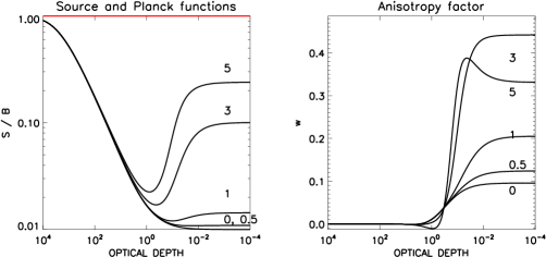
Figure 4.5: Same as Fig. 4.4 for an isothermal moving atmosphere with a two-level atom model using the velocity fields of Fig. 4.3. We assume a very strong line ($r_{c}=0$) and $\epsilon=10^{-4}$. Left panel: the Doppler brightening effect increases the surface source function value. In a two-level model atom in a static atmosphere (label 0) this value follows the well known expression $S(0)=\sqrt{\epsilon}B$. The vertical axis is in units of the Planck function. Right panel: we show the amplification of the radiation field anisotropy when the velocity gradient increases. The curve labeled with “5” shows the saturation of the anisotropy and the bump produced by the strong velocity gradient taking place in optically thin regions.

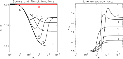
Figure 4.6: Calculations in isothermal two-level atom moving atmospheres with $\xi_{max}=5$ . We assume a very strong line ($r_{c}=0$) and $\epsilon=10^{-4}$. The highest velocity gradient occur at $\tau_{l}=\tau_{0}=100,10,1,0.1,0.01$ for a, b, c, d and e, respectively. The case f corresponds to the solution in a static atmosphere. The vertical dotted line marks the position of $\tau_{l}=0.1$.

The qualitative behavior explained in the previous subsection is maintained in these two-level atom calculations. For small $\epsilon$ values (large NLTE effects), the source function $S_{I}\thickapprox\bar{J}^{0}_{0}$ shows Doppler brightening effects and its surface value depends on the maximum velocity gradient and on the maximum background continuum set by the photospheric conditions (upper panel in Fig. 4.5). The anisotropy rises proportionally to the velocity gradient until a saturation occurs (lower panel in Fig. 4.5). A similar behavior is found when the maximum velocity gradient occurs higher in the atmosphere (see Fig. 4.6).

In a static atmosphere, the radiation field anisotropy is dominated by the presence of gradients in the intensity source function (Trujillo Bueno et al., 2001; Landi Degl’Innocenti & Landolfi, 2004), which can be modified via the Planck function (equivalently, the temperature). In the dynamical case that we are dealing with, the slope of the source function is also modified due to the existence of velocity gradients thanks to the frequency-decoupling caused by relative motions between absorption profiles (Doppler brightening). In general, both mechanisms act together (velocity-induced and temperature-induced modification of the source function gradient) and the ensuing anisotropy and the emergent linear polarization profiles are modified accordingly.

It is important to note that the adimensional velocity $\xi$ depends both on the velocity and also on the line Doppler width because $\xi(\tau)=\delta\nu/\Delta\nu_{D}=v_{z}/\sqrt{2k_{B}T/m}$, with $k_{B}$ the Boltzmann constant, $T$ the temperature and $m$ the mass of the atom. In the photosphere, where velocities are much lower than in the chomosphere, $\xi$ is expected to be negligible. In the chromosphere, plasma motions are important and the temperature is still comparable to that of the photosphere, inducing $\xi$ to be controlled by the velocity field. However, for layers in the transition region and above, the high temperatures reduce the value of $\xi$. In any case, at these heights, the density is so low that, although $\xi$ (and consequently the anisotropy) could have a highly variable behavior, the emergent polarization profiles of chromospheric lines will not be sensitive to them.

4.4 Results for the Ca ii IR Triplet

Now, we study the effect of the velocity field on a multilevel atomic system in a semiempirical atmospheric model, within the framework described in Sec. 4.2. We consider the formation of the scattering polarization pattern of the Ca ii infrared triplet in the FAL-C model of Fontenla et al. (1993) in the presence of vertical velocity fields ($\vec{v}=v_{z}(z)\vec{k}$, with $\vec{k}$ the unit vector along the vertical pointing upwards). We will assume a constant microturbulent velocity field of 3.5 km s^-1, which is a representative value for the region of formation that gives a correct broadening of the triplet profiles.

4.4.1 Behavior of the anisotropy in the Ca ii IR triplet

For simplicity, we set linear velocity fields (constant velocity gradient along z) between $z=-100$ and 2150  km (see Fig. 4.7). Consequently, the adimensional velocity field $\xi_{z}$ has a non-monotonic behavior due to its dependence on the temperature (upper right panel in Fig. 4.7). In the chromosphere, where the Ca ii triplet lines form, $\xi_{z}$ is dominated by the macroscopic motions. Here, the velocity gradients produce variations in the anisotropy of the triplet lines that agree with the behavior outlined in the previous sections. Namely, an amplification and a subsequent saturation of the anisotropy factor due to the significant velocity gradient at those heights (see the lower panels and middle right panel in Fig. 4.7). Above the chromosphere, on the contrary, the temperature dominates ($\xi_{z}$ stabilizes and diminishes) and the anisotropy slightly decreases with height. If the (adimensional) velocity gradient is negligible where the line forms (around $\tau^{\mathrm{los}}_{\nu_{0}}\thicksim 1$), the anisotropy remains unaffected. Otherwise, if a spectral line forms at very hot layers, where the absorption profiles are wider and their sensitivity to the velocity gradients is lower, the Doppler brightening will not be so efficient amplifying the anisotropy. This is the case of the anisotropy of the Ca ii K line (middle left panel in Fig. 4.7). Compare how the slope of $\xi_{z}$ is smaller where the Ca ii K line forms (black line on Fig. 4.7) than where the triplet lines do. Consequently, the enhancement of the line anisotropy through the presence of velocity gradients in this line is reduced.

All our calculations demonstrate that the anisotropy in the Ca ii IR triplet can be amplified through chromospheric vertical velocity gradients. This results suggest that the same occurs with the ensuing linear polarization profiles.

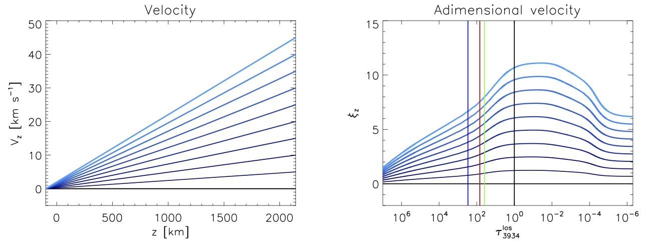
Figure 4.7: Amplification of the line anisotropy ($\rm{w_{line}}=\sqrt{2}\bar{J}^{2}_{0}/\bar{J}^{2}_{0}$) due to vertical velocity gradients. Upper left panel: linear velocity fields versus height, with velocity gradients going from $0$ (darker lines) to $20\,\rm{m\cdot s^{-1}\,km^{-1}}$ (light blue lines) in steps of $2.23\,\rm{m\cdot s^{-1}\,km^{-1}}$. Upper right panel: corresponding adimensional velocity fields ($\xi_{z}$) for a FALC temperature stratification and a constant microturbulent velocity of $3.5\,\rm{km\,s^{-1}}$. The horizontal axis is in units of the K-line optical depth along the line of sight (los). The vertical lines mark the position of $\tau^{\rm{los}}_{\nu_{0}}=1$ for the transitions $8498$ Å (blue), $8542$ Å (green), $8662$ Å (red) and the K line (black). Remaining panels: corresponding line anisotropy factors plotted against $\tau^{\rm{los}}_{\nu_{0}}$ for each line.

4.4.2 The impact of the emergent radiation on the polarization.

For investigating the effect of vertical velocity fields on the emergent fractional polarization profiles we perform the following numerical experiments. First, we impose velocity gradients with the same absolute value but opposite signs (top left panel of Fig. 4.8). The resulting emergent $Q/I$ profiles (remaining left panels of Fig. 4.8) are magnified by a significant factor ($>2$ for all the transitions) with respect to the static case (black dotted line). The linear polarization profiles have the same amplitude, independently of the sign of the velocity gradient. Another remarkable feature is the asymmetry of the profiles, having a higher blue wing in those cases in which the velocity gradient is positive and a higher red wing when the velocity gradient is negative, independently of the velocity sign. Note also that the $Q/I$ profile is shifted in frequency due to the relative velocity between the plasma and the observer.

As a second experiment, we consider different velocity fields with increasing gradients (right upper panel in Fig. 4.8). In the ensuing $Q/I$ profiles we see that the larger the velocity gradient, the larger the frequency shift of the emergent profiles and the larger the amplitude. In all transitions, one of the lateral lobes of the signal remains almost constant. Thus, what really changes is the central part of the profiles, being a “valley” in the $\lambda 8498$ line and a “peak” in the other two transitions. To quantify these variations, we define $(Q/I)_{\mathrm{pp}}$ (peak-to-peak amplitude of $Q/I$) as the difference between the lowest and the highest value of the emergent $Q/I$ signal, which is also a measure of its contrast. Note that, as expected from the first experiment, $(Q/I)_{\mathrm{pp}}$ depends only on the absolute value of the gradient. Figure 4.9 summarizes these results.

The sensitivity of the linear polarization to the velocity gradient can be measured approximately as commented in Sec. 4.3.1, using a parameter $\alpha=\Delta\nu_{D}/w$ that accounts for the difference in width of the absorption profile with respect to the emergent intensity profile. If $\alpha\thicksim 1$ in the main formation region, small adimensional velocities will produce large changes in shape; if $\alpha\ll 1$, much larger $\xi_{z}$ values are needed for the same effect. In the case of the IR triplet lines, $\alpha\thicksim 0.355$ in the formation region of $\lambda 8498$ and around $0.29$ and $0.285$ in the formation region of $\lambda 8542$ and $\lambda 8662$ (having wider profiles), respectively. Then, the former is more sensitive to velocity variations in its formation region (Fig. 4.9). Finally, the K line has $\alpha\,(\tau^{\rm{los}}_{\nu_{0}}=1)\thicksim 0.015$, a low value due to its wider spectral wings.

The enhancement of the polarization signals are a consequence of the increase in the anisotropy. Therefore, since this increase is produced by the presence of velocity fields, the polarization signals of the Ca ii IR triplet are sensitive also to the dynamic state of the chromosphere.

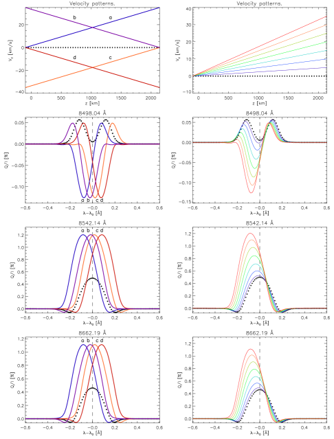
Figure 4.8: Left panels: calculation at $\mu=0.1$ of the emergent $Q/I$ polarization signals of the Ca ii IR triplet when four different choices for the vertical velocity gradients are imposed. Positive velocities imply upflowing plasma. Gradient “a”/“b” simulates an atmosphere where the plasma is entirely moving towards the observer increasing/decreasing linearly the velocity along the outgoing z axis. Gradients “c” and “d” are the same for plasma moving away from the observer. The black dotted line is the solution for the static reference case. Each curve is computed on the converged solution of the multilevel NLTE problem described in Sec. 4.2. Right panels: same calculations than in the left-hand panels, but with different velocity gradient values varying from $0$ to $16.3\,\rm{m\,s^{-1}\,km^{-1}}$ in steps of $2.3\,\rm{m\,s^{-1}\,km^{-1}}$ (see top right panel). These results show that the polarization signals are increased and shifted with respect to the static case depending only on the absolute value of the vertical velocity field gradient and independently of the sign of the velocity field.

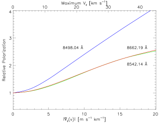
Figure 4.9: $(Q/I)_{\mathrm{pp}}$ normalized to the static case solution versus the velocity gradient (bottom axis) and the maximum absolute velocity (top axis) for linear velocity fields appearing in Fig. 4.8. The results are invariant under velocity sign changes. The transition $\lambda 8498$ is more sensitive to velocity variations due to its larger value of $\alpha=\Delta\nu_{D}/w$.

4.4.3 Variations on the atomic alignment due to velocity gradients.

In order to get physical insight on the formation of the emergent polarization profiles, we use an analytical approximation. Following Trujillo Bueno (2003b), the emergent fractional linear polarization for a strong line at the central wavelength can be approximated with (see Sec. 2.4.2):

$$\frac{Q}{I}\thickapprox\frac{3}{2\sqrt{2}}(1-\mu^{2})\left[{\sc}w^{(2)}_{J_{u}J_{\ell}}\cdot\sigma^{2}_{0}(J_{u})-{\sc}w^{(2)}_{J_{\ell}J_{u}}\cdot\sigma^{2}_{0}(J_{\ell})\right].$$ (4.13)

The symbols ${\sc}w^{(2)}_{JJ^{\prime}}$ are numerical coefficients already introduced in Sec. 4.2. The quantities $\sigma^{2}_{0}(J_{u})$ and $\sigma^{2}_{0}(J_{\ell})$ are the fractional alignment coefficients ($\sigma^{2}_{0}=\rho^{2}_{0}/\rho^{0}_{0}$) evaluated at $\tau^{\rm{los}}_{\nu}=1$ for the upper and lower level of the transition, respectively. This is the generalization of the Eddington-Barbier (EB) aproximation to the scattering polarization and establishes that changes in linear polarization (for a static case) are induced by changes in the atomic aligment of the energy levels.

Our calculations show that vertical velocity fields with moderate gradients ($\lesssim 10\,\rm{m\,s^{-1}km^{-1}}$ in a linear velocity field, as the ones shown in the figures) do indeed produce variations in the fractional alignment, which are small for $|\sigma^{2}_{0}(J_{u})|$ and significant for $|\sigma^{2}_{0}(J_{\ell})|$ (see Fig. 4.10). The lower level alignment is the main driver of the changes produced in the analyzed $Q/I$ signals. This is strictly true for the $\lambda 8662$ line, whose upper level with $J=1/2$ cannot be aligned (zero-field dichroism polarization). In the other transitions of the triplet, a certain influence of the upper level alignment becomes notable only for large gradients. The reason of this behavior is that the strong K transition is dictating the common upper level-5 alignment (Fig. 4.1). In fact, $\sigma^{2}_{0}(J_{5})$ is driven by the K line anisotropy which, at cromospheric heights, is almost unaffected for the considered velocity gradients, as we discussed in Sec. 4.4.1 (Fig. 4.7). Thus, the strong H and K lines feed population to the upper levels and the K line controls the alignment of the ${}^{2}P_{3/2}$ level (see Fig. 1), while the polarization signals of the IR triplet change with velocity fields affecting $\sigma^{2}_{0}(J_{\ell})$ (through the anisotropy enhancement).

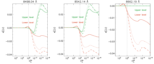
Figure 4.10: Behaviour of the fractional alignments $\sigma^{2}_{0}(J_{u})$ (green) and $\sigma^{2}_{0}(J_{l})$ (red) of each Ca ii IR triplet transition for three of the velocity fields shown in Fig. 4.8. The solid lines correspond to the reference static case. The dotted lines correspond to the case with maximum velocity $15\,\rm{km\,s^{-1}}$. The dashed lines are associated with the case with maximum velocity $30\,\rm{km\,s^{-1}}$. The horizontal axis is the line center optical depth for each value of the velocity gradient. The vertical dotted line marks the height where $\tau^{\rm{los}}_{\nu_{0}}=1.$

To illustrate the well-known link between the alignment and the anisotropy we can follow the next reasoning. For the Ca ii model atom we deal with in this work, it is posible to derive a simple analytic expression that relates the anisotropy and the alignments of the $\lambda 8542$ transition. Making use of Eqs. (A.12) and (A.13) and neglecting second order terms and collisions, we find that:

$${2}\sigma^{2}_{0}(J_{5})-{\sqrt{7}}\sigma^{2}_{0}(J_{3})\simeq{\sc w}_{line}(3\rightarrow 5).$$ (4.14)

As before, we can roughly assume that $\sigma^{2}_{0}(J_{5})\thicksim\rm{constant}$ in the chromosphere because it is controlled by the K line. Then, Eq. (4.14) suggests that, if the radiation anisotropy increases at those heights, an amplification of $|\sigma^{2}_{0}(J_{3})|$ occurs (note that $\sigma^{2}_{0}(J_{3})$ is negative for these lines). A more aligned atomic population produces a more intense scattering polarization signal.

4.5 Conclusions

When vertical velocity gradients exist, the polarization profiles are always shifted in wavelength, asymmetrized and enhanced in amplitude with respect to the constant velocity case. The reason is that increments in the absolute value of the velocity gradient increase the source function (Doppler brightening) and enhance the anisotropy of the radiation field (Secs. 4.3 and 4.4), that in turn modify the fractional alignment (Sec. 4.4.3) and amplify the scattering polarization profiles (Sec. 4.4.2).

For this very reason, all calculations assuming static models in the formation region might underestimate the scattering polarization amplitudes and not capture the right shape of the profiles. In particular, it must be taken into account that the Ca ii IR triplet lines form under non-LTE conditions in chromospheric regions, where velocity gradient may be significantly large due to the upward propagation of waves in a vertically stratified atmosphere (e.g., Carlsson & Stein, 1997). Probably, in photospheric and transition region lines the effect of velocities on polarization can be safely neglected (they will be predominantly amplified by temperature gradients as discussed in Sec. 4.3.3), but not necessarily in the chromosphere. In our study we see that the $\lambda 8498$ line is more sensitive to macroscopic motions in the low-chromosphere, while the $\lambda 8542$ and $\lambda 8662$ lines are especially amplified when strong velocity gradients are found at heights around $1.5\,\rm{Mm}$ and higher in our model.

At the light of these results, it is obvious that the effect of the velocity might be of relevance for measuring chromospheric magnetic fields. In particular, the described mechanism might turn out to be important for the correct interpretation of polarization signals in the Sun with the Hanle effect. Given that weak chromospheric magnetic fields are inferred with the Hanle effect using the difference between the observed linear polarization signal and the signal that would be produced in the absence of a magnetic field, it is relevant to compute the reference no-magnetic signal including velocities.

The polarization amplification mechanism that we have discussed in this chapter is not limited to plane-parallel atmospheres, although its effect is surely more important in plane-parallel atmospheres than in three-dimensional ones. The reason is that i) gradients in a three-dimensional atmosphere are expected to be weaker given the increased degrees of freedom and ii) significant variations in velocity direction along the medium mix the spectral contribution of different layers to the radiative transfer and broaden the emergent profiles, masking the Doppler features.

Chapter 5 Scattering Polarization of the Ca ii IR triplet in Hydrodynamical Models

In Chapter 4 we showed that velocity gradients can significantly affect the scattering polarization of the IR triplet of Ca ii. Our arguments were based on radiative transfer (RT) calculations in a semi-empirical model of the solar atmosphere, after introducing ad hoc velocity gradients and comparing the computed $\mathrm{Q/I}$ profiles with those corresponding to the static case. Given the diagnostic potential of the Ca ii IR triplet for exploring the magnetism of the solar chromosphere (e.g., Manso Sainz & Trujillo Bueno, 2010; De la Cruz Rodríguez et al., 2012), and the fact that the region where such chromospheric lines originate may be affected by vigorous and repetitive shock waves (e.g., Carlsson & Stein, 1997), it is necessary to investigate this RT problem using dynamical, time-dependent atmospheric models of the solar chromosphere.

In this chapter, we show the results of such investigation. Thus, we analyze the emergent linear polarization profiles of the Ca ii infrared triplet after solving the RT problem of scattering polarization in time-dependent hydrodynamical models of the solar chromosphere, taking into account the effect of the plasma macroscopic velocity on the atomic level polarization. We discuss the influence that the velocity and temperature shocks in the considered chromospheric models have on the temporal evolution of the scattering polarization signals of the Ca ii infrared lines, as well as on the temporally averaged profiles. We also study the effect of the integration time, the microturbulent velocity and the photospheric dynamical conditions, and discuss the feasibility of observing the temporal variation of the scattering polarization profiles with large-aperture telescopes. Finally, we explore the possibility of using the differential Hanle effect in the IR triplet of Ca ii to infer magnetic fields in dynamic situations. This chapter is adapted from Carlin et al. (2013).

5.1 Description of the problem and the resolution procedure.

We have carried out RT calculations of the scattering polarization in the Ca ii infrared (IR) triplet. The polarization is produced by the atomic level polarization induced by anisotropic radiation pumping in the hydrodynamical (HD) models of solar chromospheric dynamics obtained by Carlsson & Stein (1997, 2002).

We used two time series of snapshots from the above-mentioned radiation HD simulations, each one lasting about 3600 s and showing the upward propagation of acoustic wave trains growing in amplitude with height until they eventually produce shocks. The first one corresponds to a relatively strong photospheric disturbance showing well-developed cool phases and pronounced hot zones at chromospheric heights (see Carlsson & Stein, 1997, which will be referred to as the strongly dynamic case). The second simulation corresponds to a less intense photospheric disturbance (the weakly dynamic case given by Carlsson & Stein, 2002). Thus, the thermodynamical evolution of the atmosphere (including the chromosphere and the transition region) is driven by the bottom boundary condition that is imposed on the velocity. This realistic boundary condition is extracted from the measured Doppler shifts in the Fe i line at $3966.8$ Å. Our description focuses mainly on the strongly dynamic case, but in Sec. 5.3.5 we compare the results with those corresponding to the weakly dynamic case.

To characterize the simulations we can use the following quantities. In terms of the velocity gradients, and using units related to a representative scale height $\mathcal{H}=275\,\rm{km}$, the temporal average of the maximum velocity gradient along the atmosphere is $40\,\rm{km\,s^{-1}}$ per scale height (or $145\,\rm{m\,s^{-1}km^{-1}}$) in the strongly dynamic case and $13\,\rm{km\,s^{-1}}$ per scale height (or $47\,\rm{m\,s^{-1}km^{-1}}$) in the weakly dynamic case. Likewise, the temporal average of the minimum of temperature in the atmosphere is $\rm{3976\,K}$ in the strongly dynamic case, and $\rm{4292\,K}$ in the weakly dynamic case.

At each time step of the HD simulation under consideration we use the corresponding one-dimensional stratifications of the vertical velocity, temperature and density to compute the emergent $\rm{I(\lambda)}$ and $\rm{Q(\lambda)}$ profiles through the application of the multilevel radiative transfer code of Manso Sainz & Trujillo Bueno (2003b, 2010), after the generalization to the non-static case described in Sec. 3.1.2. Specifically, we have jointly solved the radiative transfer (RT) equations for the Stokes I and Q parameters and the statistical equilibrium equations (SEEs) for the atomic populations of each energy level and the population imbalances among its magnetic energy sublevels (equivalently, the multipolar tensor components of the atomic density matrix, $\rm{\rho^{K}_{0}(J_{i})}$, with $\rm{J_{i}}$ the angular momentum of each level i). This is the NLTE radiative transfer problem of the second kind (see Sections 7.2 and 7.13 in Landi Degl’Innocenti & Landolfi, 2004). Once the self-consistent solution of such equations is found at each height in the atmospheric model under consideration, we compute the coefficients of the emission vector and of the propagation matrix (see Sec. 4.2.2) and solve the RT equations for a line of sight (LOS) with $\mu=0.1$, where $\mu$ is the cosine of the heliocentric angle. This LOS has been chosen in order to simulate a close to the limb observation, such as that shown in Figure 13 of Stenflo et al. (2000). To account for macroscopic motions, we have introduced the Doppler effect in the calculation of the absorption and emission profiles for each wavelength and ray direction (Sec. 3.1.2). The influence of the Doppler effect on the SEE appears directly because the radiative rates depend on the radiation field tensor components. Likewise, the RTE is affected because the Doppler effect modifies the elements of the propagation matrix and of the emission vector.

Given that the computations reported here are carried out in plane-parallel atmospheric models, it is necessary to introduce a microturbulent velocity, which accounts for the Doppler shifts (inducing an effective line broadening) by moving fluid elements below the resolution element. In order to estimate a suitable value (assumed constant with height), we have calculated the emergent intensities at disk center and compared them with those of the solar Kitt Peak FTS Spectral Atlas (Kurucz et al., 1984). A good agreement is obtained with $3.5$ km s^-1.

5.2 Description and characterization of the results.

A standard Fourier analysis of the atmosphere model shows that it acts as a passband filter for the multifrequency sound waves generated in the lower boundary. The result is that the predominating periods at chromospheric heights and higher are around three minutes (Carlsson & Stein, 1997). For practical reasons, we divided the temporal evolution in three-minute intervals so that the beginning of each interval coincides with the moment in which the shock front in temperature and velocity is the sharpest in each interval (vertical lines in figures with temporal axis, like Figure 5.1). Given the power of the three-minute waves, this division turns out to be “natural” and can be used to mark the most interesting events we see in the emergent polarization.

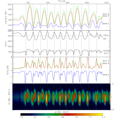
Figure 5.1: Top row: time evolution of the atmospheric heights where $\tau^{\rm los}_{\nu_{0}}=1$ for the three Ca ii IR transitions. The dotted vertical lines are located at the local minimum of the $\tau^{\rm los}_{8452}=1$ curve, and we use them to indicate the beginning and the end of each “three-minute” period. Second row: time evolution of the temperature value and atmospheric height of the temperature minimum. Third row: time evolution of the polarization contrast ($\rm{\max(Q/I)-\min(Q/I)}$) for the three lines of the Ca ii IR triplet. The polarization amplitude of the ${\lambda}8498$ line has been multiplied by -5 to show the results for the three lines on the same scale. Note that, by definition, the line contrast is always positive. However, we added an artificial negative sign to the 8498 Å line contrast values in this figure to illustrate that its polarization amplitudes are predominantly negative. Bottom row: time evolution of the calculated $\rm{Q(\lambda)/I(\lambda)}$ fractional linear polarization profile of the ${\lambda}8542$ line.

Inside each three-minutes cycle we distinguish between compression and expansion phases. They can be easily identified following the height at which $\tau^{\rm los}_{\nu_{0}}=1$, i.e., where the optical depth at line center ($\nu_{0}$) along the LOS equals unity (upper panel of Figure 5.1). This quantity is a good marker of the shock fronts when they cross heights between $1$ and $2$ Mm. It is because the steep changes in opacity inside the shocks forces the $\tau=1$ region to remain comprised within them. The line transitions at $8542$ Å and $8662$ Å (green and red lines in the upper panel of Figure 5.1) follow a clearer periodic pattern because they form higher, where less frequency components of the velocity waves can arrive. Compression phases begin when plasma falls down from upper layers ($\tau^{\rm los}_{8542}=1$ and $\tau^{\rm los}_{8662}=1$ decrease in the top panel of Figure 5.1), while simultaneously a new upward propagating wave emerges amplified into the chromosphere. At the end of this stage a shock wave is completely developed and the $\tau^{\rm los}_{\nu_{0}}=1$ position is close to $\sim$1200 km for the three IR lines. The shock waves so created always start in such region between 1 and 1.5 Mm. After that, during what we term expansion phase (heights for $\tau^{\rm los}_{8542}=1$ and $\tau^{\rm los}_{8662}=1$ arising in top panel of Figure 5.1), the shock fronts travel upward increasing the plasma velocities as they encounter lower densities.

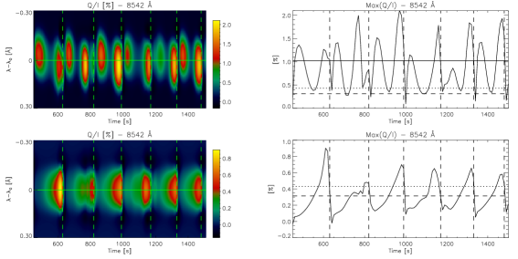
Figure 5.2: Temporal evolution of $\rm{Q(\lambda)/I(\lambda)}$ (left column panels) and of the ${\rm{Max}}(Q/I)$ peak amplitude (right column panels) during 1040 s (17 minutes) for the 8542 Å transition. Upper panels: results taking into account the effect of the velocity gradients. Lower panels: results assuming no macroscopic velocities while calculating the density-matrix elements. The vertical lines indicate the beginning and the end of each three-minutes period. The horizontal lines in the right column panels show the temporally-averaged amplitudes ($\rm{\langle Q\rangle/\langle I\rangle}$) for three cases: RT in the strongly dynamic model including velocities (solid line); RT in the strongly dynamic model but setting $v=0$ (dashed lines); RT in the (static) semi-empirical FAL-C model (dotted lines).

Figure 5.1 also shows the time evolution of other quantities during the first $2000$ s after the initial transient. In the second row, the location and value of the temperature minimum are displayed, showing a clear correspondence with expansion and contraction phases. In the third row, we show the ensuing variation of $\rm{(Q/I)_{pp}}$, defined as the peak-to-peak difference of the Q/I profile for each spectral line. It is a measure of the linear polarization signal contrast that was used in Chapter 4 to characterize the polarization amplitude and discriminate their variations with respect to static cases. In each cycle we see an amplification of $\rm{(Q/I)_{pp}}$ occurring at expansion phases and an usually larger amplification during contraction phases. Finally, the time evolution of the emergent $\rm{Q(\lambda)/I(\lambda)}$ profile for the $8542$ Å line is illustrated in the lower panel (the vertical axis shows 0.6 Å around the rest wavelength of the line). Here, we observe two distinct areas showing amplifications inside each three-minute cycle. The first amplification is blueshifted, because it happens in an atmospheric expansion phase (plasma moving toward the observer). It is weaker than the second amplification, which is redshifted and occurs during the compression phase (plasma moving down in the atmosphere). This indicates that the compression phase is more efficient producing a polarization amplification than the expansion one. The reason is that during compression we have stronger velocity and temperature gradients along the main regions of formation. Following the results of Chapter 4, the larger the gradient, the larger the enhancement of the linear polarization signal. The behavior is similar in the other transitions.

There is a clear correspondence between the maximum value of the temperature minimum (hot-chromosphere time steps) and the largest peaks of the $\rm{(Q/I)_{pp}}$ signal, taking place just before the maximum contraction (dotted vertical lines). As the atmosphere is compressed, the temperature increases at chromospheric heights and the resulting gradient of the source function produces an increase of the radiation field anisotropy in the upper layers. This directly leads to an enhanced emergent linear polarization signal. On the contrary, in cold-chromosphere models the expansion reaches its maximum and $\rm{(Q/I)_{pp}}$ is near its minimum value.

Even in such complex situations, we still witness the already known effects of amplification (with respect to the static case), frequency shift and asymmetry in the linear polarization profiles due to dynamics. All of them have been already explained in Chapter 4, using the semi-empirical FAL-C model of Fontenla et al. (1993) with ad-hoc velocity stratifications. The enhancement is produced as a consequence of the velocity gradients and subsequent anisotropy enhancements. However, some differences exist from the experiments in semi-empirical models and the calculations presented in this chapter. First, the velocity stratification in the HD models is, in general, non-monotonic and with a non-constant variation with height. Second, the maximum velocity gradients are located at shocks, with amplitudes that reach tens or even hundreds of meters per second per kilometer (as a comparison, in Chapter 4 we dealt with velocity gradients between 0 and 20 m s^-1 km^-1). Third, as commented before, we have shocks in temperature that produce larger source function gradients and additional enhancement of the radiation anisotropy and of the linear polarization. Finally, these variations are usually concentrated in the formation regions of the triplet lines. All these mechanisms act together and enhance the linear polarization of the emergent radiation with amplification factors up to $\sim 10$ (in the $8498$ Åline) and $\sim 7$ (in the $8542$ Å and $8662$ Å lines), for the instantaneous values of the $\rm{Q/I}$ amplitudes with respect to the static FAL-C case. However, if we consider temporal averages of the emergent Stokes profiles during long periods, we get amplification factors of about a factor of two (time-averaged Q/I amplitudes reach $\sim 1\,\%$ for 8542 Å and 8662 Å lines).

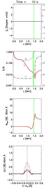
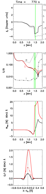
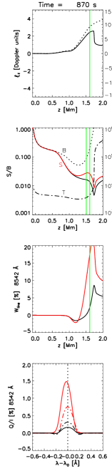
Figure 5.3: The effect of the velocity gradient for the time steps 10 s. (left column, a ‘quiet’ situation), 770 s. (middle column, a compression stage) and 870 s. (right column, an expansion phase) in the strongly dynamic hydrodynamical simulation. First row (from top): macroscopic vertical velocity (dotted line) and adimensional vertical velocity $\xi_{z}$ (solid line) versus height.Second row (from top): temperature (dashed line), Planck function (dotted line), source function for the zero velocity approximation (solid black line) and source function allowing the influence of the model’s velocity gradients (red solid line). Third row (from top): line anisotropy factor (Equation 4.4) calculated for each of the above-mentioned cases; neglecting the effect of the velocity gradients (black solid line) or allowing it (red solid lines). Fourth row (from top): emergent $\rm{Q/I}$ profiles versus wavelength (respect to the line center), with the same color code as in previous panels. The dashed lines here are the time averages over the entire simulation for each case (with or without velocities). The green lines mark the instantaneous positions of $\tau^{\rm los}_{\nu_{0}}=1$ and $\tau^{\rm los}_{\nu_{0}}=2$.

Summarizing, the temporal evolution of the polarization is driven by the temperature and velocity stratifications, that in turn are a result of the dynamical conditions set in the photosphere.

5.3 Analysis and discussion of results.

5.3.1 The effect of the velocity.

A way of visualizing the effect of vertical velocity gradients on the emergent scattering polarization is to compare the evolution of the polarization profiles corresponding to both the static and non-static case. In the absence of velocities (lower row of Figure 5.2), the maximum of the $\rm{Q/I}$ profiles is always located at $\lambda=\lambda_{0}$ (i.e., line center), and its temporal evolution presents a sawtooth shape. When the effect of velocities is included in the calculations (upper row of Figure 5.2), the maximum of the $\rm{Q/I}$ signal is no longer located at the central wavelength and its temporal evolution assumes a different shape with two peaks every three-minute period (upper right panel). These wavelength and amplitude modulations are produced by the Doppler effect of the velocity gradients.

It is interesting to compare the mean $\rm{Q/I}$ amplitudes obtained in the HD models with the one calculated in the FAL-C model. They differ notably (see horizontal lines in right panels of Figure 5.2). In the $8542$ Å transition we have mean values around $1\%$, $0.31\%$ and $0.42\%$ for the HD models with velocities, the HD models at rest and static FALC models, respectively. The results of these figures have been obtained using an integration time of $1040$ s ($\backsim 17$ minutes), the duration of the temporal interval shown in Figure 5.2. Neglecting the effect of the velocity gradients in the HD models, we see that the resulting temporally averaged scattering polarization signals (which include the impact of the temperature and density shocks) are similar to the $\rm{Q/I}$ profiles computed in the static FAL-C semi-empirical model.

5.3.2 The combined effect of velocity and temperature on the linear polarization.

In Figure 5.3 we display some relevant magnitudes for three different situations in the simulation. The first column corresponds to a quiet time step, with no shocks, zero velocity and without any kind of amplifications (it is the initial transient phase). The central column shows a phase of compression, in which shocks are important. Finally, the last column displays an expansion phase, in which the atmosphere is expanded and the shocks are already travelling over the transition region. Furthermore, we distinguish between the solutions when motions are taken into account (red lines) and the solutions obtained allowing shocks in all magnitudes but artificially setting the velocity to zero (black lines).

The normalized velocity $\rm{\xi_{z}=(\nu_{0}/c)v_{z}/\Delta\nu_{D}}$, with $\rm{\Delta\nu_{D}}$ being the Doppler width of the absorption profiles (which depends on the temperature), c the speed of light and $\rm{v_{z}}$ the vertical velocity, is the quantity that controls the importance of the atmospheric motions in relation with the radiation anisotropy and the scattering polarization (see Sec. 4.3.3). Note that this quantity considers the combined effect of velocity and temperature. In the HD atmosphere models, $\rm{\xi_{z}}$ (solid lines in upper panels of Figure 5.3) is only significant in the formation region of the IR triplet lines ($\tau^{\rm los}_{\nu_{0}}\sim 1$ region with high velocity gradients, and not very high temperatures). Although shock waves increase the chromospheric temperature, the effect of the velocity gradients is predominant. The contrary occurs over the transition region, where the thermal line width is much larger than the Doppler shifts.

The expansion and contraction can be identified also in quantities such as the intensity source function and the Planck function (second row in Figure 5.3). During contraction phases (middle column panels), high temperatures produce a more efficient population pumping toward upper levels, increasing the emissivity and, consequently, the source function. Additionally, during contraction the temperature shock occurs in optically thick and denser layers (deeper layers below $\tau^{\rm los}_{\nu_{0}}=1$), forcing the source function gradient to increase with respect to the static case at those heights. Note how in this last case the source function rises as a whole because of the warming (compare the source function in the middle panel, the black solid line that has been obtained neglecting velocities, with the non-dynamic source function in the left column). If the macroscopic velocity is now considered, we additionally get a jump in the source function (red lines in middle column of Figure 5.3) caused by the velocity shock that is developed in this contraction phase. This behavior is accompanied by a significant Doppler-induced anisotropy enhancement that amplifies the linear polarization, as shown in the corresponding lower panels of the same figure.

In the expansion phases, the shock waves move upward and the chromosphere becomes cooler. This induces a lower source function and smaller polarization amplitudes (as compared with the contraction phase). Otherwise, as the density of scatterers is now lower around the shock (because it moved upward to regions with $\tau^{\rm los}_{\nu_{0}}<1$), the temperature gradients have smaller effects on the polarization profiles than during the contraction phases. In this expansion time step, the black solid line representing the static source function is similar to the non-dynamic source function of the left column. However, once the motions are introduced, and despite of the fact that the shocks have already reached upper chromospheric layers, the remanent velocity field has still a sizable gradient that enhances the source function (Doppler brightening effect).

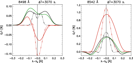
Figure 5.4: Fractional linear polarization profiles of the 8498 Å and 8542 Å lines after temporally averaging the Stokes I and Q profiles during 3070 seconds (51 minutes). These $\rm{\langle Q\rangle/\langle I\rangle}$ profiles may be considered to emulate what can be actually observed with today’s solar telescopes. Black solid profiles: static case with $v_{\rm{micro}}=3.5\,\rm{km\,s^{-1}}$. Red solid profiles: strongly dynamic case taking into account the effect of the velocity gradients and assuming $v_{\rm{micro}}=3.5\,\rm{km\,s^{-1}}$. Black dashed profiles: strongly dynamic case neglecting the effect of the velocity gradients and assuming $v_{\rm{micro}}=0$. Red dashed profiles: strongly dynamic case taking into account the effect of the velocity gradients and assuming $v_{\rm{micro}}=0$. The green solid lines show the temporally averaged profiles obtained after applying the velocity free approximation (VFA) with $v_{\rm{micro}}=3.5\,\rm{km\,s^{-1}}$ (i.e., neglecting the Doppler shifts of the macroscopic velocities when computing the density matrix elements, but taking them into account when calculating the emergent Stokes profiles).

5.3.3 Averaged values of the polarization profiles.

In order to compute the average linear polarization signal that one would observe without any temporal resolution, we average Q and I (obtaining $\rm{\langle Q\rangle/\langle I\rangle}$) over $3070\,\rm{s}$ ($\approx 51$ minutes) for four different cases (Figure 5.4). We consider the cases with zero microturbulent velocity (dotted lines) and a constant microturbulent velocity of 3.5 km s^-1 (solid lines). For each case, we distinguish between the results switching off the velocity (black lines) and the results allowing for macroscopic velocity fields (red lines).

When macroscopic motions are considered, the polarization profiles become amplified asymmetrically. Furthermore, they are negative in the case of the 8498 Å transition and positive in the other two transitions. The asymmetry of the red profiles is a consequence of the fact that, during the averaging period, the dynamical situations in which the velocity gradient is negative (velocity field mostly decreasing with height) dominate over the situations with velocity gradients that are mostly positive. This predominance is not because the situations with negative velocity gradients are more frequent but because such situations are more efficient on amplifying the linear polarization and thus, their effect prevails. This happens during the compression phase because i) the velocity gradients are larger, ii) there is also a shock in temperature affecting the formation region and iii) the shock fronts are located just below the $\tau^{\rm los}_{\nu_{0}}=1$ height. The results are qualitatively the same independently of the microturbulent velocity value, but, when it is not considered, the amplification of $\rm{(Q/I)_{pp}}$ is larger and the profiles are narrower.

If we decrease the averaging interval to $9$ minutes, we obtain profiles that are essentially similar to the ones obtained by averaging during $51$ minutes (showed in Figure 5.4). If we integrate less than that, significant variations appear in the shape and amplitude of the emergent profiles. This indicates that, concerning the linear polarization, there is still reliable dynamic information contained in a time interval corresponding to a few three-minute cycles.

5.3.4 The velocity free approximation.

An approximation that is sometimes applied to solve radiative transfer problems in dynamical atmospheres (either taking into account the presence of atomic polarization or not) is the velocity free approximation (VFA). It is based on solving the SEE and RTE simultaneously but neglecting the effect of plasma motions. However, once they are consistently solved, such plasma motions are included in the synthesis of the emergent Stokes profiles (along $\mu=0.1$ in our case). Consequently, the density matrix elements are calculated as if plasma motions did not affect them, reducing the complexity and computational effort of the problem since a reduced frequency grid is used to compute the mean intensity and the anisotropy. The results of applying it to each time step of our HD evolution is the temporal average illustrated as the green line in Figure 5.4. This approximation is clearly not appropriate in our case, given that the profiles just become asymmetric (with respect to the static profiles) but without the amplification. The reason for this lack of amplification is that the anisotropy controlling the linear polarization is not correctly enhanced (see Chapter 4). On the other hand, the asymmetry is purely due to the asymmetric absorption with respect to the line center that motions produce along the ray under consideration. Hence, in order to obtain reliable results it is mandatory to include the effect of Doppler shifts in the whole set of equations, and we conclude that the VFA should not be applied.

5.3.5 The effect of photospheric dynamics.

Given that the small velocity fields appearing in the photosphere are amplified because of the exponential decrease in the density while the perturbations travel outward, the properties of the bottom boundary condition are determinant in the behavior of the emergent Stokes parameter of chromospheric lines. We compare the strongly dynamic case that forms the core of this chapter with the weakly dynamic case that has been already introduced in Sec. 5.2. Although the mean maximum velocity gradient is three times smaller in the weakly dynamic case and the averaged polarization amplitudes are also smaller than in the strongly dynamic one, we still find comparable or even slightly larger instantaneous $\rm{(Q/I)_{pp}}$ amplitudes (see Figure 5.5). The resulting averaged polarization profiles are qualitatively the same but they differ in amplitude (Figure 5.7). This is a reasonable result because in the weakly dynamic scenario the instantaneous velocity gradients are smaller in general. Differences are especially critical for the 8498 Å line, whose linear polarization profiles can be positive, but also adopt significant negative values at redder wavelengths (when velocity gradients are mainly positive with height) or at bluer wavelengths (when velocity gradients are mainly negative with height). This behavior produces cancellation effects with integration times larger than a three-minute period. Furthermore, the central depression produced in the 8498 Å average profile when the velocity is neglected in the strongly dynamic simulation (solid black line in left panel of Figure 5.7) do not appear in the average profile corresponding to the weakly dynamic case (dashed black line in the same panel) because of the differences in the instantaneous temperature stratifications. The sensitivity of this spectral line to the instantaneous photospheric perturbations and to the developed chromospheric shocks is larger than in the other two lines.

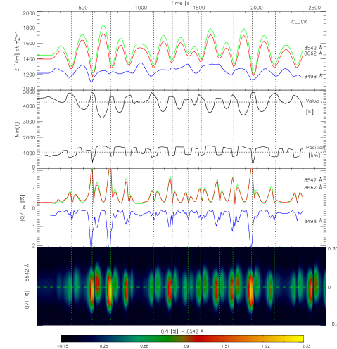
Figure 5.5: Same as Figure 5.1, but for the weakly dynamic case. Remember that the blue line amplitude has been multiplied by -5 for scale reasons.

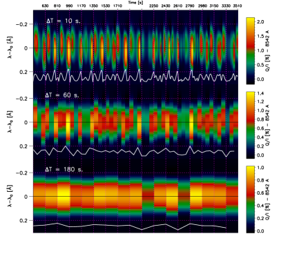
Figure 5.6: Temporal evolution of the emergent $8542\lambda$ $\rm{Q/I}$ profiles for different integration times. Wavelength is in the vertical axis. From top to bottom we have a 10, 60 and 180 s. temporal resolution, respectively. The white solid lines show the temporal evolution of $\rm{(Q/I)_{pp}}$ (i.e., the amplitude contrast at each time-step). Vertical dotted lines mark each three-minute period.

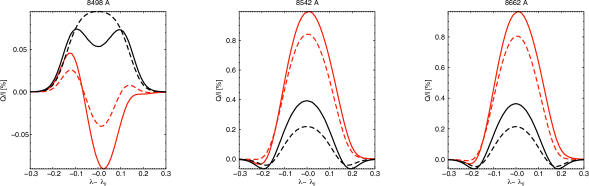
Figure 5.7: Comparison of the results in the strongly and weakly dynamic cases (see Sec. 5.3.5). All profiles are the resulting $\rm{\langle Q\rangle/\langle I\rangle}$ profiles obtained averaging Q and I during 15 minutes of the considered simulation. Solid lines: strongly dynamic case. Dashed lines: weakly dynamic case. Black lines: results allowing variations in all magnitudes but neglecting the velocity. Red lines: results including the velocity gradients.

5.3.6 The effect of the integration time.

In order to detect in the Sun the time evolution of the linear polarization signals, the observations must have enough time resolution, signal-to-noise ratio and spatial resolution. A sufficient spatial coherence is important to avoid cancellations of the contribution from different regions in the chromosphere evolving with different phases. If we consider the expected capabilities of the next generation of solar telescopes (like the European Solar Telescope, EST, or the Advanced Technology Solar Telescope, ATST), we can aim at observing the emergent Stokes profiles of Figure 5.6 with a 10 s cadence (upper panel). However, with the present telescopes and instrumentation, we are forced to integrate in time and/or space to detect the scattering polarization signals. If we degrade the temporal resolution of our results to an integration time of 1 minute (middle panel of Figure 5.6) and 3 minutes (lower panel of Figure 5.6) we clearly see that the time evolution becomes more difficult to detect. In the last case, the profiles are already so smoothed that the original features are completely lost, both in the spectral and temporal domains. The amplitude of the integrated signals are lower than in the original 10 s sequence by a factor of $2$ (see the color scales). However, integration during time intervals ${\sim}1$ minute could reveal the amplification/modulation effect if we capture spectro-polarimetric signals similar to the ones showed in the middle row panel.

Figure 5.8: Resulting $\rm{Q/I}$ profiles after averaging Q and I during $15$ minutes in the strongly dynamic simulation, using different values of $F$. $F$ is the scaling factor by which we have multiplied the modulus of the macroscopic velocity at each atmospheric height. The curves correspond to $F=0,\,0.1,\,0.2,\,0.5,\,0.7,\,0.9,\,1$, going from solid lines (static case and also $F=0.1$) to long dashed lines (fully dynamic case). The results for the 8662 Å line are very similar to the ones obtained for the 8542 Å line.

5.3.7 The effect of a decreasing velocity on the averaged profiles.

We also calculated what happens to the emergent averaged profiles in the strongly dynamic case (with $15$ minutes of integration, emulating an observation) when we gradually reduce the velocity field by a constant scaling factor $F$, keeping the rest of atmospheric magnitudes unperturbed (see Figure 5.8). As expected, we find that the polarization amplitudes decrease in proportion to $F$, from the original case, with $F=1$, towards the static case, with $F=0$. Note that the core of the 8498 Å line goes through zero for a certain $F$ value (near $F=0.6$). Thus, depending on the magnitude of the velocity gradients, its linear polarization amplitude will be positive or negative. This fact suggests an additional way to diagnose velocity gradients along the line-of-sight. However, it is important to keep in mind that this sensitivity also depends on the variations in density and temperature, as shown in Sec. 5.3.5.

Furthermore, the variation of the $\rm{Q/I}$ amplitudes is not linear with $F$. The change is small for small $F$, is larger for intermediate values of $F$, and again becomes smaller for the largest $F$, tending to saturation.

5.4 Considerations on the Hanle effect

For magnetic field diagnostics with the Hanle effect it is often necessary to know the zero-field polarization reference (e.g., Stenflo, 1994; Trujillo Bueno et al., 2004). That is what we have tried to do in previous sections, calculating and explaining the temporal evolution of the linear polarization profiles in chromospheric dynamic simulations. Ideally, this reference has to be computed under the same thermodynamical and dynamical conditions than in the real Sun but without magnetic field. As the Hanle effect often depolarizes the linear polarization signals, the difference between the observation and the zero-field calculation can be associated with a magnetic field by adjusting the magnetic field topology and intensity. The key point is that the reference amplitude must be as precise as possible. If it is imprecise, variations in the Stokes profiles can be associated with a magnetic field when they were really due to uncertainties in another magnitudes, like the temperature or the velocity field. Due to this reason, the fact that the solar chromosphere is a highly dynamic medium brings some complications for the use of the Hanle effect as a diagnostic tool.

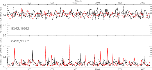
Figure 5.9: Black solid lines correspond to the strongly dynamic case. Red lines correspond to weakly dynamic case. Black dashed lines correspond to the strongly dynamic case but doing the calculations without microturbulent velocity. The line ratio $\varrho_{3}=(\rm{Q/I})^{8498}_{pp}/(\rm{Q/I})^{8542}_{pp}$ is not shown because it is very similar to $\varrho_{1}$ and because can be obtained from the other two ratios.

A strategy to avoid the above-mentioned problem is known as the line ratio technique. It consists in finding a pair of spectral lines whose thermodynamical behavior is identical but whose sensitivity to the magnetic field is different in some range of magnetic field intensity or inclinations (e.g., Stenflo et al., 1998; Manso Sainz et al., 2004). In that case, the ratio between the polarization amplitudes should only change due to variations in the magnetic field, thus allowing us to measure it after a suitable calibration. As shown by Manso Sainz & Trujillo Bueno (2010), the main magnetic sensitivity difference among the lines of the Ca II IR triplet is between the ${\lambda}8498$ line (which is sensitive to field strengths between 0.001 G and 10 G) and any of the ${\lambda}8662$ and ${\lambda}8542$ lines (which react mainly to sub-gauss magnetic fields and up to 10 G in the latter spectral line). Unfortunately, while the line-cores of the ${\lambda}8662$ and ${\lambda}8542$ lines originate in similar atmospheric layers, the ${\lambda}8498$ line-core originates at significantly deeper chromospheric layers (see e.g. Fig. 5.1). Nevertheless, we have found useful to plot in Figure 5.9 the time evolution of the following polarization line ratios:

$$\varrho_{1}=\frac{(\rm{Q/I})^{8498}_{pp}}{(\rm{Q/I})^{8662}_{pp}},$$ (5.1a)

$$\varrho_{2}=\frac{(\rm{Q/I})^{8542}_{pp}}{(\rm{Q/I})^{8662}_{pp}},$$ (5.1b)

where the super-index indicates the central wavelength of the transition in Å. These quantities were calculated for each simulation considered before (weakly and strongly dynamic cases). The more stable they are, the more useful they will be for inferring the magnetic field.

We obtain that , on average, $\bar{\varrho_{1}}=0.15\,\pm\,0.10$ and $\bar{\varrho_{1}}=0.16\,\pm\,0.14$ for the strongly and weakly dynamic cases, respectively (lower panel in Figure 5.9). The sudden shape variations (including maximum amplitudes passing through zero) of the 8498 Å line induce large instantaneous excursions on $\varrho_{1}$ . As expected, a more stable line ratio is obtained for the second pair of transitions, which are precisely the ones that originate at similar chromospheric heights. We find $\bar{\varrho_{2}}=1.06\,\pm\,0.11$ and $\bar{\varrho_{2}}=1.00\,\pm\,0.09$ for the strongly and weakly dynamic cases, respectively (upper panel in Figure 5.9). If we repeat the calculations setting to zero the microturbulent velocity in the strongly dynamic case we obtain $\bar{\varrho_{1}}=0.22\,\pm\,0.09$ and $\bar{\varrho_{2}}=0.97\,\pm\,0.12$ (dashed black lines in Figure 5.9). These results indicate that the $\bar{\varrho_{2}}$ line ratio shows a relatively stable behavior against variations of the velocity and temperature in the solar atmosphere. Consequently, in principle, $\varrho_{2}$ could be used as a suitable line ratio to estimate the magnetic field from spectropolarimetric observations of the ${\lambda}8662$ and ${\lambda}8542$ lines.

Regarding the sensitivity of these lines to the magnetic field and their applicability for the diagnostic of magnetic fields through the Hanle effect, several considerations have to be taken into account. First, the microturbulent velocity has a small influence on the averaged amplitudes and line ratios. Second, once the magnetic field is included in the calculations, the Hanle effect typically operates at the line center for static cases. However, in a dynamic situation there is not a preferred line center wavelength. As the maximum of the absorption and dispersion profiles occurs at different Doppler shifted wavelengths, the Hanle effect will operate in a small spectral region around the line core. Third, according to the static calculations by Manso Sainz & Trujillo Bueno (2010), for chromospheric magnetic fields stronger than $0.1$ G in the “quiet” Sun, the $\rm{Q/I}$ signal of the 8662 Å line is expected to be Hanle saturated. Thus, variations between $0.1$ and $10$ G could be measured with $\varrho_{2}$, being produced by changes in the linear polarization of the 8542 Å line. Unfortunately, the fluctuations we see in Figure 5.9 (exclusively due to the dynamics) have amplitudes of the same order of magnitude than those expected from the investigations of the Hanle effect in static model atmospheres (exclusively due to the magnetic field). More realistic results will be obtained when carrying out calculations of the Hanle effect of the Ca ii IR triplet in dynamical model atmospheres. In any case, it is clear that for exploiting the polarization of these lines, we need instruments of high polarimetric sensitivity.

5.5 Conclusions

The results presented in this chapter indicate that the vertical velocity gradients caused by the shock waves that take place at chromospheric heights in the HD models of Carlsson & Stein (1997; 2002) have a significant influence on the computed scattering polarization profiles of the Ca ii IR triplet. They show changes in the shape of the $\rm{Q/I}$ profiles of the three IR lines and clear enhancements in their amplitudes, as well as changes in the sign of the $\rm{Q/I}$ signal of the ${\lambda}8498$ line. Such modifications with respect to the static case are evident, not only in the temporally resolved $\rm{Q/I}$ profiles (e.g., see Figure 5.2), but also in the temporally averaged $\rm{\langle Q\rangle/\langle I\rangle}$ profiles (e.g., see Figure 5.4). This is true even with moderate macroscopic plasma velocities, simply due to the presence of strong vertical velocity gradients like the ones produced by shock waves. This explains why the above-mentioned modifications of the scattering polarization profiles of the Ca ii IR triplet are present also in the weakly dynamic simulation of Carlsson & Stein (2002).

Our investigation points out that the development of diagnostic methods based on the Hanle effect in the Ca ii IR triplet should take into account that the dynamical conditions of the solar chromosphere can have a significant impact on the emergent scattering polarization signals. This complication could be alleviated with the application of line ratio techniques. In Sec. 5.4 we have concluded that the ratio between the polarization amplitudes of the ${\lambda}8542$ and ${\lambda}8662$ transitions would be the best line-ratio choice. However, even in the absence of magnetic fields, the small fluctuations we see in the calculated values of such dynamic line ratios could be confused with the presence of magnetic fields in the range between $0.1$ and $10$ G. Further work is necessary to clarify this point.

In any case, the fact that realistic macroscopic velocity gradients may have a significant impact on the scattering polarization profiles of the Ca ii IR triplet is interesting for the diagnostic of the solar chromosphere. On the one hand, it provides a new observable for probing the dynamical conditions of the solar chromosphere (e.g., by confronting observed Stokes profiles with those computed in dynamical models). On the other hand, the exploration of the magnetism of the quiet solar chromosphere via the Hanle effect in the Ca ii IR triplet (either through the forward modeling approach or via foreseeable Stokes inversion approaches) would have to be accomplished without neglecting the possible effect of the atmospheric velocity gradients on the atomic level polarization.

Some points are still unanswered after this work. First, we need to investigate the sensitivity to the Hanle effect of the $\rm{Q/I}$ and $\rm{U/I}$ profiles of the Ca ii IR triplet using magnetized and dynamical atmospheric models. Second, we have to investigate whether our one-dimensional RT results remain valid after considering realistic three-dimensional models, such as those resulting from magneto-hydrodynamical simulations (e.g. Wedemeyer et al., 2004; Leenaarts et al., 2009b).

Finally, we mention that these results could be potentially interesting in other astrophysical contexts. For instance, the mechanism of polarization enhancement due to the presence of shocks might well be the explanation for the changing amplitudes of the linear polarization signals reported in variable pulsating Mira stars (Fabas et al., 2011).

Chapter 6 Synthesis of Stokes profiles in a 3D MHD atmospheric model.

In previous chapters we studied the basic effects that the temperature and the velocity structure of solar models atmospheres have on the synthetized scattering polarization profiles of the Caii IR triplet. Now we shall consider the action of the magnetic field as well, trying to obtain information about the influence that the dynamical state of the atmosphere can have on the diagnosis of cromospheric magnetic fields. To this end, we present the results of solving the NLTE RT problem of the second kind in a 3D solar atmosphere model obtained from a state-of-the-art magneto-hydrodynamical (MHD) simulation. The investigation focuses on the forward scattering geometry and the linear polarization signals produced by Hanle effect. To obtain the NLTE solutions we applied the 1.5D approach with the correct 3D populations supplied by the model at each point.

In this chapter we will study the spatial distribution and filling factor of the linear polarization signals affected by the dynamic, temperature and magnetic fields in a simulated quiet Sun. One of the aims is to identify the circumstances leading to miss the dynamic amplifications in the observational linear polarization signals. Are we actually missing them? Such effects, explained in previous chapters, have not been clearly captured by the telescopes so far and we want to know why. Furthermore, we will investigate the spatial patterns that the magnetic field and the temperature stratification create in the scattering polarization maps as well as how we could use them for diagnosis purposes. As an exercise, we will try to infer the magnetic field topology from the synthetic maps using the Hanle and Zeeman signals. Finally, we will dedicate a section to evaluate some spectropolarimetric quantities and observational strategies applied to signal detection under the physical situation of our models.

6.1 Description of the MHD model and the RT calculations.

The atmospheric model used to perform the spectral synthesis correspond to a snapshot of a radiation MHD simulation of the solar atmosphere computed by Leenaarts et al. (2009a) with the Oslo Stagger Code (Hansteen et al., 2007). This code solves the set of MHD equations that describe the plasma motion together with the RTE. It employs an LTE equation of state and includes non-LTE radiative losses using a multi-group opacity method and thin radiative cooling in the corona and upper chromosphere. It includes thermal conduction along magnetic field lines. The model has $256\times 128\times 213$ grid points and a physical size of $16.6\times 8.3\times 5.3$ Mm. But, to our aims, we selected a volume with $5.85\times 5.98\times 4$ Mm and $91\times 93\times 191$ grid points. The snapshot has a mean magnetic field strength of $120$ G at $300$ Km, which is representative of the magnetization expected in the quiet regions of the solar photosphere (Trujillo Bueno et al., 2004).

The (first-kind) 3D RT calculations performed by the Oslo Stagger Code to obtain the snapshot atmospheric stratifications were done under complete redistribution in frequency for all the spectral lines. We used the solutions of the 3D RT problem for the Ca ii level populations as a guess to solve the scattering polarization problem. The electron density was computed assuming LTE ionization for all relevant species. Photoionization by hydrogen Lyman lines was not taken into account.

The hydrogen number density was not available in the supplied model and we had to compute it. To this end, we considered the stratifications of temperature, density and electron number density and we solved the chemical equilibrium and ionization equations for all the relevant atomic species, including hydrogen, as explained in Asensio Ramos (2004).

We then solved the full RT problem for the Stokes vector by treating each model column as an independent planeparallel atmosphere (1.5D approach), neglecting the effect of horizontal inhomogeneities. The technical details of the core calculations and the computer program developed for performing them are described in Chapter 3.

Finally, as done in previous chapters, we add a constant microturbulent velocity $\mathrm{v_{\mu}=3.5\,km\cdot s^{-1}}$ to fit the calculated average of the $\lambda 8542$ line intensity of the model with the emergent intensity provided by a solar atlas (Kurucz et al., 1984).

6.1.1 Pre-processing the models.

The selected data cube contains $8463$ columns (hereafter, columns or models). In order to decrease the computational load, we adaptatively truncated the colums in height. We estimated the column heights where $\tau^{8498}_{\mathrm{cont}}=10^{3}$ (setting the lower boundary position) and $\tau^{\mathrm{K\,line}}_{\nu_{0}}=10^{-4}$ (setting the upper boundary position). Thus, we could run the RT calculations with less grid points but without appreciable loss of accuracy in the obtention of the density matrix elements and the Stokes vector. In other words, the boundary conditions (optically thin outside and optically thick inside) are still fulfilled for all the spectral lines.

To obtain the iso-surfaces of optical depth we calculated the line optical depth along the ray with $\mu=1$, at a given frequency, and for each vertical stratification of the data cube, with

$$\tau_{\nu}=-\int\eta_{I}(z,\nu)dz,$$

approximating the total absorption coefficient as

$$\centering\eta_{I}\approx\,{\eta_{I}}^{\rm cont}+\frac{h\nu}{4\pi}B_{{\ell}u}{\cal N}_{\ell}\frac{1}{\sqrt{\pi}\Delta\nu_{D}},\@add@centering$$ (6.1)

where ${\eta_{I}}^{\rm cont}$ is the absorption coefficient for the continuum calculated with the same background opacity package we shall use for the RT calculation. The second term on the right hand side of Eq. (6.1) is the line absorption coefficient at line center, with $\cal N_{\ell}$ the overall lower level population of the considered transition and $\Delta\nu_{D}$ is the thermal witdth of the spectral line. This second term is taken equal to zero when calculating $\tau_{\mathrm{cont}}$. Along this chapter we shall always use the line center optical depth (instead of the integrated optical depth) in order to estimate formation heights.

We also modified the vertical resolution of the model spatial grid. The spatial resolution of the model is key for obtaining an accurate solution, especially in highly dynamical situations. In the previous chapter, the time-dependent models we used were supplied with an adaptative sampling, so the pre-treatment of the data was almost direct and we did not find any issue during the convergence of the RT calculations. However, that is not the case with the 3D snapshot under study. Here, we have to interpolate along the columns for obtaining a smaller variation of the physical quantities from point to point and thus achieve the convergence of the iterative method.

The way we interpolate will inevitably affect the iteration process. As is well known, radiative transfer methods based on accelerated $\Lambda$-iteration suffer from a degradation in the convergence rate when the discretization of the atmosphere is very fine (Trujillo Bueno & Fabiani Bendicho, 1995). The following dichotomy has to be considered: increasing the number of discrete points along the vertical produces a more precise solution of the RT problem but it also increases the computational time. Due to the large number of columns, a trade off between both effects must be reached.

Initially, we chose the option of adding the minimum number of points in order to fulfill the requeriments imposed by the velocity gradients (Section 3.1.2). However, in regions where velocity gradients are large, the total number of points in the vertical direction can still be too large after the interpolation. To avoid the presence of too many points, we tried to decrease their number in the atmospheric regions with smooth physical variations, typically in the plateau around the minimum of temperature. A code (called Doppler Inspector) was written to do this before applying the RT code.

With the Doppler Inspector we can identify atmospheric regions with small velocity gradients and remove there alternate points if necessary (Fig. 6.1, upper panel). We can also identify places where the velocity gradient exceeds the threshold of $0.5$ Doppler units (see Section 4.2.3 or 3.1.2) and add there as many points as necessary (Fig. 6.1, lower panel). We employed linear interpolation to introduce new grid points.

Figure 6.1: Illustrative examples of some models that needed a pre-processing. Upper panel: stratification of temperature showing (in red color) the grid points that were removed to accelerate the performance of the RT code. Lower panel: stratification of vertical velocity $\mathrm{V_{z}}$(in Doppler units) showing (in red color) the grid points that were added to diminish the velocity interval between them. The numbers in red are the values of such interval (in Doppler units) before the interpolation. Numbers in blue and green give the corresponding values after interpolating (blue $\rightarrow\Delta\mathrm{V_{z}}\in\left[0.3,0.5\right]$; green $\rightarrow\Delta\mathrm{V_{z}}\in\left[0,0.3\right)$), what helps to quickly identify if the correction is valid.

In this approach to a better interpolation grid we face one of the limitations of working with non-adaptative discretization methods. In general, the procedure that we have explained leads to convergence in most of the models but not in all of them. However, in some models convergence cannot be obtained, regardless of the number of interpolation points. When the grid is not locally adapted to the physical conditions, there will be a gradient of numerical error along each ray or characteristic. To mantain the stability of the iterative process, such error has to be similar everywhere in the atmosphere or, at least, to vary smoothly. Otherwise, the (always existing) imprecisions deriving from any integration method for the RT equation can increase without control. These imprecisions in local values of the specific intensity and source function propagate through the numerical domain and eventually develop discontinuities that do not fit into the polynomial variation assumed by the short-characteristics scheme. To alleviate this problem we can improve the interpolation approach of the formal solver (using higher-order polynomials) but, as the grid is not adaptative, the numerical error gradient still exist. In the worst case, convergence will not be attained. In the best case, the solution is achieved, but the time to reach the convergence will never be optimal because the iteration process is hampered and delayed by the errors resulting from the use of a non-adaptative grid. None of the options (including oversampling) is satisfactory, specially with the high number of RT problems that we have to solve in the 3D cube.

These problems can be overcome in several ways. Using multigrid methods, for example, we can minimize the number of iterations and assure convergence by putting a heavier weight on the grid-related calculations at each iterative step (Hackbusch, 1985; Wesseling, 1995). Since a formal implementation of such methods is out of the scope of this thesis, we developed a computationally cheaper option inspired by the finite elements methods (FEM) to obtain a better performance and convergence. A detailed explanation about it was given in Sec. 3.1.3.

6.1.2 Description of physical quantities in the model.

In the selected data volume we can observe a number of interesting features associated to the variations in temperature, velocity and magnetic field. A good representation of the data set is provided by the temperature stratification. In Fig. 6.2 we visualize the deep layers of the model photosphere, with the isosurface of $\mathrm{T=10300}$ K enclosing the hotest part of the granules. The background planes reveal the vertical variation of the temperature until the corona (white region). In them, we identify dark regions as bubbles of minimum temperature (cool bubbles), followed by the variable chromosphere and the abrupt temperature increase of the transition region located at the beginning of the white region. The isolated tubes appearing in Figure 6.2 like trapping a granule correspond to some selected velocity field lines. Their colors indicate the local temperature. They show how just above the granules the photospheric plasma gets cooler and turns downdraft through the intergranules. The magnetic field lines near the Y-Z plane also have colors indicating the temperature.

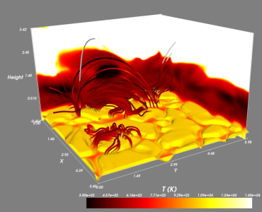
Figure 6.2: Three-dimensional visualization of the data cube temperature. The tubes represent the magnetic field lines (background tubes) and the velocity (foreground tubes).

In Fig. 6.3, we draw some portions of the isosurfaces of optical depth unity for the IR triplet lines. These corrugated surfaces are being modified at each point by the vertical velocity field (whose modulus is indicated with the color of the surface). We see that there is not a fixed height associated with the chromosphere, but a vertical range in which the plasma has the values of density, temperature and magnetic field that we identify as chromospheric layers. This region is constantly bubbling up and down as a consequence of the upward motions originated from the photosphere and amplified by the density gradient along the chromosphere. The increment of the vertical velocity is thus a result of the conservation of energy in the fluid. So, the macroscopic motion pass to be temperature-activated in the photosphere and below (granular convection) to density-enhanced from the chromosphere upward, leading to an expansion and a radiative cooling. The process is continued by gravity during the chomospheric downflows, in which the potential energy is transformed into kinetic and internal energy, arising temperature again. The model is a snapshot of that process.

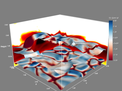
Figure 6.3: Three-dimensional visualization of the vertical velocity in the data cube. The background planes represent the temperature variation and give a reference about where the chromosphere ends. The component $\mathrm{V_{z}}$ is represented by the color of the surfaces, showing between $-3\,\mathrm{km\,s^{-1}}$ and $3\,\mathrm{km\,s^{-1}}$. The corrugated horizontal surface with L-shape nearest to the reader is defined by the heights of $\bar{\tau}=1$ for the $8498$ Å line. The other two corrugated surfaces are the same for $8542$ Å (towards the right) and the K line (the big “bubble” shape to the left).

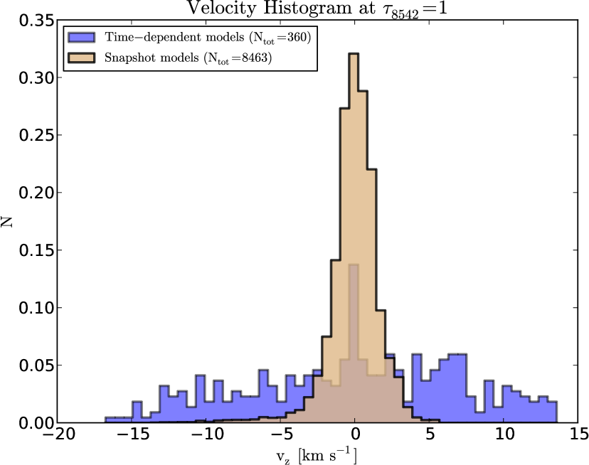
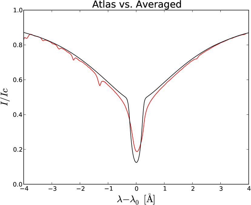
Figure 6.4: Left: vertical velocity distributions (normalized to unit area) of the 3D model analyzed in this chapter (orange) and of the strongly-dynamic 1D dataset analyzed in Chapter 5 (violet). The velocities are taken at $\tau=1$ for the $8542$ Å line. Right: Synthetic average intensity using a microturbulent velocity of $\mathrm{3.5\,km\cdot s^{-1}}$ (black line) and average intensity extracted from the Kitt Peak Solar Atlas (red line). Case of the $8542$ Å line at disk center.

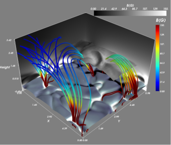
Figure 6.5: Visualization of the magnetic field topology of the data cube. The colors in the granules surface have no colorbar, it just represent the component $\mathrm{B_{z}}$, saturated between $-500$ G (black) and $500$ G (white) to identify the photospheric flux concentrations. The rest of surfaces and lines are coloured with the magnetic field intensity, saturated to $150$ G. The tubes represent some magnetic field lines. The corrugated horizontal surface is defined by the heights of $\tau=1$ for the $8542$ Å line.

The maximum velocity in the photosphere is around $4.3\,\mathrm{km\,s^{-1}}$. The velocity stratification patterns are similar to the ones in the time-dependent models of Chapter 5, but they differ notably in the maximum values and their statistical ocurrence. They do not have to coincide because one model is a temporal evolution and the other is a spatial mapping. Furthermore, we also have to realize that the LOS chosen in these new calculations is $\mu=1.0$, while the calculations in previous chapters were for $\mu=0.1$. Because of it, the emergent spectral lines will be now more sensitive to lower layers than they would be for a limb observation. Among other things, this means that the vertical velocities in the formation region of the spectral lines will tend to be smaller and the magnetic fields will tend to be stronger. Normalized histograms of chromospheric velocity allow a comparison between both set of models (fig. 6.4). The maximum velocity in the upper chromosphere reaches $12\,\mathrm{km\,s^{-1}}$, but such large values are scarce in its spatial distribution, being a value of around $5\,\mathrm{km\,s^{-1}}$ more representative. With these velocities we would not expect significant linear polarization amplifications induced by dynamics. However, we also have to take into account that the velocity component along the line of sight will be larger now because we look at disk center, directly in the direction of the motion.

Computing the emergent intensity and comparing with observations, the authors of the atmospheric model (Leenaarts et al., 2009a) extract some relevant conclusions that we reproduce here. The standard deviation of the central wavelength of the $8542$ Å intensity profiles with respect to the central wavelength of the average intensity is $\sim 50\%$ less than in real solar observations. On one hand, this means that there is a lack of macroscopic dynamics in the model, something to remember when analyzing the polarization profiles. But they also point out that the main reason of the difference is that the individual profiles are already narrower than in the Sun, implying that the real chromosphere is also more dynamic on scales not resolved by the simulation. Hence, the added microturbulent velocity is again justified in our calculations.

Concerning the magnetic field, Fig.6.5 illustrate a detail of the general topology of the magnetic field lines and intensities. Photospheric intergranular regions with high concentrations of magnetic flux and different polarities are the source of magnetic loops crossing the cromosphere. The magnetic intensities have typical values of a quiet Sun region.

A good way of grouping much of this information is drawing the main physical quantities (Fig. 6.7 and Figs. A.1, A.2 in Appendix A.4) at the approximated formation heights for each line. The heights at optical depth unity are shown in Fig. 6.6.

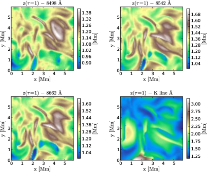
Figure 6.6: Heights of $\tau=1$ for the spectral lines under consideration. We can use the K line picture to identify expanded or compressed atmospheres because there is a correlation between this feature and the heights where the K line optical depth is unity.

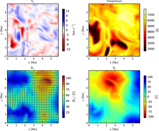
Figure 6.7: Physical quantities at $\tau=1$ for the $8542\,$ Å line. Upper left: vertical velocity. Upper right: temperature distribution. Note the cool patches. Lower left: horizontal magnetic field intensity. Lower right: longitudinal magnetic field intensity.

In the next section, we will need to clasify each model into three simple thermodynamic categories: static FALC-like models, which are an intermediate reference, having a hot chromosphere from the minimum of temperature to the TR, but without extra heatings like shocks and compressions and without extra cool or extended plateaus of minimum temperature; hot models, typically more compressed and hotter than FALC; and cool models, typically more expanded and cooler than the others. They are very poor representations of the large variability found in the dataset but have to be understood as extreme cases where some of the features we describe in the following sections happen very frecuently. Each of these categories can have a chromosphere significantly moving upward, significantly moving downward or without a significant movement.

6.2 Synthetic polarization profiles in forward scattering.

In forward scattering geometry at disk center, the Hanle effect can create polarization in presence of inclined magnetic fields (Section 2.4). The symmetry breaking produced by such magnetic fields then gives us access to the thermodynamic and magnetic state of the plasma through the Hanle-induced Stokes Q and U signals and the effect that the anisotropic illumination has in the atomic system. In the following, we analyze the results of synthetizing the Stokes profiles in the 3D atmospheric models under such circumstances.

6.2.1 Individual profiles.

From each pixel/column of the model we obtained a Stokes vector (I,Q,U,V) as a function of wavelength for each spectral line of the atomic model. The variety of these spectral profiles is wide. A first classification of the emergent Stokes profiles can be done according to the inclinations of the magnetic fields producing them. The set of Stokes vectors with significant linear polarization is caused mainly by a predominantly horizontal magnetic field (say, with $\mathrm{|\cos{\theta_{B}}|<1/\sqrt{3}}$). They define what we will call Horizontal Field (HF) regions, which have magnetic field lines with the Van-Vleck inclination at their frontiers and are located between areas whose magnetic vectors are mainly vertical. Some examples of the profiles in the HF regions are shown in Fig. 6.8. Here, in areas with enough magnetic field inclination in the chromosphere, the pixels showing higher Doppler shifts have also larger amplitudes and qualitatively reproduce some features of the Doppler-induced modulations analyzed in previous chapters. The complementary regions will be called Vertical Field (VF) regions because the chromospheric magnetic field is there predominantly vertical. They are characterized by Stokes vectors with small Q and U but large V.

In general, the profile shapes in the HF regions resemble the ones analyzed in previous chapters (see Fig. 4.8). However, the shape of the linear polarization profile that was frequently associated with the $8498$ Å line appears now interchanged with the shapes of the $8542$ Å and $8662$ Å profiles in many pixels of the snapshot models. Namely, the $\lambda 8498$ Q$/$I signal resulting from FALC had always a valley at line center and the $8542$ Å and $8662$ Å had always a single peak. Now, the shapes are often interchanged, with the $8542$ and $8662$ Å lines presenting a valley and the $8498$ line presenting a peak (black curves in Fig. 6.8).

Such changes are not intrinsically produced by the velocity because they are also present when the calculation is repeated in static regime. As we explain next, the variations appear when passing from limb observation to disk-center observation, but are not always visible because the Doppler shifts and the thermodynamic effects on the anisotropy also play a role.

With Fig. 4.10 and Eq. (4.13), we can understand such intrinsic shape changes related with the LOS. In that figure, the vertical variations of the upper and lower level fractional alignments are fixed by the anisotropy of the radiation field, which is intrinsic to the model and does not depend on the LOS. Then:

1) When the inclination of the LOS varies, the main height of formation also does, so it can be above or below the cross point where the curves of the upper and lower level fractional alignments intersect (hereafter, the alignments intersection).

2) The key point is that the emerging fractional polarization at each wavelength is the result of a competition between upper and lower level alignments, whose net contributions at different layers can be positive or negative. A simplification of such competition is given by Eq. 4.13, which only considers the layer at $\tau=1$. Thus, at layers below the alignments intersection, the net contribution of both levels alignment to the emergent polarization has a certain sign. But above the cross point, such contribution has opposite sign.

3) If most of the layers contributing to the emergent spectral polarization in the formation region are well above (or well below) the cross point, their contributions to the fractional polarization will have the same sign everywhere. The net result will be a profile shape monotonic from the continuum to the line center. Hence, a single peak profile.

4) However, if the height of formation is near the alignments intersection, the contributing layers situated just above this point and the ones immediatly below will have opposite signs (they somewhat cancel out). Since they form the spectral line core, the result is a depression in the emergent linear fractional polarization at line center, hence, a valley.

In conclusion, the shape (two peaks versus one peak) of these spectral lines is modified by the relative position of the main region of formation with respect to the height of the alignments intersection. This fact could be used to evaluate the realism of the model atmospheres or to compare among them in certain observational configurations of reference, with the caution that the velocity gradients (or any other modifier to the anisotropy) are able to add their own effects.

In addition to the linear polarization, we can study the Stokes V profiles generated by the Zeeman effect of the longitudinal field component (Fig. 6.9). Their variability is also rich. It is frequent to find V profiles with two antisymmetric lobes whose signs depend on the sign of the longitudinal magnetic field component. The asymmetries they show are due to the coexistence of vertical velocity and magnetic field gradients, as is well-known from previous works (Sánchez Almeida et al., 1989; Landi Degl’Innocenti & Landolfi, 2004). More complicated patterns arise in the shape of Stokes V (red profiles in Fig. 6.9) in the presence of velocity gradients (intensity shape very assymetric) or heatings in the plasma (intensity in emission).

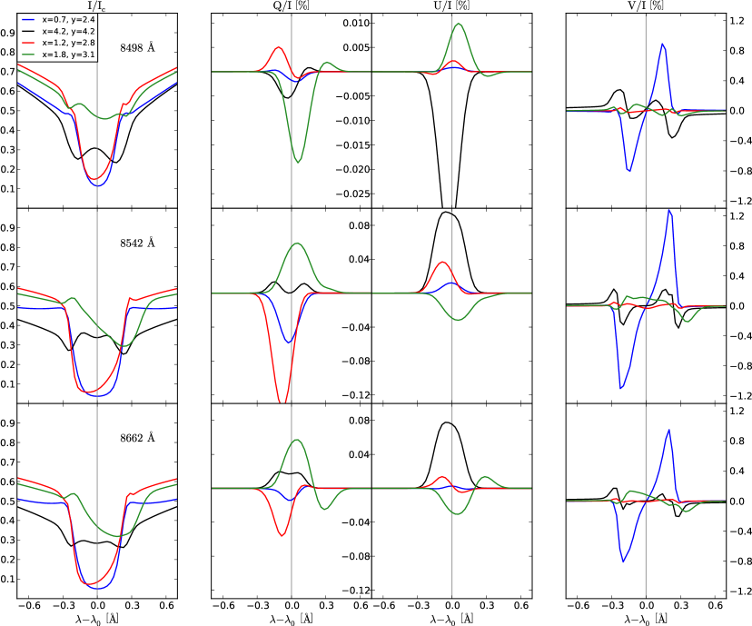
Figure 6.8: Examples of typical Stokes profiles of the IR triplet lines at four random pixels (different color means different pixel) where the magnetic field is predominantly horizontal at the chromosphere.

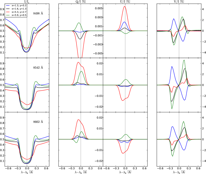
Figure 6.9: Examples of typical Stokes profiles of the IR triplet lines at four random pixels (different color means different pixel) where the magnetic field is predominantly vertical.

6.2.2 Slit profiles.

Simulating the profiles along a spectrograph’s slit, we can take a quick look to many spectral profiles at the same time. In Fig. 6.10, we show the synthetic map of the Ca ii $\lambda 8542$ intensity at line center, with coloured lines representing two slits. The corresponding slit profiles in the adjacent panels are identified with the coloured line at central wavelength. We have analyzed their main features using the Solar Inspector tool (see Sec. 3.4).

The intensity spectra of Fig. 6.10 show regions with emission in the wings and in the core, not always coinciding both features in the same profile. These intensity increments have different origins. The extra emission in the wings are due to heating by photospheric compression (sometimes associated with a photospheric bright point). In such a case, the downward plasma is compressing the photospheric layers while most of the low chromosphere and the temperature minimum region are almost at rest. When a pixel is associated with a bright point there is an additional increment of the magnetic field strength in lower atmospheric regions that produce large Stokes V signals. That is the case at $\mathrm{y\sim 2\hbox{${}^{\prime\prime}$}}$ and $\mathrm{y\sim 6\hbox{${}^{\prime\prime}$}}$ in the blue slit.

The extra emission in the line core (e.g., at $\mathrm{y\sim 4.5\hbox{${}^{\prime\prime}$}}$) is linked to Doppler shifts produced by motions in the chromosphere. In expanding atmospheres with motions located at the lower chromosphere, the blue shifts produced in the spectral radiation make those layers more transparent at line center wavelengths. Consequently, the excess of photons in upper layers produce medium and faint extra emissions in the intensity core. If medium/large velocities are compressing and shifting the chromosphere downward the effect is similar, but additionally the compression heats the plasma and can make the intensity to be completely in emission.

In pixels where the temperature gradient along the chromosphere is high enough, we also can appreciate reversal peaks at both sides of the line core intensities in the strongest IR lines ($\mathrm{y\sim 3\hbox{${}^{\prime\prime}$}}$). These features are similar to the K2 and H2 reversals appearing in the solar H and K lines (Linsky & Avrett, 1970) forming at top chromospheric layers in the Sun, but do not appear in solar observations of the $8542$ and $8662$ Å lines. Their presence in our results can indicate an unrealistic temperature stratification in the models (or a lack of temporal and spatial resolution in the observations). Other option is that they appear in our calculations because the microturbulent velocity is constant with height. Effectively, a variable microturbulent velocity at heights where the source function decouples from the Planck function can mixes the contributions from different layers and suppresses the reversals.

Some profiles with many of the mentioned features are shown in the blue slit panel of Fig. 6.10, at $\mathrm{y\sim 2\hbox{${}^{\prime\prime}$}}$. It corresponds to a region over a bright point. We see intensity emission in the core as well as in the wings. Accordingly, the atmospheric stratification shows a photospheric heating by compression (downward velocities below the temperature minimum) with upward velocities in the lower chromosphere that produce blue shifted radiation. A relatively intense vertical magnetic field at the upper photosphere is producing a notable Stokes V signal. Let us remind that the response function to the magnetic field in Stokes V is larger in lower layers for the $8542$ Å line. On the other hand, the abrupt change of sign in Stokes Q and U at $\mathrm{y\sim 2\hbox{${}^{\prime\prime}$}}$ has nothing to do with the previous reasons. It is indeed due to a weak magnetic field inclined almost horizontally in the chomosphere, whose azimuth changes from one pixel (showing $Q>0$ for example) to the next one (showing opposite sign). Thus, one Stokes vector can give clear information about the main physical magnitudes both at the chromosphere and the photosphere.

The largest linear polarization signals in such “slits” of Fig. 6.10 are mainly due to velocity gradients ocurring at places with a chromospheric magnetic field that is significantly horizontal. For instance, in the blue-slit panel, this happens at $\mathrm{y\sim 1\hbox{${}^{\prime\prime}$}}$ and $\mathrm{y\sim 4\hbox{${}^{\prime\prime}$}}$. The difference between the LP features at those points is that the latter corresponds to a compressive atmosphere and the former to an expansive one, which is less efficient increasing the anisotropy of the radiation field, but has in this case a strong velocity. In these pixels, the magnetic field strength is weak ($\mathrm{\sim 20G}$) at the chromosphere but also at the upper photosphere, which explains the absence of circular polarization.

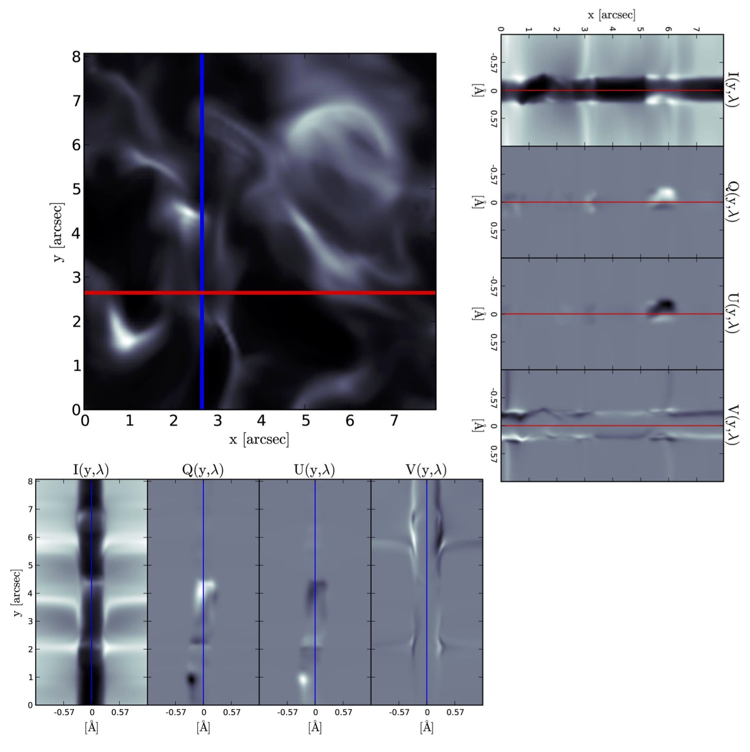
Figure 6.10: Emergent intensity map at $8542$ Å and two sets of synthetic slit-like Stokes profiles along the near-core wavelengths.

6.3 Maps of radiative quantities.

In this section we describe in more detail the spatial variations of the scattering polarization amplitudes taking into account different maps. Let us remind that in the forward scattering geometry we are considering in this chapter, the Stokes Q and U signals produced by an inclined deterministic magnetic field allow us to estimate the azimuth $\chi_{B}$ of the magnetic field. Setting the orientation of the LOS along the y axis ($\chi=-\pi/2$) in Eq. (2.50) we have:

$$\centering 2\,\chi_{B}=\,\arctan{\left(\frac{U}{Q}\right)}.\@add@centering$$ (6.2)

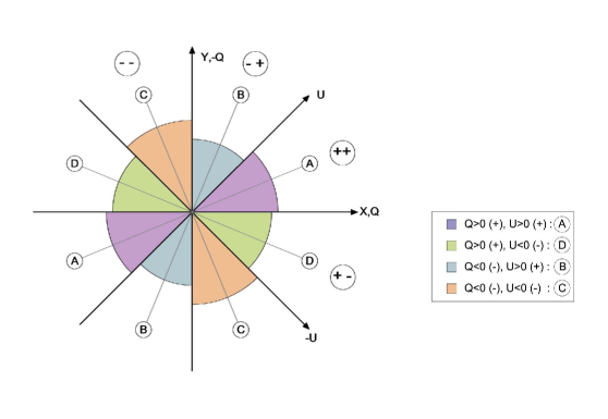
Figure 6.11: Observer reference frame for the linear polarization in forward scattering. The axes for Stokes Q and U specify the directions along which they are positive and negative in the reference system. The polarization plane is divided in coloured regions where the signs of the coordinates (Q,U) do not change. The directions A, B, C, D defined in those regions represent the $180\,\mbox{${}^{\circ}$}$ ambiguity.

The Hanle effect in forward scattering produces linear polarization along the projection of the magnetic field vector on the solar surface or along the perpendicular direction. In our calculations, we have chosen the positive reference for Q and U as indicated in Fig. 6.11, positive Q lying along the x axis (horizontal) and positive U inclined at $45$ degrees from the x axis. The directions of negative reference are perpendicular to the positive ones. As polarimetry is differential photometry, Stokes Q and U will be the difference between the number of photons oscillating in the corresponding positive axis and the number of them oscillating perpendicularly.

6.3.1 Maps of polarization amplitudes.

Figure 6.12 illustrates the maps of maximum Stokes Q and U separately for the $3934$ Å, $8542$ Å and $8498$ Å lines, following Eqs. (6.3). Line $8662$ Å is not shown here because it is very similar to $8542$ Å. For making these maps, the choice of other wavelengths (typically the line center) different from the ones corresponding to the maximum amplitudes results in notable signal losses in areas with substantial velocities.

$$\mathrm{\left(\frac{Q}{I}\right)_{max}} =\,100\cdot\mathrm{Max\left|\frac{Q}{I}\right|}\quad[\%]$$ (6.3a)

$$\mathrm{\left(\frac{U}{I}\right)_{max}} =\,100\cdot\mathrm{Max\left|\frac{U}{I}\right|}\quad[\%]$$ (6.3b)

In general, areas with significant linear polarization (LP) have always a magnetic field notably inclined (HF regions). Out of those areas, the LP amplitudes are always below $1/5$ of their maximum in the map.

In many pixels, the amplitudes have the same order of magnitude as those calculated by Manso Sainz & Trujillo Bueno (2010) in semiempirical models but, where we find velocities above $\mathrm{\sim 5\,km\cdot s^{-1}}$ in the chromosphere, we see relative enhancements that reach one order of magnitude in the amplitudes of the $8542$ Å and $8662$ Å lines. This is also true for the $8498$ Å line only if the model is not too cool. In sufficiently cool models, the $8498$ Å line always presents tiny linear polarization amplitudes (low-temperature patches in Fig. A.1 coincide with places of almost-zero polarization in both Q and U). The largest LP amplitudes in this line appear in Stokes Q and U in the absence of large velocities (Fig. 6.12, patches over $\mathrm{x\sim 4.5}$ Mm) and are twice larger than in the FALC model. Thus, the $8498$ Å anisotropy is affected by the velocity but seems to be dominated by temperature in the current models.

The differences between the Q and U maps are understood with Fig. 6.11. When the magnetic field existing in a region experiences a change in its azimuth, the polarization patches stand out in Q and attenuate in U or viceversa, so giving us an idea of the likely approximate directions of the magnetic field just by comparing regions. Patches with large Stokes Q and low Stokes U indicate that the field is chiefly oriented along some of the reference axes for Q (vertically or horizontally in the maps). If the opposite holds, the field is then mainly oriented in directions lying at $\pm 45$ degrees. If Stokes Q and U have similar amplitudes, it means that the field is in between the previous four directions.

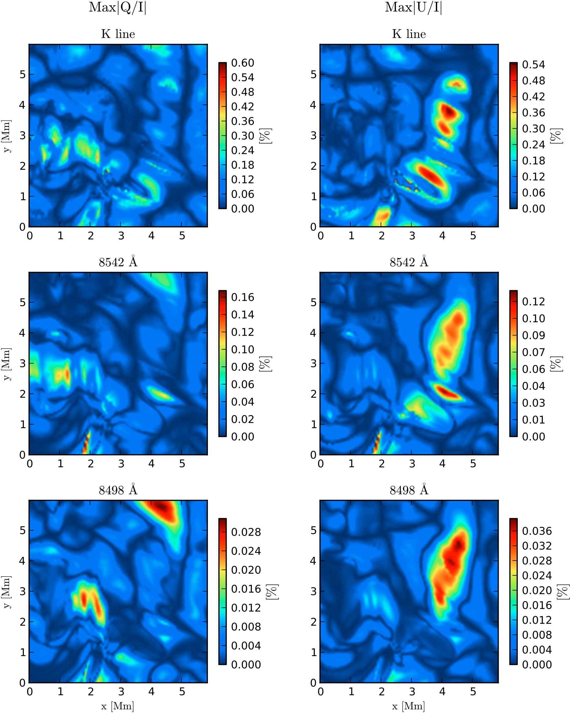
Figure 6.12: Maximum fractional linear polarization amplitudes across the solar model at $8498$ Å (lower row), $8542$ Å (middle row) and $3934$ Å (K line, in the upper row).

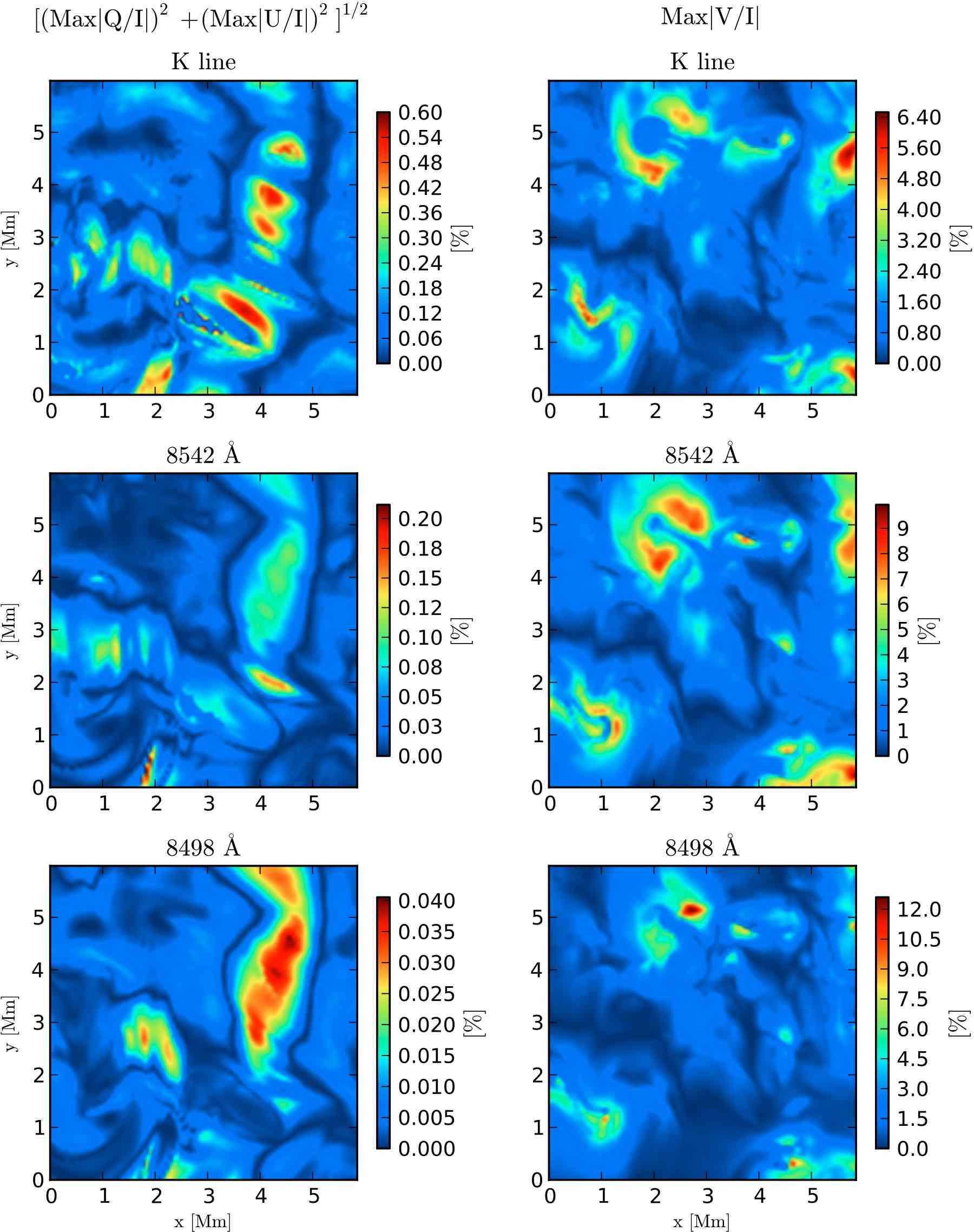
Figure 6.13: Calculated polarization amplitudes across the solar surface at $8498$ Å (lower row), $8542$ Å (middle row) and $3934$ Å (K line, in the upper row). Left: total linear polarization amplitudes calculated as $\mathrm{\sqrt{Max|Q/I|^{2}+Max|U/I|^{2}}}$. Right: The maximum of the absolute value of the fractional circular polarization.

The total linear and circular polarization are shown in Fig. 6.13. In that figure we see the spatial distribution of the maximum values (that is, at the wavelength of the maximum in each pixel) of the total fractional linear polarization (left panels) and fractional circular polarization (right panels) for the same three spectral lines. The places of negligible circular polarization are the ones where the magnetic field is almost horizontal at the heights of formation of the corresponding spectral line. The same region has larger linear polarization in the left panels (HF region). The strongest linear polarization patches in the $8498$ Å line are where the temperature is larger. However, the strongest linear polarization patches in the $8542$ Å line are where the vertical velocity is larger. The circular polarization in the $8542$ Å line is specially sensitive and clear marking the vertical magnetic field concentrations. Its value at each pixel is roughly twice the corresponding ones in the K line.

6.3.2 The Hanle Polarity Inversion Lines.

In the maps of Stokes Q and U (Fig. 6.12) we observe something interesting: the lines of zero linear polarization in Hanle forward scattering. They are groove-like regions whose emergent Stokes Q and/or Stokes U are virtually zero. They encode the topology of the magnetic field pervading the solar model.

We identify three kinds of Hanle Polarity Inversion Lines (Hanle PILs) produced by three different sources that can act together. Eqs. (2.48) evaluated in the frame of reference of Fig. 6.11 (and using $\chi=-\pi/2$ for the LOS) give a mathematical support for the following analysis in forward scattering:

$$\frac{Q}{I} \simeq\,-\frac{3}{4\sqrt{2}}\cos{2\chi_{B}}\cdot\sin^{2}{(\theta_{B})}\cdot(3\cos^{2}{\theta_{B}}-1)\cdot\mathcal{F},$$ (6.4a)

$$\frac{U}{I} \simeq\,-\frac{3}{4\sqrt{2}}\sin{2\chi_{B}}\cdot\sin^{2}{(\theta_{B})}\cdot(3\cos^{2}{\theta_{B}}-1)\cdot\mathcal{F},$$ (6.4b)

with all the r.h.s. quantities evaluated at $\tau=1$. Remind that these expressions are valid for a line in the saturation regime of the Hanle effect, which holds for the $\lambda 8662$ line in our dataset and very likely in real quiet Sun regions. If the field is weak but still strong enough, the other scattering signals of the triplet can also be saturated (especially $\lambda 8542$). Then, their geometrical dependence will also be described by Eqs. (6.4b).

The first kind of Hanle PILs are due to the inclination of the magnetic field. They are the same in Stokes Q and U (hence also in the total linear polarization) because they are independent of the magnetic field azimuth. They can be found delimitating regions in which the magnetic field is mainly horizontal (i.e., bordering areas with null longitudinal Zeeman polarization in Stokes V) or placed where the magnetic field is mostly vertical. Namely, they are always where $\theta_{B}=90\pm 35.27\,\mbox{${}^{\circ}$},90\pm 90\,\mbox{${}^{\circ}$}$, as confirmed by Eqs. (6.4). When at $\theta_{B}=90\pm 35.27\,\mbox{${}^{\circ}$}$ (magnetic field forming Van Vleck angles with the vertical), they are the frontiers between HF and VF regions. For this reason, we call them Van Vleck HPILs. They connect pixels with the same inclination. As the magnetic field emerges in bipolar structures at all scales, the Van Vleck HPILs have to form a closed line surrounding one of the magnetic poles.

The second kind will be called azimuthal HPIL. Namely, a Hanle PIL appearing in a map of Stokes Q (or Stokes U) is of azimuthal type if it does not appear in the same place for Stokes Q than for Stokes U. Clearly, they depend on the azimuth of the magnetic field in the chosen reference system (terms in $\chi_{B}$ in Eqs. (6.4)). In pixels defining an azimuthal HPIL in Stokes Q, the magnetic field vector is lying along the positive or negative reference directions for Stokes U. And viceversa, the pixels defining it in Stokes U have a magnetic field vector lying along the positive or negative reference directions for Stokes Q (see Fig. 6.11). Note that following an azimuthal HPIL, we connect pixels with the same magnetic field azimuth. Note also that, when two or more of them intersect, the cross point must have a magnetic field completely vertical. Consequently, they have a radial nature, beginning in an area of concentration of photospheric magnetic flux and ending in another one.

Finally, a third possible origin of a HPIL is a particular configuration of the anisotropy of the radiation field persisting across a region in the maps. They are thermodynamically induced HPILs and appear at the same time in the Q and U maps for a spectral line, as the Van-Vleck type ones. To grasp some feeling about the conditions in which they form, note that the thermodynamical HPILs gives zero linear polarization because the non-magnetic factor $\mathcal{F}$ in Eqs. (6.4) is negligible. Thus, we can pose the expression

$$\mathcal{F}=\omega^{(2)}_{J_{u}J_{\ell}}\sigma^{2}_{0}(J_{u})-\omega^{(2)}_{J_{\ell}J_{u}}\sigma^{2}_{0}(J_{\ell})=0.$$ (6.5)

In the simplest case, given by the line $8662$ Å, it yields the condition

$$\centering\sigma^{2}_{0}(J_{2})=\frac{\rho^{2}_{0}(J_{2})}{\rho^{0}_{0}(J_{2})}=0\quad{\rm at}\quad\tau^{8662}=1\@add@centering$$ (6.6)

How can such a condition be fulfilled?Let us suppose we have identified a thermodynamic HPIL, which appears at the same time in Q and U maps for the $8662$ Å line. Thus, consider the case in which Eq. (6.6) is satisfied in that region. It happens when the alignment $\rho^{2}_{0}(J_{2})$ tends to zero, or when the overall population $(\varpropto\rho^{0}_{0}(J_{2}))$ increases or when both things happen at the same time. A larger level-2 population can be achieved with an increment of temperature in the upper parts of the chromosphere. Such increment strengthens the Ca ii H line intensity emission (forming at the top), which illuminates lower chromospheric layers from above. The extra illumination arriving at chromospheric layers immediately below (where the $8662$ Å line originates) increases the population pumping from level 1 to level 4 which, in turn, produces an extra population in level 2 by spontaneous emission (see Fig. 4.1). Higher temperature thus means more population in higher energy levels (levels 4 and 5) and more emission (at $8662$ Å) produced by electrons falling from level 4 to level 2. Furthermore, if at the same time the formation region of the $8662$ Å line is meaningfully cool, the absorption of electrons from level 2 to level 4 will vanish, so retaining the population in level 2 (absorption to level 5 can be also neglected). If the absorption is very reduced from level 2 to level 4, the $8662$ Å line cannot be polarized because its polarization can only be generated by dichroism (selective absorption).

On the other hand, to have an almost null alignment in level 2 we need a formation region illuminated with a radiation field that cancels out the component $\bar{J}^{2}_{0}$. Outside LTE, it can occur in very especific situations, when the contribution of the mainly horizontal illumination equals the contribution of the vertical one in the evaluation of the anisotropy at those layers. We can show that it happens in pixels that separate areas where the formation region is significatively cool from areas having a formation region at relatively large temperatures. If, furthermore, the HPIL is in a place without significant velocity gradients, the low existing alignment will not be enhanced by dynamics.

The previous explanation for Eq. (6.6) seems to be correct in the borders of a cool chromospheric plasma bubble appearing in the solar models. There, the polarization in Q and U is zero. To examinate this observation, we first identified the location of the thermodynamical HPIL in the Stokes maps. Then, with 3D visualizations (see stereographic view in Appendix A.5), we verified that the cool bubble has a singular stratification at its enclosing verticals. In the interior of the bubble, the chromospheric temperature is as cool as $3000$ K and the anisotropy is dominated by vertical radiation coming from above the bubble and also from the photosphere. On the contrary, the plasma at the external surroundings of the bubble is much hotter in the formation region of the spectral line. Consequently, the horizontal radiation dominates, changing the sign of the alignment with respect to the interior of the bubble. In the middle of both regions (the bubble’s frontier), a line where the net alignment is zero must exist because it is positive at one side and negative at the other. That is a thermodynamical Hanle PIL and it has been induced by spatial differences of temperature.

An example of cool bubble is found around $\mathrm{(x,y)}=(3.8,1.5)$ Mm in the upper-right panel of Fig. 6.7. The corresponding HPILs appear in Stokes Q and U maps of the $8662,8542$ and $8498$ Å lines, surrounding the region. For example, a part of the null line is connecting the points $(3.5,2)$ and $(4.5,1)$ Mm. We conclude that a way of distinguishing a thermodynamic HPIL from a Van-Vleck HPIL is searching the former around cool patches.

The HPILs could give us extra information. For example, the contrast and width of a Hanle PIL gives information about the variation with height of the magnetic field along the formation region of the considered spectral line. The differences in width between HPILs pertaining to spectral lines forming at different heights complement that information. Besides that, a histogram of the mean size of the regions enclosed by the HPILs could be a quick way of measuring the variability of some magnetic field parameter (helicity, inclination, azimuth) in a map. It could be used as a fine tester to a model atmosphere in order to compare the polarization fingerprints it produces with the ones in high-sensitivity solar observations. In Section 6.6, we will explain some criteria based on HPILs in order to infer the magnetic field topology.

In principle, we see two objections to the observational potential of the HPILs. First, the practical application of these ideas is very difficult given the current polarimetric sensitivity. And second, diffuse light due to internal reflections in the optical system preceding the detector can play a role in masking the HPILs because it diminishes the contrast between regions with and without polarization.

We conclude that the Hanle PILs in the Ca ii IR triplet are true fingerprints encoding the orientation of the chromospheric magnetic field. Perhaps more than that, the HPILs could offer new diagnostic aids to capture very specific circumstances of the thermodynamical state in the atmosphere. Overcoming the technical impediments, we see possible to deduce the three-dimensional topology of the chromospheric magnetic field from 2D maps of the Stokes vector (Sec. 6.6.2). Some extra calculations (Sec. 6.5.2) suggest that these structures with null polarization could likely be distinguished for the first time with the coming instrumental solar facilities (Zimpol 3, EST, Solar-C). The HPIL concept leads to an interesting question: can we get a precise magnetic field mapping using the spatial locations where the polarization amplitudes cancel?

6.3.3 Maps of the Polarization Degree.

The degree of linear and circular polarization of the Stokes signals measure the total amount of linearly and circularly polarized light for a whole spectral line. They are calculated by integrating the contributions of photons in a certain spectral window in order to increase the signal to noise ratio. The expressions we have used to calculate them are

$$\mathrm{LPD}\,[\%] =\,100\cdot\frac{\sqrt{\left[\overset{\lambda_{2}}{\underset{\lambda_{1}}{\sum}}Q\right]^{2}+\left[\overset{\lambda_{2}}{\underset{\lambda_{1}}{\sum}}U\right]^{2}}}{\overset{\lambda_{2}}{\underset{\lambda_{1}}{\sum}}I},$$ (6.7a)

$$\mathrm{CPD}\,\left[\%\right] =\,100\cdot\frac{\overset{\lambda_{2}}{\underset{\lambda_{1}}{\sum}}|V|}{\overset{\lambda_{2}}{\underset{\lambda_{1}}{\sum}}I},$$ (6.7b)

where the wavelengths $\lambda_{1}$ and $\lambda_{2}$ delimit the width of the filter considered in the integration.

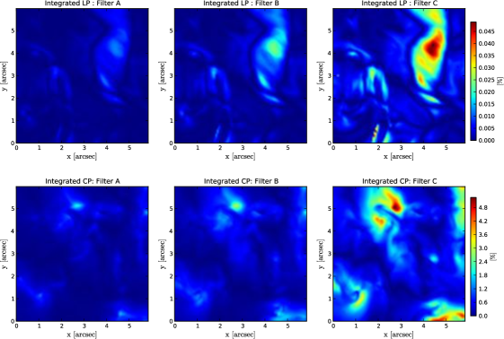
Figure 6.14: Spatial maps of linear polarization degree (top panels) and circular polarization degree (bottom panels) calculated (Eqs. 6.7) by integrating around $8542$ Å with three different filters. Filter A(left column): filter with a width $\mathrm{\Delta\lambda\sim 2}$ Å. Filter B(middle panels): $\mathrm{\Delta\lambda=1.2}$ Å. Filter C(right panels): $\mathrm{\Delta\lambda=0.7}$ Å. Each colorbar is common for a row of panels.

We have obtained these quantities for our dataset in three different square filters placed at line center: the filter A ($\Delta\lambda=2$ Å), which reaches wavelengths in the far wings of the line; the filter B ($\Delta\lambda=1.2$ Å), which selects the core and near wing of the line; and the filter C ($\Delta\lambda=0.7$ Å), which only captures the core of the line, where the linear polarization is more significant. The results for the $8542$ Å line are shown in Fig. 6.14. In Fig A.3 we show similar results for the K line.

The filter C is the most suitable because it allows a clearer contrast between regions with and without polarization. Filters A and B produce lower fractional polarization signals because the wings intensity contribution in the denominator of Eqs. (6.7) is much larger than the integrated polarization at those wavelengths. We have to reach a trade off between signal gains by integration and signal losses by the excesive number of non-polarized photons at the wings. Note also that in general the resulting numbers for the polarization are not representative of the real maximum polarization amplitude. This is because the Eqs. (6.7) are not linear in the Stokes parameters. Thus, the advantage of calculating the polarization degree maps is mainly to get a better signal to noise ratio, so showing structures with more contrast and definition than the fractional polarization at one wavelength.

6.3.4 Maps of polarization contrasts.

In this section we show that the identification of drivers and situations changing the linear polarization signs may allow us to infer extra information about the solar atmosphere. It also helps us to deduce correctly the direction of the magnetic field, for what it is previously necessary a discrimination of all the drivers affecting the polarization sign (polarity) at each pixel. To that end, the maps of polarization contrasts (Fig. 6.15) are useful to determine the main regions where the different drivers have to be disentangled as well as the polarization sign in those regions. We remind that the polarization contrast is basically a peak-to-peak amplitude with an artificial sign indicating whether the largest peak is positive or negative.

The first thing we note in Fig. 6.15 is that the significative patches are highlighted in the HF region (to identify the HF region see lower left panel in Fig. A.8 for instance). This is because the polarization contrast, being a peak-to-peak measure, has more dynamic range than the absolute value of the polarization. Thus, for a similar color palette, the polarization contrast is more efficient (than the maximum polarization) highlighting the larger linear polarization signals, which are always in the HF region.

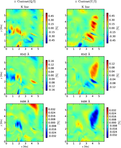
Figure 6.15: Signed contrast amplitudes for Stokes Q and U in the same spectral lines than in Fig. 6.13. Left: the signed contrast defined as the difference between the maximum and the minimum Stokes Q, where the artificial added sign is positive/negative if the maximum Stokes Q is positive/negative. Right: the same as in left panels but for Stokes U.

Reference signals in the saturation regime

To understand and “diagnose” the changes of sign in the polarization patches of Fig. 6.15, we will need to define a reference model atmosphere that: (a) is static, (b) has a hot FALC-type chromosphere, (c) has no extra heatings due to shocks or compressions, and (d) has a horizontal magnetic field in the saturation regime of the Hanle effect that lies parallel to the reference direction for $Q>0$ and to the x axis ($\chi_{B}=0,\theta_{B}=\pi/2$). The LOS is set along the y axis ($\chi=-\pi/2$). This configuration of reference gives the maximum LP amplitude for a horizontal magnetic field both in forward scattering and in a close-to-limb observation. The calculations done in such model will hereafter define a reference for the signs of the LP in the IR triplet lines.

Figure 6.16: In the reference configuration $\chi_{B}=0,\,\theta_{B}=\pi/2,\,\chi=-\pi/2$ and $Q>0$ is parallel to x. The line of sight (LOS) can be $\mu=0.1$ or $\mu=1.0$. The vertical axis is the solar radial direction passing through the point considered.

From Eqs. (2.47), it follows that both the $\mu=0$ and $\mu=1$ polarization amplitudes resulting from such a reference configuration are a half of the maximum possible amplitude (given by the non-magnetic case in a limb observation):

$$\bigg{(}\frac{Q}{I}\bigg{)}^{\rm ref} \Rightarrow\bigg{(}\frac{Q}{I}\bigg{)}^{\mu=0}_{\theta_{B}=\pi/2}=\bigg{(}\frac{Q}{I}\bigg{)}^{\mu=1}_{\theta_{B}=\pi/2},$$ (6.8a)

$$\bigg{(}\frac{Q}{I}\bigg{)}^{\rm ref} =\frac{1}{2}\bigg{(}\frac{Q}{I}\bigg{)}^{\mu=0}_{\theta_{B}=0}=\frac{1}{2}\bigg{(}\frac{Q}{I}\bigg{)}^{\mu=0}_{B=0}.$$ (6.8b)

In our forward-scattering case in which the polarization amplitude is roughly given by Eq. (6.4a), note that the reference sign of a Stokes Q signal resulting from the above configuration is the sign of the thermodynamical factor $\mathcal{F}$ of Eqs. (6.4). That is still true in any atmospheric model with $\chi_{B}=0\,\mbox{${}^{\circ}$}$ and with a $\theta_{B}$ corresponding to the HF region.

Polarization signs as physical references

Now, we explain Fig. 6.15 and some differences of sign found between the spectral lines analyzed. First, the linear polarization (LP) patches in the maps of $\lambda 8542$ (and $\lambda 8662$) have opposite sign to the corresponding ones for $\lambda 8498$, which is a typical behavior in the IR triplet when the calculations are done for disk center. Such signs difference holds in almost all pixels. It suggests that the difference of signs between the $8542$ and $8498$ Å lines is a essential and robust feature primarily set by the atomic coefficients contained in $\mathcal{F}$, but not significantly influenced by anisotropy variations.

On the contrary, the difference of signs between the $8542$ Å line and the K line does vary between polarization patches. Sometimes, both lines share the same sign, sometimes not. In standard FALC-like models they should show the same sign, however. The reason of the change is not the magnetic field direction because it varies slowly between the medium-high ($8542$ Å line main formation region) and the top chromosphere (K line main formation region). We associate such change with strong spatial differences of temperature between both heights. It happens, for instance, in the cool chromospheric bubble around $(x,y)=[3.5,1.5]$ Mm (see Sec. 6.3.2), which was formed after the ascension of a shock. In that area, the LP maps show a patch with different signs in the $8542$ Å line and the K line. Thus, we identify the LP sign as a simple marker of strong chromospheric temperature gradients. Concretely, patches changing their sign between the $8542$ Å map and K line map indicate a large difference in temperature between the very top and lower parts of the chromosphere. This fact allows to estimate that the cool bubble reaches a height located between the medium-height and the top chromosphere.

With respect to the reference case, there are four basic drivers that alter the polarization sign of these IR triplet lines: the inclination of the LOS; some very specific circumstances for the temperature stratification (Sec. 6.3.2); the magnetic field; and the velocity gradients (Chapters 4 and 5).

Concerning the line of sight, when passing from the solar limb to the disk center, the signs of the $8542$ Å and $8662$ Å lines usually change because all the main contributing formation heights shift downward, below the level alignments intersection (recall Section 6.2.1 and Fig. 4.10) and it modifies the sign of $\mathcal{F}$. Thus, in our reference FALC-like model described previously, the Stokes Q sign for these lines would be $[+]$ at $\mu=0.1$ and $[-]$ at $\mu=1$. The $8498$ Å line already had low formation heights that do not change their net contribution to the polarization because they shift yet below the alignments intersection (towards even lower layers) when passing to forward scattering. Hence, this line does not change its polarization sign, which would be $[+]$ for both LOS in the reference FALC-like model.

Concerning the temperature stratification, the results of Manso Sainz & Trujillo Bueno (2010) in FALC models and forward scattering suggest that the IR triplet lines change their polarization signs between hot and cool models with the same magnetic field orientation. As already commented, that is also valid in our results. For example, the pixel at $[4,3]$ Mm and the one at $[4,1]$ Mm (see Stokes U in Fig. 6.15) have opposite linear polarization signs in the triplet lines because one pixel has a FALC-like chromosphere and other has an almost completely cool chromosphere. They have the same magnetic field orientation and negligible velocity. A similar situation occurs in the surrounding pixels, resulting in two patches with opposite polarization contrasts. Another example is the patch at $[2,3]$ Mm (hot) compared with the one at $[1,3]$ Mm (cool). Such behavior is less visible for the $8498$ Å line because its polarization tends to vanish in very cool chromospheres.

The reference model in a forward scattering geometry yields emergent Stokes-Q signals whose reference signs are $[+,-,-]$ for the $[8498,\,8542,\,8662]$ Å lines. Then, under similar circumstances but in cool-chromosphere models, the result is $[-,+,+]$. An example of such reference case is the blue patch at $[4.5,5.5]$ in Stokes Q $\lambda 8542$ (Fig. 6.15). Effectively, this patch is an almost static FALC-like region with an almost homogeneous chromospheric magnetic field that is parallel to the x axis (note the absence of Stokes U).

The explanation for the sign reversal is the dependence on the radiation field anisotropy on temperature. In a cool chromospheric model, the vertical radiation is more intense than the horizontal (positive net contribution to the anisotropy). In a hot model, with or without a temperature shock or heating in the formation region, the contrary holds: the net contribution to the anisotropy is negative. The $8498$ Å line is more sensitive to these changes because it forms lower (nearer the minimum of temperature and the alignments intersection), and when the plasma is cool there, its emission vanishes. The other lines of the model are mainly created nearer the transition region, for what they necessitate a cool stratification along the whole chromosphere (cool bubbles) to reverse their polarization signs.

Concerning the magnetic field, the azimuthal dependence in Eq. (6.4) allows us to deduce the expected polarization signs for other field azimuths without calculations, just following Figure 6.11. To do it, we must note that: for a hot FALC type model in the HF region, the signs of the emerging Stokes Q and U in the $\lambda 8542$ line for any magnetic field azimuth are always opposite to the signs of the corresponding Stokes Q and U axes that are nearest to the projection of the magnetic field vector in Figure 6.11.

For instance, if the reference FALC-like model had the magnetic field exactly along the +U axis, the signs for Stokes U would be $[+,-,-]$ with zero Stokes Q. If it were along -Q, Stokes Q would be $[-,+,+]$ with zero Stokes U. If such hot model would have the transverse component of the magnetic field in between the $+$Q and the $-$U axes, Stokes Q would be $[+,-,-]$ and Stokes U $[-,+,+]$. Besides this, the so-given LP signs can furthermore be modified by changes in temperature and velocity.

This is helpful. For example, consider the positive U patch around $[4.5,4]$ Mm in the LP contrast map of the $\lambda 8542$ line (Fig. 6.15) and suppose we only know it is a hot (FALC-like) model in the HF region (as it is). We then see that the patch has $U>0$ and $Q\sim 0$. Following the references, that configuration is only compatible with a magnetic field along the $-$U axis, which is correct. If the chromosphere model were cool, $\vec{B}$ should be along $+$U. In addition to that, we recall that the LP signs in the K line core and in $\lambda 8498$ can help to establish the presence of “cool bubbles” and large temperature gradients after a shock wave that has crossed the chromosphere. All together gives a “zero-order” diagnosis based on LP references.

Concerning the vertical velocity, we need to find out how it modifies the signs with respect to the static case. On one hand, we know that the velocity gradients can efficiently modulate the radiation field anisotropy (Chapter 5). In the case of the Ca ii IR lines, it directly enhances the lower level aligment at heights just above $\tau=1$ (see Fig. 4.10). On the other hand, we have evidences suggesting that the profiles with a valley at line center are prone to change their signs with a velocity gradient, while the single-peak ones do not (e.g., see Figure 4.8). These results suggest that a velocity gradient in the formation region of a spectral line can alter the balance between the upper and the lower level alignments that control the fractional scattering polarization. Thus, depending on the sign of the alignment at those layers (and on the intrinsic atomic polarizability coefficients, which have a certain sign), the line will have amplitudes enhanced or diminished with respect to the static results. The larger sentivity to this effect in valley-like profiles is because their formation regions are very near the alignments intersection. We have investigated this behavior in each model.

For example, in the calculations done in dynamic non-magnetic 1D models at $\mu=0.1$ (Chapter 5), the $8498$ Å line was the only one that changed its linear polarization sign in expanding or compressing atmospheres. We concluded that such changes in sign were possible due to a strong dynamics and to the proximity of the $\lambda 8498$ formation heights to the level alignments intersection, which furthermore made its LP profiles to vary their essential shape. In the current 3D models, the synthetic LP profiles of the $8498$ Å line in $\mu=1$ very rarely exhibit a valle-shape and we do not see clear indicatives of significant Doppler-induced amplifications in this line. This can be understood with the lower degree of dynamism (see Fig. 4.8) and a lower height of formation (see Sec. 6.2.1). On the other hand, the other two lines of the triplet can now exhibit a valley shape, and we wonder whether they can also reverse their polarization sign in presence of a velocity gradient as the $\lambda 8498$ line did at $\mu=0.1$. However, it seems that the proximity of the point of alignments intersection to the main heights of formation is not enough to produce a polarity reversal. In principle, the effect of a velocity gradient in these lines in the 3D models is only a modest variation of the amplitudes of Stokes Q and U with respect to the static case. It makes the resulting azimuth estimated from Eq. (6.2) to vary with respect to the real azimuth.

This last conclusion is relevant because it means that Eq. (6.2) can fail in the inference of the chromospheric magnetic field azimuth in situations where the vertical velocities are significant (dynamic fibrils, mottles and spicules).

General rules as the ones above and the specific situations breaking them are of interest for developing chromospheric diagnosis methods based on polarization. Thus, starting from a reference situation, we can try to simplify the variation of the LP signals referring them to some simple qualitative changes in the reference models. Thus, in models with a weak dynamic ($v\sim 0$), the basic behavior of the LP signals in the IR triplet can be summarized with Table 6.1.

$\mu=1$, $v\sim 0$ @ HF region
$\vec{B}$	Cooler	$\leftarrow$FALC-like$\rightarrow$	Hotter
$\boxminus$ (along $+$Q)	$[-,+,+]$	$[+,-,-]$	$[+,-,-]$
$\boxslash$ (along $+$U)	$[-,+,+]$	$[+,-,-]$	$[+,-,-]$
$\boxvert$ (along -Q)	$[+,-,-]$	$[-,+,+]$	$[-,+,+]$
$\boxbackslash$ (along -U)	$[+,-,-]$	$[-,+,+]$	$[-,+,+]$

Table 6.1: Signs of the LP in the Caii IR triplet in forward scattering and considering static models in the HF region ($54.73\,\mbox{${}^{\circ}$}<\theta_{B}(\tau=1)<125.27\,\mbox{${}^{\circ}$}$). The squared symbols represent the direction of the magnetic field in the plane of the sky. The signs in brackets correspond to each spectral line ordered as [$\lambda 8498$,$\lambda 8662$,$\lambda 8542$]. Such signs correspond to Stokes Q (when $\vec{B}$ is along $\pm$Q) or Stokes U (when $\vec{B}$ is along $\pm$U). Each column selects the stratification of temperature, which can have a cooler or hotter chromosphere than in FALC-like models. All the signs would be the opposite out of the HF region.

6.4 Effect of the vertical velocities.

We have computed the maps of polarization contrast, the maps of polarization amplitudes, histograms of total linear polarization and the spectral profiles again, but setting the velocity to zero in all points. With this information we analyze the influence of the dynamic on the linear polarization by paying attention to the amplitudes, to the sign of the maximum amplitude in each pixel and to the shape of the profiles.

Statistically, the effect of the velocity in the maximum amplitudes of the LP resulting from the 3D snapshot is small in comparison with the effect of the magnetic field and the temperature gradients. The maximum LP polarization value of the distribution of velocities (histograms in Fig. 6.17) changes from $0.13\%$ to $0.21\%$ when adding the velocity, which is a typical amplification in the light of the results from previous chapters. It indicates that the modulation produced by dynamics in the profiles has a certain influence. However, the histograms in Fig. 6.17 show that such effects are measurable in a low number of pixels, whose LP values “migrate” from lower to upper parts in the histogram (orange excesses in the distribution tails of Fig. 6.17). One reason for this relatively small number of LP signals with strong amplifications is that the velocity gradients in the formation region are not as large as in the time-dependent models. Indeed, the dynamic is comparatively much more reduced in the MHD models (Fig. 6.4). It has to be taken into account that we should expect stronger dynamic effects in the Sun (Leenaarts et al., 2009a). On the other hand, we have to consider that a small filling factor of enhanced signals does not necessarily mean a lack of significative effect along time.

In a non-negligible number of pixels, the “static” polarization amplitudes are already larger in the 3D dataset than in static semiempirical models. The results in FALC models (Manso Sainz & Trujillo Bueno, 2010) establish maximum LP amplitudes around $0.02\%$ in forward scattering, but we find pixels with LP values reaching $0.13\%$, an order of magnitude larger. In fact, most pixels in the HF region have amplitudes above the FALC values (Fig. 6.17, right panel). These amplitudes are a consequence of the larger chromospheric temperature gradients with respect to the FALC model. Since the linear polarization is a response to the anisotropy of the radiation field, a local variation of the limb darkening law produced by the temperature can effectively explain the new amplitudes seen in these static cases.

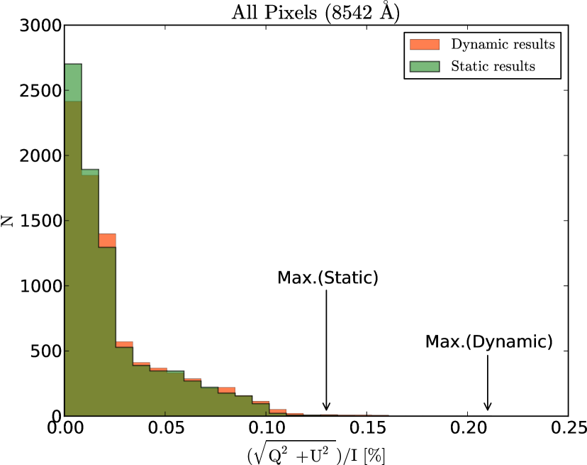
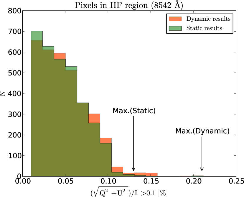
Figure 6.17: Histograms of the total linear polarization for the $8542$ Å line in the whole map (left panel) and only considering the HF region (right panel). The histograms are semi- transparent: a dark green color indicates that the orange distribution is behind the light green distribution.

Irrespective of the amplification factors, the effect of the velocity gradients in forward scattering are always a modulation of the LP signals with respect to the static case. As has been anticipated, the forward scattering geometry gives decreased amplitudes in many pixels due to the proximity of the formation region to the height where the upper and lower level fractional alignments become equal (Sec. 6.2.1). This makes the $8542$ and $8662$ Å lines alter their responses with respect to the $90$-degree scattering case, behaving similarly to the $8498$ Å line at limb observations. More explicitly, when the velocity gradient starts to increase, the LP signals become systematically more asymmetric with a decreasing amplitude and tending to become antisymmetric. If the velocity continues increasing, the signals are enhanced in amplitude but with a sign that is typically the opposite of that of the static case (reversal amplification: see Fig. 4.8, second right panel from the top). Therefore, if the velocity gradient is not very strong, the amplitude of the scattering signals can be smaller than in the static case. This behavior makes them more unpredictable because such signals are not limited to only one sign.

We already know (see Section 6.3.4) that a good tracer of such process is the polarization contrast (difference between the maximum and minimum value of the signals). The reason is that the contrast is always modified (generally enhanced) because the velocity gradients generate asymmetries whose total peak-to-peak excursions are usually larger than the static amplitudes. The artificial sign we add to the contrast corresponds to the maximum peak of the signal and help us to identify if a reversal amplification is being produced. Thus, comparing the static and dynamic maps of polarization contrasts we have seen that the signs of the maximum amplitudes at each pixel are never reversed. The only change is an increment of the contrasts that strengthens the patches in Fig. 6.15. That is why we conclude that the velocity gradients in the analyzed MHD models are not strong enough for putting the LP profiles in their amplification phase. This calculation confirm that the polarities of Stokes Q and U are not altered by the velocity (preliminar conclusion of Sec. 6.3.4). The stability of the polarities also allows to extend the validity of the reference signs in Table 6.1 to the dynamic case, which is correct for the present models but will not be true in situations with stronger dynamics.

A visual summary of the situation can be given following Fig. 6.18. The labels A, B, C, D, E and F identify the panels corresponding to some “static” pixels. The panel immediatly below each static case corresponds to the respective dynamic case for the same pixels. Only the F panels show the behavior of the LP in $\lambda 8498$, the other panel are for $\lambda 8542$ (the conclusions for this line are extended to the $8662$ Å line). The figure illustrates the following:

A

In some pixels, the $8542$ Å line behaves like in previous studies: it increases monotonically with the velocity (static and dynamic A panels). This would be the case of the pixels corresponding to the orange excesses in the histograms.

B

But a much more frequent behavior appears for these models: double-peaked profiles become asymmetric and decrease in amplitude in presence of velocity gradients (static and dynamic B panels).

$\begin{array}[]{ccc}\includegraphics[width=144.54pt]{8542_15x40ia.pdf}&\includegraphics[width=144.54pt]{8542_35x25ia.pdf}&\includegraphics[width=144.54pt]{8542_65x30ia.pdf}\\ \includegraphics[width=144.54pt]{8542_15x40ib.pdf}&\includegraphics[width=144.54pt]{8542_35x25ib.pdf}&\includegraphics[width=144.54pt]{8542_65x30ib.pdf}\\ \includegraphics[width=144.54pt]{8542_25x40ia.pdf}&\includegraphics[width=144.54pt]{8542_17x0ia.pdf}&\includegraphics[width=144.54pt]{8498_65x60ia.pdf}\\ \includegraphics[width=144.54pt]{8542_25x40ib.pdf}&\includegraphics[width=144.54pt]{8542_17x0ib.pdf}&\includegraphics[width=144.54pt]{8498_65x60ib.pdf}\end{array}$

Figure 6.18: Representative examples showing the effect of the velocity on the linear polarization in the considered MHD model. Grouped in pairs, the plots illustrate the $\rm{Q/I}$ signals in adjacent pixels when setting the velocity to zero (static case, labelled with a letter) and the corresponding results in the same pixels when velocity is activated (plot immediatly below the labelled one). Pairs A, B, C, D and E are for the $8542$ Å line and the pair F is an example for $8498$ Å. Stokes U presents similar patterns.

C

Both behaviors in panel pairs A and B are part of a same process that is clearly observed between adjacent pixels like being different timesteps of a similar temporal evolution (dynamic C panels).

D

The larger the amplitudes in absence of velocity, the larger the velocity gradient necessary to reverse the profile polarity. Thus, in our MHD models, the dynamic is usually insufficient to reverse the sign of the relatively large signals created by the temperature gradients. It results in the predominance of asymmetries and variable amplitudes (static and dynamic D panels).

C, D, E

In comparison with a limb observation, the larger velocity component along the LOS when looking at disk center can produce larger spectral shifts and broadened signals (dynamic panels in C, D and E).

E

Furthermore, the rich variability of the atmosphere produce extraordinary situations that can limit the amplification of the LP signals in the presence of significant velocity gradients. For instance, when there is a dense cloud or bubble with an homogeneous motion over a region with large gradient, its opacity softens the impact of the Doppler-induced anisotropy on the emergent polarization. So, in such accumulations of material (more usual above stronger magnetic fields) we see broader spectral signals but not necessarily large amplifications (static and dynamic E panels).

F

The $8498$ Å line follows a similar behavior. It also has larger amplitudes than in the FALC model due to the temperature, but it is poorly amplificated by the low- chromosphere velocities (static and dynamic F panels).

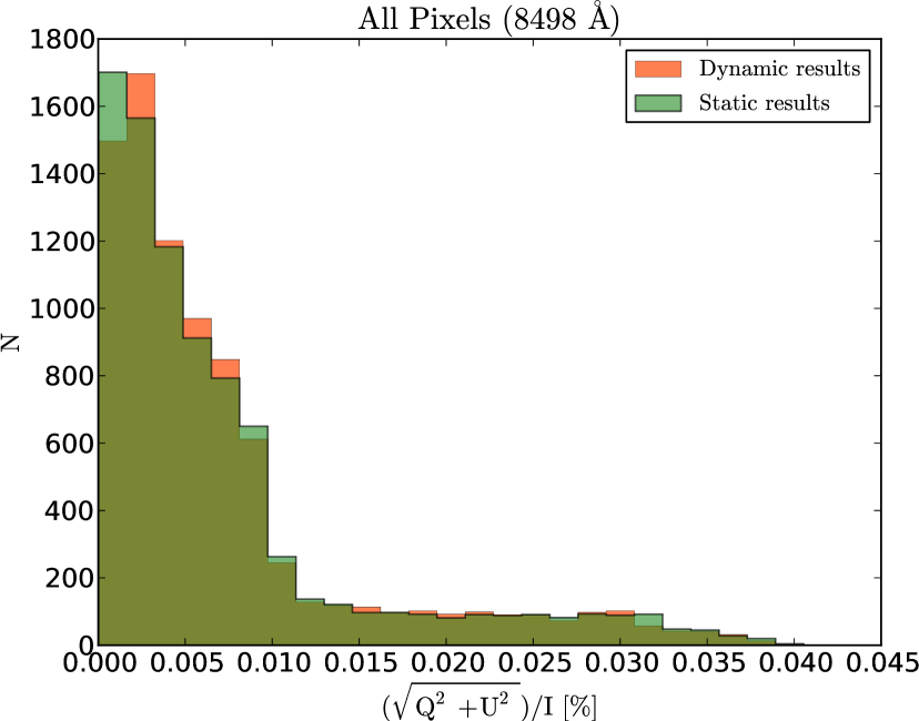
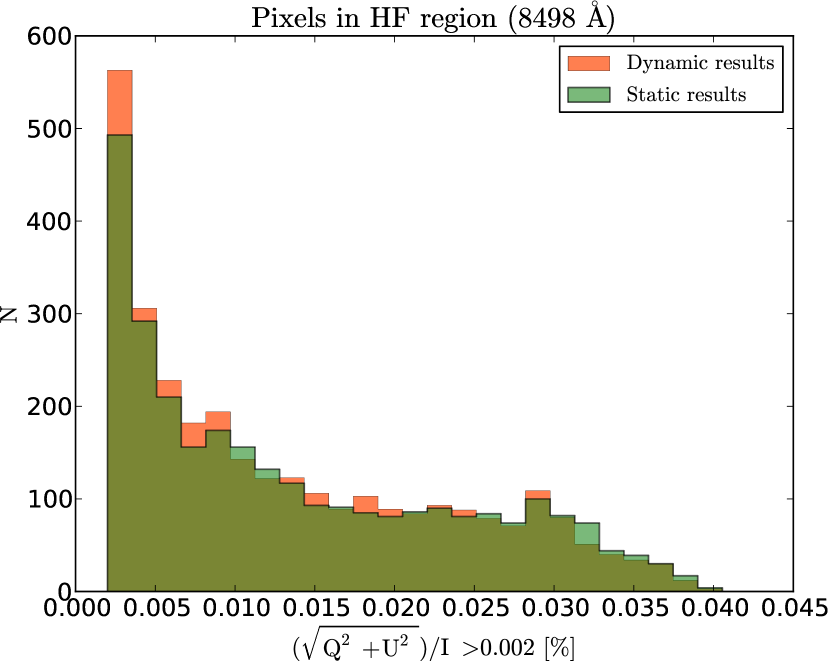
Figure 6.19: Histograms of the total linear polarization for the $8498$ Å line.

A remarkable difference in the $8498$ Å line with respect to the other spectral lines in the IR triplet is the longer distribution tail in the histograms of Fig. 6.19. The maximum amplitudes are produced by temperature, not velocity, and reach $0.04\%$, which is not very different to the $\sim 0.02\%$ obtained in FALC and forward scattering. The statistical effect of the velocity in the LP histograms for the $8498$ Å line is an increment in the number of pixels with lower amplitudes.

We conclude that, due to the small spatial filling factors, the effects of dynamics on the linear polarization at the solar disk center can only be detected in solar observations with large resolution and sensitivity. If the Sun were similar to our models, the temperature would be predominantly influencing the LP profiles and the action of the velocity would be practically anecdotic at disk center. The observational difficulty is to capture the temporal evolution of those small LP patches in the solar surface, specially when having place during repetitive, short and explosive propagations of shock waves along the chromosphere. Even theoretically, with only one snapshot of the atmoshere we loose the real relevance of such events. In the case the observational issues were solved, the velocity can be crucial to explain the chromospheric observations in these spectral lines.

6.5 Synthetic observations.

The solar chromosphere has traditionally been observed in ${\rm H_{\alpha}}$ and the Ca ii H & K lines. But their use for diagnostic suffers from significant drawbacks. The Ca ii H & K lines have wavelengths in the violet part of the spectrum, where we have a dropoff in the Planck function (decreased photon flux) and a low filter telescope transmission. Furthermore, there is an additional degradation of the chromospheric signal in the Ca ii K filtergrams due to reduced atmospheric transparency, decreased detector efficiency and the worsening of the atmospheric seeing at shorter wavelengths. Although the chromospheric contribution of the Ca ii H & K is limited to a narrow core of less than $0.02$ nm wide, all the imaging has been performed with much broader filters, having FWHM passbands in the range of $0.03$ to $0.3$ nm (0.1 nm FWHM being relatively broad). Such broad filters lead to significant low-chromospheric line wing contributions, which makes the detection of small chromospheric structures difficult, and long exposure times worsing the spatial resolution (e.g. Reardon et al., 2009; Vecchio et al., 2007).

Because of the previous issues, the on-disk images obtained in the H and K lines with relatively broad filters are always significantly different from the appearance of the chromosphere in the other prominent chromospheric line, ${\rm H_{\alpha}}$. Observations in this line, even with broad filters show a highly structured environment including fibrils, mottles, and filaments across the full solar disk. This is consistent with the growing dominance of the magnetic field and the velocity at increasing heights in the atmosphere. Most of the images taken in the Ca ii H & K lines, instead, do not typically show such structuring by the magnetic field (see, however, Pietarila et al., 2009). In addition to the observational issues, the Ca ii H & K lines are subject to partial redistribution (PRD) effects, which complicates their proper modeling. The linear polarization they show can be correctly approximated only at line center but the wings polarization is purely due to PRD effects, specially at the limb. Because of that, in this section and in the Appendix we have found useful to show some calculations for the K line at line center to offer a comparisson with the linear polarization amplitudes and the spatial structure of the triplet lines.

Like ${\rm H_{\alpha}}$, the Ca ii IR triplet lines are subordinated, but whereas the lower level of ${\rm H_{\alpha}}$ is coupled to the hydrogen ground level via the very strong ${\rm Ly_{\alpha}}$ radiative transition, the lower level of the triplet lines is metastable and only coupled to the Ca ii ground level via electronic collisions. This makes the interpretation of the IR lines easier than that of ${\rm H_{\alpha}}$ (e.g., compare the radiative transfer investigations of Manso Sainz & Trujillo Bueno, 2010; Ŝtêpán & Trujillo Bueno, 2010).

Observationally, the use of the IR lines provides several significant advantages with respect to H and K, including a typically better response of digital detectors in the red, a reduction in the seeing, and a higher photon flux. Indeed, in recent years, the use of the IR triplet for solar studies has increased notably (Socas-Navarro et al., 2006; Judge, 2006; Uitenbroek, 2006), although studies combining spatial and spectral high resolution over extended fields of view (FOV) are still scarce. Observations can be done with narrow filters and short exposure times, yielding a clean and high-resolution view of the chromosphere. Furthermore, in the Ca ii IR triplet lines, nonequilibrium and PRD effects are much less important for its formation (Uitenbroek, 1989). This makes them an excellent choice for diagnostic, both from the observational and modeling points of view, although at a lower diffraction-limited resolution than the Ca ii H & K and the ${\rm H_{\alpha}}$ lines. In the triplet, the $8498$ Å line is the less used in polarimetry because it exhibits a lower scattering polarization signal and that is the reason why the $8542$ and $8662$ Å are usually preferred.

The studies done by Cauzzi et al. (2008) and Vecchio et al. (2009) in observations of the Ca ii 8542 Å line established the suitability of imaging spectroscopy in this line for high-resolution investigations of chromospheric diagnostics. A central finding of the former work was the nearly ubiquitous occurrence of fibrilar structures. They originate from even the smallest magnetic elements, and appear to fill large portions of the chromospheric volume, even in “quiet” areas. Their presence indicates that even at the chromospheric heights sampled by the Ca ii 8542 line, the atmosphere is already highly structured by the pervasive magnetic fields, entirely consistent with the picture provided by ${\rm H_{\alpha}}$ images. Thus, the picture provided by Ca ii 8542 reflects the true and essential nature of the solar chromosphere.

Despite the goodnesses of the 8542 Å line in intensity, the forward scattering observation of its predicted scattering polarization (Manso Sainz & Trujillo Bueno, 2010) is still challenging in the quiet Sun. To obtain a good sensitivity with low integration time, instrumentation pertaining to a new generation is needed. In this section, we do the exercise of degrading the polarization maps as if we were observing with the capabilities of the satellite Solar-C for simulating a real future observation. We also explain some problems and possible solutions faced when measuring polarimetric quantities that are non-linear combinations of the Stokes vector components.

6.5.1 The space telescope Solar- C.

The Solar-C mission is a project leaded by JAXA to study magnetic energy transport and dissipation governing the dynamic solar atmosphere. The mission consists of the launching of a satellite (Solar-C) with three advanced telescopes that will achieve for the first time high spatial resolution, high throughput, high cadence spectroscopic and polarimetric observations seamlessly covering the entire atmosphere (photosphere, chromosphere, transition region and corona).

Solar-C has the Solar Ultra-violet Visible and IR Telescope (SUVIT), a diffraction-limited telescope with a $1.5$ m aperture in diameter. It has potential to resolve structures with $0.1$ arcsec ($0.09$ arcsecs/pixel in the focal plane) for the first time in history of space observations. Thus, it can reveal dynamical behaviors of the solar atmosphere through elementary magnetic structures and key physics responsible for energy transfer and dissipation, with emphasis on chromospheric magnetic fields and dynamic. SUVIT covers a wide wavelength region from the UV ($\sim 2800$ Å) to the near infrared ($1.1\,\rm{\mu m}$), in which there are several of the best spectral lines suitable for diagnosing dynamics and magnetic fields in the chromosphere as well as the photosphere. He i $10830$ Å and Ca ii $8542$ Å spectral lines are prioritized as the best lines for diagnosing chromospheric magnetic fields.

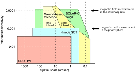
Figure 6.20: Sensitivities of different solar facilities.

The instrumentation attached to SUVIT will allow to perform precise spectroscopic and polarimetric measurements (to determine temperatures, velocities, and magnetic fields) as well as imaging of intensities and magnetic fields with high temporal cadence (to capture dynamical behaviors). A narrow-band imager is planned for polarimetric and Doppler measurements at limited number of positions in spectral lines, while a broad-band imager will provide high spatial monochromatic images of the chromosphere and the photosphere. The spectropolarimeter will reach a sensitivity of $10^{-4}$ in exposures times of $20$ s with spatial sampling of $0.2\hbox{${}^{\prime\prime}$}$ per pixel, allowing the detection of the forward scattering Hanle effect in chromospheric structures (see Fig. 6.20). It supplies a spectral sampling of $\sim 34$ mÅ at $8542$ Å ($\lambda/\Delta\lambda\sim 2\cdot 10^{5}$). Following the calculations carried out in this thesis, Solar-C should allow the first clear detection of amplifications in the linear polarization signals produced by inclined magnetic fields and chromospheric shock waves in the Ca ii transitions. As a consequence, we may have a suitable observable for capturing the dynamics and the energy transfer between the photosphere and the corona mapped by the variations of the Hanle signals.

6.5.2 Degraded and restored maps of Polarization Amplitudes.

We have applied a procedure of degradation and posterior reconstruccion to the linear polarization signals for imitating a real Solar-C observation (Figure 6.21). We followed the next steps:

• First, we calculated the total linear polarization applying Eq. (6.9) to the Stokes vector components resulting from our RT calculations, whose original spatial resolution is $\sim 0.09\hbox{${}^{\prime\prime}$}/\rm{px}$. We show the results for the $8542$ Å and the K lines in the left panels of Figure 6.21.

  $$\centering\mathrm{f_{MAX}(Q/I,U/I)}=\,100\cdot\mathrm{\sqrt{Max\left|\frac{Q}{I}\right|^{2}+Max\left|\frac{U}{I}\right|^{2}}}\quad[\%]\@add@centering$$ (6.9)

• Second, we simulate the observation with a telescope, so that we degraded the quality of the signals by convolving the original maps of I, Q and U with a spatial PSF with $\mathrm{FWHM=0.18\hbox{${}^{\prime\prime}$}}$, a spectral PSF with $\mathrm{FWHM=100\,m\AA}$, making a binning of 2 square pixels to emulate a detector pixel of $0.18\hbox{${}^{\prime\prime}$}$ (slightly lower than the pixel size in Solar-C in spectropolarimetric mode) and adding a gaussian noise that gives a sensitivity of $\mathrm{S/N=10^{4}}$ for an observation with 9 seconds of exposure time (worst case). Such operations were done in that order to imitate the real physical degradation at the satellite. With the resulting maps we calculated again the quantity of Eq. (6.9). The results are shown in the middle column panels in Figure 6.21.

• Finally, we integrated photons to improve the signal to noise ratio as if we were treating the observed signals. Thus, we averaged each 2 pixels along the x axis, doing it separately for the degraded I, Q and U maps. We preserved the pixel size avoiding binning in the operation (each pair of pixels integrated together share a common pixel with the next pair along the row). With the resulting maps we calculated again the quantity Eq. (6.9). The results are in the right column panels of Figure 6.21.

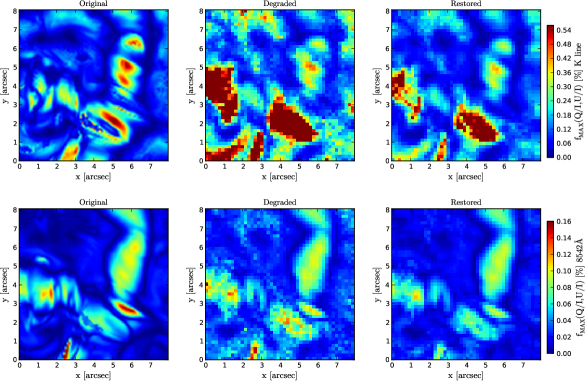
Figure 6.21: Effect of degrading and restoring the maps of maximum total linear polarization in $8542$ Å (lower panels) and K lines (upper panels). Left column: original synthetic maps. Middle column: degraded maps emulating a Solar-C observation (see text). Right colum: Recovered maps after integrating $0.36\hbox{${}^{\prime\prime}$}$ spatially along the x axis without rebinning. Each colorbar is common for a row of maps.

The first thing we note in the resulting maps are the dark red patches in the K line “observations” (Figure 6.21). They are a product of the low number of photons that we have in the emerging core intensities of this spectral line, especially in cool chromospheric areas. Such low levels of intensity in patches of cool temperatures are able to produce spurious signals much larger than the ones observed in the true maps. The pixel integration with the aim of recovering the signals is not enough to reverse that situation to acceptable levels, even when using larger pixel sizes in the integration (pixels as large as $0.5\hbox{${}^{\prime\prime}$}$ were considered) . In any case, high resolution is required to resolve the fine chromospheric structure. As a positive counterpart, we think we could use these noise patches in the K line as indicatives of a cool chromosphere. The $8542$ Å line is also susceptible of the noise in those areas but we easily recover the Hanle signals after the simple integration. However, note that the higher signal levels in strong polarization patches (red areas in the bottom left panel) are never recovered. We see here why the Doppler-induced amplifications studied in previous chapters are so elusive in the solar observations available in Ca ii. Basically, the small characteristic size and the apparently elongated shape of these highly dynamic structures avoid a coherent spatial detection. The characteristics times associated with the passage of the shock waves through the region of formation are also too short to be visible in wide areas during a single snapshot. Probably, these signatures are actually everywhere, but impossible to observe with our current instrumentation given the small spatial and temporal filling factor. In the $8542$ Å maps, we are able to restore all the LP patches in the HF region with their approximated amplitudes in most cases. We also identify the Van-Vleck HPILs in the half of the map where the horizontal field strength is larger.

6.5.3 Degraded and restored maps of the Linear Polarization Degree.

We repeated the same steps than in Section 6.5.2, but applying Ecs. (6.7):

$$\mathrm{LPD}\,[\%] =\,100\cdot\frac{\sqrt{\left[\overset{\lambda_{2}}{\underset{\lambda_{1}}{\sum}}Q\right]^{2}+\left[\overset{\lambda_{2}}{\underset{\lambda_{1}}{\sum}}U\right]^{2}}}{\overset{\lambda_{2}}{\underset{\lambda_{1}}{\sum}}I},$$

$$\mathrm{CPD}\,\left[\%\right] =\,100\cdot\frac{\overset{\lambda_{2}}{\underset{\lambda_{1}}{\sum}}|V|}{\overset{\lambda_{2}}{\underset{\lambda_{1}}{\sum}}I},$$

with the filter C ($\Delta\lambda=0.7$ Å) used in Sec. 6.3.3 to get the maps of total linear and total circular polarization degree. We have used the same instrumental parameters than in the previous section. Since these maps are the result of integrating along wavelength, their signal to noise ratio is much better and the structures and HPILs appear clearly. In all the LP degree maps, the largest amplitudes are in places with larger field strengths and insignificant velocities, and not in areas with the largest velocities as it happens in the maps of the maximum LP of Fig. 6.21. Concerning Stokes V, the spatial, spectral and noise degradation barely affects the results, making it unnecessary to sum pixels.

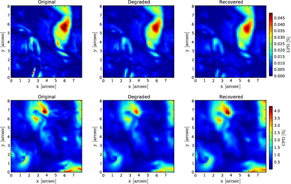
Figure 6.22: Effect of degrading and restoring the polarization degree maps using the filter C around $8542$ Å. Top row: integrated linear polarization. Bottom row: integrated circular polarization. Left column: original synthetic maps. Center column: degraded maps emulating a Solar-C observation as in Fig. 6.21 (see text).Right column: recovered maps after integrating $0.36\hbox{${}^{\prime\prime}$}$ spatially along the x axis. Each colorbar is common for a row of panels. These maps have been calculated using Eqs. (6.7a) and (6.7b).

6.5.4 The practical disadvantages of the typical spectropolarimetric quantities.

Disregarding the horizontal inhomogeneities, the only thing breaking the symmetry in a disk center observation is an inclined magnetic field. In that situation, Stokes Q and U can reach similar amplitudes irrespective of the reference for $Q>0$. Thus, to measure the total linear polarization (LP) with a single quantity, a geometrical average of Q and U is usually applied. Furthermore, it is common to use the fractional polarization, referenced to the intensity, which gives a measure that is relative to the total number of photons. Since such mathematical operations are not linear, the effect of the instrumental noise in real observations can be artificially amplified when calculating the total polarization. Then, is any of the following ways of computing the total linear polarization preferred in terms of robustness to noise?

$$\mathrm{LPD}\,[\%] =\,100\cdot\overset{\lambda_{2}}{\underset{\lambda_{1}}{\sum}}\frac{\sqrt{Q^{2}_{\lambda}+U^{2}_{\lambda}}}{I_{\lambda}}$$ (6.11a)

$$\mathrm{LPD}\,[\%] =\,100\cdot\frac{\sqrt{\left[\overset{\lambda_{2}}{\underset{\lambda_{1}}{\sum}}|Q|\right]^{2}+\left[\overset{\lambda_{2}}{\underset{\lambda_{1}}{\sum}}|U|\right]^{2}}}{\overset{\lambda_{2}}{\underset{\lambda_{1}}{\sum}}I}$$ (6.11b)

$$\mathrm{LPD}[\%] =\,100\cdot\frac{\sqrt{\overset{\lambda_{2}}{\underset{\lambda_{1}}{\sum}}Q^{2}+\overset{\lambda_{2}}{\underset{\lambda_{1}}{\sum}}U^{2}}}{\overset{\lambda_{2}}{\underset{\lambda_{1}}{\sum}}I}$$ (6.11c)

If we are interested in precisely defining the weakly polarized structures (as the Hanle polarity inversion lines defined in Sec. 6.3.2), then we need a lot of photons and consequently a quantity that adds the contributions from all the wavelengths, like the linear polarization degree (LPD). But the non-linearity of the LPD makes the way we add the different wavelength contributions important. None of the Eqs. (6.11) are valid to do it because of two reasons. First, the physical meaning of the total linear polarization has to be preserved, in such a way that the sum operations have to be applied to photons in the same polarization state, and not to combinations of them or to derived magnitudes. For instance, the sum of fractional contibutions in Eq.(6.11a) has not the same physical meaning that the concept of “fractional polarization” in the sense it is not referenced to a maximum value of $100\%$. And second, considering measures with gaussian noise (e.g., Q), their derived unsigned quantities (e.g., $Q^{2}$ or $|Q|$) have Rayleigh noise. When summing the Rayleigh contributions for each wavelength, the noise is added and not cancelled out (as in the gaussian case). Then, Eqs. (6.11b) and (6.11c) are not valid either.

The remaining basic solution would be the Eq. (6.7). However, it has the disadvantage of suffering from signal cancellations in lines whose profiles have mixed polarities, as it can happen with the antisymmetric profiles produced by the velocity gradients in the LP signals of the $8498$ Å line. Other disadvantage is the dependence of Eq. (6.7) on the passband chosen to perform the integration (see Sec. 6.3.3). This is because it tends to zero as the bandwidth is enlarged, instead of tending to a fixed value proper from the LP in the line.

On the contrary, in order to capture the effects of dynamics in the polarization amplitudes, we need quasi-monochromatic quantities. In that case, the polarization maps of Q$/$I and U$/$I should be calculated at the wavelengths of the maximum amplitudes at each pixel, which also gives a better signal-to-noise ratio. If we use the line center wavelength, the polarization amplitudes will appear decreased in map areas with chromospheric motions, avoiding the detection of dynamic amplification effects on the LP.

The quantity we chose to calculate Fig. (6.21) is given by Eq. (6.9). The polarization patches in the “restored” map (right panel) of the figure are a product of the noise in the faint core intensity emerging from cool- chromospheric areas. There, the LP is usually larger and the intensity is minimum, making the unstable quotients of Eq. (6.9) to diverge. A possible solution is using the median (instead of the max function) to define the measure:

$$\centering\mathrm{f_{MEDIAN}(Q/I,U/I)}=\,100\cdot\mathrm{\sqrt{\left[{Median}\left|Q/I\right|\right]^{2}+\left[{Median}\left|U/I\right|\right]^{2}}}\quad[\%],\@add@centering$$ (6.12)

where the medians are calculated in a small passband ($\Delta\lambda_{\rm med}$) of a few wavelength points chosen around the common maximum for Q and U. Since the median of several points around the maximum is less affected by high- frequency excursions due to the noise, it estabilizes the results without loosing the signal information at the maximum. Using three points of bandwitdh as the best choice, we got the maps of Fig. (6.23). To calculate them, we repeated similar steps than in Sec. (6.5.2), with the same instrumental parameters, but applying Eq. (6.12).

In the case of the $8542$ Å map (lower panels in Fig. 6.23), the result of using the median is perhaps a bit better than using the maximum value (lower panels in Fig. 6.21) because we obtain a slightly better contrast in areas with low polarization levels and recovered amplitudes that are more similarto the ones in the original map. For the K line (upper panels of the same figures), the results are also a bit better, but still unsatisfactory to distinguish between the signal and the noise in cool areas.

Increasing the level of noise one order of magnitude ($\rm{S/N=10^{3}}$), we do not get images with good quality for any line (see Fig. 6.24 and A.6) or any method. In the more favorable case of the $8542$ Å line, even the LPD does not allow us to distinguish the signals from the noise in a large area of the map (lower right panel in Fig. 6.24). We would need to integrate more in time or space, so losing the required resolution and the possibility of capturing the fast and small chromospheric events.

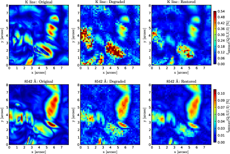
Figure 6.23: Effect of using the median (following Eq. 6.12) instead of the maximum value for calculating the total LP amplitudes in synthetic observations. Upper row: polarization amplitudes for the K line. Lower row: polarization amplitudes for the $8542$ Å line. To be compared with Fig. 6.21.

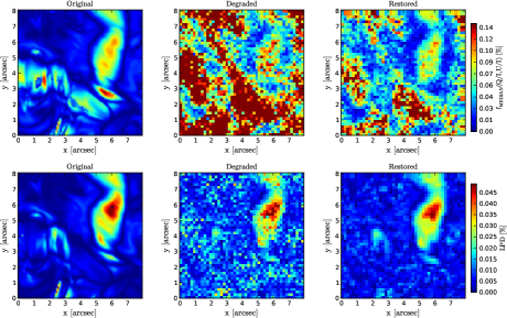
Figure 6.24: Synthetic observational maps of the $8542$ Å line, assuming a $\mathrm{S/N=10^{3}}$ in the detector. Upper row: Linear polarization amplitudes calculated using the median with Eq. (6.12). Lower row: Linear polarization degree calculated following Eq. (6.7a). The degradation and restoration process followed from column to column is the same as in previous figures, but with $\mathrm{S/N=10^{3}}$.

6.5.5 Reconstruction with PCA methods.

We have seen that the instrumental noise can easily prevent the detection of the chromospheric linear polarization (LP) features in the Ca ii IR triplet lines. In the past, Principal Component Analysis (PCA) has demostrated to be effective in denoising maps of Stokes profiles with much lower resolution than the ones that the Solar-C satellite and the future instrumentation will produce (Rees et al., 2000). It can be useful when the method is applied to a large set of correlated signals (e.g., Stokes profiles in a map) that are masked by uncorrelated spurious signals (e.g., Gaussian noise). In this section, we evaluate the application of PCA to our synthetic observations of the LP in order to find out whether it is possible to effectively clean them from the noise. We experiment with two different strategies.

In the first strategy, we obtain the PCA basis with the theoretical database of scattering polarization signals resulting from our RT calculations in the weak field regime. Our working assumption is that they can be used to explain high-sensitivity observations of the solar chromosphere as well as to validate the physical model adopted in our calculations. Later on, we use this basis to filter the noise in our synthetic observations.

Thus, we focus on two datasets of profiles for the $8542$ Å line: the dataset $1$ contains only half of the Stokes Q map calculated from the MHD models; the dataset $2$ contains all the synthetic profiles in the Stokes U and Stokes Q maps after degrading them to mimick a Solar-C observation (as we did in previous sections). We use the dataset $1$ (i.e., the well-resolved non-degraded original profiles) as the initial PCA database . Selecting only a half of the map in Stokes Q to build the database, we can see if it is enough to explain other regions in the map and also the Stokes U signals. This database has $4185$ profiles.

We use our codes (see Section 3.3) to calculate the PCA basis from the profiles database. We obtain a set of $5$ eigenvectors, which explain $99,69\%$ of the variance of the dataset $1$. Next, we project the “measured” profiles (dataset $2$) into the basis formed by the first $3$ eigenvectors (the more representative ones) and we reconstruct the Q and U signals with them. We repeat the procedure for the intensity and we use the outputs to calculate the maximum linear polarization with Eq. (6.9). The results, comparing the original synthetic map with the PCA-reconstructed one, are shown in Figure 6.25.

Figure 6.25: Simulation of the observational degradation in the maximum LP (middle panel) and its reconstruction with PCA (right panel). The detection parameters are the same as in Fig. 6.21. The PCA reconstruction have been done independently in each Stokes parameter.

In similar circunstances, the reconstructed map is cleaner and more precise than any other one shown in the previous sections. We also obtain a clear reconstruction of the more significant amplitudes in the individual Stokes parameters, with very small noise variability from pixel to pixel (see Figure 6.26). Contrarily, the maximum linear polarization, although good, still presents noisy variability. This means that, despite the effective PCA cleaning done in each Stokes parameter, the non-linear combination of them in fractional quantities still induces imprecisions in the amplitudes. The application of PCA directly to a fractional quantity, $Q/I$ for instance, does not fix the problem because the noise is still amplified before correcting it. In that case, the reconstructed maps are worse. We remark that the PCA treatment on individual Stokes parameters also shows a correct discrimination of the sign of the LP profiles in most pixels (Figure 6.26), which is relevant to our discussion about the orientation of the magnetic field (see Table 6.1).

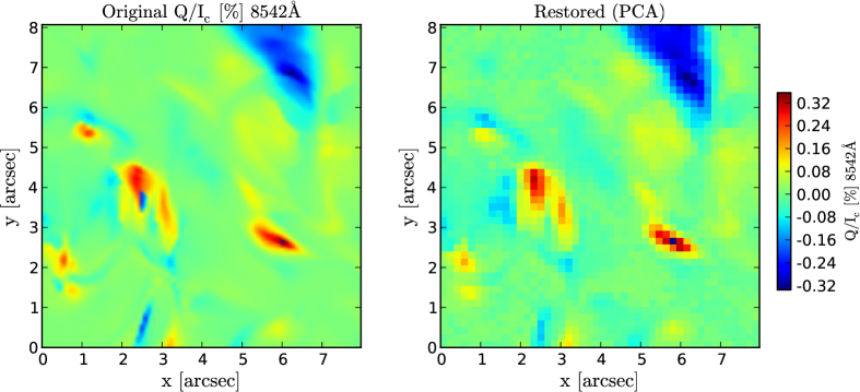
Figure 6.26: Maps of maximum $Q$ amplitudes at $8542$ Å (including sign and normalized to the continuum intensity $I_{c}$) that illustrate the result of applying PCA to denoise a synthetic Solar-C observation. Left: original synthetic map. Right: Recovered map after applying PCA to the corresponding degraded map (not shown). We assumed the same instrumental parameters than in Fig. 6.21, including a S/N ratio of $10^{4}$ in the detector.

The signs discrimination is done from just an approximated reconstruction with regular fits to the signal shapes, as illustrated by Figure 6.27. In it, we can see the specific shape of the profiles and compare different stages during the signal processing. It is interesting to note the combined effect of the spectral, spatial and thermal degradation in the profiles (compare blue and black lines in Fig. 6.27) and the effect of applying PCA (red profiles in the same figure). Note that the blue profiles can never be obtained because they represent the ideal case before detection.

Our second PCA experiment consists of generating the database from the noisy synthetic observations, which are emulated from the synthetic profiles (current spectropolarimetric observations still lacks resolution and sensitivity). The procedure is similar than before. We have also used half of the map in Stokes Q (now degraded) to build the database. The result is that the so-obtained “observational” PCA basis also permits a similarly good signal reconstruction that matches acceptably with the original amplitudes. The PCA basis contains noise in the first eigenvectors, which is normal because our database is finite. Despite of that, from Figure 6.28 we conclude that both strategies to create the PCA basis give a similar accuracy to reconstruct the maximum amplitudes. The use of a theoretical non-degraded database (first strategy) has been however better to fit the profile shapes and to obtain a more accurate LP sign in the reconstructions.

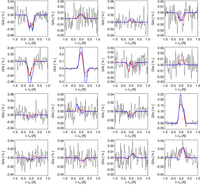
Figure 6.27: Examples of profiles at random pixels in the degraded observational map. In black, the Solar-C “observation”, in red the PCA reconstruction. In blue, the real profiles that would be captured by a Solar-C pixel without introducing any instrumental degration.

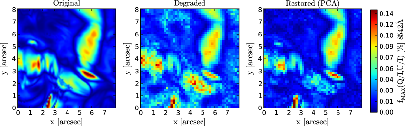
Figure 6.28: The same as Figure 6.25, but using a PCA database formed by synthetic observations instead of by non-degraded theoretical profiles.

PCA seems to be able to model variable and asymmetric profiles resulting from dynamic solar models. For this conclusion to be extended to real observations when using a theoretical PCA basis, it has to be proved that our physical model is a good representation of reality. It is then necessary to have a sufficiently large number of pixels covering most of the possible physical circumstances in the atmosphere. As the dynamics introduces more degrees of freedom, we expect such initial database to be larger than in the static case. On the other hand, for PCA to be useful in dynamic circumstances when using a true observational database, the number of observations has to be large enough for the noise in the first eigenvectors of the basis to tend to zero.

Although PCA is not much better than the mere spatial integration to reconstruct the fractional polarization profiles, it gives the best results while simultaneously maintaining the spatial and temporal resolution of the dataset. Furthermore, it seems to assure a good fit to the LP signs and amplitudes. PCA provides a promising way of testing the physical models adopted in our calculations just by projecting a high-quality chromospheric observation into our theoretical PCA basis, which offers a simple feedback for the development of MHD models and the physics of polarization. Our study can be a useful anticipation for treating the analysis of well-resolved dynamic observations that the future solar facilities will provide.

6.6 Spectropolarimetric inference of the magnetic field.

In this section, we use the Hanle and Zeeman effect for trying to deduce as much information as possible about the orientation, inclination and strength of the magnetic field in our synthetic quiet regions at disk center. The aim is to show some issues relevant to the inference process in the Hanle regime and how the thermodynamics and dynamism of the atmospheric plasma may affect this inference problem.

Determinations of the vector magnetic field in the solar atmosphere are essential for understanding solar magnetic structures in general, and specifically for quantifying or even predicting solar activity. Vector magnetic fields are inferred from the Stokes parameters, I, Q, U, and V (e.g., see Socas-Navarro et al., 2000; Asensio Ramos et al., 2008). However, the component of the field that is perpendicular to the line of sight (transverse component), as inferred from observations of linear polarization produced by the Zeeman effect in magnetically sensitive spectral lines, has an inherent $180\,\mbox{${}^{\circ}$}$ ambiguity in its azimuth (Unno, 1956). To fully determine the transverse component of solar vector magnetograms inferred by the Zeeman effect, this ambiguity must be resolved.

Calculation of electric currents, magnetic energy and helicity budgets and most techniques of coronal magnetic field extrapolation rely on disambiguated vector magnetograms. The azimuth ambiguity (e.g., Harvey, 1969) continues to be an open research topic today. Nowadays, vector magnetograms are routinely provided by the ground-based Vector SpectroMagnetograph (VSM; Henney et al., 2009) of the Synoptic Optical Long Term Investigations of the Sun (SOLIS) facility (Keller et al., 2003) and by the space-based SpectroPolarimeter of the Solar Optical Telescope (SOT Tsuneta et al., 2008) onboard the Hinode spacecraft. Vast amounts of seeing-free full-disk vector magnetograms are also delivered by the Helioseismic and Magnetic Imager (HMI Scherrer et al., 2012) on board the Solar Dynamics Observatory (SDO) mission.

Having these facilities, numerous efforts have been made toward solving the $180\,\mbox{${}^{\circ}$}$ ambiguity problem of the Zeeman polarization signals. There is no known method for resolving the ambiguity through direct observation using the Zeeman effect. Hence, to resolve the ambiguity, some further assumption on the nature of the solar magnetic field must be made. Typical assumptions focus on the spatial smoothness of the field or on minimizing the divergence of the field. A number of different algorithms have been developed to resolve the ambiguity, each making various assumptions on the character of the solar magnetic field.

For magnetograms obtained with photospheric or chromospheric lines (Leka & Metcalf, 2003) azimuth disambiguation is not a trivial problem problem because the height derivatives ($\partial/\partial z$) of most of the parameters are needed but unknown. While tackling this problem, methods have evolved gradually from a simple comparison between observed and extrapolated fields to computerized automatic procedures. These methods can be classified as “reference field” (Allen Gary & Hagyard, 1990), “multistep process” (Moon et al., 2003), “interactive”, such as the AZAM utility (Metcalf et al., 2006a), “automated minimization” (Metcalf, 1994), “vertical current minimization” (Georgoulis, 2005), “noniterative analytical” (Skumanich & Semel, 1996; Cuperman et al., 1993), and “spectroscopic” (Landi Degl’Innocenti & Bommier, 1993), this last one being inapplicable for disk-center and limb observations. Except for the spectroscopic method and the non-iterative analytical methods by Cuperman et al. (1993) that were tested with a MHD model, all the other methods are routinely applied to observational data by individual researchers. Some years ago, Metcalf et al. (2006b) provided an overview of nearly all existing algorithms for resolving the $180\,\mbox{${}^{\circ}$}$ ambiguity problem when applied to synthetic data at a single height level.

The assumptions underlying each method are the ones ultimately responsible for the quality of the disambiguation results. Precisely and self-consistently disambiguating a vector magnetogram is a challenging problem, especially when considering complex magnetic structures with a multipolar, stressed, and sheared photospheric boundary. For that reason, the application of a proper authomatized disambiguation procedure and the practical issues deriving from the previously commented techniques are out of the scope of this work.

We restrict this section to clarify and illustrate some new results of this problem in the case the linear polarization is dominated by scattering processes and the Hanle effect, which is suitable for studying quiet regions of the Sun. The dependence of the linear polarization on the magnetic field azimuth is governed by the Hanle effect, but we show how the thermodynamic alters the inference, making the problem more complicated but more interesting. We focus on disk-center observations and highly-resolved quiet regions of the chromosphere by using the polarization of the Ca ii IR triplet lines we have calculated in the 3D MHD model. The use of these spectral lines may give us information about the three-dimensional topology of the chromospheric magnetic field.

6.6.1 The Zeeman effect and the weak field approximation.

A useful observable to infer information on the longitudinal component of the magnetic field is the Stokes V profile produced by the Zeeman effect. In the weak field regime, the Zeeman splitting ($\bar{g}\Delta\lambda_{B}$, with $\bar{g}$ the effective Landé factor ) is small in comparison with the thermal width ($\Delta\nu_{D}$) of the line profiles (see Sec. 2.1.3):

$$\centering\bar{g}\cdot\frac{\Delta\lambda_{B}}{\Delta\nu_{D}}\,=\,\bar{g}\cdot\frac{1.4\cdot 10^{-7}\,\lambda_{0}[\mathrm{\AA}]\,B[G]}{\sqrt{1.663\cdot 10^{-2}\frac{T[K]}{m[\mathrm{u.m.a.}]}+v_{\rm micro}^{2}[\mathrm{km^{2}s^{-2}}]}}\ll 1,\@add@centering$$ (6.13)

with $m=40.06$ u.m.a for calcium. The condition (6.13) is fulfilled at all the heights where the lines form in our models. In the weak-field regime, and assuming the absence of atomic orientation and that the longitudinal magnetic field component is constant along the formation region, we can approximate Stokes V at disk center with:

$$V(\lambda)\,=\,-\bar{g}\,\Delta\lambda_{B}\,\cos{\theta_{B}}\,\frac{\partial I(\lambda)}{\partial\lambda},$$ (6.14)

where $\theta_{B}$ is the inclination of the magnetic field with respect to the LOS and $I(\lambda)$ gives the spectral profile of the emergent intensity. Note that, assuming a LOS with $\mu=1$, a line in absorption under a magnetic field with $0\,\mbox{${}^{\circ}$}<\theta_{B}<90\,\mbox{${}^{\circ}$}$ gives a Stokes V profile that is antisymmetric with a positive lobe at blue wavelengths and a negative one towards the red. The sign of the lobes will be the opposite when the magnetic field points away from the observer or the line is in emission. Since $\Delta\lambda_{B}$ is linear in B, Stokes V is proportional to the longitudinal component of the magnetic field.

Taking into account the discussion about that HPILs in Section 6.3.2, we can use the regions of null linear polarization across a map to distinguish the lines where the magnetic field has an exact inclination $\theta_{B}=54.73\,\mbox{${}^{\circ}$}$ (Van-Vleck HPILs).

6.6.2 Magnetic Field Direction and Ambiguities in the Hanle regime.

In order to estimate the magnetic field azimuth it is necessary to apply Eq. (6.2). However, the inverse tangent is only defined from $0\,\mbox{${}^{\circ}$}$ to $90\,\mbox{${}^{\circ}$}$ when applied to positive angles measured from the x axis of Fig. 6.11. This is called the inverse tangent problem, because it is not directly possible to recover an angle between 0 and 360 degrees from the ratio between the two spatial vector components defining a direction in the plane $(x,y)$. That is exactly what we seek when applying Eq. (6.2) to obtain the magnetic field azimuth. The problem results in the appearance of two ambiguities in the magnetic field azimuth: the $90\,\mbox{${}^{\circ}$}$ ambiguity is produced when an azimuth $\chi_{B}$ gives a ratio U/Q undistinguishable from the one given by $\chi^{\prime}_{B}\pm 90\,\mbox{${}^{\circ}$}$; and the $180\,\mbox{${}^{\circ}$}$ ambiguity is produced when an azimuth $\chi_{B}$ gives a ratio U/Q undistinguishable from the one given by $\chi^{\prime}_{B}\pm 180\,\mbox{${}^{\circ}$}$. To solve the $90\,\mbox{${}^{\circ}$}$ ambiguity we need the specific signs of each component (Q and U), and not only the ratio. Thus, the calculation of the azimuth depends on such signs as follows:

$Q$	$U$	$2\,\chi_{B}$
$+$	$+$	$\tan^{-1}{|U/Q|}$
$+$	$-$	$\pi-\tan^{-1}{|U/Q|}$
$-$	$+$	$\pi+\tan^{-1}{|U/Q|}$
$-$	$-$	$2\pi-\tan^{-1}{|U/Q|}$

Table 6.2: Signs rule to solve the Eq.(6.2).

Whenever the signs of Q and U do not change by other factors different than the magnetic field azimuth (basically field inclination and thermodynamics) or whenever we can trace such changes back, the $90\,\mbox{${}^{\circ}$}$ ambiguity can be solved. However, as the argument of the tangent in Eq.(6.2) is $2\chi_{B}$ (and not $\chi_{B}$), this procedure cannot solve the $180\,\mbox{${}^{\circ}$}$ ambiguity. This is because the light, being an electromagnetic wave, oscillates in both senses along its direction of polarization in such a way that the information about the magnetic field orientation is missed. To deduce it, we should recall all the methods and the problematic around the resolution of this ambiguity. However, the sense of the chromospheric magnetic field can also be determined with the magnetic polarities at both ends of the magnetic field lines crossing the pixel of interest. To obtain such field lines we need to consider a map (not only one pixel) and the sign of Stokes V. We have to identify the field line crossing each pixel, just by calculating the transverse field directions given by Eq. (6.2) and connecting them between adjacent pixels from a positive polarity region (Stokes V with positive blue lobe and negative red lobe) to a negative polarity region (Stokes V with opposite sign) or viceversa. We do not see major impediments in doing this, at least in our dataset, where we deal with smooth chromospheric structures with no significant noise added. With such topological procedure we could solve the $180\,\mbox{${}^{\circ}$}$ ambiguity.

The application of Table 6.2 to our LP signals has some crucial remarks that have to be clarified. In order to solve the correct azimuth, we have to know the Q and U signs. Since they do not only depend on the magnetic field azimuth, we have first to discriminate all the elements (drivers) acting on the polarities and deduce the signs that would be given only by the magnetic field orientation. Considering a Hanle-saturated spectral line and a forward scattering gemetry, the possible drivers are:

1) The term $(3\cos^{2}{\theta_{B}}-1)$ depending on the inclination of the magnetic field with respect to the vertical in Eqs. (6.4). It contributes with negative sign to both Q and U when the pixel is in the HF region (when the inclination is $54.73\,\mbox{${}^{\circ}$}<\theta_{B}<125.27\,\mbox{${}^{\circ}$}$). That makes the signs for (Q,U) in Fig. 6.11 to jump together between states: $(++)\leftrightarrows(--)$ or $(+,-)\leftrightarrows(-,+)$. The effect is always a sudden $90\,\mbox{${}^{\circ}$}$ shift in the inferred azimuth angle when crossing the Van Vleck HPILs (when passing from the HF to the VF region or viceversa). This is usually called Hanle ambiguity, and affects the inferred magnetic azimuth due to the magnetic inclination. We can avoid it by two means. First, with the above-mentioned topological method. This is, using the circular polarization in a map as a marker to discriminate the correct magnetic field direction between the two ambiguous perpendicular magnetic field azimuths. Second, using only one pixel, but knowing the theoretical reference sign (see Table 6.1) for the model that better represents that pixel and discriminating the drivers affecting it.

2) The temperature. To account for it, we classify the models in simple categories: FALC-like, cooler, hotter and so on. Thus, we associate the specific states of the linear polarization with those general macroscopical states (again Table 6.1). Once we know the theoretical behaviour of the polarization signs in a range of temperatures, we can use that information as a reference. In this case we need to know the sign of the thermodynamic factor $\mathcal{F}$ in static cases.

3) The velocity gradients. We concluded in Section 6.4 that the velocity could affect the LP signs in the Sun or in more dynamic models, but not in our MHD models. In any case, the existence of a velocity gradient does not produce just a sign reverse and a discrete azimuth jump as it happens with the variation of the magnetic field inclination. Instead, it induces gradual alterations of the Q and U amplitudes that are translated in imprecisions when estimating the magnetic field azimuth with Eq. (6.2). Only when the velocity gradient overcome a certain threshold, such gradual change also leads to a reversal in the linear polarization (e.g., see Fig. 5.8). That was a common behavior for the $8498$ Å line forming in the time-dependent models of Chapter 5. On the contrary, the lines $8542$ and $8662$ Å are unable to change their signs when they have a one-peak shape because in that case the velocity gradient always produces a positive amplification (Chapter 4). Instead, if they show a valley shape at line center, a change of polarity is possible due to the contribution of the lower level alignment producing the valley.

Our discussion on the ambiguities focuses on the saturated Hanle regime under the weak field approximation. If the field is stronger, the transverse Zeeman effect signals predominates as the sources of the linear polarization (Zeeman regime). On the contrary, if the field is on the order of a few gauss weaker, the Hanle polarization amplitudes in these lines can vary significantly with the magnetic field strength and introduce a different angular dependence in the equations.

Ambiguities in inclination with ambiguous azimuth.

The previous explanations introduce the ambiguities in azimuth without specifying the corresponding values of magnetic field inclination that can produce the same Q and U. To do that, we pose the problem in a more analytical way as follows.

The lack of knowledge about the azimuth and the inclination of the magnetic field produces spectroscopic ambiguities. It means that different magnetic field orientations yield the same Q and U, making the field topology undistinguishible. To see the exact magnetic field configurations that can be mixed up, let us consider a fixed thermodynamical stratification and answer the following question: which two different magnetic field orientations, $(\chi_{B},\theta_{B})$ and $(\chi^{\prime}_{B},\theta^{\prime}_{B})$, are undistinguishable when only Stokes Q and U are used to infer them?

Considering that the angular depedencies of the Stokes U profile are well described by Eq. (6.4b), the answer to the question can be obtained making $U=U^{\prime}$. It yields

$$\centering\sin{2\chi_{B}}\cdot\sin^{2}{(\theta_{B})}\cdot(3\cos^{2}{\theta_{B}}-1)=\,\sin{2\chi^{\prime}_{B}}\cdot\sin^{2}{(\theta^{\prime}_{B})}\cdot(3\cos^{2}{\theta^{\prime}_{B}}-1).\@add@centering$$ (6.15)

The ambiguities in inclination are associated with the existent ambiguities in azimuth. Thus, for the azimuthal $180\,\mbox{${}^{\circ}$}$ ambiguity, the corresponding ambiguous inclinations $\theta_{B}$ and $\theta^{\prime}_{B}$ are obtained when $\chi_{B}=\chi^{\prime}_{B}+180\,\mbox{${}^{\circ}$}$ is substituted in Eq. (6.15). Note it gives the same as when the azimuth is considered as solved and fixed ($\chi_{B}=\chi^{\prime}_{B}$), indicating that both situations are spectroscopically equivalent. Then, it yields:

$$\centering\sin^{2}{(\theta_{B})}\cdot(3\cos^{2}{\theta_{B}}-1)=\,\sin^{2}{(\theta^{\prime}_{B})}\cdot(3\cos^{2}{\theta^{\prime}_{B}}-1),\@add@centering$$ (6.16)

whose solutions give the relations between the ambiguous inclinations $\theta_{B}$ and $\theta^{\prime}_{B}$:

$$\theta_{B}=\cos^{-1}\left[\pm\sqrt{\frac{2}{3}\pm\sqrt{\frac{1}{9}+\sin^{2}{\theta^{\prime}_{B}}(\cos^{2}(\theta_{B}^{\prime})-1/3)}}\right]$$ (6.17)

The same reasoning and results are obtained using Q. These solutions ($180\,\mbox{${}^{\circ}$}$ ambiguity case or solved azimuth case) are represented by the black curves in Fig. 6.29. Thus, a value $\theta^{\prime}_{B}$ (vertical axis in Fig. 6.29) can produce the same U (and Q) than other inclinations $\theta_{B}$ (horizontal axis), which are obtained by tracing a horizontal line that crosses in several points the black curve. We see that a value lying in the HF region (coloured region in Fig. 6.29) does not have ambiguities (does not cross any curve) in the range $63.77\,\mbox{${}^{\circ}$}<\theta_{B}<116.23\,\mbox{${}^{\circ}$}$. That means that near-horizontal fields in that range of inclinations produce ambiguities only due to azimuth and/or thermodynamics, so highlighting the HF areas as the preferred ones to be used for estimating inclinations from Q and U. If the inclination is out that range but still in the coloured region, a horizontal line in the figure yields four ambiguities, two at a right branch and two at a left branch. Finally, if the inclination is in the VF region (white area), there are only two ambiguities, one at each branch.

In the case of an azimuth $\chi_{B}$ not distinguished from $\chi_{B}\pm 90\,\mbox{${}^{\circ}$}$ (Hanle ambiguity), Eq. (6.15) changes to:

$$\centering\sin^{2}{\theta_{B}}\cdot(3\cos^{2}{\theta_{B}}-1)=\,-\sin^{2}{\theta^{\prime}_{B}}\cdot(3\cos^{2}{\theta^{\prime}_{B}}-1),\@add@centering$$ (6.18)

whose solutions are the same as Eq. (6.17) but with a minus sign after the number $1/9$:

$$\centering\theta_{B}=\cos^{-1}{\left[\pm\sqrt{\frac{2}{3}\pm\sqrt{\frac{1}{9}-\sin^{2}{\theta^{\prime}_{B}}(\cos^{2}(\theta_{B}^{\prime})-1/3)}}\right]}\@add@centering$$ (6.19)

The new solutions are represented by the blue curves in Fig 6.29. Thus, under this azimuthal ambiguity, the inclination $\theta^{\prime}_{B}$ (vertical axis) is also ambiguous because it cannot be distinguished from $\theta_{B}$, but now it is only true in the VF region because the blue curves do not exist outside of it.

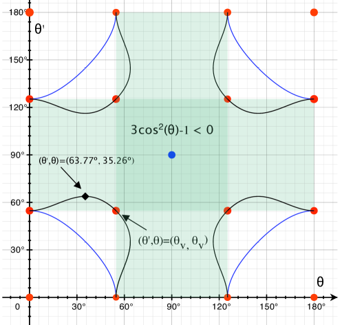
Figure 6.29: Theoretical curves leading to an ambiguous magnetic field inclination in the saturated Hanle effect at forward scattering. The green shadowed region is the HF region, where $3\cdot\cos^{2}{\theta_{B}}-1<0$. The relevant angles are $\theta=90\,\mbox{${}^{\circ}$}\pm 26.22\,\mbox{${}^{\circ}$},\,90\,\mbox{${}^{\circ}$}\pm 35.27\,\mbox{${}^{\circ}$}$ and $90\,\mbox{${}^{\circ}$}\pm 90\,\mbox{${}^{\circ}$})$.

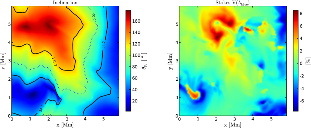
Figure 6.30: Left: inclination of the magnetic field at heights with $\tau^{8662}=1$. Right: Blue lobe amplitude of Stokes V, indicating the direction of the longitudinal magnetic field component (blue is magnetic field vector towards the observer).

When the $90\,\mbox{${}^{\circ}$}$ ambiguity in azimuth is not solved, the black and the blue curves together give all the ambiguities in inclination. When the $90\,\mbox{${}^{\circ}$}$ ambiguity is solved (using Table 6.1), the “blue solutions” do not hold and only the “black ones” leave. In that case, the remaining ambiguities in inclination could be eliminated with just knowing if the pixel is in the HF region or not. The reason is that the black curves always connect inclinations $\theta^{\prime}_{B}$ in the HF region with inclinations $\theta_{B}$ in the VF region and viceversa. In other words, if the pixel is clearly in one region (VF or HF), the magnetic field inclination in that pixel cannot pertain to the other region. In practice, to take advantage of that, the division between the HF and VF regions has to be located by identifying the Van-Vleck HPILs, which can be easily done calculating the degree of total polarization (see Figure 6.14).

The above discrimination is not valid in the blue curves because they connect inclinations in the same area. We would need to divide the VF region in more subregions to avoid ambiguities. Indeed, if we were able to identify other inclination ranges spectroscopically (having acces to other LOS, for example) we could repeat this strategy of segmentation to differentiate other inclinations and then fit inclination curves between $0$ and $90\,\mbox{${}^{\circ}$}$ in further steps.

Note that the mere fact of interpreting the results in a map give some extra help to solve the ambiguities. We can use physical methods as the ones introduced by other authors or use topological arguments (connecting azimuth field lines, identifying regions in a map) together with spectroscopical measurements (HPILs, signs of V, Q and U, value of $\rm{U/Q}$). Without the Van-Vleck HPILs and the Stokes V profiles, the magnetic field inclination can never be univocally obtained from Q and U.

In conclusion, the calculation of the magnetic field azimuth depends on the LP signs that are modified mostly by the temperature and the field inclination. Knowing the temperature regime (cool or hot), we only need to identify the Van-Vleck HPILs separating inclination regions (VF or HF) to get the correct azimuths with Table 6.2. At the same time, the distinction of those regions eliminates the $90\,\mbox{${}^{\circ}$}$ ambiguities in azimuth and the corresponding ambiguities in inclination (blue curves, Fig. 6.29), leaving only the $180\,\mbox{${}^{\circ}$}$ ambiguity in azimuth and selecting the correct inclination as the one pertaining to the region in which the pixels is. To know if the field is pointing towards or away the observer (which is equivalent to select between right or left branches in Fig. 6.29) we can use the polarity of Stokes V in the pixel. Finally, to know the sense of the magnetic field vector we estimate possible to solve the $180\,\mbox{${}^{\circ}$}$ ambiguity in azimuth using a topological method based in connecting all the field lines from positive to negative magnetic emergence patches (Fig. 6.30). In any case, we remark that in a wide inner part of the HF region the azimuths are unaffected by inclinations, and inclinations itself do not show any ambiguity. All the discussion is based on that we can discriminate the non-magnetic factors altering the polarity signs, which have been presented after theoretically calculating the reference polarities in realistic maps of the solar chromopshere.

6.6.3 The disambiguation process.

We have provided some ideas for deducing the general topology of the magnetic field. Now, we want to get the map of the magnetic field azimuth without ambiguity. To do it, we will explain the map of magnetic field azimuth in Figure 6.31 and the steps followed to create it. These steps are based only on the information provided by the “observed” Stokes vector.

1) The first thing we need are the maps of maximum Stokes Q and U at each pixel for a Hanle saturated spectral line (both $8662$ and $8542$ Å lines are good options). In order to apply Eq. (6.2) and estimate the field azimuth, some authors (e.g. Jefferies et al., 1989) integrate the spectral profiles of Q and U along a certain filter width. However, the most precise way of inferring the magnetic field azimuth at optical depth unity is to consider the narrowest spectral width possible, ideally only at the wavelength where the Stokes Q and U amplitudes are maximum. If not, we will mix contributions coming from different layers or we will produce signal cancellations due to asymmetric profiles induced by velocity gradients. The central line wavelength is not a good choice because the resulting spatial maps would show some empty patches in the atmospheric regions where the velocity gradients are considerable.

2) Following table 6.2, we calculate the azimuth of the magnetic field. But that is not the final azimuth because we have first to consider other factors affecting the signs of Q and U. Note that in Fig. 6.31 the original magnetic field direction (blue segments) and the azimuth calculated from Q and U exclusively (red segments) are equally oriented in many patches but they differ in a non-negligible part of the map (obviously, where the red segments are visible). Most of those wrong red segments are rotated $90\,\mbox{${}^{\circ}$}$ from the correct directions. The reason of this almost exact and discrete shift is that either the temperature stratification or the magnetic field inclination or both at the same time are modifying the signs of both Q and U (see Sec. 6.6.2). If we perfom a $90\,\mbox{${}^{\circ}$}$ rotation in the red segments, the map is almost entirely correct. Thus, the major problem to calculate the precise magnetic azimuth in those pixels is the LP sign, not the amplitudes.

3) The next step is to identify the Van-Vleck HPILs in the maps of total linear polarization (Fig. 6.13) or in the maps of linear polarization degree (Fig. 6.14). With these lines (gray lines in Fig. 6.31) we separate with precision the HF region (strip of null Stokes V in Fig. 6.13) from the VF region (coinciding with intense Stokes V in Fig. 6.13).

4) Since we know that the magnetic field lines go from the negative flux regions (blue areas in right panel of Fig. 6.30) to the positive ones around $(x,y)=(2,5)$, the correct direction of the segments can be identified just connecting them from one polarity to the other. This argument of contuinity constitutes a topological inference method that can be automatized. At least, it seems feasible for our chromospheric synthetic results.

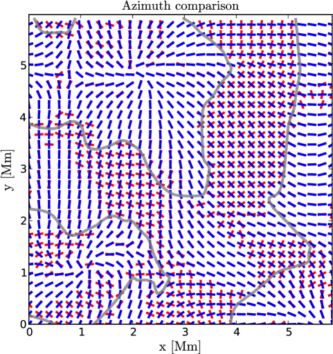
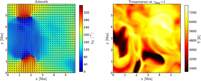
Figure 6.31: Effect of the temperature, magnetic field and dynamics on a diagnostic map in saturated Hanle regime and forward scattering. Upper panel: Comparisson between real and calculated magnetic field azimuth. Dark blue segments indicate the real direction of the magnetic field in the model at $\tau^{8662}=1$. The red segments are the same but calculated from Q and U. Gray solid iso-contours are the Van-Vleck HPILs and connect points with $\theta_{B}=\theta_{V}$ and $\theta_{B}=\pi-\theta_{V}$. Lower left panel:Original magnetic field azimuth at $\tau^{8662}=1$ in the snapshot. Lower right panel: temperature at $\tau_{8662}=1$.

For spectral lines forming in the chaotic photosphere it would be unsuitable because the derivatives of the magnetic field with height are larger.

5) As we have been introducing in previous sections, other way of inferring the correct direction for the red segments is by using reference signs for Stokes Q and U. The simplest way to do it is by identifying a patch inside the HF region in Fig. 6.15 whose linear polarization signal is mostly in Q or in U and whose thermodynamical stratification can be catalogued as one of the column cases in the Table 6.1. The example we put in the previous section was the U patch around $(x,y)=(4.5,4)$ Mm. It is a good option because the corresponding intensity map is in emission there (Fig. 6.10 at $(x,y)=(5.5,6.5)$ arcsec), so it is a model with a clear hot temperature stratification, and has almost null Q signal. Then, looking the corresponding contrast map (Fig. 6.15), we see that $U>0$. As indicated by the third column and fourth row in Table 6.1, it is compatible with a magnetic field along the $-$U axis. So, the red segments corresponding to that patch in Fig. 6.31 are wrong due to the temperature and have to be rotated $90\,\mbox{${}^{\circ}$}$. A similar inference can be done when both Q and U are not zero, just searching the projections of the magnetic field vector on the reference axes of Figure 6.11 and applying Table 6.1. This is also a procedure that can be automatized.

6) Once we know the correct azimuth directions in only one patch (reference patch) we can deduce others from it. Different regions appear clearly differenciated around such reference patch when the inclinations jumps between HF and VF regions or when the thermodynamic structure changes significatively. Thus, moving in the HF region, the patches adjacent to the reference patch appear necessarily only when having a very different kind of temperature stratification. If the reference patch has a FALC-like (or hotter) structure, the adjacent patch has to be cool, what means a simultaneous sign reversal in Q and U, and consequently a $90\,\mbox{${}^{\circ}$}$ shift in the azimuth. As a reference FALC-like patch already has a $90\,\mbox{${}^{\circ}$}$ rotation in the HF region (with respect to the correct azimuth), a cool patch in that region produces a double sign reversal and makes the Eq. (6.2) to yield the correct azimuth. This can be observed in the Fig. 6.31 comparing with the temperature map below: the patches associated to cool temperatures deliver a correct inferred azimuth in the HF area. We see that the cooler, the more precise match between red and blue segments.

7) Now, we analyze the VF region. Basically, the signs inside the VF region are opposite than in the HF region for the same thermodynamic patch, as expected, just because the inclination term. Consequently, in the VF region, the hottest patches show the best alignment between the estimated and the real magnetic field vectors. For instance, note how the VF region around $(x,y)=(2,5)$ Mm contains all the possible directions of the magnetic field and that we recover them almost exactly with the exception of some small imprecisions where the temperature is a bit cooler. It seems that a temperature between $4000$ and $5000$ K at $\tau=1$ produces these imprecisions in several parts of the map. They become directly a $90\,\mbox{${}^{\circ}$}$ inversion when the temperature goes down below $4000$ K at some point around $\tau=1$. An example of this is the arc- shaped region with low temperature passing by $(x,y)=(0.5,0.25)$ Mm.

8) The effect of the vertical velocity gradients is also to diminish the precision in the estimation of the magnetic field azimuth, similarly as ocurred in the regions with medium temperatures between $4000$ and $5000$ K at $\tau=1$. In all these cases, the inferred azimuths oscillate around the correct values but without producing an abrupt $90\,\mbox{${}^{\circ}$}$ rotation. Thus, the thermodynamical and dynamical fluctuations are encoded in small angular variations of the magnetic field azimuth.

Despite the previous observations and procedures are still preliminar, we think that they give a satisfactory explanation to the polarization behavior in these models, being in consonance with the results and the theory exposed along this work.

We think that the effect of the vertical velocities in the estimation of the magnetic field azimuth has to be relevant in the dynamic fibrils permeating the solar chromosphere becase of the same reasons by which we obtain azimuth discrepancies in Figure 6.31 where the velocities are large enough. A possible evidence of this imprecisions could have been found by de la Cruz Rodríguez & Socas-Navarro (2011) when trying to measure the magnetic field orientation in fibrils. If our result is extensible to regions with more magnetic activity, we would have a possible explanation for the discrepancies explained by those authors between the fibrils orientation and the inferred magnetic field azimuth. On top of that, Hansteen et al. (2006) explains that the fibrils are basically driven by magnetoacoustic shocks. Indeed, they seems to play a crucial role in shaping the chromospheric dynamics, in particular producing a strong reduction in the oscillatory power at periods around three minutes, correlated with the absence of chromospheric acoustic shocks (Vecchio et al., 2007). From those conclusions, we propose a possible estrategy to avoid the wrong azimuth estimations. First, we distinguish between the bright and dark fibrils contrasting at the line core intensity of 8542 in most solar observations. Then, interpreting the results of Vecchio et al. (2007) we understand that the bright fibrils appears where the photospheric acoustic power is effectively transferred from the photosphere to the chromosphere (in presence of more vertical magnetic field lines and stronger vertical velocity fields) while the interlaced dark fibrils correspond with areas that do not transfer acoustic shocks into the chromosphere (either showing more horizontal or stronger magnetic fields or well an absence of shock waves). If this were correct, just inferring the magnetic field azimuth from the dark fibrils we would get a correct result.

6.6.4 Magnetic field intensity.

In principle, we could not measure the magnetic field intensity in the model from our results. The reason is that we have assumed so far that we are in the saturation regime of the Hanle effect because we know, after inspecting the models, that the field strengths at $\tau=1$ are much larger than the expected critical Hanle fields for the relevant atomic levels (see Figure 6.32). But, from an observational point of view, how could we assure that? We would need to estimate the field strength with Stokes V and Eq. (6.14). However, with that equation we only can obtain reliable values for the longitudinal magnetic field component. To get the corresponding magnetic field intensity we have to know the magnetic field inclination. This can be done by identifying the Van-Vleck HPILs. Along them it is sure that $\cos{\theta_{B}}=1/\sqrt{3}$ and the magnetic field strength is then given by

$$B\,[G]\,=\,3.71\cdot 10^{12}\,\frac{|V(\lambda_{\rm max})|\,}{\bar{g}\,\lambda^{2}_{0}\,\left|\frac{\partial I(\lambda)}{\partial\lambda}\right|_{\rm\lambda=\lambda_{max}}},$$ (6.20)

with B in Gauss, wavelengths in Amstrongs and $\lambda_{\rm max}$ the wavelength where Stokes V is maximum. Thus, in the weak-field regime with the Hanle effect in saturation, we can measure with precision all the magnetic field parameters along the Van-Vleck HPILs (assuming we have a detector with enough polarimetric sensitivity).

The field strengths in those points can give us an answer about whether the Hanle effect is saturated or not, but not in all the map, so the doubt can still remain in other regions. On top of that, Stokes V mainly responds to the magnetic field in significantly low chromospheric layers (usually having larger magnetic field strengths). This is known by mean of the response functions. Thus, we would tend to infer wrongly a field intensity closer to saturation.

If the Hanle effect were not saturated, the dependences of Eqs. (6.4) would not hold and the amplitudes of Stokes Q and U would also depend on the magnetic field intensity. To measure the magnetic field strength in this regime we would need a reference calculation for each possible configuration of temperature, magnetic field direction and velocity. The work of Manso Sainz & Trujillo Bueno (2010) is along that line, so the solution would be to repeat it including the effect of the velocity. Similarly, we can remake the calculations of this chapter but artificially decreasing the magnetic field intensity by a constant factor in the whole cube (so considering a “more quiet” Sun).

Finally, the last option is to characterize the Stokes line ratios between the $8662$ and $8542$ Å lines and see whether they are sensitive enough to the magnetic field intensity. To do that, note that the zero-field line ratios obtained in Chapter 5 can not be used because we are now in a disk center observation and the linear polarization would be zero in absence of magnetic field. The equivalent solution is to repeat those reference line ratios for a magnetic field configuration which maximizes the linear polarization at $\mu=1$: this is, for a horizontal magnetic field pointing for simplicity along the $\pm$Q or $\pm$U axes, as in the reference model defined in Sec. 6.3.4. In that case, the stronger the field strength, the more effective the symmetry breaking (and consequently the emergent linear polarization), reaching the limit in the saturation regime. Then, we conclude that, if the calculations presented in this chapter are really in the saturation regime, the results for the pixels where the field is horizontal directly give us useful references for the line ratios in a forward scattering geometry. In other words, these results would be the reference line ratios that can be used for measuring the magnetic field in the non-saturated case.

Does the Hanle sensitivity depend on temperature?

For the upper level of any transition, its lifetime can be estimated with the Einstein coeffient ${\rm A_{u\ell}}$ of the transition, which is independent on the atmospheric model. In our atomic model, the only polarized upper level is the level $5$ (see Fig. 4.1), which yields a Hanle critical field of $B_{H}=0.82$ G for the $8542$ Å line. This value is not directly dependent on temperature.

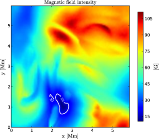
Figure 6.32: Real magnetic field intensity in layers of the model with $\tau_{8542}=1$.

However, the lower-level critical Hanle field given by Eq. (2.36) depends on the mean intensity, and the mean intensity could change significantly with the temperature stratification. In a model atmosphere we can directly get the number of photons per radiation field mode $\mathrm{\bar{n}=J^{0}_{0}(\nu_{0})\cdot c^{2}/(2h\nu^{3}_{0}})$, which give us the lifetime of the level:

$$\frac{1}{t_{\rm life}}\,=\,A_{u{\ell}}\frac{2J_{u}+1}{2J_{\ell}+1}\bar{n}(\tau=1)$$ (6.21)

But usually we can not access the radiation field for making estimations, during an observation for instance. For those cases, let us define a radiation temperature ${\rm T_{rad}}$ that yields a Planck function value $\mathrm{B_{\nu}(T_{rad})}$ equals to the mean intensity $\mathrm{J^{0}_{0}(\nu_{0})}$. Equivalently,

$$\bar{n}\,=\,\frac{1}{e^{\frac{h\nu}{KT_{\rm rad}}}-1}$$ (6.22)

In LTE, $\rm{T_{rad}}$ is the temperature of the plasma but in NLTE it is only a representative number that serves as an upper limit to the local plasma temperature. Then, a change in temperature could produce an effective shift in the magnetic field regime making the polarization to be sensitive to the Hanle effect. For instance, to obtain a critical Hanle field of $5$ G producing a saturation around $50$ G, we would get from Eq.(6.21) a radiation temperature $\mathrm{T_{rad}}\sim 118$ kK for the $8662$ Å line and $\mathrm{T_{rad}}\sim 260$ kK for the $8662$ Å.

We see that larger temperatures are compatible with larger critical fields, what changes the range of validity of the Hanle effect. For this change to occur, the temperature increment has to be in the formation region, where the density of Ca ii is significant. The calculated large temperature values could be possible in the the upper parts of extra hot chromospheric stratifications or inside very hot plasma bubbles (the analyzed models show such anomalous bubbles in a few regions). At least in the latter case, the population of Ca ii is unsignificant because the ions have been abruptly ionized to Ca iii. Other trigger suspicious of being able to bring the Hanle effect into its non-saturated regime is a shock wave. When passing through the chromosphere, it would make the emergent polarization suddenly sensitive to the magnetic field intensity. This kind of sudden Hanle effect could contribute to the small azimuth shifts appearing in the Fig. (6.31), in hot regions with relatively large velocities. Apart from that, a shock wave also means an increment in the density and an approach of those atmospheric layers to behave as a black body (see second row from the top in Figure 5.3). In such case, the radiation temperature values would be more representative of the local plasma.

The estimation of the Hanle critical field in the above discussion should actually consider the transition rates of all the lines connected to the considered atomic level. For the upper level of the $8542$ Å line, we should apply Eq. (2.36) summing the three Einstein emission coefficients $A_{51}$, $A_{52}$ and $A_{53}$, one per transition decaying from level $5$. In that case, we get ${\rm B_{H}=17}$ G (which sets the maximum detectable field strengths around $100$ G).

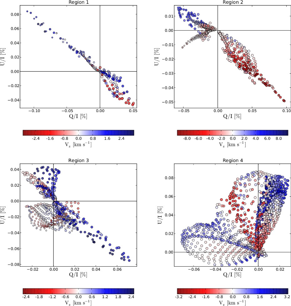
Figure 6.33: Forward scattering Hanle diagrams in the selected regions for the $8662$ Å line. Each small circle is semitransparent and represents a pixel in the corresponding region. The color encodes the value of the vertical velocity and the size of each circle is proportional to the temperature (always at $\tau^{8662}=1$). The upper small panels show the chosen regions (left) and three arbitrary examples (in red) of topological lines (see text).

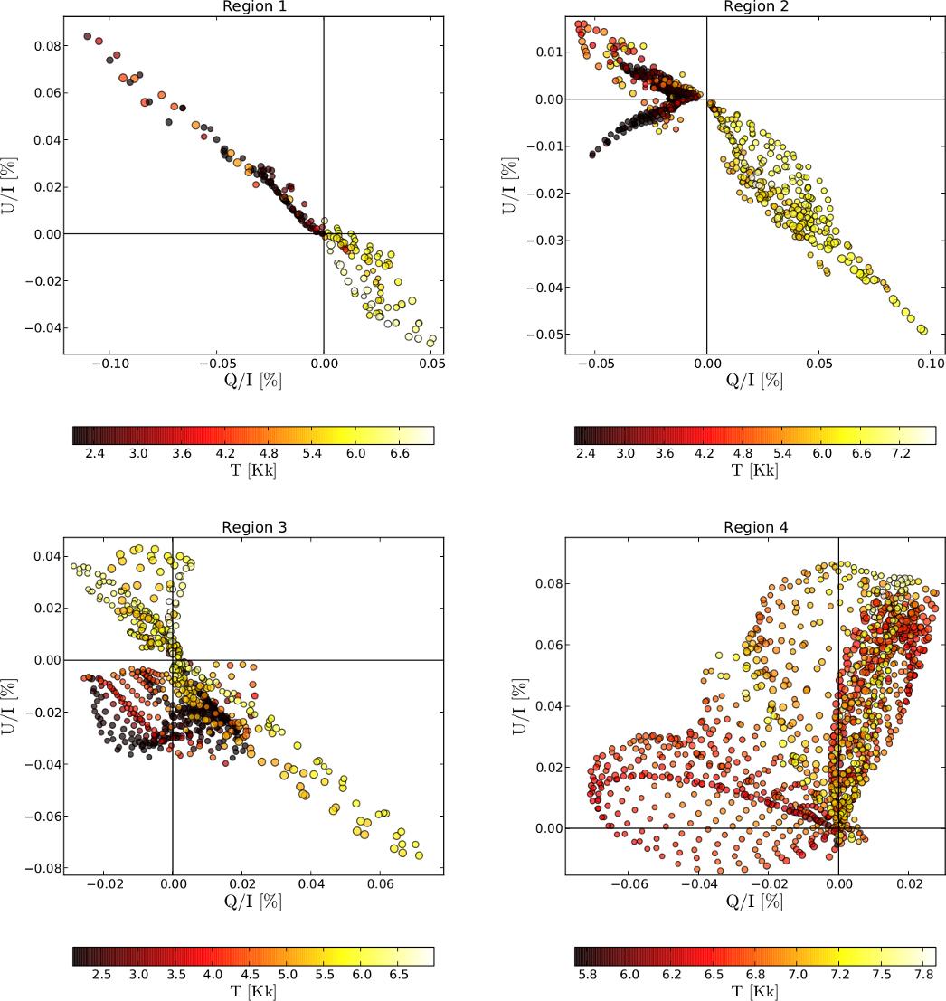
Figure 6.34: Similar to Fig. 6.33, but now the colors encode temperature and the circle size is proportional to the velocity at $\tau^{8662}=1$.

However, it seems to be more precise to estimate the critical field considering only $A_{53}$ ($A_{52}$ is negligible). This way we get $B_{H}=0.82$ G and a better agreement with the Hanle curves calculated by Manso Sainz & Trujillo Bueno (2010) for FALC models, where the upper value for the detectable field strength is $\sim 10$ G.

Hanle diagrams and magnetic field intensity.

More investigation is needed to contrast the previous hypothesis. Meanwhile we can try to deduce something more about the saturation of the Hanle effect through the Hanle diagrams (Figures 6.33, 6.34 above and A.9, A.10 and A.11 in the appendix). By comparing the Hanle diagrams resulting from our calculations in the $8662$ Å line (Figures 6.33 and 6.34) with the corresponding ones of Manso Sainz & Trujillo Bueno (2010) (Figures 14 and 15), we try to know whether this line is really affected by the magnetic field intensity.

First, consider the four regions in the upper panel of Figure 6.33, all of them with considerable magnetic field inclination (HF region); the small Region 1 has an expanding chromosphere with significant velocity; the region 2 has a cool area with patches in different states of motion: static, upward and downward (having a supersonic downflow); the region 3 is composed by a cool compressed bubble and an elongated fringe of pixels with expanding hot atmospheres; finally, the big and hot region 4, not significantly dynamic and with a strong horizontal magnetic field.

We have included information about the vertical velocity and the temperature at $\tau=1$ in the corresponding Hanle diagrams in order to offer an aditional clarifying perspective that can not be achieved observationally (see footnotes in Fig. 6.33 and Fig. 6.34). The colours in the diagram help to identify the different subregions in each region.

After studying these areas and their corresponding Hanle diagrams, we conclude that the Hanle effect is efectively saturated, consistently to what has been assumed in previous sections. To support it, we have shown that the variations in Q and U shown in the Hanle diagrams of Figures 6.33, 6.34 (and similar ones in Appendix) can be understood without any variation of the magnetic field intensity.

Consider that the expressions for $\rm{Q/I}$ and $\rm{U/I}$ appearing in Eqs. (6.4) can be seen as curves in polar coordinates (Eqs. 6.24 a and b), where the radius depends on the inclination of the magnetic field and on the thermodynamic factor $\rm{\mathcal{F}}$:

$$\mathrm{\left(\frac{Q}{I}\right)} =\,r(\mathcal{F},\theta_{B})\cdot\cos{2\chi_{B}},$$ (6.23a)

$$\mathrm{\left(\frac{U}{I}\right)} =\,r(\mathcal{F},\theta_{B})\cdot\sin{2\chi_{B}}.$$ (6.23b)

Assuming first a constant $\rm{\mathcal{F}}$, we stablished simple (linear) ligatures between the azimuth and the inclination of the magnetic field through Eqs. (6.24):

$$2\chi_{B} =\,\rm{2\chi^{i}_{B}+2K\cdot\frac{\chi^{f}_{B}-\chi^{i}_{B}}{\theta^{f}_{B}-\theta^{i}_{B}}\cdot(\theta_{B}-\theta^{i}_{B})},$$ (6.24a)

$$\rm{(\theta^{i}_{B},\theta^{f}_{B})} =\,\rm{(\theta_{V},\pi-\theta_{V})}=\,(54.73\,\mbox{${}^{\circ}$},125.26\,\mbox{${}^{\circ}$}),$$ (6.24b)

where K is a free parameter. The ligature tights the initial and final values of the magnetic field azimuth $\rm{(\chi^{i}_{B},\chi^{f}_{B})}$ with the corresponding initial and final inclination values $\rm{(\theta^{i}_{B},\theta^{f}_{B})}$ of the topologic lines that connect two chosen initial and final points in the spatial maps (see Figs. 6.33 and 6.5). In the following, consider that such points are at both frontiers of the HF regions (in the Van-Vleck HPILs), in such a way that the initial and final values of the magnetic field inclination are given by Eq. (6.24b). Then, choosing different initial and final values for the azimuth in those two points and fixing the number K, we can fit different curves in the Hanle diagrams that correspond to different “topologic” lines crossing the formation region in HF areas of the spatial maps (Fig. 6.35). Then, the magnetic field lines can be inferred from those topologic lines using the magnetic field azimuth in the map. We leave the details for future works.

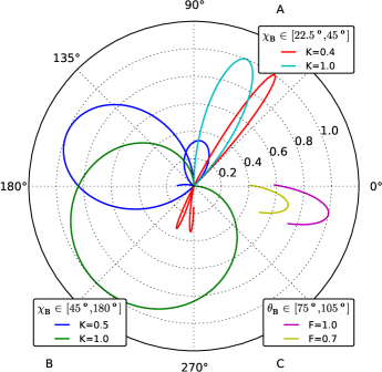
Figure 6.35: Theoretical fit of the Hanle diagrams for three different combinations of parameters (see text and legends).

Note that for a constant azimuth, Q and U only can vary radially. In that case, the topologic lines in the spatial maps would be represented by dots radially aligned in the Hanle diagrams (see Regions $1$ and $2$ showing those radial dependencies). For the dots to describe a loop in the Hanle diagram, it is needed an azimuthal variation along the topologic lines in the spatial maps. The ligature in Eq. (6.24) is thus needed to tie the variation in the azimuth relative to the variation in inclination (or in $\rm{\mathcal{F}}$), and the parametrization is used to adjust such variation to the different cases. The study of the effect of the parameter K seems to be very effective to discard magnetic lines with impossible or improbable topologies. Only a few possibilities give qualitative fits to the Hanle diagram curves. Note that, as we can match the points in the Hanle diagram with the pixels they represent in the spatial maps, we can literally trace the possible magnetic field lines in the HF region. More than that, we can infer the inclination of the field along them. This procedure is facilitated by the knowledge of the location of the main Van-Vleck HPILs because they are placed where the magnetic field topology can be determined with more precision, so acting as boundary conditions.

Some examples of the theoretical curves that explain the loops and bows of the Hanle diagrams can be compared with Fig. 6.35. The narrow bows (e.g., red curve) can be explained with small differences in azimuth between the beginning and the end of a field line. Allowing the action of the thermodinamical variations we can explain the modulation in amplitude of the loops (as shown by the lines in the legend C of Fig. 6.35). In this case, it is specially clear the signature of the strong velocity gradients. When they are present, the polarization is significatively amplified in a small region where the azimuth can not vary at the same rithm, so generating characteristic radial excursions of the points in the Hanle diagrams (Regions 1 and 2 in Fig. 6.33). Choosing larger K values (but below K$=1$), we can explain topologic lines with larger longitudes in the spatial map, corresponded with wider loops in the Hanle diagrams (e.g., blue curves). Finally, the effect of reducing the boundary magnetic field inclinations is a truncation of the loops that result in arcs (again reproduced in the legend- C lines) as the ones appearing in the left upper corner of Region 2 panels in Fig. 6.34 for instance. This latter case is interesting because it would allow us to identify the magnetic field lines that enter in the chromosphere with lower inclinations, which is a marker of lines starting to emerge from the photosphere. There are similar combinations that seems very promising for measuring the topology of the magnetic field, at least in the synthetic maps.

For the moment, we conclude that the Hanle diagrams are a possible solution to observationally distinguish the saturation of the Hanle effect. Furthermore, they can be also a valuable tool for fitting the magnetic field inclinations in chromospheric quiet regions and for studying the precise topology of the magnetic field in observations with good resolution. Results deriving from this ideas will be tackled in future works.

Chapter 7 Conclusions and future work

In this thesis we have carried out a detailed radiative transfer investigation of the linear and circular polarization signals of the Ca ii IR triplet lines produced by scattering processes and the Hanle and Zeeman effects in a variety of dynamical models of the solar chromosphere. The investigation has focussed on the effect that the macroscopic vertical velocity fields and the shock waves of the chromospheric models have on the linear polarization (LP), but taking into account also the combined influence of the thermodynamic and magnetic field topology. The thesis has been complemented with the development of radiative transfer, visualization and analysis tools. Our results will help to confront several chromospheric models of the quiet Sun with real observations through the synthesis of Stokes profiles.

7.1 Goals achieved

The main goals of this thesis have been the following ones:

• We have extended the RT code developed by Manso Sainz & Trujillo Bueno (2003b) to treat a large number of atmosphere models, including the effect of the macroscopic vertical velocity fields on the scattering polarization signals.

• We have shown, quantified and explained the effects that the macroscopic vertical velocity fields can have on the scattering polarization signals, pointing out some unknown diagnostic capabilities of the Ca ii IR triplet lines for studying the solar chromosphere.

• We have calculated temporal series of scattering polarization signals including the effect of the chromospheric velocity fields and temperature shocks on the atomic polarization of the Ca ii levels.

• We have calculated spatial maps of scattering polarization signals including the impact of the atomic level polarization, macroscopic vertical velocities and the Hanle effect in forward scattering geometry.

• We have obtained theoretical LP references for the amplitudes of the $8498$, $8542$ and $8662$ Å lines in dynamic solar model atmospheres. First, in close-to-limb observations, the references are given by the non-magnetic situation. Second, in forward scattering, the reference polarization is given by the maximum amplitudes obtained with a horizontal field in the saturation regime of the Hanle effect. These references can be used to estimate magnetic field strengths using the line-ratio technique.

• We have pointed out a new strategy that can be useful for chromospheric diagnostics (Hanle Polarity Inversion Lines, references for the LP signs, magnetic field inference in forward scattering).

• We have studied the relevance of temperature and macroscopic vertical velocity fields on the calculation of the chromospheric magnetic field orientation, in the presence of the $90\,\mbox{${}^{\circ}$}$ and $180\,\mbox{${}^{\circ}$}$ ambiguities of the Hanle effect.

• We studied the feasibility of using Solar-C and EST to detect the LP features found in our calculations.

• We have calculated a synthetic PCA basis of scattering polarization signals produced in dynamic chomospheric models. Among other things, it can be used to explain real observations in the Ca ii IR triplet lines.

7.2 Conclusions

The main conclusions that have been obtained in this work are:

• When macroscopic vertical velocity gradients are considered in our model atmospheres, the resulting polarization profiles of the Ca ii IR triplet lines are asymmetrized, shifted in wavelength, and modulated in amplitude with respect to the constant velocity case. We remark that these effects depend on the velocity gradient. Thus, larger velocities do not mean larger variations in the LP if no significant velocity gradient is located in the line formation region.

• The fundamental mechanism explaining the LP signals under dynamic circumstances is that increments in the absolute value of the velocity gradient increase the source function (Doppler brightening) and enhance the anisotropy of the radiation field at some heights. The result is a subsequent enhancement of the atomic alignment of the upper and lower levels controling the linear polarization profiles of the line transition under consideration (Doppler-induced modulation).

• A second mechanism explains why sometimes the variations in the anisotropy produce an amplification of the LP signals and why sometimes they produce a reduced amplitude or a sign reversal. The emergent LP is the result of the atomic alignment values of the lower and upper levels of the line transition at every height in the formation region. The variation with height of such atomic aligments is such that they are equal at a given chromospheric layer in the formation region. The atomic alignment of one of the line levels dominates the LP above such intersection layer, while the one of the other level dominates below. Then, the relative location of the levels’s alignment intersection with respect to the heights where the anisotropy has been enhanced makes the alignment of one of the line levels to be preferentially increased. The details of this situation alter the shapes, amplitudes and signs of the LP profiles.

• The shapes, signs and amplitudes of the LP signals of the IR triplet lines change significantly with the line of sight, because the height of formation moves with respect to the alignment intersection height.

• In general, the modulation of the LP signals produced by macroscopic vertical velocity fields does not have the same importance for all atomic transitions. Strong spectral lines with wide absorption profiles (e.g., with large thermal widths) require larger vertical velocities than weaker spectral lines in order to experiment the same amplitude variation in their scattering polarization signals. Some spectral lines (e.g., the Ca ii IR triplet) forming in chromospheric layers (where the velocity gradients are significant) and whose atomic levels can be polarized are expected to be sensitive to Doppler-induced modulations in their LP profiles.

• The quantitative variations of the LP signals produced by velocity gradients depend on the strength of the model dynamics. In highly dynamic chromospheric models, the variations of the LP in close-to-limb observations give clear patterns characteristic of the presence of shocks in the models.

• The close-to-limb synthesis carried out in the considered 1D time-dependent models show that the velocity gradients produce a significant size variation of the scattering polarization signals. In this case, the maximum enhancement factors of the emergent linear polarization are $\sim 10$ (in the $8498$ Å line) and $\sim 7$ (in the $8542$ Å and $8662$ Å lines), for the instantaneous values of the $\rm{Q/I}$ amplitudes with respect to the static FAL-C case. If we consider temporal averages of the emergent Stokes profiles during periods of several minutes, we get amplification factors of about a factor of two (time-averaged Q/I amplitudes reach $\sim 1\,\%$) in the $8542$ Å and $8662$ Å lines, and a sign reversal with antisymmetric profiles in the LP signals of the $8498$ Å line. The lack of spatial or temporal coherence and resolution in the low-chromosphere dynamics could make the $\lambda 8498$ signals to cancel out due to its variable polarity.

• The velocity-free approximation is not valid to calculate the emergent scattering polarization signals in the presence of velocity gradients because it does not capture the effect of the dynamics on the atomic level polarization. Such approximation gives polarization amplitudes that are not enhanced with respect to the static case.

• The forward scattering RT calculations carried out in the considered MHD models (Leenaarts et al., 2009a) show a sparse spatial distribution of pixels with amplitudes significantly larger than in the static case. On the one hand, the reason is that the considered MHD model is significantly less dynamic than the 1D dynamical models we have analyzed. On the other hand, the variations in the radiation field anisotropy induced by the temperature gradients of the MHD model result in LP amplitudes that are often significantly larger than in the semi-empirical model considered by Manso Sainz & Trujillo Bueno (2010).

• In principle, the inference of chromospheric magnetic fields with the Hanle effect can be affected by the dynamic state of the atmosphere because the LP amplitudes of the Ca ii lines are modulated by the vertical velocities. In order to give a precise magnetic field estimation of the quiet solar chromosphere it is then necessary to consider the polarization amplitude variations sourced by the dynamics of the chromosphere. However, we expect this effect to be small in low-resolution chromospheric observations.

• We propose the so-called Hanle Polarity Inversion Lines (HPILs) as features that can help to deduce the magnetic field vector in quiet Sun chromospheric maps of the LP signals in IR Ca ii lines. They give useful references to constrain the orientation of the magnetic field as well as its variation with height (when analyzed simultaneously in more than one spectral line).

• The thermodynamic HPILs are sensitive to very specific stratifications of the radiation field anisotropy; they allowed us to find the location of cool chromospheric bubbles of plasma using the LP signals.

• The Van-Vleck HPILs in the Ca ii IR triplet lines give the locations where the chromospheric magnetic field has an inclination of $54.73\,\mbox{${}^{\circ}$}$ or $125.27\,\mbox{${}^{\circ}$}$.

• The behavior of the scattering polarization signals in the weak field regime makes the stratification of temperature, velocity and magnetic inclination to influence the inference of the magnetic field azimuth from Stokes Q and U. To illustrate and quantify these dependencies we have simulated the process of magnetic field inference from spatial maps of the Stokes vector. This study could be considered as an extension to the work of Manso Sainz & Trujillo Bueno (2010) in more realistic atmospheric models.

• Studying the scattering polarization signals under dynamic situations, we have given a table of signs of reference for the LP signals of the Ca ii IR triplet lines in the most important physical circumstances describing the considered MHD models. These references can be used to break the $90\,\mbox{${}^{\circ}$}$ magnetic field ambiguity existing in the weak field regime. They can also be used to diagnose the basic physical state of the chromosphere in pixels showing those LP signs. The LP signs are compatible with the results of Manso Sainz & Trujillo Bueno (2010).

• The dependence of the analyzed scattering polarization signals on temperature, velocity and magnetic field stratification has allowed the identification of some simple diagnostic techniques based on the signs of the LP profiles of the Ca ii IR triplet under different physical situations.

• Our calculations show that the real relevance of the chromospheric vertical velocity fields is missed with the current instrumental sensitivities and telescope apertures. This explain that we cannot observe such effects until more powerful instrumentation is developed.

• Our calculations point out that the Solar-C telescope and perhaps the European Solar Telescope should be able to capture the behavior of the scattering polarization signals that we have described in this thesis for the IR triplet of the Ca ii. The best strategy to improve the signal-to-noise ratio of such measurements without losing spatial and temporal resolution is a combination of short temporal integrations and PCA postprocessing.

7.3 Future work

The MHD models of the solar atmosphere are evolving more quickly than the radiative transfer codes with capabilities to treat the scattering polarization. Thus, despite the fact that the synthesis of Stokes profiles is limited by the realism of MHD models, the very first technical limitation is the intrinsic difficulty of the detailed RT problem with polarization: its highly non-linear and non-local nature, the demanding spatial and angular resolution that it requires and the involved physics to solve it. A giant leap is required in the way we solve these problems. I plan to continue the research on new methods that allow a faster resolution of three dimensional radiative transfer problems. This will allow a natural extension of this thesis to treat the more general problem in which the horizontal macroscopic flows are included.

Using state-of-the-art MHD models, I would like to continue exploring the spectropolarimetric characterization of chromospheric solar structures. This alternative seeks to identify spatiotemporal polarization patterns (in synthetic or real profiles), such as those identified in Chapters 5 and 6 (e.g., shocks fingerprints in temporal series and Hanle PILs in spatial maps).

An important step after this thesis will be however to carry out spectropolarimetric observations and to try to interpret them applying the results of this work. It would be of great interest to detect LP features confirming our results in the solar chromosphere as well as to apply the proposed diagnosis methods to real observations. However, the current instrumentation does not have enough sensitivity to capture the dynamic effects on the scattering polarization. In the future, with the arrival of the new solar facilities, such as SOLAR-C, ATST or EST, a new world of possibilities will be opened.

Meanwhile, we could try to validate our results in stronger spectral lines whose scattering polarization could also be affected by shocks and motions (e.g., the Na i D lines or the Ca i $4227$ Å line). In particular, the Cai $4227$ Å line can be a good candidate to follow up the ideas of Chapter 6, which explored the forward scattering geometry as a way of inferring information about solar magnetic fields in situations where the linear polarization is dominated by scattering and Hanle processes.

Other issue to solve is the inference of the magnetic field azimuth in the presence of significant velocity fields or temperature gradients, which produce a lack of precision in such estimation (at least in our theoretical results). How can our results be extrapolated to chromospheres with stronger magnetic fields?Are the linear polarization signals similarly modified by thermodynamic gradients in such cases?

Appendix A Appendix.

A.1 Special functions in section 4.3.1

Introducing Equation 4.10 into Equation 4.2.1

$$\begin{split}\bar{J}^{0}_{0}=&\frac{1}{2}\int_{0}^{\infty}d\nu^{\prime}\frac{1}{\sqrt{\pi}\Delta\nu_{D}}\exp\{-(\frac{\nu^{\prime}-\nu_{0}}{\Delta\nu_{D}})^{2}\}\\ &\int_{0}^{1}d\mu I^{(0)}(1-u+u\mu)[1-a\exp\{-(\frac{\nu^{\prime}(1+v_{z}\mu/c)-\nu_{0}}{w})^{2}\}].\end{split}$$ (A.1)

Introducing the variables $x=(\nu^{\prime}-\nu_{0})/w$, $\alpha=\Delta\nu_{D}/w$, and $\xi=v_{z}\nu_{0}/(cw)$, then the mean intensity in the comoving frame

$$\frac{\bar{J}^{0}_{0}}{I^{(0)}}=\frac{1}{2}\int_{-\infty}^{\infty}dx\frac{1}{\sqrt{\pi}\alpha}{e}^{-(x/\alpha)^{2}}\int_{0}^{1}d\mu(1-u+u\mu)(1-ae^{-(x+\xi\mu)^{2}}).$$ (A.2)

In passing from Equation (A.1) to Equation (A.2), we have extended the integration limit on $x$ to $\infty$. Analogously for the anisotropy in the comoving frame

$$\frac{\bar{J}^{2}_{0}}{I^{(0)}}=\frac{1}{4\sqrt{2}}\int_{-\infty}^{\infty}dx\frac{1}{\sqrt{\pi}\alpha}{\rm e}^{-(x/\alpha)^{2}}\int_{0}^{1}d\mu(3\mu^{2}-1)(1-u+u\mu)(1-a{\rm e}^{-(x+\xi\mu)^{2}}).$$ (A.3)

The following integrals are easily evaluated (see Spiegel, 1998)

$${\cal I}_{0}(\alpha;\xi) \equiv\int_{-\infty}^{\infty}dx\frac{1}{\sqrt{\pi}\alpha}{\rm e}^{-(x/\alpha)^{2}}\int_{0}^{1}(1-u+u\mu)[1-a{\rm e}^{-(x+\xi\mu)^{2}}]d\mu$$

$$=\frac{1}{2}[2-u+a(u-1)\sqrt{\pi}\frac{1}{\xi}{\rm Erf}(\frac{\xi}{\sqrt{1+\alpha^{2}}})+au\sqrt{1+\alpha^{2}}\frac{1}{\xi^{2}}(\exp\{-\frac{\xi^{2}}{1+\alpha^{2}}\}-1)],$$ (A.4)

$${\cal I}_{2}(\alpha;\xi) \equiv\int_{-\infty}^{\infty}dx\frac{1}{\sqrt{\pi}\alpha}{\rm e}^{-(x/\alpha)^{2}}\int_{0}^{1}(3\mu^{2}-1)(1-u-u\mu)[1-a{\rm e}^{-(x+\xi\mu)^{2}}]d\mu$$

$$=\frac{1}{4}[u-2a(u-1)\sqrt{\pi}\frac{1}{\xi}{\rm Erf}(\frac{\xi}{\sqrt{1+\alpha^{2}}})+2a\sqrt{1+\alpha^{2}}\frac{1}{\xi^{2}}\left[u+(3-u)\exp\{-\frac{\xi^{2}}{1+\alpha^{2}}\}\right]$$ (A.5)

$$+3a(u-1)(1+\alpha^{2})\sqrt{\pi}\frac{1}{\xi^{3}}{\rm Erf}(\frac{\xi}{\sqrt{1+\alpha^{2}}})+6au(1+\alpha^{2})^{3/2}\frac{1}{\xi^{4}}(\exp\{-\frac{\xi^{2}}{1+\alpha^{2}}\}-1)],$$

where we have made use of

$$\int_{-\infty}^{\infty}dx\frac{1}{\sqrt{\pi}\alpha}{\rm e}^{-(x/\alpha)^{2}}[1-a{\rm e}^{-(x+\xi\mu)^{2}}]=1-\frac{a}{\sqrt{1+\alpha^{2}}}\exp\{-\frac{\mu^{2}\xi^{2}}{1+\alpha^{2}}\}.$$ (A.6)

From them, the values for $\bar{J}^{0}_{0}$ and the anisotropy $\sqrt{2}\bar{J}^{2}_{0}/\bar{J}^{0}_{0}$ are trivially derived.

In the high velocity limit ($\xi\rightarrow\infty$), ${\cal I}_{0}(\alpha;\xi)=(2-u)/2$, and ${\cal I}_{2}(\alpha;\xi)=u/4$ (regardless of $\alpha$). In the low velocity limit:

$${\cal I}_{0}(\alpha;\xi) =\frac{1}{2}(1-\frac{a}{\sqrt{1+\alpha^{2}}})(2-u)+\frac{a(4-u)}{12(1+\alpha^{2})^{3/2}}\xi^{2}+{\rm O}(\xi^{3}),$$ (A.7)

$${\cal I}_{2}(\alpha;\xi) =\frac{u}{4}(1-\frac{a}{\sqrt{1+\alpha^{2}}})+\frac{a(16-u)}{60(1+\alpha^{2})^{3/2}}\xi^{2}+{\rm O}(\xi^{3}).$$ (A.8)

A.2 Statistical equilibrium equations in the non-magnetic case.

The rate equations for the considered problem are as follow. They have been obtained by particularizing to the model-atom of Fig.1 the equations contained in Sects. 7.2 and 7.13 of Landi Degl’Innocenti & Landolfi (2004).

$$\begin{split}\frac{\rm d}{{\rm d}t}\rho^{0}_{0}(1)=&-\biggl{[}\sum_{u=4}^{5}B_{1u}\bar{J}^{0}_{0}(1\rightarrow u)+\sum_{i\neq 1}C_{1i}\biggr{]}\rho^{0}_{0}(1)+A_{41}\rho^{0}_{0}(4)\\ &+\sqrt{2}A_{51}\rho^{0}_{0}(5)+\sum_{i\neq 1}C_{i1}\sqrt{\frac{2J_{i}+1}{2}}\rho^{0}_{0}(i),\end{split}$$ (A.9)

$$\begin{split}\frac{\rm d}{{\rm d}t}\rho^{0}_{0}(2)=&-\biggl{[}\sum_{u=4}^{5}B_{2u}\bar{J}^{0}_{0}(2\rightarrow u)+\sum_{i\neq 2}C_{2i}\biggr{]}\rho^{0}_{0}(2)-\biggl{(}\frac{1}{\sqrt{2}}B_{24}\bar{J}^{2}_{0}(2\rightarrow 4)-\frac{2\sqrt{2}}{5}B_{25}\bar{J}^{2}_{0}(2\rightarrow 5)\biggr{)}\rho^{2}_{0}(2)\\ &+\frac{1}{\sqrt{2}}A_{42}\rho^{0}_{0}(4)+A_{52}\rho^{0}_{0}(5)+\sum_{i\neq 2}C_{i2}\frac{\sqrt{2J_{i}+1}}{2}\rho^{0}_{0}(i),\end{split}$$ (A.10)

$$\begin{split}\frac{\rm d}{{\rm d}t}\rho^{0}_{0}(3)=&-\biggl{[}B_{35}\bar{J}^{0}_{0}(3\rightarrow 5)+\sum_{i\neq 3}C_{3i}\biggr{]}\rho^{0}_{0}(3)-\frac{\sqrt{7}}{5}B_{35}\bar{J}^{2}_{0}(3\rightarrow 5)\rho^{2}_{0}(3)\\ &+\sqrt{\frac{2}{3}}A_{53}\rho^{0}_{0}(5)+\sum_{i\neq 3}C_{i3}\sqrt{\frac{2J_{i}+1}{6}}\rho^{0}_{0}(i),\end{split}$$ (A.11)

$$\begin{split}\frac{\rm d}{{\rm d}t}\rho^{0}_{0}(4)=&-\biggl{[}\sum_{l=1}^{2}A_{4l}+\sum_{i\neq 4}C_{4i}\biggr{]}\rho^{0}_{0}(4)+\sum_{l=1}^{2}B_{l4}\bar{J}^{0}_{0}(l\rightarrow 4)\sqrt{\frac{2J_{l}+1}{2}}\rho^{0}_{0}(l)\\ &+B_{24}\bar{J}^{2}_{0}(l\rightarrow 4)\rho^{2}_{0}(2)+\sum_{i\neq 4}C_{i4}\sqrt{\frac{2J_{i}+1}{2}}\rho^{0}_{0}(i),\end{split}$$ (A.12)

$$\linebreak\begin{split}\frac{\rm d}{{\rm d}t}\rho^{0}_{0}(5)=&-\biggl{[}\sum_{l=1}^{3}A_{5l}+\sum_{i\neq 5}C_{5i}\biggr{]}\rho^{0}_{0}(5)+\sum_{l=1}^{3}B_{l5}\bar{J}^{0}_{0}(l\rightarrow 5)\frac{\sqrt{2J_{l}+1}}{2}\rho^{0}_{0}(l)\\ &-\frac{2\sqrt{2}}{5}B_{25}\bar{J}^{2}_{0}(2\rightarrow 5)\rho^{2}_{0}(2)+\frac{\sqrt{42}}{10}B_{35}\bar{J}^{2}_{0}(3\rightarrow 5)\rho^{2}_{0}(3)+\sum_{i\neq 5}C_{i5}\frac{\sqrt{2J_{i}+1}}{2}\rho^{0}_{0}(i),\end{split}$$ (A.13)

$$\begin{split}\frac{\rm d}{{\rm d}t}\rho^{2}_{0}(2)=&-\biggl{[}\sum_{u=4}^{5}B_{2u}\bar{J}^{0}_{0}(2\rightarrow u)+\sum_{i\neq 2}C_{2i}+D_{2}^{(2)}\biggr{]}\rho^{2}_{0}(2)-\biggl{(}\frac{1}{\sqrt{2}}B_{24}\bar{J}^{2}_{0}(2\rightarrow 4)\\ &-\frac{2\sqrt{2}}{5}B_{25}\bar{J}^{2}_{0}(2\rightarrow 5)\biggr{)}\rho^{0}_{0}(2)+\frac{1}{5}A_{52}\rho^{2}_{0}(5)+\sum_{i=3,5}C_{i2}^{(2)}\frac{\sqrt{2J_{i}+1}}{2}\rho^{2}_{0}(i),\end{split}$$ (A.14)

$$\begin{split}\frac{\rm d}{{\rm d}t}\rho^{2}_{0}(3)=&-\biggl{[}B_{35}\bar{J}^{0}_{0}(3\rightarrow 5)+\sum_{i\neq 3}C_{3i}+D_{3}^{(2)}\biggr{]}\rho^{2}_{0}(3)-B_{35}\bar{J}^{2}_{0}(3\rightarrow 5)\frac{\sqrt{7}}{5}\rho^{0}_{0}(3)\\ &+B_{35}\bar{J}^{2}_{0}(3\rightarrow 5)\biggl{[}\sqrt{\frac{5}{7}}\rho^{2}_{0}(3)-\frac{9}{2}\sqrt{\frac{3}{35}}\rho^{4}_{0}(3)\biggr{]}+\frac{2}{5}\sqrt{\frac{7}{3}}A_{53}\rho^{2}_{0}(5)\\ &+\sum_{i=2,5}C_{i3}^{(2)}\sqrt{\frac{2J_{i}+1}{6}}\rho^{2}_{0}(i),\end{split}$$ (A.15)

$$\begin{split}\frac{\rm d}{{\rm d}t}\rho^{2}_{0}(5)=&-\biggl{[}\sum_{l=1}^{3}A_{5l}+\sum_{i\neq 5}C_{5i}+D_{5}^{(2)}\biggr{]}\rho^{2}_{0}(5)+\frac{1}{5}B_{25}\bar{J}^{0}_{0}(2\rightarrow 5)\rho^{2}_{0}(2)\\ &+\frac{\sqrt{21}}{5}B_{35}\bar{J}^{0}_{0}(3\rightarrow 5)\rho^{2}_{0}(3)+\frac{1}{2}B_{15}\bar{J}^{2}_{0}(1\rightarrow 5)\rho^{0}_{0}(1)-\frac{2\sqrt{2}}{5}B_{25}\bar{J}^{2}_{0}(2\rightarrow 5)\rho^{0}_{0}(2)\\ &+\frac{\sqrt{3}}{10}B_{35}\bar{J}^{2}_{0}(3\rightarrow 5)\rho^{0}_{0}(3)+2\sqrt{\frac{7}{5}}B_{25}\bar{J}^{2}_{0}(2\rightarrow 5)\rho^{2}_{0}(2)-\sqrt{\frac{3}{5}}B_{35}\bar{J}^{2}_{0}(3\rightarrow 5)\rho^{2}_{0}(3)\\ &+\frac{9}{\sqrt{5}}B_{35}\bar{J}^{2}_{0}(3\rightarrow 5)\rho^{4}_{0}(3)+\sum_{i=2,3}C_{i5}^{(2)}\frac{\sqrt{2J_{i}+1}}{2}\rho^{2}_{0}(i),\end{split}$$ (A.16)

$$\begin{split}\frac{\rm d}{{\rm d}t}\rho^{4}_{0}(3)=&-\biggl{[}B_{35}\bar{J}^{0}_{0}(3\rightarrow 5)+\sum_{i\neq 3}C_{3i}+D_{3}^{(4)}\biggr{]}\rho^{4}_{0}(3)\\ &-B_{35}\bar{J}^{2}_{0}(3\rightarrow 5)\biggl{[}\frac{9}{2}\sqrt{\frac{3}{35}}\rho^{2}_{0}(3)+3\sqrt{\frac{11}{70}}\rho^{4}_{0}(3)\biggr{]},\end{split}$$ (A.17)

where $A_{u{\ell}}$ and $B_{{\ell}u}$ are the Einstein emission and absortion coefficients; $C_{{\ell}u}$ and $C_{u{\ell}}$ are the excitation and deexcitation inelastic collisional rates, respectively; $C^{(2)}_{{\ell}u}$ and $C^{(2)}_{u{\ell}}$ are the collisional transfer rates for alignment between polarizable levels (with $J>1/2$); and $D^{(K)}_{i}$ is the depolarization rate of the $K$-th multipole of level ${i}$ due to elastic collisions with neutral hydrogen atoms. The $\rho^{K}_{0}$ elements are referred to a coordinate system with the quantization axis along the solar local vertical direction.

A.3 Derivation of the fractional linear polarization under EB approximation.

We consider a non-magnetic, static, axisymmetric and semi-infinite atmosphere. With axisymmetric we mean an atmosphere without inhomogeneities around its radial axis. Under this assumptions, symmetry breaking effects are negligible, what in turn nullifies quantum coherences ($\rho^{K}_{Q\neq 0}=0$). Thus, only $\rho^{2}_{0}$ and $\rho^{0}_{0}$ are non-zero, what implies as well that only I and Q are non-zero in the Stokes vector. Then, Eqs. (6) of Sec. 4.2.2 are still valid. They are used in the next demonstration with the only difference that absortion profiles are not affected by dopplershits ($\phi^{\prime}_{lu}=\phi_{lu}$).
The solar atmosphere is weakly anisotropic, so $I\gg Q$. Then, neglecting second order terms in Eqs. (5) of Paper i , and recalling that optical depth seen by a photon along the ray path s is

$$\tau^{\rm los}_{\nu}=-\int\eta_{I}ds,$$

we have the next RTE ’s:

$$\frac{\rm dI}{{\rm d}\tau^{\rm los}} =I-S_{I},$$ (A.18a)

$$\frac{\rm dQ}{{\rm d}\tau^{\rm los}} =Q-S_{Q}.$$ (A.18b)

Source functions for intensity and Stokes Q are $S_{I}=\frac{\epsilon_{I}}{\eta_{I}}$ and $S_{Q}=\frac{\epsilon_{Q}-\eta_{Q}I}{\eta_{I}}$. Under EB approximation the source function $S_{I}$ is developed in power series through optical depth and truncated to first order as $S_{I}(\tau_{\nu})=a+b\tau_{\nu}$ (being a and b arbitrary constants). Thus, taking into account that $\tau_{\nu}=\tau^{\rm los}_{\nu}\cdot\mu$, the solution to the RTE for the emergent intensity is:

$$I_{\nu}(\tau_{\nu},\mu)=a+b(\mu\tau^{\rm los}_{\nu}+\mu).$$ (A.19)

We see that $I_{\nu}(\tau_{\nu}=0)=S_{I}(\tau_{\nu}=\mu)$ or, equivalently, $I_{\nu}(\tau_{\nu}=0)=S_{I}(\tau^{\rm los}_{\nu}=1)$. And from Eq. (A.19) we also note that:

$$\frac{\rm dI}{{\rm d}\tau^{\rm los}}=\frac{\rm dS_{I}}{{\rm d}\tau^{\rm los}}=b\mu.$$

Hereafter, we follow the notation $x^{[r]}$, indicating that the quantity $x$ have to be evaluated at $\tau^{\rm los}_{\nu}=r$. Thus, we can write $b\mu=S^{[1]}_{I}-S^{[0]}_{I}$. Repeating the same considerations, we assume EB as well for Stokes Q and write:

$$S_{Q}(\tau_{\nu})=a^{\prime}+b^{\prime}\tau_{\nu}$$

$$Q_{\nu}(\tau_{\nu},\mu)=a^{\prime}+b^{\prime}(\tau_{\nu}+\mu),$$

$$Q^{[0]}_{\nu}=S^{[1]}_{Q},$$ (A.20)

$$\frac{\rm dQ}{{\rm d}\tau^{\rm los}}=\frac{\rm dS_{Q}}{{\rm d}\tau^{\rm los}}=b^{\prime}\mu=S^{[1]}_{Q}-S^{[0]}_{Q}.$$

With this expressions we can put the emerging relative linear polarization as :

$$\frac{Q^{[0]}}{I^{[0]}}=\frac{S_{Q}^{[1]}}{S_{I}^{[1]}}=\left[\frac{(\epsilon_{Q}-\eta_{Q}I)/\eta_{I}}{\epsilon_{I}/\eta_{I}}\right]^{[1]}=\frac{\epsilon^{[1]}_{Q}}{\epsilon^{[1]}_{I}}-\frac{\eta^{[1]}_{Q}}{\epsilon^{[1]}_{I}}I^{[1]}.$$

The evaluation of $I^{[1]}$ can be done using the RTE or simply realizing that:

$$I^{[1]}=I_{\nu}(\tau^{\rm los}_{\nu}=1)=S^{[2]}_{I}=\frac{\epsilon^{[2]}_{I}}{\eta^{[2]}_{I}},$$

leading to

$$\frac{Q}{I}=\frac{\epsilon^{[1]}_{Q}}{\epsilon^{[1]}_{I}}-\frac{\eta^{[1]}_{Q}\epsilon^{[2]}_{I}}{\eta^{[2]}_{I}\epsilon^{[1]}_{I}}.$$ (A.21)

Until now, we have only imposed axisymmetry and EB. If we also particularize for strong lines ($\epsilon_{I}\approx\epsilon^{\rm line}_{I}$ and $\eta_{I}\approx\eta^{\rm line}_{I}$) and use Eqs. (4.6) of Sec. 4.2.2 for substituting absortion and emission terms, we arrive to:

$$\frac{Q}{I}\approx\frac{3}{2\sqrt{2}}(1-\mu^{2})\left[\omega^{(2)}_{J_{u}J_{l}}\cdot\sigma^{2}_{0}(J_{u})^{[1]}-\omega^{(2)}_{J_{l}J_{u}}\cdot\frac{\rho^{2}_{0}(J_{l})^{[1]}}{\rho^{0}_{0}(J_{u})^{[1]}}\cdot\frac{\rho^{0}_{0}(J_{u})^{[2]}}{\rho^{0}_{0}(J_{l})^{[2]}}\right],$$

Note that the superindex $[2]$ is a notation for optical depth and the superindex $(2)$ has to do with the designation of the quantum numbers decribed in Table 4.1. Multiplying and dividing by $\rho^{0}_{0}(J_{l})^{[1]}$ the expression read

$$\frac{Q}{I}=\frac{3}{2\sqrt{2}}(1-\mu^{2})\left[\omega^{(2)}_{J_{u}J_{l}}\cdot\sigma^{2}_{0}(J_{u})^{[1]}-\omega^{(2)}_{J_{l}J_{u}}\cdot\sigma^{2}_{0}(J_{l})^{[1]}\cdot\textit{A}\right],$$ (A.22)

where the quantity A affecting to the lower level alignment is

$$\textit{A}=\left(\frac{\rho^{0}_{0}(J_{l})}{\rho^{0}_{0}(J_{u})}\right)^{[1]}\cdot\left(\frac{\rho^{0}_{0}(J_{u})}{\rho^{0}_{0}(J_{l})}\right)^{[2]}.$$ (A.23)

If radiative processes dominate over inelastic collisional ones, $\rho^{0}_{0}(J_{u})/\rho^{0}_{0}(J_{l})\approx B_{lu}\cdot\bar{J}^{0}_{0}/A_{ul}$ with very good approximation, and then:

$$\textit{A}\approx\frac{\bar{J}^{0[2]}_{0}}{\bar{J}^{0[1]}_{0}}\ \ \ \ ,$$

It implies that

$$\frac{Q}{I}\approx\frac{3}{2\sqrt{2}}(1-\mu^{2})\left(\omega^{(2)}_{J_{u}J_{l}}\cdot\sigma^{2}_{0}(J_{u})^{[1]}-\omega^{(2)}_{J_{l}J_{u}}\cdot\sigma^{2}_{0}(J_{l})^{[1]}\cdot\frac{\bar{J}^{0[2]}_{0}}{\bar{J}^{0[1]}_{0}}\right)$$ (A.24)

is valid at line center $\lambda_{0}$. The only difference with the equation estimated by Trujillo Bueno (1999) is the factor A, that can be neglected in majority of cases due to its closeness to one. The factor A can be understood as a measure of the mean intensity gradient around $\tau^{\rm los}_{\nu_{0}}=1$, being larger in presence of shocks and heatings. If the gradient of temperature is then significant in that region we could expect this factor to modify the lower level fractional alignment and the estimation of the line center Q/I. Although the proximity of this idea with the main topic of the this thesis, we have not found a clear application to Eq. A.24. We always fix ${\rm A=1}$ and use that equation for explicative purposes in the text.

A.4 Other figures in Chapter 6.

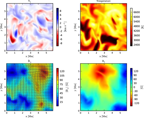
Figure A.1: Physical quantities at $\tau=1$ for the $8498\,$ Å line. Upper left: vertical velocity. Upper right: temperature distribution. Lower left: horizontal magnetic field intensity. Lower right: longitudinal magnetic field intensity.

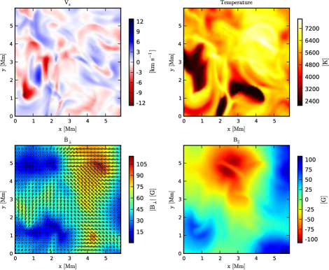
Figure A.2: The same as in Fig. A.1 but for the $8662$ Å line.

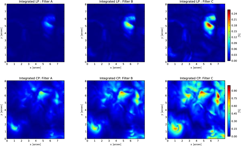
Figure A.3: The same as in Fig. 6.14 but for tke K line.

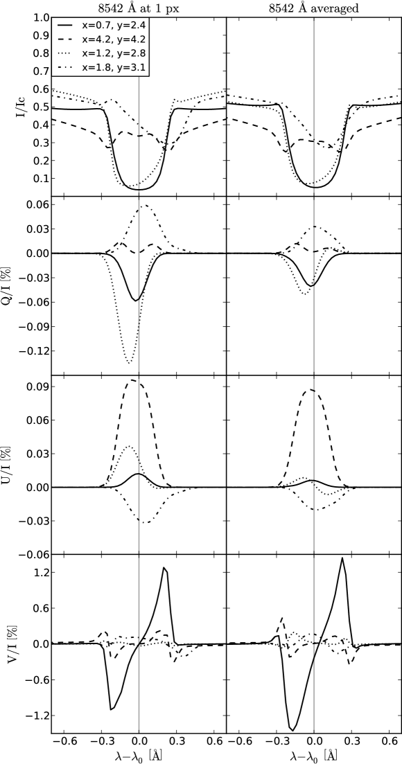
Figure A.4: Effect of averaging across $1$ square arcsecond centered in different pixels (different color identifies different center pixels). The average is done in each Stokes vector component before calculating the fractional quantities.

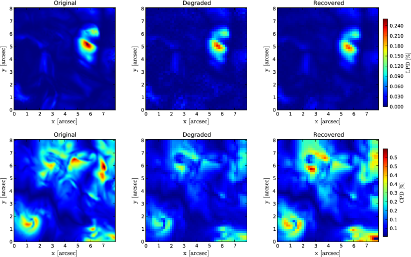
Figure A.5: The same as figure 6.22 but for the K line.

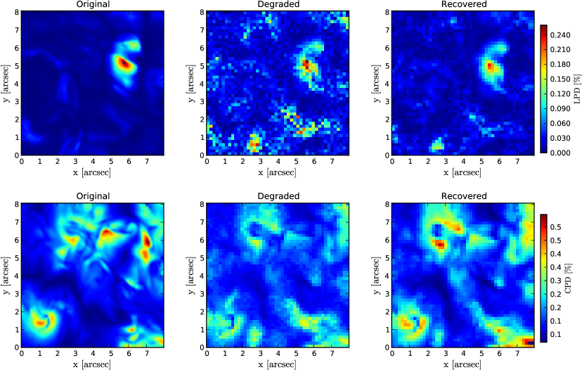
Figure A.6: The same as figure A.5 but with S/N$=10^{-3}$.

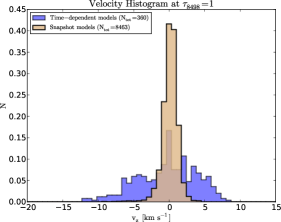
Figure A.7: The same as the left panel of Fig. 6.4 but for the $8498$ Å line.

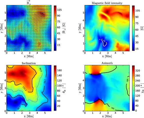
Figure A.8: Detailed description of the magnetic field in $\tau^{8542}=1$. Upper left panel: transversal component of the magnetic. Upper right panel: Intensity of the magnetic field. The white line encloses the area with less than $20$ G. Lower left panel: Inclination of the magnetic field. Solid iso-contours correspond to $\theta_{B}=\theta_{V}$ and $\theta_{B}=\pi-\theta_{V}$ (with $\theta_{V}$ the Van Vleck angle). Lower right panel: Azimut of the magnetic field and iso-contours of $\chi_{B}=180\,\mbox{${}^{\circ}$}$.

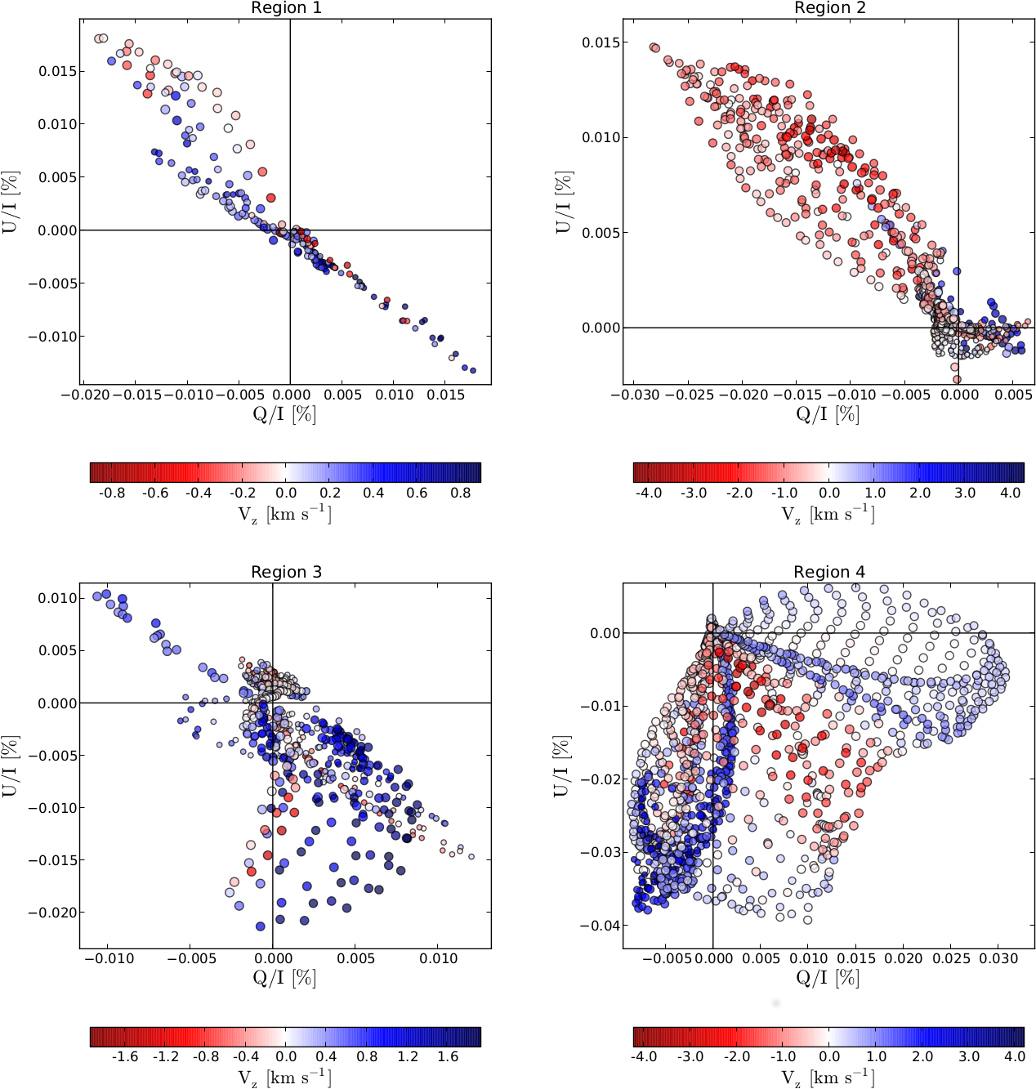
Figure A.9: The same as in Fig. 6.33, but in $8498$ Å.

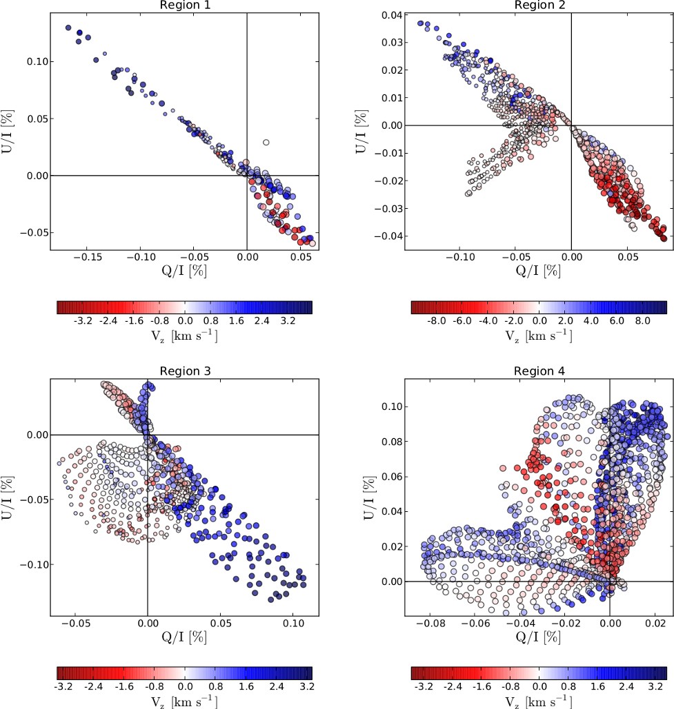
Figure A.10: The same as in Fig. 6.33, but in $8542$ Å.

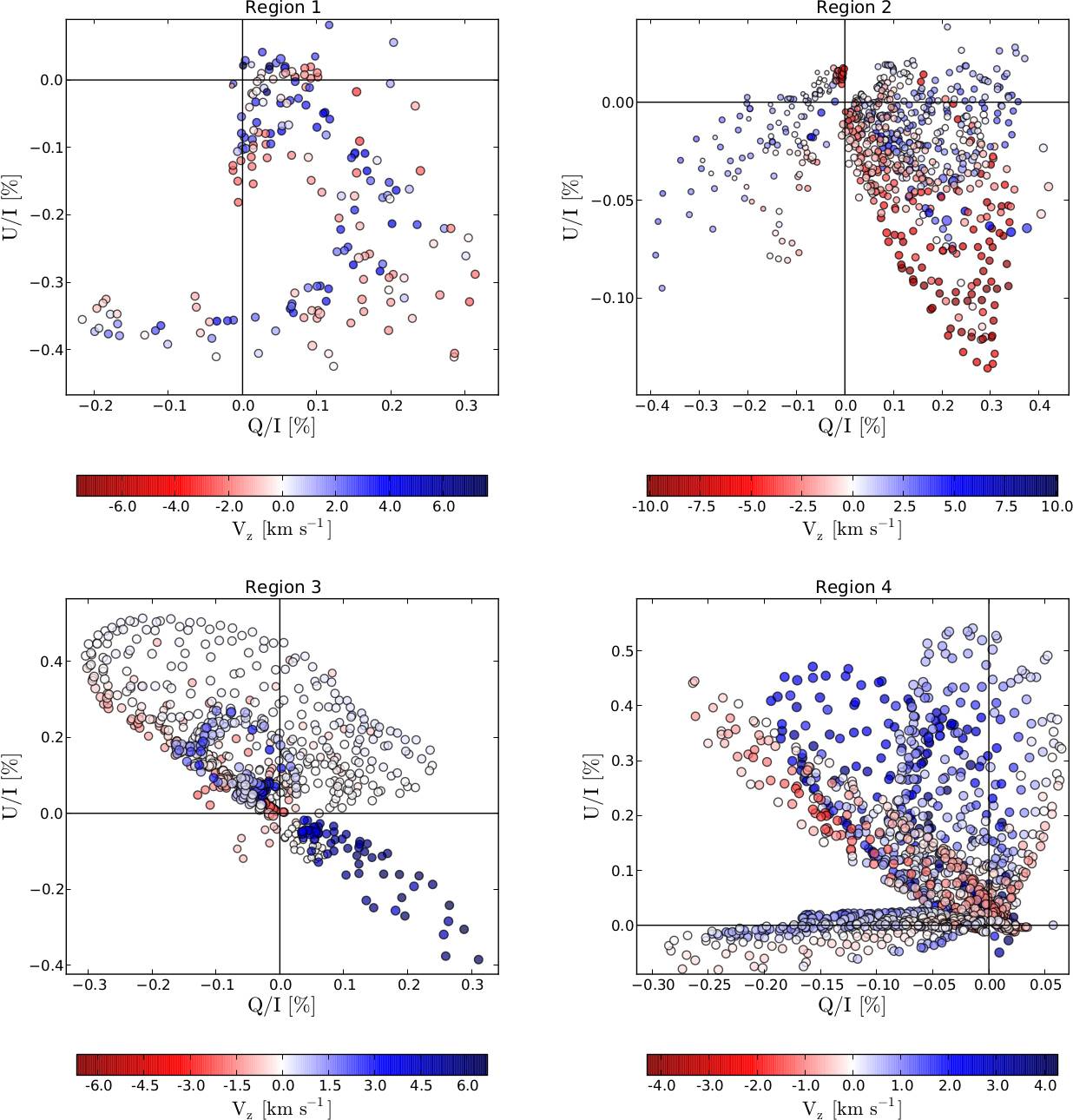
Figure A.11: The same as in Fig. 6.33, but in the K line.

A.5 Stereographic view of a cool chromospheric bubble.

Figure A.12: Stereographic representation of a cool bubble (semitransparent volume). The vertical plane shows the temperature variation (darker brown is cooler). The corrugated surface maps the heights where $\tau=1$ and its colour represents the emergent Q$/$I in the $8542$ Å line (darker blue means smaller Q$/$I). The corrugated surface sketched with polygons represents the heights of $\tau=1$ for the K line. Cyan-red glasses are required to see this figures correctly. Two-dimensional versions in next page.

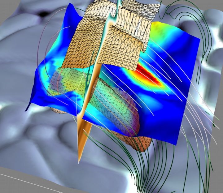
Figure A.13: Non-stereographic visualization of a cool bubble (see the caption of the previous figure). The existence of such a cool chromospheric volume is tight to the depression in the formation layer of the considered spectral line. In the borders of the region, it can be appreciated that the linear polarization tends to vanish, so drawing a thermodynamic Hanle PIL. As explained in Chapter 6, this is in part favoured by the illumination of the K line from upper layers (polygonal surface) and by the so different physical conditions existing between verticals inside and outside the bubble.

Agradecimientos

Tal vez el lector comparta la idea de que es importante sentirse inspirado para vivir con plenitud. No me refiero sólo a la inspiración científica sino también a esa “inspiración vital” que nos da impulso para evolucionar, para dar pasos cruciales en direcciones nuevas tanto en lo pequeño como en lo profundo. Una vía de inspiración insustituible es la que podemos obtener de otras personas que, con su manera de ser, sus virtudes y defectos, nos impulsan a ser la mejor versión de nosotros mismos. Inspirar a otros es más fácil cuando primero aprendemos a dejarnos inspirar; por cada sutileza, por cada gesto o palabra, por personas cercanas y también lejanas. Lo veo casi como una maestría. Esto tiene un indiscutible valor personal que no se suele apreciar, pero que recalco aquí para expresar mi gratitud y hacer partícipes a todas las personas que de alguna manera me han inspirado y dado fuerzas durante estos largos años de tesis.

En primer lugar agradezco a Andrés Asensio Ramos y a Javier Trujillo Bueno, co-autores y directores de esta tesis, la inestimable oportunidad que me han dado para formarme y aprender a su lado. Les agradezco la ilusión que pusieron en tenerme como estudiante, la energía y experiencia que han empleado en revisar nuestros trabajos, el esfuerzo que han puesto siempre en atenderme y el calvario que debe suponer tenerme como “preguntón” oficial a jornada completa. Me han enseñado mucho. Además, quiero agradecer a Andrés el apoyo en mis primeros pasos como investigador con la beca de verano del IAC. Fue precisamente con ese trabajo que también pude colaborar e interaccionar con Arturo López Ariste y Rafael Manso. Agradezco nuestras conversaciones sobre física y otros “desvaríos” de la mente científica, el apoyo recibido por Arturo y la gran ayuda que me ha supuesto contar con la constructiva crítica de Rafa para orientar mis líneas de discurso científico a favor del campo (magnético y no magnético). Gracias Rafa por ayudar a sentar las bases de trabajo sobre las que se sustenta esta tesis y por contribuir significativamente a su mejora. Ha sido también una suerte y un honor poder contar con los conocimientos y la inspiradora cercanía de Fernando Moreno, Manolo Collados y Basilio Ruiz Cobo, ya desde las clases en la universidad. Gracias a todos.

Damian Fabbian y Nacho Trujillo, amigos y compañeros de la vida, gracias por estar ahí. Gracias Damian por los intercambios de ideas sobre cómo lograr un mundo mejor. Gracias Nacho por tu amistad, por compartir tu conocimiento y por mantenerme en contacto con la investigación mientras me debatía “entre la vida y la muerte” con la gata de Schrödinger. Gracias por nuestros diálogos sobre la única revolución esencial, la de la mente y la psique.

Gracias Nayra Rodríguez (siempre tan positiva). Gracias Karla Peña (vecina, por fin!, gracias por tu apoyo). Gracias Sebas (eres un ejemplo a seguir). Gracias Carlos (siempre dispuesto a ayudar!). Gracias Mireia (no diré la palabra “miau”). Gracias Christoph Kuckein (hang loose!). Gracias Manu. Gracias Judith Bakos. Gracias Anneta (Houston…hemos dejado de tener un problema…cambio). Gracias Fernando Buitrago. Gracias Nazaret Bello. Gracias Ariadna. Gracias Peter y Jorge Pérez Prieto por presentarme a Mr. Python. Gracias a todos por la inspiración compañeros.

Me prometí que sería breve pero no va a poder ser. Estoy especialmente agradecido a Carlos Marrero, Sabrina Ruiz Marcos, Paloma García Lijó y Marián Vega, por haber sido tan buenos amigos y mantenerme presente aún en la distancia. Gracias Miguel Núñez por salvarme de una lumbalgia asegurada. Gracias Mari Carmen Trujillo por tu positividad y por tus exquisitos platos. Thank you Sowmya Krishnamurthy for the scientific discussions and for your poppy seeds dessert recipe :D. I am also very grateful to the IRSOL staff for the support.

Muchas gracias a mi familia por hacer también suyas mis penas y mis alegrías y por creer en mí. Gracias a mis padres, Melina Ramírez y Jose Manuel Carlin, y a mi querida hermana Noa. Gracias Julián, gracias Dafnis, gracias Ata, gracias Cesi. Esto está especialmente dedicado a todos ustedes.

Para finalizar quiero dar las gracias a alguien muy especial sin la que este trabajo se me hubiera hecho casi imposible. Gracias por inspirarme, por formar parte de esto y por darme razones para quedarme con la parte buena de las cosas. Literalmente tienes la última palabra en esta tesis, qué mejor final que ése: gracias Camelia!

References

- Allen Gary & Hagyard (1990) Allen Gary, G., & Hagyard, M. J. 1990, Sol. Phys., 126, 21
- Asensio Ramos (2004) Asensio Ramos, A. 2004, PhD thesis, Universidad de La Laguna, La Laguna
- Asensio Ramos et al. (2008) Asensio Ramos, A., Trujillo Bueno, J., & Landi Degl’Innocenti, E. 2008, ApJ, 683, 542
- Asplund et al. (2000) Asplund, M., Ludwig, H. G., Nordlund, A., & Stein, R. F. 2000, A&A, 359, 669
- Athay & Thomas (1961) Athay, R. G., & Thomas, R. N. 1961, Physics of the solar chromosphere (New York: Interscience Publication)
- Auer (1987) Auer, L. H. 1987, Numerical Radiative Transfer (UK: Cambridge University Press), 101
- Ayres et al. (2009) Ayres, T., H., U., G., C., K., R., T., B., Schrijver, B., D., P., J., S., M., S., W., & Solanki, S. 2009, Astro2010 Decadal Survey
- Ayres (1979) Ayres, T. R. 1979, ApJ, 228, 509
- Babcock (1947) Babcock, H. W. 1947, ApJ, 105, 105
- Baron et al. (2012) Baron, E., Hauschildt, P. H., Chen, B., & Knop, S. 2012, A&A, 548, A67
- Belluzzi et al. (2013) Belluzzi, L., Landi Degl’Innocenti, E., & Trujillo Bueno, J. 2013, A&A, 552, A72
- Belluzzi et al. (2007) Belluzzi, L., Trujillo Bueno, J., & Landi Degl’Innocenti, E. 2007, ApJ, 666, 588
- Bernes (1979) Bernes, C. 1979, A&A, 73, 67
- Blum (1981) Blum, K. 1981, Density Matrix, Theory and Applications (Plenum Press, New York and London)
- Bommier (1997) Bommier, V. 1997, A&A, 328, 706
- Bommier & Sahal-Bréchot (1978) Bommier, V., & Sahal-Bréchot, S. 1978, A&A, 69, 57
- Born & Wolf (1980) Born, M., & Wolf, E. 1980, Principles of Optics: Electromagnetic Theory of Propagation of Light (Oxford: Pergamon Press)
- Brink & Satchler (1968) Brink, D. M., & Satchler, G. R. 1968, Angular Momentum (Oxford University Press)
- Cannon (1985) Cannon, C. 1985, The transfer of spectral line radiation. (New York: Cambridge University Press)
- Cannon (1973) Cannon, C. J. 1973, ApJ, 185, 577
- Carlin et al. (2013) Carlin, E. S., Asensio Ramos, A., & Trujillo Bueno, J. 2013, ApJ, 764, 40
- Carlin et al. (2012) Carlin, E. S., Manso Sainz, R., Asensio Ramos, A., & Trujillo Bueno, J. 2012, ApJ, 751, 5
- Carlsson & Stein (1997) Carlsson, M., & Stein, R. F. 1997, ApJ, 481, 500
- Carlsson & Stein (2002) Carlsson, M., & Stein, R. F. 2002, in SOHO-11: From Solar Minimum to Maximum, ed. A. Wilson (ESA SP-508; Noordwijk: ESA)
- Casini & Landi Degl’Innocenti (2007) Casini, R., & Landi Degl’Innocenti, E. 2007, in Plasma Polarization Spectroscopy, ed. T. Fujimoto & A. Iwamae (Heidelberg:Springer), 247
- Cauzzi et al. (2008) Cauzzi, G., Reardon, K. P., Uitenbroek, H., Cavallini, F., Falchi, A., Falciani, R., Janssen, K., Rimmele, T., Vecchio, A., & Wöger, F. 2008, A&A, 480, 515
- Charbonneau (2010) Charbonneau, P. 2010, Solar and Stellar Dynamos in Magnetic Fields of Stars: From the Sun to Compact Objects (Swiss Society of Astronomy and Astrophysics)
- Collados et al. (2013) Collados, M., Bettonvil, F., Cavaller, L., Ermolli, I., Gelly, B., Pérez, H., A. .-N., Soltau, D., Volkmer, R., & EST Team. 2013, in Highlights of Spanish Astrophysics VII, 808–819
- Collados et al. (2003) Collados, M., Trujillo Bueno, J., & Asensio Ramos, A. 2003, in Astronomical Society of the Pacific Conference Series, Vol. 307, Solar Polarization, ed. J. Trujillo-Bueno & J. Sanchez Almeida, 468
- Cuperman et al. (1993) Cuperman, S., Li, J., & Semel, M. 1993, A&A, 268, 749
- de la Cruz Rodríguez & Socas-Navarro (2011) de la Cruz Rodríguez, J., & Socas-Navarro, H. 2011, A&A, 527, L8
- De la Cruz Rodríguez et al. (2012) De la Cruz Rodríguez, J., Socas-Navarro, H., Carlsson, M., & Leenaarts, J. 2012, Astronomy and Astrophysics, 543, 34
- de Pontieu et al. (2007) de Pontieu, B., McIntosh, S. W., Hansteen, V., & Carlsson, M. P. 2007, AGU Fall Meeting Abstracts, C8
- Derouich & Sahal-Bréchot (2003) Derouich, M., & Sahal-Bréchot, S. 2003, in Astronomical Society of the Pacific Conference Series, Vol. 307, Solar Polarization, ed. J. Trujillo-Bueno & J. Sanchez Almeida, 270
- Díaz et al. (1983) Díaz, A., Klkuchl, N., & Taylor, J. E. 1983, Computer Methods in Applied Mechanics and Engineering.
- Drake & Linsky (1983) Drake, S. A., & Linsky, J. L. 1983, ApJ, 273, 299
- Fabas et al. (2011) Fabas, N., Lèbre, A., & Gillet, D. 2011, A&A, 535, A12
- Fabiani Bendicho et al. (1997) Fabiani Bendicho, P., Trujillo Bueno, J., & Auer, L. H. 1997, A&A, 324, 161
- Fontenla et al. (1993) Fontenla, J. M., Avrett, E. H., & Loeser, R. 1993, ApJ, 406, 319
- Fossum & Carlsson (2005) Fossum, A., & Carlsson, M. 2005, ApJ, 625, 556
- Georgoulis (2005) Georgoulis, M. K. 2005, ApJ, 629, L69
- Guo & Babûska (1986) Guo, B., & Babûska, I. 1986, Computational Mechanics, 1, 203
- Hackbusch (1985) Hackbusch, W. 1985, Multi-Grid Methods and Applications (Springer-Verlag, Berlin)
- Hale (1908) Hale, G. E. 1908, Contributions from the Mount Wilson Observatory / Carnegie Institution of Washington, 30, 1
- Hale & Adams (1909) Hale, G. E., & Adams, W. S. 1909, Contributions from the Mount Wilson Observatory / Carnegie Institution of Washington, 41, 1
- Hale & Ellerman (1904) Hale, G. E., & Ellerman, F. 1904, ApJ, 19, 41
- Hanle (1924) Hanle, W. 1924, Z. Phys., 30, 93, [An english version exists in Moruzzi & Strumia (1991).]
- Hansteen et al. (2007) Hansteen, V. H., Carlsson, M., & Gudiksen, B. 2007, in Astronomical Society of the Pacific Conference Series, Vol. 368, The Physics of Chromospheric Plasmas, ed. P. Heinzel, I. Dorotoviĉ, & R. J. Rutten, 107
- Hansteen et al. (2006) Hansteen, V. H., De Pontieu, B., Rouppe van der Voort, L., van Noort, M., & Carlsson, M. 2006, ApJ, 647, L73
- Harvey (1969) Harvey, J. 1969, PhD thesis, University of Colorado, Boulder
- Harvey (2009) Harvey, J. 2009, in Solar Polarization 5, ed. S. Berdyugina, K. Nagendra, & R. Ramelli, ASP Conference Series (San Francisco: Astronomical Society of the Pacific), 157
- Henney et al. (2009) Henney, C. J., Keller, C. U., Harvey, J. W., Georgoulis, M. K., Hadder, N. L., Norton, A. A., Raouafi, N.-E., & Toussaint, R. M. 2009, in Astronomical Society of the Pacific Conference Series, Vol. 405, Solar Polarization 5: In Honor of Jan Stenflo, ed. S. V. Berdyugina, K. N. Nagendra, & R. Ramelli, 47
- Hubeny & Lanz (1992) Hubeny, I., & Lanz, T. 1992, A&A, 262, 501
- Hummer & Rybicki (1968) Hummer, D. G., & Rybicki, G. B. 1968, ApJ, 153, L107
- Jefferies et al. (1989) Jefferies, J., Lites, B. W., & Skumanich, A. 1989, ApJ, 343, 920
- Judge (2006) Judge, P. 2006, in Astronomical Society of the Pacific Conference Series, Vol. 354, Solar MHD Theory and Observations: A High Spatial Resolution Perspective, ed. J. Leibacher, R. F. Stein, & H. Uitenbroek, 259
- Judge (2010) Judge, P. G. 2010, Mem. Soc. Astron. Italiana, 81, 543
- Judge & Carlsson (2010) Judge, P. G., & Carlsson, M. 2010, ApJ, 719, 469
- Keller et al. (2003) Keller, C. U., Harvey, J. W., Henney, C. J., & Jones, H. P. 2003, in IAU Joint Discussion, Vol. 3, IAU Joint Discussion
- Kunasz & Auer (1988) Kunasz, P., & Auer, L. H. 1988, J. Quant. Spectrosc. Radiat. Transfer, 39, 67
- Kurucz et al. (1984) Kurucz, R. L., Furenlid, I., Brault, J., & Testerman, L. 1984, Solar flux atlas from 296 to 1300 nm
- Lamb & Ter Haar (1971) Lamb, F. K., & Ter Haar, D. 1971, Phys. Rep., 2, 253
- Landi Degl’Innocenti (1984) Landi Degl’Innocenti, E. 1984, Sol. Phys., 91, 1
- Landi Degl’Innocenti & Bommier (1993) Landi Degl’Innocenti, E., & Bommier, V. 1993, ApJ, 411, L49
- Landi Degl’Innocenti & Landi Degl’Innocenti (1977) Landi Degl’Innocenti, E., & Landi Degl’Innocenti, M. 1977, A&A, 56, 111
- Landi Degl’Innocenti & Landolfi (2004) Landi Degl’Innocenti, E., & Landolfi, M. 2004, Polarization in Spectral Lines (Kluwer Academic Publishers)
- Landolfi & Landi Degl’Innocenti (1996) Landolfi, M., & Landi Degl’Innocenti, E. 1996, Sol. Phys., 164, 191
- Leenaarts et al. (2009a) Leenaarts, J., Carlsson, M., Hansteen, V., & Rouppe van der Voort, L. 2009a, ApJ, 694, L128
- Leenaarts et al. (2009b) —. 2009b, ApJL, 694, L128
- Leka & Metcalf (2003) Leka, K. D., & Metcalf, T. R. 2003, Sol. Phys., 212, 361
- Linsky & Avrett (1970) Linsky, J. L., & Avrett, E. H. 1970, PASP, 82, 169
- Lites et al. (1993) Lites, B. W., Rutten, R. J., & Kalkofen, W. 1993, ApJ, 414, 345
- López Ariste (2001) López Ariste, A. 2001, in Astronomical Society of the Pacific Conference Series, Vol. 248, Magnetic Fields Across the Hertzsprung-Russell Diagram, ed. G. Mathys, S. K. Solanki, & D. T. Wickramasinghe, 621
- Lucy (1971) Lucy, L. B. 1971, ApJ, 163, 95
- Lucy (2005) —. 2005, A&A, 429, 19
- Manso Sainz (2002) Manso Sainz, R. 2002, PhD thesis, Universidad de La Laguna, La Laguna
- Manso Sainz & Landi Degl’Innocenti (2002) Manso Sainz, R., & Landi Degl’Innocenti, E. 2002, A&A, 394, 1093
- Manso Sainz et al. (2004) Manso Sainz, R., Landi Degl’Innocenti, E., & Trujillo Bueno, J. 2004, ApJL, 614, L89
- Manso Sainz & Trujillo Bueno (2003a) Manso Sainz, R., & Trujillo Bueno, J. 2003a, Physical Review Letters, 91, 111102
- Manso Sainz & Trujillo Bueno (2003b) Manso Sainz, R., & Trujillo Bueno, J. 2003b, in Astronomical Society of the Pacific Conference Series, Vol. 307, Solar Polarization, ed. J. Trujillo-Bueno & J. Sanchez Almeida, 251
- Manso Sainz & Trujillo Bueno (2010) —. 2010, ApJ, 722, 1416
- McCrea (1929) McCrea, W. H. 1929, Nature, 124, 442
- Metcalf (1994) Metcalf, T. R. 1994, Sol. Phys., 155, 235
- Metcalf et al. (2006a) Metcalf, T. R., Leka, K. D., Barnes, G., Lites, B. W., Georgoulis, M. K., Pevtsov, A. A., Balasubramaniam, K. S., Gary, G. A., Jing, J., Li, J., Liu, Y., Wang, H. N., Abramenko, V., Yurchyshyn, V., & Moon, Y.-J. 2006a, Sol. Phys., 237, 267
- Metcalf et al. (2006b) —. 2006b, Sol. Phys., 237, 267
- Mihalas (1978) Mihalas, D. 1978, in Stellar Atmospheres, Vol. 455
- Mihalas & Kunasz (1986) Mihalas, D., & Kunasz, P. 1986, 64, 1
- Milne (1924) Milne, E. A. 1924, MNRAS, 85
- Molodij & Bommier (2011) Molodij, G., & Bommier, V. 2011, in IAU Symposium, Vol. 274, IAU Symposium, ed. A. Bonanno, E. de Gouveia Dal Pino, & A. G. Kosovichev, 291–294
- Moon et al. (2003) Moon, Y.-J., Wang, H., Spirock, T., Goode, P., & Park, Y. 2003, Solar Phys., 217, 79
- Nagendra (1996) Nagendra, K. N. 1996, Sol. Phys., 164, 67
- Omont et al. (1973) Omont, A., Smith, E. W., & Cooper, J. 1973, ApJ, 182, 283
- Parker (1994) Parker, E. N. 1994, Spontaneous current sheets in magnetic fields : with applications to stellar x-rays. International Series in Astronomy and Astrophysics, Vol. 1. New York : Oxford University Press, 1994., 1
- Parker (2007) —. 2007, Conversations on Electric and Magnetic Fields in the Cosmos (Princeton University Press)
- Parker (1989) Parker, S. B. 1989, McGraw-Hill Dictionary of Scientific and Technical Terms (4th ed.) No. ISBN 0-07-045270-9 (New York: McGraw-Hill.)
- Pietarila et al. (2009) Pietarila, A., Hirzberger, J., Zakharov, V., & Solanki, S. K. 2009, A&A, 502, 647
- Racah (1942) Racah, G. 1942, 62, 438
- Ramachandran & Varoquaux (2011) Ramachandran, P., & Varoquaux, G. 2011, IEEE Computing in Science Engineering, 40
- Ramelli et al. (2010) Ramelli, R., Balemi, S., Bianda, M., Defilippis, I., Gamma, L., Hagenbuch, S., Rogantini, M., Steiner, P., & Stenflo, J. O. 2010, 77351Y
- Reardon et al. (2009) Reardon, K. P., Uitenbroek, H., & Cauzzi, G. 2009, A&A, 500, 1239
- Rees & Guo (2003) Rees, D., & Guo, Y. 2003, in Astronomical Society of the Pacific Conference Series, Vol. 307, Solar Polarization, ed. J. Trujillo-Bueno & J. Sanchez Almeida, 85
- Rees et al. (1989) Rees, D. E., Durrant, C. J., & Murphy, G. A. 1989, ApJ, 339, 1093
- Rees et al. (2000) Rees, D. E., López Ariste, A., Thatcher, J., & Semel, M. 2000, A&A, 355, 759
- Rimmele et al. (2013) Rimmele, T., Berger, T., McMullin, J., Keil, S., Goode, P., Knoelker, M., Kuhn, J., Rosner, R., Casini, R., Lin, H., Woeger, F., von der Luehe, O., Tritschler, A., & Atst Team. 2013, in EGU General Assembly Conference Abstracts, Vol. 15, EGU General Assembly Conference Abstracts, 6305
- Ruiz Cobo & del Toro Iniesta (1994) Ruiz Cobo, B., & del Toro Iniesta, J. C. 1994, A&A, 283, 129
- Rutten (2003) Rutten, R. J. 2003, Radiative Transfer in Stellar Atmospheres (Utrecht University)
- Rybicki & Hummer (1991) Rybicki, G. B., & Hummer, D. G. 1991, A&A, 249, 720
- Sánchez Almeida et al. (1989) Sánchez Almeida, J., Collados, M., & del Toro Iniesta, J. C. 1989, A&A, 222, 311
- Scherrer et al. (2012) Scherrer, P., Schou, J., Bush, R., Kosovichev, A., Bogart, R., Hoeksema, J., Liu, Y., Duvall, T.L., J., Zhao, J., Title, A., Schrijver, C., Tarbell, T., & Tomczyk, S. 2012, Solar Physics, 275, 207
- Shimizu et al. (2011) Shimizu, T., Tsuneta, S., Hara, H., Ichimoto, K., Kusano, K., Sakao, T., Sekii, T., Suematsu, Y., & Watanabe, T. 2011, in Society of Photo-Optical Instrumentation Engineers (SPIE) Conference Series, Vol. 8148, Society of Photo-Optical Instrumentation Engineers (SPIE) Conference Series
- Skumanich & Semel (1996) Skumanich, A., & Semel, M. 1996, Sol. Phys., 164, 291
- Sobelman (1973) Sobelman, I. I. 1973, An introduction to the theory of atomic spectra. (Pergamon Press)
- Sobolev (1958) Sobolev, V. V. 1958, Theoretical Astrophysics (London: Pergamon Press Ltd.)
- Sobolev (1960) —. 1960, Moving Envelopes of stars (Harvard University Press)
- Socas-Navarro (2001) Socas-Navarro, H. 2001, in Advanced Solar Polarimetry: Theory, Observation and Instrumentation, ed. K. N. Nagendra & J. O. Stenflo, ASP Conf. Series, Kluwer Academic Publishers, Vol. 236, 487
- Socas-Navarro et al. (2006) Socas-Navarro, H., Elmore, D., Pietarila, A., Darnell, A., Lites, B. W., Tomczyk, S., & Hegwer, S. 2006, Sol. Phys., 235, 55
- Socas-Navarro & Trujillo Bueno (1997) Socas-Navarro, H., & Trujillo Bueno, J. 1997, ApJ, 490, 383
- Socas-Navarro et al. (2000) Socas-Navarro, H., Trujillo Bueno, J., & Ruiz Cobo, B. 2000, ApJ, 530, 977
- Socas-Navarro & Uitenbroek (2004) Socas-Navarro, H., & Uitenbroek, H. 2004, ApJ, 603, L129
- Spiegel (1998) Spiegel, M. & Liu, J. 1998, tablas1998 (Ed. McGraw-Hill)
- Stein & Nordlund (1998) Stein, R. F., & Nordlund, A. 1998, ApJ, 499, 914
- Stenflo (1978) Stenflo, J. O. 1978, A&A, 66, 241
- Stenflo (1994) —. 1994, Solar Magnetic Fields. Polarized Radiation Diagnostics (Dordrecht: Kluwer Academic Publishers)
- Stenflo (2006) Stenflo, J. O. 2006, in Astronomical Society of the Pacific Conference Series, Vol. 358, Astronomical Society of the Pacific Conference Series, ed. R. Casini & B. W. Lites, 215
- Stenflo (2013) —. 2013, Polarimetry of the Sun, Vol. Planets, Stars and Nebulae studied with Photopolarimetry (Cambridge University Press)
- Stenflo et al. (1998) Stenflo, J. O., Keller, C. U., & Gandorfer, A. 1998, A&A, 329, 319
- Stenflo et al. (2000) —. 2000, A&A, 355, 789
- Stenflo et al. (1983) Stenflo, J. O., Twerenbold, D., & Harvey, J. W. 1983, A&AS, 52, 161
- Ŝtêpán & Trujillo Bueno (2010) Ŝtêpán, J., & Trujillo Bueno, J. 2010, Mem. Soc. Astron. Italiana, 81, 810
- Ŝtêpán & Trujillo Bueno (2013) Ŝtêpán, J., & Trujillo Bueno, J. 2013, A&A, 557, A143
- Süli (2012) Süli, E. 2012, lecture notes.
- Trujillo Bueno (1999) Trujillo Bueno, J. 1999, in Solar Polarization, ed. K. N. Nagendra & J. O. Stenflo, Kluwer Academic Publishers, 73–96
- Trujillo Bueno (2001) Trujillo Bueno, J. 2001, in Astronomical Society of the Pacific Conference Series, Vol. 236, Advanced Solar Polarimetry – Theory, Observation, and Instrumentation, ed. M. Sigwarth, 161
- Trujillo Bueno (2003a) Trujillo Bueno, J. 2003a, in Modeling of Stellar Atmospheres, ed. N. E. Piskunov, W. W. Weiss, & D. F. Gray, IAU Symposium 210 (ASP Conf. Ser.), 243
- Trujillo Bueno (2003b) Trujillo Bueno, J. 2003b, in Solar Polarization 3, ed. J. Trujillo Bueno & J. Sánchez Almeida, ASP Conf. Ser. Vol 307, 407
- Trujillo Bueno (2003c) Trujillo Bueno, J. 2003c, in Stellar Atmosphere Modeling, ed. I. Hubeny, D. Mihalas, & K. Werner, ASP Conf. Ser. 288 (San Francisco: ASP), 551
- Trujillo Bueno (2010) Trujillo Bueno, J. 2010, in Magnetic Coupling between the Interior and Atmosphere of the Sun, ed. S. S. Hasan & R. J. Rutten, 118
- Trujillo Bueno et al. (2001) Trujillo Bueno, J., Collados, M., Paletou, F., & Molodij, G. 2001, in ASP Conf. Ser. 236: Advanced Solar Polarimetry – Theory, Observation, and Instrumentation, ed. M. Sigwarth, 141
- Trujillo Bueno & Fabiani Bendicho (1995) Trujillo Bueno, J., & Fabiani Bendicho, P. 1995, ApJ, 455, 646
- Trujillo Bueno & Manso Sainz (1999) Trujillo Bueno, J., & Manso Sainz, R. 1999, apj, 516, 436
- Trujillo Bueno et al. (2004) Trujillo Bueno, J., Shchukina, N., & Asensio Ramos, A. 2004, Nature, 430, 326
- Tsuneta et al. (2008) Tsuneta, S., Ichimoto, K., Katsukawa, Y., Nagata, S., Otsubo, M., Shimizu, T., Suematsu, Y., Nakagiri, M., Noguchi, M., Tarbell, T., Title, A., Shine, R., Rosenberg, W., Hoffmann, C., Jurcevich, B., Kushner, G., Levay, M., Lites, B., Elmore, D., Matsushita, T., Kawaguchi, N., Saito, H., Mikami, I., Hill, L. D., & Owens, J. K. 2008, Sol. Phys., 249, 167
- Turk & Pentland (1991) Turk, M. A., & Pentland, A. P. 1991, in Society of Photo-Optical Instrumentation Engineers (SPIE) Conference Series, Vol. 1381, Society of Photo-Optical Instrumentation Engineers (SPIE) Conference Series, ed. D. P. Casasent, 43–54
- Uitenbroek (1989) Uitenbroek, H. 1989, A&A, 213, 360
- Uitenbroek (2001) —. 2001, ApJ, 557, 389
- Uitenbroek (2002) —. 2002, ApJ, 565, 1312
- Uitenbroek (2006) Uitenbroek, H. 2006, in Astronomical Society of the Pacific Conference Series, Vol. 354, Solar MHD Theory and Observations: A High Spatial Resolution Perspective, ed. J. Leibacher, R. F. Stein, & H. Uitenbroek, 313
- Uitenbroek (2011) Uitenbroek, H. 2011, in Astronomical Society of the Pacific Conference Series, Vol. 437, Solar Polarization 6, ed. J. R. Kuhn, D. M. Harrington, H. Lin, S. V. Berdyugina, J. Trujillo-Bueno, S. L. Keil, & T. Rimmele, 439
- Unno (1956) Unno, W. 1956, Pub. Astr. Soc. Japan, 8, 108
- Vecchio et al. (2009) Vecchio, A., Cauzzi, G., & Reardon, K. P. 2009, A&A, 494, 269
- Vecchio et al. (2007) Vecchio, A., Cauzzi, G., Reardon, K. P., Janssen, K., & Rimmele, T. 2007, A&A, 461, L1
- Wedemeyer et al. (2004) Wedemeyer, S., Freytag, B., Steffen, M., Ludwig, H.-G., & Holweger, H. 2004, A&A, 414, 1121
- Wesseling (1995) Wesseling, P. 1995, Introduction to Multigrid Methods (ICASE, NASA)
- Young (1862) Young, C. 1862, Popular Science Monthly/Volume 4/February 1874/The Chromosphere and Solar Prominences — Wikisource,