Multiple Ionization of Neon under soft x-rays: Theory vs Experiment

Abstract

We present a rather elaborate theoretical model describing the dynamics of Neon under radiation of photon energies $\sim 93$ eV and pulse duration in the range of 15 fs, within the framework of Lowest non-vanishing Order of Perturbation Theory (LOPT), cast in terms of rate equations. Our model includes sequential as well as direct multiple ionization channels from the 2s and 2p atomic shells, including aspects of fine structure, whereas the stochastic nature of SASE-FEL light pulses is also taken into account. Our predictions for the ionization yields of the different ionic species are in excellent agreement with the related experimental observations at FLASH.

1 Introduction

In a 2011 paper [LamPRA11], we explored the conditions under which direct multiple ionization channels might make significant contribution to ionic yields, which are usually dominated by the inevitably present sequential channels. In order to present a quantitative assessment, we had chosen the Neon atom driven by radiation of photon energy 93 eV, of pulse intensity and duration available at present day Free-Electron Laser (FEL) facilities such as FLASH [Ack07, richter]. Our choice was motivated in part by related experimental data obtained under the above mentioned conditions [richter, richter09]. Since the chief objective of our study was the evaluation of direct multiple ionization in comparison to the sequential contributions, we focused our model on the ionization of outer subshell (2p) electrons, although a complete theoretical description would have required the inclusion of single-photon ionization of 2s electrons as well. This means that we were evaluating the relative importance of direct multiple ionization from the 2p subshell alone. In a sense, our work could be viewed as a numerical experiment. At the time of that work, we were aware of only TOF (Time of Flight) data [richter09] which we did consider in the spirit of a qualitative comparison with our calculations; because extracting ionic yields from a figure showing TOF spikes only is highly problematic. Given its limited scope, that comparison was nevertheless compatible with our results, in the sense that under the parameters of that experiment (in particular the pulse duration), we did not expect a discernible presence of contributions from the direct channels; and indeed none was found in the experimental data. It did, however, transpire that direct multielectron channels can begin competing with the sequential ones only when the duration of the pulse falls below 5 fs or so.

In a most recent paper by Guichard et al. [Guichard13] addressing the same problem, the authors have presented a quantitative interpretation of the experimental data pertaining to the above mentioned experiment, including this time laser intensity dependences of the ionic yields. This new piece of experimental evidence behoves us to test our approach in a suitably more elaborate model. The approach in Ref. [Guichard13] relies on a rather simplified model, referred to by the authors as “minimal model”, in terms of which a good fit to the experimental data was obtained. That fit was compared (see Fig.3 of Ref. [Guichard13]) to what our equations would have given. Not surprisingly, our equations lead to ionic yields systematically lower than the experimental data. That was to be expected since, for the reasons outlined above, the single-photon ionization channels of the 2s electrons had not been taken into account in [LamPRA11]. Moreover, in [Guichard13] the authors compared the experimental data to our results of Ref. [LamPRA11], for a Fourier-limited pulse duration of 30 fs, which however is considerably longer than the estimated pulse duration in the experiment i.e., $15\pm 5$ fs.

Since the term “minimal model” may be open to a variety of interpretations, it is important to state and discuss here clearly the main assumptions underlying the model of Ref. [Guichard13]. The formalism rests on a set of rate equations governing the production and depletion of the ionic yields during the pulse. For the photon energy, range of intensities and pulse duration employed in the experiment, the rate equations are perfectly valid (e.g., see discussion in [LamPRA11, makris09, LamNik13]). The distribution of the laser intensity within the interaction volume, as determined by the focusing geometry of the laser beam, has been taken into account. Presumably, the term “minimal model” has to do with the following additional assumptions/approximations adopted by the authors: (a) Only sequential channels were included in the rate equations. (b) The field (intensity) fluctuations, inherent in SASE FELs, and specifically FLASH pulses [Ack07, richter, Mitz08-09], were not included in the calculations. (c) All ionic species were assumed to be produced by single-photon ionization. (d) All of the single-photon cross sections entering the model were assumed to have the same value.

If the purpose of the work in [Guichard13] was to obtain a fit to the data, it appears that it has succeeded reasonably well, for the ionic species up to Ne⁴⁺. However, in order to understand the physical meaning of the fit, we need to examine the validity of the underlying assumptions/approximations. Approximation (a) above is justified, because the direct channels, being of much higher order of non-linearity, are expected to begin competing with the sequential only for quite short pulses; say below 5 fs, as demonstrated in [LamPRA11]. Approximation (b) may be useful in assessing some general features of the data, but the results may at times be misleading. Approximations (c) and (d), however, are quite problematic. The difficulty stems from the fact that the rate equations, which bears repeating are perfectly valid in this context, imply energy conservation in terms of number of photons absorbed in each transition and the corresponding ionization threshold. This is a condition inherent in the notion of the cross section. Thus, as discussed in detail below, although ions up to Ne⁴⁺ are produced mainly in a sequence of single-photon absorptions, from there on it is only two- and three-photon processes that enter the sequence of allowed transitions. In the absence of those channels, ionic species beyond Ne⁴⁺ cannot be populated through energy conserving processes. Inserting single-photon cross sections for those species and adjusting parameters may of course produce populations for those species, but the underlying process is devoid of physical meaning.

Coming now to the present formulation, the main addition to our earlier paper [LamPRA11] is the detailed inclusion of all single-photon channels, as well as a careful estimation of the two- and three-photon cross sections. But perhaps more importantly, accounting for the field fluctuations, is shown to be of crucial importance in the interpretation of the experimental data. As has been shown in great detail in [NikLam12-13], for a quantitative comparison with experimental data pertaining to SASE-FEL radiation, it is imperative to include a stochastic model that describes accurately the statistical properties of the pulses, pertaining to the source and the conditions of the experiment. This is an issue sufficiently important to merit further elaboration at this point. In the absence of intensity fluctuations, it is basically the laser bandwidth that matters. In that case, for a pulsed source, the effective bandwidth is determined by the combination of the Fourier and the stochastic bandwidths. But for a source with intensity fluctuations, the particular statistics underlying the fluctuations are of crucial importance. Intensity fluctuations entail a spiky temporal structure, under an envelop determined by the pulse duration and the usually present monochromator. As a consequence of the intensity fluctuations, an important parameter is the coherence time, which can be and often has been determined through the measurement of a two-photon autocorrelation function [Mitz08-09]. In essence, it provides a measure of the duration of the dominant intensity spike under the complicated spiky structure of a pulse with the stochastic properties of the SASE FEL. There is then an overall (total) bandwidth associated with this coherence time which for a Gaussian pulse and Gaussian correlated noise is given by [NikLam12-13]

$$\Delta\omega=\sqrt{\Delta\omega_{\min}^{2}+\gamma^{2}},$$ (1)

where $\Delta\omega_{\min}$ is the Fourier-limited bandwidth of the pulse and $\gamma=\sqrt{8\pi\ln(2)/T_{c}}$. In general, one cannot account for this bandwidth e.g., by simply correcting the parameters entering the equation of motion for the density matrix of the atomic system [NikLam12-13]. That is why detailed modelling of the field fluctuations is an absolutely necessary ingredient of the rate equations, which as a result are stochastic differential equations[NikLam12-13].

In the following section 2, we present a detailed discussion of the ionization channels and the respective orders of non-linearity, included in our calculations. The 1s electrons are assumed frozen because, for photon energy 93 eV and peak intensities less than $10^{16}$W/cm² the 1s electrons are too strongly bound to be affected. The details of the rate equations, including the interaction volume features are presented in section 3, followed by section 4 in which we present results without and with field fluctuations, thus demonstrating their significance in interpreting experimental data. In the last section 5, we summarize our findings as well as certain issues that remain open.

2 Ionization paths for Neon at 93eV

A concise summary of all ionization channels included in our calculations is shown in Fig. 1, listing important quantities, such as ionization potentials and the order of each transition, together with the flow of charge indicated by arrows. This “flow chart” includes ejections of electrons from both the 2s and 2p shells, where each circle corresponds to a particular ionic species with the two numbers in its lower half denoting the number of remaining electrons in the 2s and the 2p shells. This is because ionic species at different internal states appear and disappear during the ionization of neutral Neon at the particular photon energy. For example, one can see that Ne³⁺ appears in three different states, namely $\left|2s^{2},2p^{3}\right\rangle$, $\left|2s^{1},2p^{4}\right\rangle$ and $\left|2s^{0},2p^{5}\right\rangle$. As will be seen later on, in a sequential ionization process, a given ion at different internal states may lead to the same or to different internal states of the next higher ion, through substantially different cross-sections. For a quantitative comparison to experimental data, the inclusion of all of these intermediate ionic species is therefore necessary. In the following, the ion Ne^q+ in the state $\left|2s^{a},2p^{b}\right\rangle$ is denoted by Ne${}_{a,b}^{q+}$, while charge conservation implies

$$a+b=8-q\equiv\tilde{q}.$$ (2)

In view of Eq. (2), each ionic species is uniquely defined by the two labels $a$ and $b$.

Careful inspection of the “flow chart” does reveal some interesting regularities in the underlying processes, which will help us elucidate the results. More precisely, for the ions up to Ne⁴⁺ single-photon and two-photon sequential ionization channels co-exist. On the other hand, the ions Ne⁵⁺ and Ne⁶⁺ can be created only through two-photon sequential ionization, whereas three photons are required for the last two ionic species, namely, Ne⁷⁺ and Ne⁸⁺. The direct multiple ionization channels depicted in Fig. 1 lead from Ne to Ne^q+, with $q\geq 2$, and pertain to the multiphoton ejection of more than one electrons from the 2p shell of neutral Neon only, since channels that involve electron ejection from the 2s shell are expected to have considerably smaller cross sections. In principle, when energetically allowed, $n$-photon $m$-electron ejection (with $n\geq m$) can always occur from any ionic species, and actually it does not necessarily require any electron correlation. As a first approximation, however, we have included only direct ionization channels from neutral Neon, since this is mainly present for short times. Our simulations, showed that for the parameters of the experiment, the contribution of these channels was negligible and thus there was no need for including direct ionization of intermediate ions.

Finally, it should be emphasized that the “flow chart” of Fig. 1 corresponds to photon energy $93$ eV, with the ionization potentials obtained from the codes in Ref. [cowan]. The counterpart of this “flow chart” for photon energy $90.5$ eV differs only in the order of the transition Ne${}_{2,4}^{2+}\to$Ne${}_{1,4}^{3+}$, which becomes a two-photon process. In either case, it is the ratio of the cross sections for the transitions Ne${}_{2,4}^{2+}\to$Ne${}_{2,3}^{3+}$ and Ne${}_{2,4}^{2+}\to$Ne${}_{1,4}^{3+}$ that determines the dominant ionization path followed by the system. As shown in Table LABEL:tabCS, the single-photon cross-section for Ne${}_{2,4}^{2+}\to$Ne${}_{2,3}^{3+}$ at 93 eV is considerably larger than the corresponding cross-section for Ne${}_{2,4}^{2+}\to$Ne${}_{1,4}^{3+}$. Moreover, as discussed later on, the manifold of (near) resonances at 90.5 and 93 eV are very similar, and thus the relative strength of the cross sections remain practically the same. Therefore, considering either of the photon energies reported in the experiment of [Guichard13], is not expected to modify or introduce any prominent distinguishing features in the yields of Ne²⁺ and Ne³⁺, in agreement with the reported experimental data. As a result, for the sake of concreteness, our theoretical analysis has been focused on photons of energy 93 eV. As confirmed later on, our theoretical results for the laser intensity dependence of the ionic yields are in a very good agreement with those of the experiment for both 90.5 and 93 eV.

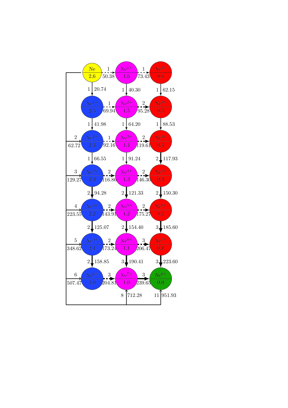
Figure 1: Ionization paths for Neon. The numbers close to each arrow denote the ionization potential in eV and the number of photons required for ionization assuming photons of energy 93 eV. Different colours (columns) denote ion species with 0, 1 and 2 holes in the 2s shell.

3 Theory vs Experiment

As discussed above, our model focuses on the populations of the ionic species up to Ne⁸⁺ and includes different sequential and direct ionization paths from both of the 2s and 2p shells. Although in the experimental data, the highest observable ionic species was Ne⁶⁺, it is necessary to include the rate equations for Ne⁷⁺ and Ne⁸⁺, because otherwise the population of Ne⁶⁺ would increase monotonically, reaching eventually the value 1, violating thus the physical reality of the experiment. Throughout our simulations, the complete set of differential equations that governs the populations of the ionic species during the pulse is the following:

-∑_b=0^4σ_2,6;2,b^(6-b) F^6-b N_2,6-σ_2,6;1,0^(8) F^8 N_2,6 -σ_2,6;0,0^(11) F^11 N_2,6 dN2,5dt &= σ_2,6;2,5^(1) F N_2,6 -σ_2,5;1,5^(1) F N_2,5 -σ_2,5;2,4^(1) F N_2,5 dN1,6dt = σ_2,6;1,6^(1) F N_2,6 -σ_1,6;0,6^(1) F N_1,6 -σ_1,6;1,5^(1) F N_1,6 dN2,4dt = σ_2,5;2,4^(1) F N_2,5+σ_2,6;2,4^(2) F^2 N_2,6 -σ_2,4;2,3^(1) F N_2,4 -σ_2,4;1,4^(1) F N_2,4 dN1,5dt =σ_2,5;1,5^(1) F N_2,5 +σ_1,6;1,5^(1) F N_1,6 -σ_1,5;1,4^(1) F N_1,5 -σ_1,5;0,5^(2) F^2 N_1,5 dN0,6dt = σ_1,6;0,6^(1) F N_1,6 -σ_0,6;0,5^(1) F N_0,6 dN2,3dt =σ_2,4;2,3^(1) F N_2,4+σ_2,6;2,3^(3) F^3 N_2,6 -σ_2,3;2,2^(2) F^2 N_2,3 -σ_2,3;1,3^(2) F^2 N_2,3 dN1,4dt =σ_2,4;1,4^(1) F N_2,4 + σ_1,5;1,4^(1) F N_1,5 -σ_1,4;1,3^(1) F N_1,4 -σ_1,4;0,4^(2) F^2 N_1,4 dN0,5dt = σ_0,6;0,5^(1) F N_0,6+σ_1,5;0,5^(2) F^2 N_1,5 -σ