TDOA–based localization in two dimensions:
the bifurcation curve

Abstract.

In this paper, we complete the study of the geometry of the TDOA map that encodes the noiseless model for the localization of a source from the range differences between three receivers in a plane, by computing the Cartesian equation of the bifurcation curve in terms of the positions of the receivers. From that equation, we can compute its real asymptotic lines. The present manuscript completes the analysis of [12]. Our result is useful to check if a source belongs or is closed to the bifurcation curve, where the localization in a noisy scenario is ambiguous.

1. Introduction

The problem of localizing an object in space is a classical topic in the literature of space–time signal processing. The first studies on the subject date back to World War II, motivating the creation of the two-dimensional LOng RAnge Navigation (LORAN) radio positioning system. LORAN was based on the measurements of the time differences of arrival (TDOA) of synchronized radio signals originated from three distinct known emitters and it required the use of hyperbolic charts to determine the position of the receiver [14].

Nowadays, LORAN has been replaced primarily by Global Positioning System (GPS), but the mathematical models underlying LORAN and (three–dimensional) GPS localization are essentially the same [27]. TDOA–based localization of unknown point sources is very widespread and popular also in acoustic signal processing, because it is characterized by a reduced computational cost with respect to other solutions and robustness against noise [18].

The main contributions to the study of TDOA–based localization come from the engineering literature, where the authors usually focus on the development of algorithms for locating the source starting from empirical TDOA data, affected by (mainly, Gaussian distributed) noise. Relevant examples are [29, 28, 2, 25, 19, 20, 18, 21, 15, 6]. A classification of the different methods can be done according to the proposed solution: maximum likelihood principle versus least–squares estimators, linear approximation versus numerical optimization, and finally iterative versus closed forms–algorithms (for a resume of the most significant of these methods see [7]).

However, all of them are based on the model of geometric propagation of the signal in an isotropic and homogeneous medium. This means that, given a TDOA measurement between two receivers placed on the Euclidean plane at positions $\mathbf{m}_{i}$ and $\mathbf{m}_{j}$, the locus of source locations that are compatible with that measurement is one branch of a hyperbola of foci $\mathbf{m}_{i}$ and $\mathbf{m}_{j}$ and whose aperture depends on the range difference (TDOA times the speed of propagation of the signal). Therefore, if we consider multiple measurements, one can readily find the location of the source through the intersection of branches of hyperbole. The three dimensional localization is very similar, being equivalent to the intersection of sheets of hyperboloids.

The mathematical properties of the TDOA–based localization have been investigated in several manuscripts. In particular, the closed–form solutions to the intersection problems have been provided for both configurations of three receivers in a plane and four receivers in the space [26, 5, 23, 1, 9, 24, 17, 16, 4, 10, 31, 11, 12]. However, due to the nonlinearity, it is well known that in these minimal configurations of receivers there does not exist a unique admissible position of the source for any given set of TDOA measurements. In fact, there are open regions in the physical space where the intersection set is the union of two points and so the source location is intrinsically ambiguous. This fact is known in literature as the bifurcation problem and we will name bifurcation set the border between the two domains where the localization problem has respectively one or two solutions.

In [26] it is shown that the bifurcation set is a curve in two dimensions and a surface in three dimensions. In [17], by relating TDOA–based localization and the ancient Problem of Apollonius [8] of drawing a circle touching three other circles or two circles and a point, Hoshen was able to analytically describe the bifurcation sets in two and three dimension in terms of polar and spherical coordinates. More recently, an analysis of the bifurcation problem in a 2–D scenario has been completed through the use of numerical simulations [30]. Source location error analysis in 2–D and 3–D with noisy TDOA data has also recently been considered for both closed form and numerical solutions [31].

A deeper description of the geometric properties of the bifurcation curve in the 2–D case was given lately by the authors in [12]. Although the statistical model describing TDOA–based localization is not defined by polynomial functions, in [12] it has been shown that all the relevant objects are real (semi)–algebraic varieties. In particular, the bifurcation curve is an algebraic curve and more precisely a rational quintic curve, whose explicit rational parametrization was provided. In [12], we were not able to find a Cartesian polynomial equation.

In this manuscript, we fill this gap by providing the explicit Cartesian equation of the bifurcation curve in terms of the positions of the receivers. This is an important step towards the study of the statistical model of localization based on TDOAs. Indeed, as observed in [12], locating a source placed around the bifurcation curve is an ill-posed problem and in these situations any localization algorithm has a very low accuracy. On the other hand, checking if a point belongs to, or is close to, a curve is quite a hard problem if one starts from the parametric equation of the curve itself. On the contrary, the two above–mentioned problems can be easily solved from the Cartesian equation of the curve.

The paper is organized as follows. In Section 2, we describe the deterministic model of the physical problem, and we recall the main results proved in [12]. Section 3 is devoted to the computation of the Cartesian equation of the bifurcation curve and of its real asymptotic lines in terms of the positions of the receivers. In the last Section, we summarize the results, and we outline a research program for extending our study to both the real scenario, and the cases not yet covered, such as the 3–D case, or the planar case with more than $3$ receivers.

2. State of the art

In this section we briefly resume the main results of [12] concerning the 2–D localization with three receivers in a noiseless scenario. In this setting, the physical world can be identified with the Euclidean plane and, after choosing an orthogonal Cartesian coordinate system, with $\mathbb{R}^{2}$. On the plane, we have three receivers $\mathbf{m_{i}}=(x_{i},y_{i}),\ i=0,1,2$ at known positions and a source $\mathbf{x}=(x,y)$.

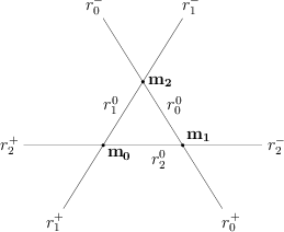
Figure 1. Receivers $\mathbf{m_{0}},\mathbf{m_{1}},\mathbf{m_{2}}$ in a generic planar configuration. The line $r_{i}$ does not contain the receiver $\mathbf{m_{i}}$.

The corresponding displacement vectors are

(1) $$\mathbf{d_{i}}(\mathbf{x})=\mathbf{x}-\mathbf{m_{i}},\qquad\mathbf{d_{ji}}=\mathbf{m_{j}}-\mathbf{m_{i}},\qquad i,j=0,1,2,$$

whose norms are $d_{i}(\mathbf{x})$ and $d_{ji}$, respectively. Without loss of generality, we assume the speed of propagation of the signal in the medium to be equal to $1$. In the noiseless scenario we adopt, the TDOA between each pair of different microphones is equal to the difference of the ranges (the so–called pseudorange):

(2) $$\tau_{ji}(\mathbf{x})=d_{j}(\mathbf{x})-d_{i}(\mathbf{x}),\quad i,j=0,1,2.$$

The three TDOAs are not independent. In fact, the linear relation $\tau_{12}(\mathbf{x})=\tau_{10}(\mathbf{x})-\tau_{20}(\mathbf{x})$ holds for each $\mathbf{x}\in\mathbb{R}^{2}.$ Hence, we are allowed to choose a microphone as the reference one, say $\mathbf{m_{0}},$ and so we consider only the TDOAs involving $\mathbf{m_{0}},$ without loss of information. In [12] we collected $\tau_{10}(\mathbf{x})$ and $\tau_{20}(\mathbf{x})$ by defining the TDOA map:

(3) $$\begin{array}[]{cccc}\boldsymbol{\tau_{2}}:&\mathbb{R}^{2}&\longrightarrow&\mathbb{R}^{2}\\ &\mathbf{x}&\longrightarrow&\quad(\tau_{10}(\mathbf{x}),\tau_{20}(\mathbf{x}))\end{array}.$$

The study of the TDOA map is the heart of the mathematical characterization of the localization problem and it is the subject of [12]. In fact, the main problems concerning the localization in the deterministic set–up can be formulated in terms of $\boldsymbol{\tau}_{2}$: given $\boldsymbol{\tau}:=(\tau_{1},\tau_{2})\in\mathbb{R}^{2},$ there exists a source $\mathbf{x}$ such that $\boldsymbol{\tau}_{2}(\mathbf{x})=\boldsymbol{\tau}$ if, and only if, $\boldsymbol{\tau}\in\mbox{Im}(\boldsymbol{\tau}_{2}).$ Moreover, the uniqueness of such a source $\mathbf{x}$ can be equivalently written as $|\boldsymbol{\tau}_{2}^{-1}(\boldsymbol{\tau})|=1$.

In this paper we assume that $\mathbf{m_{0}},\mathbf{m_{1}},\mathbf{m_{2}}$ are not collinear. The interested reader can find the complete analysis of the aligned configuration in [12]. In Figure 2 we draw the image of $\boldsymbol{\tau}_{2}$, with receivers $\mathbf{m_{0}}=(0,0),\ \mathbf{m_{1}}=(2,0)$ and $\mathbf{m_{2}}=(2,2)$.

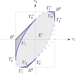
Figure 2. The image of $\boldsymbol{\tau_{2}}$ is the gray subset of the hexagon with continuous and dashed sides. In the light gray region $E^{-}$ the map $\boldsymbol{\tau_{2}}$ is $1$–to–$1,$ while in the medium gray region $U_{0}\cup U_{1}\cup U_{2}$ the map $\boldsymbol{\tau_{2}}$ is $2$–to–$1.$ The vertices $R^{i}$ and the continuous part of the border of the hexagon and the blue ellipse $E$ are in the image, and there $\boldsymbol{\tau_{2}}$ is $1$–to–$1.$ The points $T_{i}^{\pm}$ and the dashed part of the border of the hexagon and $E$ do not belong to Im($\boldsymbol{\tau_{2}}$).

Im$(\boldsymbol{\tau_{2}})$ is a subset of a convex polytope $P_{2}$, the hexagon defined by:

(4) $$\left\{\begin{array}[]{l}-d_{10}\leq\tau_{1}\leq d_{10}\\ -d_{20}\leq\tau_{2}\leq d_{20}\\ -d_{21}\leq\tau_{2}-\tau_{1}\leq d_{21}\end{array}\right..$$

There exists a unique ellipse $E$ tangent to each facet of $P_{2}$ (at the six points $T_{i}^{\pm},\ i=0,1,2$), the one defined by

(5) $$a(\boldsymbol{\tau})=\|\tau_{2}\mathbf{d_{10}}-\tau_{1}\mathbf{d_{20}}\|^{2}-\|\mathbf{d_{10}}\wedge\mathbf{d_{20}}\|^{2}=0.$$

We name $E^{-}$ and $E^{+}$ the interior and the exterior region of the ellipse, respectively, while $U_{0},U_{1},U_{2}$ are the three disjoint connected components of $\mathring{P_{2}}\setminus(E^{-}\cup E)$. Using this notation, we have

(6) $$\mbox{Im}(\boldsymbol{\tau_{2}})=E^{-}\cup\bar{U}_{0}\cup\bar{U}_{1}\cup\bar{U}_{2}\setminus\{T_{0}^{\pm},T_{1}^{\pm},T_{2}^{\pm}\}$$

and in particular

(7) $$|\boldsymbol{\tau_{2}}^{-1}(\boldsymbol{\tau})|=\begin{cases}2&\text{if }\ \boldsymbol{\tau}\in U_{0}\cup U_{1}\cup U_{2},\\ 1&\text{if }\ \boldsymbol{\tau}\in\mbox{Im}(\boldsymbol{\tau_{2}})\setminus U_{0}\cup U_{1}\cup U_{2}.\end{cases}$$

Furthermore, it holds:

1. $\boldsymbol{\tau}\in E$ if, and only if, the hyperbola branches

   (8) $$A_{i}(\boldsymbol{\tau})=\{\mathbf{x}\ |\ d_{i}(\mathbf{x})-d_{0}(\mathbf{x})=\tau_{i}\},i=1,2,$$

   have one of the two asymptotic lines parallel each other. This means that there could exist a source at a great distance from the microphones, in comparison to $d_{10}$ and $d_{20}$. If $\boldsymbol{\tau}\in E\cap\mbox{Im}(\boldsymbol{\tau_{2}})$ the hyperbola branches meet at a point at finite distance, too, which corresponds to another admissible source position.

2. $\boldsymbol{\tau}\in E^{-}$ if, and only if, the hyperbola branches $A-1(\boldsymbol{\tau})$ and $A_{2}(\boldsymbol{\tau})$ meet at one simple point and so, for a given $\boldsymbol{\tau}$, there exists a unique source position $\mathbf{x}$. In this case the localization is still possible even in a noisy scenario, but we lose in precision and stability as $\boldsymbol{\tau}$ gets close to $E$.

3. $\boldsymbol{\tau}\in U_{0}\cup U_{1}\cup U_{2}$ if, and only if, the previous hyperbola branches intersect at two distinct points, which means that for a given $\boldsymbol{\tau}$ there are two admissible source positions. The two solutions overlap if $\boldsymbol{\tau}\in\partial P_{2}$, which corresponds to the tangential intersection of the branches.

Each preimage $\mathbf{x}$ of a given $\boldsymbol{\tau}\in\mbox{Im}(\boldsymbol{\tau_{2}})$, i.e. the admissible source locations, is given in a very compact form through the formalism of exterior algebra over $3$–dimensional Minkowski space–time as:

(9) $$\mathbf{x}(\boldsymbol{\tau})=\mathbf{L_{0}}(\boldsymbol{\tau})+\lambda(\boldsymbol{\tau})\ast((\tau_{2}\mathbf{d_{10}}-\tau_{1}\mathbf{d_{20}})\wedge\mathbf{e_{3}}),$$

where $\lambda$ is one of the real negative solutions of a certain quadratic equation (see [12] for the full details). Roughly speaking, in the physical plane there are two different regions: the preimage of the interior of the ellipse $E^{-}$, where the TDOA map is $1$–to–$1$ and the source localization is possible, and the preimage of the three disjoint regions $U_{i},\ i=0,1,2$, where the map is $2$–to–$1$ and there is no way to uniquely locate the source. By definition, the region of transition is exactly the bifurcation curve $\tilde{E}$, that can be characterized as the inverse image of the ellipse $E$. In the remaining part of this section we recall the main results on the behavior of $\boldsymbol{\tau_{2}}$ in the physical plane. In Figure 3 we give two examples of bifurcation curve and the relative sets.

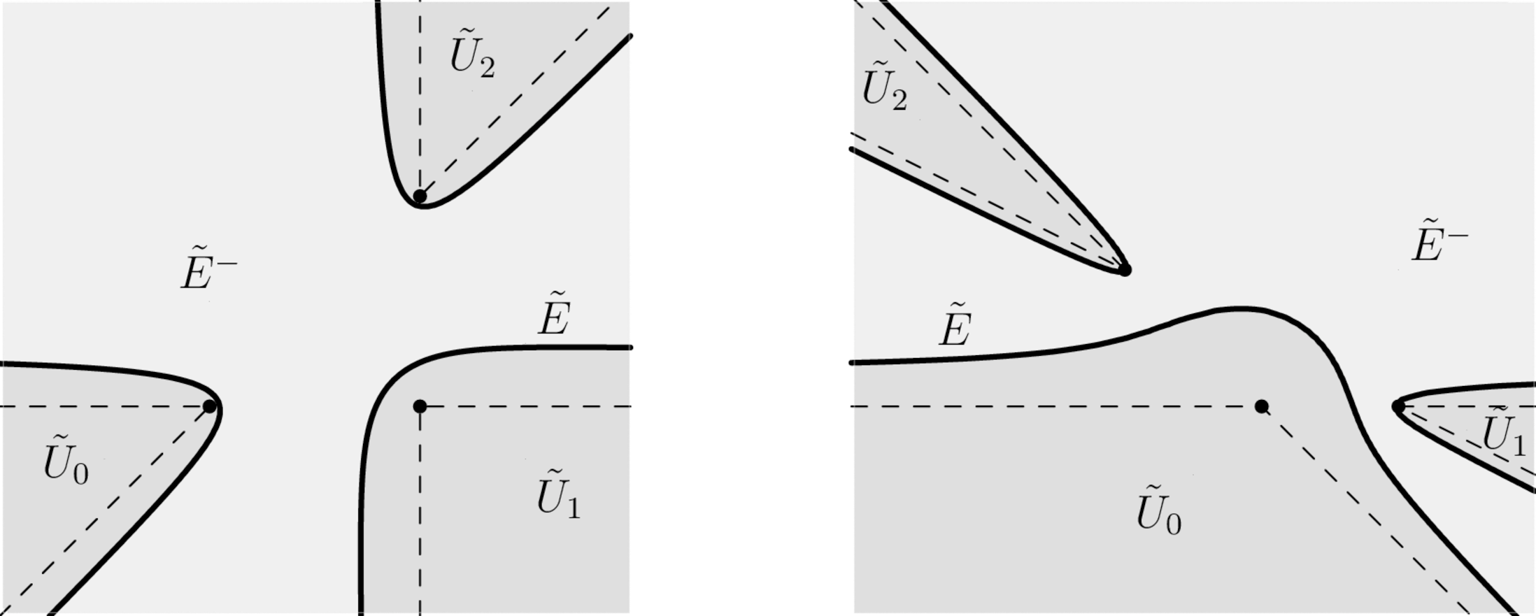
Figure 3. Two examples of the different localization regions and the curve $\tilde{E}$ in the $x$–plane. The microphones are the marked points $\mathbf{m_{0}}=(0,0),\ \mathbf{m_{1}}=(2,0),$ and either $\mathbf{m_{2}}=(2,2)$ on the left, or $\mathbf{m_{2}}=(-2,2)$ on the right. Each curve $\tilde{E}$ separates the light gray region $\tilde{E}^{-}$, where the map $\boldsymbol{\tau_{2}}$ is 1–1 and it is possible to locate the source, and the medium gray region $\tilde{U}_{0}\cup\tilde{U}_{1}\cup\tilde{U}_{2}$, where $\boldsymbol{\tau_{2}}$ is 2–1 and the localization is not unique. On the dashed lines the localization is possible but unstable.

1. As we said above, $\tilde{E}=\boldsymbol{\tau_{2}}^{-1}(E)$. If $\boldsymbol{\tau}\in E$, $\lambda(\boldsymbol{\tau})$ is a rational function and (9) becomes a rational parametrization of $\tilde{E}$. In [12] it has been proved that $\tilde{E}$ is a rational algebraic curve of degree $5$, singular on the complex plane but smooth on the real one.

2. The real part of $\tilde{E}$ consists of three disjoint and unbounded arcs, one for each arc of $E$ contained in $\mbox{Im}(\boldsymbol{\tau_{2}}).$ In particular, when $\boldsymbol{\tau}$ gets close to one point among the $T_{i}^{\pm}$’s in $E\cap C$, the point $\mathbf{x}$ on $\tilde{E}$ goes to infinity. This fact and the invariance of (9) under the reflection $\boldsymbol{\tau}\rightarrow-\boldsymbol{\tau}$ imply that the quintic $\tilde{E}$ has three real ideal points (the ones of the lines $r_{0},r_{1},r_{2},$), while the remaining two ones are the (complex) preimages of the (complex) ideal points of $E.$ Finally, the points $\mathbf{m_{0}},\mathbf{m_{1}},\mathbf{m_{2}}$ do not belong to $\tilde{E},$ because their images via $\boldsymbol{\tau_{2}}$ are not on $E.$

3. Let $\tilde{U}_{i}$ be the inverse image of $U_{i}$ via $\boldsymbol{\tau_{2}},$ for $i=0,1,2,$ and $\tilde{E}^{-}$ be the inverse image of $E^{-}.$ Then, $\tilde{E}^{-},\tilde{U}_{0},\tilde{U}_{1},\tilde{U}_{2}$ are open subsets of the $x$–plane, which are separated by the three arcs of $\tilde{E}$. On $\tilde{E}^{-}$ the TDOA map is $1$–to–$1$, while it is $2$–to–$1$ on each $\tilde{U}_{i},\ i=0,1,2$. Moreover, the dashed half–lines in Figure 3 outgoing from the receivers divide each $\tilde{U}_{i}$ into two connected components and $\boldsymbol{\tau_{2}}$ is $1$–to–$1$ on each of them.

4. The source localization is possible if $\boldsymbol{\tau}\in E^{-}$ and consequently $\mathbf{x}\in\tilde{E}^{-}$. Otherwise, assume $\boldsymbol{\tau}\in U_{i}$, then there are two admissible sources in the two disjoint components of $\tilde{U}_{i}$. As $\boldsymbol{\tau}$ gets close to $E$, then one of its inverse images gets close to a point on $\tilde{E}$, while the other one goes to infinity. Conversely, if $\boldsymbol{\tau}$ gets close to $\partial P_{2}$, the inverse images of $\boldsymbol{\tau}$ come close to each other and get close to a point on one of the dashed half–lines. As we said before, in a realistic noisy scenario, we have poor localization in the region close to $\tilde{E}$.

3. The algebraic equation of $\tilde{E}$ and its asymptotic lines

In this section, we use the formalism of exterior algebra over the Euclidean plane, and we refer to Appendix A of [12]) for a brief introduction and summary on the subject and for the notation. However, from the general results, it follows that

$$\ast(\mathbb{u}\wedge\mathbb{v})=\det\left(\begin{array}[]{cc}u_{1}&v_{1}\\ u_{2}&v_{2}\end{array}\right)$$

where $\mathbb{u}=u_{1}\mathbb{e}_{1}+u_{2}\mathbb{e}_{2},\mathbb{v}=v_{1}\mathbb{e}_{1}+v_{2}\mathbb{e}_{2}$ and $(\mathbb{e}_{1},\mathbb{e}_{2})$ is an orthonormal basis of $\mathbb{R}^{2}.$

Definition 3.1.

Let us define:

1. $\mathbf{D_{0}}(\mathbf{x})=d_{0}(\mathbf{x})\mathbf{d_{12}},\quad\mathbf{D_{1}}(\mathbf{x})=d_{1}(\mathbf{x})\mathbf{d_{20}},\quad\mathbf{D_{2}}(\mathbf{x})=d_{2}(\mathbf{x})\mathbf{d_{01}};$

2. $D_{i}(\mathbf{x})=\|\mathbf{D_{i}(\mathbf{x})}\|\quad and\quad\displaystyle{p_{i}(\mathbf{x})=\frac{\mathbf{D_{i}}(\mathbf{x})\cdot\mathbf{d_{0}}(\mathbf{x})}{d_{i}(\mathbf{x})}},\ i=0,1,2;$

3. $W=\ast(\mathbf{d_{10}}\wedge\mathbf{d_{20}})$;

4. $Q(\mathbf{x})=D_{0}(\mathbf{x})^{2}+D_{1}(\mathbf{x})^{2}+D_{2}(\mathbf{x})^{2}-W^{2};$

5. $P_{ij}(\mathbf{x})=\mathbf{D_{i}}(\mathbf{x})\!\cdot\!\mathbf{D_{j}}(\mathbf{x})\quad and\quad\displaystyle{p_{ij}=\frac{P_{ij}(\mathbf{x})}{d_{i}(\mathbf{x})d_{j}(\mathbf{x})}},\quad i,j=0,1,2.$

Theorem 3.2.

An algebraic equation for the quintic curve $\tilde{E}$ is $F(\mathbf{x})=0$, where:

(10) $$\begin{array}[]{l}F(\mathbf{x})=Q(\mathbf{x})^{4}-8\,Q(\mathbf{x})^{2}(P_{01}(\mathbf{x})^{2}+P_{12}(\mathbf{x})^{2}+P_{20}(\mathbf{x})^{2})\,+\\ 64\,Q(\mathbf{x})P_{01}(\mathbf{x})P_{12}(\mathbf{x})P_{20}(\mathbf{x})+16\,(P_{01}(\mathbf{x})^{4}+P_{12}(\mathbf{x})^{4}+P_{20}(\mathbf{x})^{4})\\ -32\,(P_{01}(\mathbf{x})^{2}P_{12}(\mathbf{x})^{2}+P_{12}(\mathbf{x})^{2}P_{20}(\mathbf{x})^{2}+P_{20}(\mathbf{x})^{2}P_{01}(\mathbf{x})^{2}).\end{array}$$

The polynomial $F(\mathbf{x})$ is invariant under permutation of the points $\mathbf{m_{0}},$ $\mathbf{m_{1}},\mathbf{m_{2}}$. Expanding (10) with respect to $d_{0}(\mathbf{x})$, we have:

(11) $$\begin{array}[]{ll}F(\mathbf{x})\!=\!\!\!\!&((W^{2}+2(d_{20}^{2}\,p_{2}(\mathbf{x})-d_{01}^{2}\,p_{1}(\mathbf{x})))^{2}+16\,p_{12}^{2}\,p_{1}(\mathbf{x})\,p_{2}(\mathbf{x}))^{2}+\\ &8\,d_{0}(\mathbf{x})^{2}(-W^{4}\,p_{12}\,(-8\,d_{01}^{2}d_{20}^{2}+p_{01}\,p_{20}+2W^{2})+\\ &2W^{2}((W^{2}+2\,p_{12}^{2})(W^{2}+3\,p_{12}^{2})(p_{2}(\mathbf{x})-p_{1}(\mathbf{x}))+\\ &3\,p_{12}\,(2\,d_{01}^{2}\,d_{20}^{2}+W^{2})(d_{20}^{2}\,p_{2}(\mathbf{x})-d_{01}^{2}\,p_{1}(\mathbf{x}))+\\ &2\,p_{12}^{2}\,(p_{01}\,d_{20}^{2}\,p_{2}(\mathbf{x})-p_{20}\,d_{01}^{2}\,p_{1}(\mathbf{x})))+\\ &4(d_{20}^{2}\,p_{2}(\mathbf{x})-d_{01}^{2}\,p_{1}(\mathbf{x}))^{2}(2(d_{01}^{2}+d_{20}^{2})W^{2}+7\,p_{01}\,p_{12}\,p_{20})-\\ &8(d_{20}^{2}\,p_{2}(\mathbf{x})-d_{01}^{2}\,p_{1}(\mathbf{x}))(W^{2}p_{12}^{2}\,(p_{2}(\mathbf{x})-p_{1}(\mathbf{x}))+\\ &(W^{2}+4p_{12}^{2})(p_{01}^{2}\,p_{2}(\mathbf{x})-p_{20}^{2}\,p_{1}(\mathbf{x})))-\\ &16\,p_{12}\,p_{1}(\mathbf{x})p_{2}(\mathbf{x})(2W^{2}d_{01}^{2}d_{20}^{2}+p_{12}^{2}\,p_{20}\,p_{01})+\\ &2\,d_{0}(\mathbf{x})^{2}(p_{12}(d_{01}^{2}+d_{20}^{2})(4\,d_{01}^{2}d_{20}^{2}W^{2}+\\ &p_{12}^{2}(2\,p_{20}\,p_{01}-p_{12}(d_{01}^{2}+d_{20}^{2})))+d_{01}^{2}d_{20}^{2}(4d_{01}^{4}d_{20}^{4}-7W^{4}))-\\ &8Wd_{01}^{2}d_{12}^{2}d_{20}^{2}\!\ast\!\!(\mathbf{d_{01}}\wedge\mathbf{d_{0}}(\mathbf{x}))\!\ast\!\!(\mathbf{d_{12}}\wedge\mathbf{d_{0}}(\mathbf{x}))\!\ast\!\!(\mathbf{d_{20}}\wedge\mathbf{d_{0}}(\mathbf{x}))).\end{array}$$

Proof.

The bifurcation curve $\tilde{E}$ is the preimage of the ellipse $E$, therefore we obtain a Cartesian equation of $\tilde{E}$ by substituting $(\tau_{1},\tau_{2})=(\tau_{10}(\mathbf{x}),\tau_{20}(\mathbf{x}))$ in (5):

(12) $$\|(d_{2}(\mathbf{x})-d_{0}(\mathbf{x}))\mathbf{d_{10}}-(d_{1}(\mathbf{x})-d_{0}(\mathbf{x}))\mathbf{d_{20}}\|^{2}=(\ast(\mathbf{d_{10}}\wedge\mathbf{d_{20}}))^{2}.$$

Using Definitions 3.1, we have the more symmetric form

(13) $$\|\mathbf{D_{0}}(\mathbf{x})+\mathbf{D_{1}}(\mathbf{x})+\mathbf{D_{2}}(\mathbf{x})\|^{2}=W^{2}$$

and, after expanding the left hand side,

(14) $$\begin{array}[]{l}D_{0}(\mathbf{x})^{2}+D_{1}(\mathbf{x})^{2}+D_{2}(\mathbf{x})^{2}+\\ 2\,(\mathbf{D_{0}}(\mathbf{x})\!\cdot\!\mathbf{D_{1}}(\mathbf{x})+\mathbf{D_{1}}(\mathbf{x})\!\cdot\!\mathbf{D_{2}}(\mathbf{x})+\mathbf{D_{2}}(\mathbf{x})\!\cdot\!\mathbf{D_{0}}(\mathbf{x}))=W^{2}.\end{array}$$

Of course, this is not an algebraic equation with respect to $x,y$. In order to obtain one, we use again Definitions 3.1 and we rewrite equation (14) as

(15) $$Q(\mathbf{x})+2P_{12}(\mathbf{x})=-2\,(P_{01}(\mathbf{x})+P_{20}(\mathbf{x})).$$

By squaring both sides and reordering, we obtain:

(16) $$\begin{array}[]{l}Q(\mathbf{x})^{2}-4(P_{01}(\mathbf{x})^{2}-P_{12}(\mathbf{x})^{2}+P_{20}(\mathbf{x})^{2})=\\ -4\,Q(\mathbf{x})\,P_{12}(\mathbf{x})+8\,P_{01}(\mathbf{x})\,P_{20}(\mathbf{x})\end{array}$$

Again, the right side of the last equation is not a polynomial, but squaring once we get the algebraic equation:

(17) $$\begin{array}[]{l}(Q(\mathbf{x})^{2}-4(P_{01}(\mathbf{x})^{2}-P_{12}(\mathbf{x})^{2}+P_{20}(\mathbf{x})^{2}))^{2}=16\,Q(\mathbf{x})^{2}\,P_{12}(\mathbf{x})^{2}\\ -64\,Q(\mathbf{x})\,P_{01}(\mathbf{x})\,P_{12}(\mathbf{x})\,P_{20}(\mathbf{x})+64\,P_{01}(\mathbf{x})^{2}\,P_{20}(\mathbf{x})^{2},\end{array}$$

that coincides with equation $F(\mathbf{x})=0$. It is straightforward to verify that (10) is invariant with respect to permutations of the points $\mathbf{m_{0}},\mathbf{m_{1}},\mathbf{m_{2}}$.

The degree of polynomial (10) with respect to $(x,y)$ is 8 at the most. By calculating the Taylor expansion (11) of (10) centered at the point $\mathbf{m_{0}}$, we show that $F(\mathbf{x})$ has degree $5$ and this completes the proof (the verification of expansion (11) is a simple matter of computation). ∎

Remark 3.3.

If the receivers are not collinear, we have that $F(\mathbf{m_{0}})=F(\mathbf{m_{1}})=F(\mathbf{m_{2}})=W^{8}>0$. Therefore $\mathbf{x}\in\tilde{E}^{-}$ if, and only if, $F(\mathbf{x})<0$ and $\mathbf{x}\in\tilde{E}^{+}$ if, and only if, $F(\mathbf{x})>0$.

As an example, we provide the Cartesian equations of the two bifurcation curves of Fig. 3. The bifurcation curve on the left has equation

$$\begin{split}\tilde{E}:&-4x^{4}y+4x^{3}y^{2}-4x^{2}y^{3}+4xy^{4}+2x^{4}+20x^{3}y-16x^{2}y^{2}+4xy^{3}+\\ &-6y^{4}-10x^{3}-38x^{2}y+30xy^{2}+2y^{3}+18x^{2}+28xy-22y^{2}+\\ &-12x-4y+1=0\end{split}$$

while the one of the right has equation

$$\begin{split}\tilde{E}:&-20x^{4}y-60x^{3}y^{2}-60x^{2}y^{3}-60xy^{4}-40y^{5}+10x^{4}+68x^{3}y+\\ &+80x^{2}y^{2}+84xy^{3}+82y^{4}-34x^{3}-58x^{2}y-10xy^{2}-50y^{3}+30x^{2}+\\ &+4xy+22y^{2}-4x-4y+1=0.\end{split}$$

Using polynomial (11) we can compute an algebraic expression for the real asymptotic lines of $\tilde{E}$. We refer to Appendix B of [12] for an introduction to projective geometry. As a preliminary, we prove the following Lemma.

Lemma 3.4.

$\displaystyle{W=\frac{\ast(\mathbf{d_{12}}\wedge\mathbf{d_{0}}(\mathbf{x}))+\ast(\mathbf{d_{20}}\wedge\mathbf{d_{1}}(\mathbf{x}))+\ast(\mathbf{d_{01}}\wedge\mathbf{d_{2}}(\mathbf{x}))}{2}}$.

Proof.

We use the following identities

(18) $$\mathbf{d_{01}}+\mathbf{d_{12}}+\mathbf{d_{20}}=0,\qquad\mathbf{d_{ij}}=\mathbf{d_{j}}(\mathbf{x})-\mathbf{d_{i}}(\mathbf{x}),\qquad i,j=0,1,2.$$

We have

(19) $$\begin{array}[]{ll}\mathbf{d_{10}}\wedge\mathbf{d_{20}}&=(\mathbf{d_{0}}(\mathbf{x})-\mathbf{d_{1}}(\mathbf{x}))\wedge\mathbf{d_{20}}=\\ &=\mathbf{d_{0}}(\mathbf{x})\wedge(\mathbf{d_{21}}+\mathbf{d_{10}})-\mathbf{d_{1}}(\mathbf{x})\wedge\mathbf{d_{20}}=\\ &=\mathbf{d_{12}}\wedge\mathbf{d_{0}}(\mathbf{x})+\mathbf{d_{20}}\wedge\mathbf{d_{1}}(\mathbf{x})+(\mathbf{d_{2}}(\mathbf{x})+\mathbf{d_{20}})\wedge\mathbf{d_{10}}=\\ &=\mathbf{d_{12}}\wedge\mathbf{d_{0}}(\mathbf{x})+\mathbf{d_{20}}\wedge\mathbf{d_{1}}(\mathbf{x})+\mathbf{d_{01}}\wedge\mathbf{d_{2}}(\mathbf{x})-\mathbf{d_{10}}\wedge\mathbf{d_{20}}.\end{array}$$

The Lemma follows from Definition 3.1 and the last identity. ∎

Definition 3.5.

Let $\mathbb{A}^{2}$ be the affine plane, and let $\mathbb{P}^{2}$ be the projective plane obtained by joining the ideal line $\ell$ to $\mathbb{A}^{2}.$ Let $C$ be an algebraic curve in the affine plane $\mathbb{A}^{2}$. The ideal points of $C$ are the intersection points of $C$ and the ideal line $\ell.$ An asymptotic line of $C$ is a line in $\mathbb{A}^{2}$ tangent to $C$ at one of its smooth ideal points.

Let $f(x,y)=0$ be the Cartesian equation of a degree $d$ algebraic curve $C$ in $\mathbb{A}^{2}.$ We can write it as

$$f(x,y)=f_{d}(x,y)+f_{d-1}(x,y)+\dots+f_{1}(x,y)+f_{0}$$

where $f_{i}(x,y)$ is homogeneous of degree $i.$ We embed $\mathbb{A}^{2}$ into $\mathbb{P}^{2}$ by setting $x=X/U,y=Y/U,$ and $\ell:U=0$ is the ideal line. The curve $C\subset\mathbb{P}^{2}$ is then defined by

$$F(X,Y,U)=f_{d}(X,Y)+f_{d-1}(X,Y)U+\dots+f_{1}(X,Y)U^{d-1}+f_{0}U^{d}.$$

The ideal points are the solutions, in the sense of projective geometry, of $U=f_{d}(X,Y)=0.$ Let $[a:b:0]$ be a smooth ideal point of $C.$ So, the line $r:-bx+ay+c=0$ is an asymptotic line for $C$ if $[a:b:0]$ is a solution of $F(X,Y,U)=-bX+aY+cU=0$ of multiplicity at least two.

Theorem 3.6.

The bifurcation curve $\tilde{E}$ has three real ideal points $[x_{1}-x_{2}:y_{1}-y_{2}:0],[x_{2}-x_{0}:y_{2}-y_{0}:0],[x_{0}-x_{1}:y_{0}-y_{1}:0]$ and two complex ones $[1:i:0],[1:-i:0].$
The three real asymptotic lines of $\tilde{E}$ have Cartesian equation

(20) $$\begin{array}[]{l}L_{0}:\ 4\ast(\mathbf{d_{12}}\wedge\mathbf{d_{0}}(\mathbf{x}))-3W=0,\\ L_{1}:\ 4\ast(\mathbf{d_{20}}\wedge\mathbf{d_{1}}(\mathbf{x}))-3W=0,\\ L_{2}:\ 4\ast(\mathbf{d_{01}}\wedge\mathbf{d_{2}}(\mathbf{x}))-3W=0.\end{array}$$

Finally, we have $L_{0}\cap L_{1}\cap L_{2}=\emptyset.$

Proof.

The homogeneous degree–$5$ part of polynomial (11) is

(21) $$-64Wd_{01}^{2}d_{12}^{2}d_{20}^{2}\,d_{0}(\mathbf{x})^{2}\ast(\mathbf{d_{12}}\wedge\mathbf{d_{0}}(\mathbf{x}))\ast(\mathbf{d_{20}}\wedge\mathbf{d_{0}}(\mathbf{x}))\ast(\mathbf{d_{01}}\wedge\mathbf{d_{0}}(\mathbf{x}))$$

and so it is straightforward to check that the five ideal points of the statement are its roots, and they all are smooth for $\tilde{E}.$ By using a package for algebraic computations, it is easy to prove that $L_{i}$ meets $C$ at the corresponding ideal point with multiplicity $2,$ and this proves that the line $L_{i}$ is asymptotic to $C.$

The last statement follows from Lemma 3.4. In fact, if we sum the three polynomials (20) defining the asymptotic lines, we obtain

(22) $$\begin{array}[]{l}4\ast(\mathbf{d_{12}}\wedge\mathbf{d_{0}}(\mathbf{x})+\mathbf{d_{20}}\wedge\mathbf{d_{1}}(\mathbf{x})+\mathbf{d_{01}}\wedge\mathbf{d_{2}}(\mathbf{x}))-9W=-W.\end{array}$$

Thus, the three lines do not have a common intersection point: in fact, if there exists a common point $\mathbf{x}_{0},$ its coordinates satisfy also the sum of the three equations of the asymptotic lines. Such a sum is $W=0,$ and so $\mathbf{x}_{0}$ does not exist. ∎

As $\tilde{E}$ is a quintic curve, each line $L_{i}$ intersects $\tilde{E}$ at either $1$ or $3$ real points. Hence, also if it is not evident from Fig. 3, the unbounded arcs of $\tilde{E}$ definitely belong to different half–planes with respect to its asymptotic lines.

4. Conclusion

In this paper, we recall the state of the art on the localization of sources in a plane from the TDOAs for the case of $3$ receivers in the same plane. Then, we focus on a problem still open in the literature: the computation of the Cartesian algebraic equation of the bifurcation curve $\tilde{E},$ that is to say, of the curve in the plane of source and receivers whose points are sources for which the hyperbola branches (8) have an asymptotic line parallel each other. The knowledge of such an equation allows us to easily solve the problem of finding points in the plane which are close or belong to such a curve $\tilde{E}.$ The importance of computing the equation of $\tilde{E}$ stems from the fact that at its points, every localization algorithm has a poor accuracy. The computation of the Cartesian equation of the bifurcation curve rests on two steps: first, by squaring a non–polynomial equation for $\tilde{E},$ we compute a polynomial; then, by using a Taylor expansion, we get the explicit degree five equation. From such equation, it is possible to compute the real asymptotic lines of $\tilde{E}.$ Notice that it is not possible to compute such lines from the parametric equation of $\tilde{E}.$

In [12] as well as in the present paper, we completed the geometric study of the noiseless model of localization, encoded in the TDOA map $\boldsymbol{\tau}_{2},$ for the case of $3$ receivers in a plane. In a manuscript in preparation, we will conduct a similar study for a real scenario. Other then the deterministic case, the needed techniques come from information geometry [3] and statistics with algebraic tools [13, 22], and from numerical analysis. Moreover, still in preparation, we are studying the geometry of the noiseless model in the case of $4$ or more receivers in a plane.

References

- [1] J. Abel and J. Chauffe. Existence and uniqueness of GPS solutions. IEEE Transactions on Aerospace and Electronic Systems, 27:952–956, November 1991.
- [2] J. Abel and J. Smith. The spherical interpolation method for closed-form passive source localization using range difference measurements. In Acoustics, Speech, and Signal Processing, IEEE International Conference on ICASSP ’87., volume 12, pages 471 – 474, apr 1987.
- [3] S. Amari and H. Nagaoka. Methods of Information Geometry. American Mathematical Society, 2000.
- [4] J.L. Awange and J. Shan. Algebraic Solution of GPS Pseudo-Ranging Equations. GPS Solutions, 5(4):20–32, 2002.
- [5] S. Bancroft. An Algebraic Solution of the GPS Equations. IEEE Transactions on Aerospace Electronic Systems, 21:56–59, January 1985.
- [6] A. Beck, P. Stoica, and Jian Li. Exact and approximate solutions of source localization problems. Signal Processing, IEEE Transactions on, 56(5):1770 –1778, May 2008.
- [7] P. Bestagini, M. Compagnoni, F. Antonacci, A. Sarti, and S. Tubaro. Tdoa-based acoustic source localization in the space–range reference frame. Multidimensional Systems and Signal Processing, 2013.
- [8] C.B. Boyer. A History of Mathematics. New York: Wiley, 1989.
- [9] J. Chauffe and J. Abel. On the exact solution of the pseudorange equations. IEEE Transactions on Aerospace and Electronic Systems, 30:1021–1030, October 1994.
- [10] B. Coll, J. Ferrando, and J. Morales-Lladosa. Positioning systems in minkowski space-time: from emission to inertial coordinates. Classical Quantum Gravity, 27:065013, 2010.
- [11] B. Coll, J. Ferrando, and J. Morales-Lladosa. Positioning systems in minkowski space-time: Bifurcation problem and observational data. Phys. Rev. D, 86:084036, Oct 2012.
- [12] Marco Compagnoni, Roberto Notari, Fabio Antonacci, and Augusto Sarti. A comprehensive analysis of the geometry of tdoa maps in localization problems. Inverse Problems, 30(3):035004, 2014.
- [13] J. Draisma, E. Horobet, G. Ottaviani, B. Sturmfels, and R.R. Thomas. The Euclidean distance degree of an algebraic variety. 2013.
- [14] I.A. Getting. The Global Positioning System. IEEE Spectrum, SPEC-30:36–47, December 1993.
- [15] M. Gillette and H. Silverman. A linear closed-form algorithm for source localization from time-differences of arrival. IEEE Signal Processing Letters, 15:1–4, 2008.
- [16] E.W. Grafarend and J. Shan. GPS Solutions: Closed Forms, Critical and Special Configurations of P4P. GPS Solutions, 5(3):29–41, 2002.
- [17] J. Hoshen. The GPS Equations and the Problem of Apollonius. IEEE Transactions on Aerospace and Electronic Systems, 32(3):1116–1124, July 1996.
- [18] Y. Huang and J. Benesty. Audio Signal Processing for Next Generation Multimedia Communication Systems. Kluwer Academic Publishers, 2004.
- [19] Y. Huang, J. Benesty, and G.W. Elko. Passive acoustic source localization for video camera steering. In Acoustics, Speech, and Signal Processing, 2000. ICASSP ’00. Proceedings. 2000 IEEE International Conference on, volume 2, pages II909 –II912 vol.2, 2000.
- [20] Y. Huang, J. Benesty, G.W. Elko, and R.M. Mersereati. Real-time passive source localization: a practical linear-correction least-squares approach. Speech and Audio Processing, IEEE Transactions on, 9(8):943 –956, November 2001.
- [21] Y. Huang, J. Benesty, and G.Elko. Source Localization, chapter 9, pages 229–253. Kluwer Academic Publishers, 2004.
- [22] K. Kobayashi and H.P. Wynn. Computational algebraic methods in efficient estimation. 2013.
- [23] L.O. Kraus. A direct solution to GPS-type navigation equations. IEEE Transactions on Aerospace and Electronic Systems, AES-23(2):223–232, March 1987.
- [24] J. Leva. An alternative closed form solution to the GPS pseudorange equation. In Proceedings of the Institute of Navigation National Technical Meeting, pages 269–271, Anaheim, CA, January 1995.
- [25] H. Schau and A. Robinson. Passive source localization employing intersecting spherical surfaces from time-of-arrival differences. Acoustics, Speech and Signal Processing, IEEE Transactions on, 35(8):1223 – 1225, August 1987.
- [26] R.O. Schmidt. A new approach to geometry of range difference location. Aerospace and Electronic Systems, IEEE Transactions on, AES-8(6):821 –835, Nov. 1972.
- [27] G.M. Siouris. Aerospace Avionics Systems. Academic Press, San Diego, 1993.
- [28] J. Smith and J. Abel. The spherical interpolation method of source localization. Oceanic Engineering, IEEE Journal of, 12(1):246 – 252, jan 1987.
- [29] J. Smith and J. S. Abel. Closed-form least-squares source location estimation from range-difference measurements. IEEE Trans. Acoust., Speech, Signal Processing, ASSP-35:1661–1669, 1987.
- [30] S.J. Spencer. The two-dimensional source location problem for time differences of arrival at minimal element monitoring arrays. J. Acoust. Soc. Am., 121(6):3579–3594, June 2007.
- [31] S.J. Spencer. Closed–form analytical solutions of the time difference of arrival source location problem for minimal element monitoring arrays. J. Acoust. Soc. Am., 127(5):2943–2954, May 2010.