Sparsity-aware sphere decoding: Algorithms and complexity analysis

Abstract

Integer least-squares problems, concerned with solving a system of equations where the components of the unknown vector are integer-valued, arise in a wide range of applications. In many scenarios the unknown vector is sparse, i.e., a large fraction of its entries are zero. Examples include applications in wireless communications, digital fingerprinting, and array-comparative genomic hybridization systems. Sphere decoding, commonly used for solving integer least-squares problems, can utilize the knowledge about sparsity of the unknown vector to perform computationally efficient search for the solution. In this paper, we formulate and analyze the sparsity-aware sphere decoding algorithm that imposes $\ell_{0}$-norm constraint on the admissible solution. Analytical expressions for the expected complexity of the algorithm for alphabets typical of sparse channel estimation and source allocation applications are derived and validated through extensive simulations. The results demonstrate superior performance and speed of sparsity-aware sphere decoder compared to the conventional sparsity-unaware sphere decoding algorithm. Moreover, variance of the complexity of the sparsity-aware sphere decoding algorithm for binary alphabets is derived. The search space of the proposed algorithm can be further reduced by imposing lower bounds on the value of the objective function. The algorithm is modified to allow for such a lower bounding technique and simulations illustrating efficacy of the method are presented. Performance of the algorithm is demonstrated in an application to sparse channel estimation, where it is shown that sparsity-aware sphere decoder performs close to theoretical lower limits.

I Introduction

Given a matrix ${\bf H}\in\mathbb{R}^{n\times m}$ and a vector ${\mathbf{y}}\in\mathbb{R}^{n\times 1}$, the integer least-squares (ILS) problem is concerned with finding an $m$-dimensional vector ${\bf x}^{\star}$ comprising integer entries such that

$${\bf x}^{\star}~{}=~{}\arg\underset{{\bf x}\in\mathbb{Z}^{m}}{\min}~{}~{}\|{\mathbf{y}}-{\mathbf{H}}{\mathbf{x}}\|_{2}^{2},$$ (1)

where $\mathbb{Z}^{m}$ denotes the $m$-dimensional integer lattice. In many applications, the unknown vector ${\mathbf{x}}$ belongs to a finite $m$-dimensional subset $\mathcal{D}_{L}^{m}$ of the infinite lattice $\mathbb{Z}^{m}$ such that $\mathcal{D}_{L}^{m}$ has $L$ elements per dimension, i.e., each component of the unknown vector ${\mathbf{x}}$ can take one of $L$ possible discrete values from the set $\mathcal{D}_{L}\subset\mathbb{Z}$. In multi-antenna communication systems, for instance, ${\mathbf{x}}\in\mathcal{D}_{L}^{m}$ is the transmitted symbol while the received signal ${\mathbf{y}}={\bf H}{\mathbf{x}}+\boldsymbol{\nu}$ is perturbed by the additive noise $\boldsymbol{\nu}$ (hence, $\boldsymbol{\nu}$ renders the system of equations ${\mathbf{y}}\approx{\bf H}{\mathbf{x}}$ inconsistent). Note that the symbols in $\mathcal{D}_{L}^{m}$ form an $m$-dimensional rectangular lattice and, therefore, ${\bf Hx}$ belongs to an $n$-dimensional lattice skewed in the direction of the eigenvectors of ${\bf H}$. An integer least-squares problem can be interpreted as the search for the nearest point in a given lattice, commonly referred to as the closest lattice point problem [1]. Geometric interpretation of the integer least-squares problem as the closest lattice point search is illustrated in Fig. 1(a).

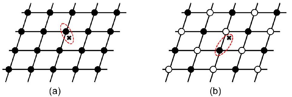
Figure 1: Illustration of the search for the closest lattice point. The black dots in both subfigures denote lattice points ${\mathbf{H}}{\mathbf{x}}$. ${\bf\times}$ marks the observed vector ${\mathbf{y}}$. Subfigure (a) illustrates the scenario where all lattice points are admissible while (b) illustrates the scenario where the unknown vector is sparse and thus not all lattice point can be the solution.

Integer least-squares problems with sparse solutions arise in a broad range of applications including multi-user detection in wireless communication systems [2], sparse array processing [3], collusion-resistant digital fingerprinting [4], and array-comparative genomic hybridization microarrays [5]. Formally, a sparse integer least-squares problem can be stated as the cardinality constrained optimization

$$\min_{{\mathbf{x}}\in\mathcal{D}_{L}^{m}}~{}~{}~{}~{}~{}~{}\|{\mathbf{y}}-{\mathbf{H}}{\mathbf{x}}\|_{2}^{2}$$ (2)

$$\mbox{subject to }~{}~{}~{}\|{\mathbf{x}}\|_{0}~{}\leq~{}l,$$

where $\|\cdot\|_{0}$ denotes the $\ell_{0}$ norm of its argument and $l$ is an upper bound on the number of non-zero entries of ${\mathbf{x}}$. In this paper, we restrict our attention to the case where $n\geq m$ (all of the aforementioned applications fall in this category). Note that (2) can be interpreted as a search for the lattice point ${\mathbf{H}}{\mathbf{x}}$ closest to the given point ${\bf y}$ in a sparse lattice, where the sparsity constraint is explicitly stated as $\{{\mathbf{x}}\in\mathcal{D}_{L}^{m}~{}|~{}\|{\mathbf{x}}\|_{0}\leq l\}$. Search over a sparse lattice is illustrated in Fig. 1(b).

Finding the exact solution to (2) is computationally intensive (in fact, the closest lattice point problem is known to be NP hard [6]). The sphere decoding algorithm, developed by Fincke and Pohst [7], efficiently solves the ILS problem and provides optimal solution in a broad range of scenarios [8, 9, 10]. In particular, it was shown in [9, 10] that if the sphere radius is chosen using the statistics of $\boldsymbol{\nu}={\mathbf{y}}-{\mathbf{H}}{\mathbf{x}}$, then the sphere decoding algorithm has an expected complexity that is practically feasible over a wide range of problem parameters.

Recently, several variants of sphere decoder that exploit information about sparsity of the unknown vector were proposed [3], [11], [2]. In [3], a modified sphere decoding algorithm with the $\ell_{0}$-norm constraint relaxed to an $\ell_{1}$-norm regularizer was proposed. This scheme is only applicable to non-negative alphabets, in which case $\|{\mathbf{x}}\|_{1}$ can be decomposed into the sum of the components of ${\mathbf{x}}$. In [11], a generalized sphere decoding approach imposing an $\ell_{1}$ constraint on the solution was adopted for sparse integer least-square problems over binary alphabets. That work examines the case where $n<m$ and essentially considers compressed sensing scenario. An $\ell_{0}$-norm regularized sphere decoder has been proposed and studied in [2], where the regularizing parameter $\lambda$ was chosen to be a function of the prior probabilities of the activity of independent users in a multiuser detection environment. In contrast, sphere decoder in the present manuscript directly imposes the $\ell_{0}$-norm constraint on the unknown vector, i.e., we perform no relaxation or regularization of the distance metric. Note that the closest point search in a sparse lattice has previously been studied in [12] but sparsity there stems from the fact that not all lattice points are valid codewords of linear block codes. In [13], a sparse integer least-squares problem arising in the context of spatial modulation was studied for the special case of symbol vectors with single non-zero entry; the method there does not rely on the branch-and-bound search typically used by sphere decoding. Note that none of the previous works on characterizing complexity of sphere decoder (see, e.g., [14], [15], [16] and the references therein) considered sparse integer least-squares problems except for [17], where the worst-case complexity of sphere decoder in spatial modulation systems of [13] was studied. Finally, we should also point out a considerable amount of related research on compressed sensing, where one is interested in the recovery of an inherently sparse signal by using potentially far fewer measurements than what is typically needed for a signal which is not sparse [18]-[24].

The paper is organized as follows. In Section II, we review the sphere decoding algorithm and formalize its sparsity-aware variant. Following the analysis framework in [9, 10], in Section III we derive the expected complexity of the sparsity-aware sphere decoder for binary and ternary alphabets commonly encountered in various applications. The derived analytical expressions are validated via simulations. Section IV presents an expression for the variance of the complexity of the proposed algorithm for binary alphabets. In Section V, the algorithm is modified by introducing an additional mechanism for pruning nodes in the search tree, leading to a significant reduction of the number of points traversed and the overall computational complexity. In Section VI, performance of the algorithm is demonstrated in an application to sparse channel estimation. The paper is summarized in Section VII.

II Algorithms

In this section, we first briefly review the classical sphere decoding algorithm and then discuss its modification that accounts for sparsity of the unknown vector.

II-A Sphere decoding algorithm

To find the closest point in an $m$-dimensional lattice, sphere decoder performs the search within an $m$-dimensional sphere of radius $d$ centered at the given point ${\mathbf{y}}\in\mathbb{R}^{n}$. In particular, to solve (1), the sphere decoding algorithm searches over ${\mathbf{x}}$ such that $d^{2}\geq\|{\bf y}-{\bf Hx}\|^{2}$. The search procedure is reminiscent of the branch-and-bound optimization [25]. In a pre-processing step, one typically starts with the $QR$-decomposition of ${\mathbf{H}}$,

$${\mathbf{H}} = [{\mathbf{Q}}_{1}~{}~{}{\mathbf{Q}}_{2}]\left[\begin{array}[]{c}{\mathbf{R}}\\ {\bf 0}_{(n-m\times m)}\end{array}\right],$$ (5)

where ${\mathbf{R}}$ is the upper-triangular matrix and ${\mathbf{Q}}_{1}$ and ${\mathbf{Q}}_{2}$ are composed of the first $m$ and the last $n-m$ orthonormal columns of ${\mathbf{Q}}$, respectively. Therefore, we can rewrite the sphere constraint $d^{2}\geq\|{\bf y}-{\bf Hx}\|^{2}$ as

$$d^{2}-\|{\mathbf{Q}}_{2}^{*}{\bf y}\|^{2} \geq \|{\bf z}-{\mathbf{R}}{\bf x}\|_{2}^{2},$$ (6)

where ${\bf z}={\mathbf{Q}}_{1}^{*}{\bf y}$. Now, (6) can be expanded to

$$d^{2}-\|{\mathbf{Q}}_{2}^{*}{\bf y}\|^{2}\geq(z_{m}-R_{m,m}x_{m})^{2}+(z_{m-1}-R_{m-1,m}x_{m}-R_{m-1,m-1}x_{m-1})^{2}+\cdots$$ (7)

where $x_{i}$ and $z_{i}$ are the $i^{th}$ components of ${\mathbf{x}}$ and ${\mathbf{z}}$, respectively, and $R_{i,j}$ is the $(i,j)^{th}$ entry of ${\mathbf{R}}$. Note that the first term on the right-hand side (RHS) of (7) depends only on $x_{m}$, the second term on $\{x_{m},x_{m-1}\}$, and so on. A necessary (but not sufficient) condition for ${\bf Hx}$ to lie inside the sphere is $d^{2}-\|{\mathbf{Q}}_{2}^{*}{\bf y}\|^{2}\geq(z_{m}-R_{m,m}x_{m})^{2}$. For every $x_{m}$ satisfying this condition, a stronger necessary condition can be found by considering the first two terms on the RHS of (7) and imposing a condition that $x_{m-1}$ should satisfy to lie within the sphere. One can proceed in a similar fashion to determine conditions for $x_{m-2},\ldots,x_{1}$, thereby determining all the lattice points that satisfy $d^{2}\geq\|{\bf y}-{\bf Hx}\|^{2}_{2}$. If no point is found within the sphere, its radius is increased and the search is repeated. If multiple points satisfying the constraint are found, then the one yielding the smallest value of the objective function is declared the solution. Clearly, the choice of the radius is of critical importance for facilitating a computationally efficient search. If $d$ is too large, the search complexity may become infeasible, while if $d$ is too small, no lattice point will be found within the sphere. To this end, $d$ can be chosen according to the statistics of $\boldsymbol{\nu}={\mathbf{y}}-{\mathbf{H}}{\mathbf{x}}$, hence providing probabilistic guarantee that a point is found inside the sphere [9].

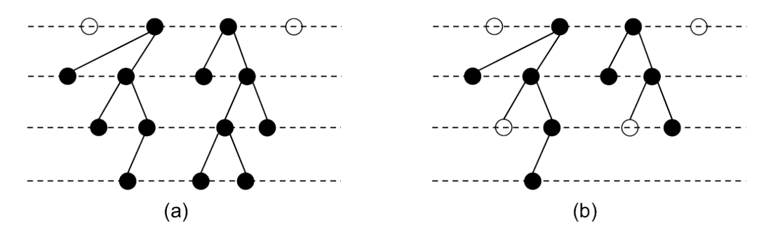
Figure 2: An illustration of the depth-first tree search of the sphere decoding algorithm when (a) the unknown vector is non-sparse and (b) the unknown vector is sparse.

The sphere decoding algorithm can be interpreted as a search on a tree, as illustrated in Fig. 2(a). The nodes at the $k^{th}$ tree level represent $k$-dimensional points $[x_{m-k+1}~{}x_{m-k+2}~{}\ldots x_{m}]^{T}$ . The algorithm uses aforementioned constraints to prune nodes from the tree, keeping only those that belong to the $k$-dimensional sphere of radius $d$. Many variants of the basic sphere decoding have been developed [26], [27] - [28].

II-B Sparsity-aware sphere decoding

In scenarios where the unknown vector ${\mathbf{x}}$ is known to be sparse, imposing $\ell_{0}$-norm constraint on ${\bf x}$ improves the speed of the search since the necessary conditions that the components of ${\bf x}$ must satisfy become more restrictive. Clearly, not all lattice points within the search sphere satisfy the sparsity constraint and thus fewer points need to be examined in each step of the sparsity-aware sphere decoding algorithm. We impose sparsity constraint on the components of ${\bf x}$ at each node of the search tree traversed by the algorithm. Note that the number of non-zero symbols along the path from the root node to a given node is a measure of the sparseness of the $k$-dimensional point associated with that node. Suppose that a node at the $k^{th}$ level of the tree satisfies the sphere constraint. Sparsity constraint implies that, in addition to the node being inside the sphere, the number of non-zero symbols along the path leading to the node must not exceed an upper bound $l$. Hence, knowledge of sparsity allows us to impose more strict conditions on the potential solutions to the integer least-squares problems, and the number of nodes that the algorithm prunes is greater than that in the absence of sparsity (or in the absence of the knowledge about sparsity).

TABLE I: Sparsity-aware Sphere Decoding Algorithm

Input: $Q=[Q_{1}~{}~{}Q_{2}],~{}R,y,~{}z=Q_{1}^{*}y,$ sphere radius $d$,

sparsity constraint $l$.

1. Initialize $k\leftarrow m$, $d_{m}^{2}\leftarrow d^{2}-\|Q_{2}^{*}y\|^{2}$,

$z_{m|m+1}\leftarrow z_{m}$, $l_{m}\leftarrow 0$ .

2. Update Interval    $UB(x_{k})\leftarrow\left\lfloor(d_{k}+z_{k|k+1})/R_{k,k}\right\rfloor$,

$LB(x_{k})\leftarrow\left\lceil(-d_{k}+z_{k|k+1})/R_{k,k}\right\rceil$, $x_{k}\leftarrow LB(x_{k})-1$.

3. Update $x_{k}$    $x_{k}\leftarrow x_{k}+1$. If $x_{k}\leq UB(x_{k}),$

go to 4; else go to 5.

4. Check Sparsity     If $l_{k}+\mathcal{I}_{\{x_{k}\neq 0\}}\leq l,~{}$

$l_{k}\leftarrow l_{k}+\mathcal{I}_{\{x_{k}\neq 0\}}$, and go to 6; else go to 3.

5. Increase $k$    $k\leftarrow k+1$. If $k=m+1,$ stop;

else, $l_{k}\leftarrow l_{k}-\mathcal{I}_{\{x_{k}\neq 0\}}$ and go to 3.

6. Decrease $k$ If $k=1,$ go to 7; else $k\leftarrow k-1$,

$z_{k|k+1}\leftarrow z_{k}-\sum_{j=k+1}^{m}R_{k,j}x_{j},$

$d_{k}^{2}\leftarrow d_{k+1}^{2}$ $-(z_{k+1|k+2}-R_{k+1,k+1}x_{k+1})^{2},$ and go to 2.

7. Solution found   Save $x$ and its distance from $y$,

$d_{m}^{2}-d_{1}^{2}+(z_{1}-R_{1,1}~{}x_{1})^{2},~{}l_{k}\leftarrow l_{k}-\mathcal{I}_{\{x_{k}\neq 0\}}$

and go to 3.

Table I formalizes the sparsity-aware sphere decoding algorithm with $\ell_{0}$-norm constraint imposed on the solution. Note that, in the pseudo-code, variable $l_{k}$ denotes the number of non-zero symbols selected in the first $k-1$ levels. This variable is used to impose the sparsity constraint in Step 4 of the algorithm (calculating $l_{k}$ and imposing the sparsity constraint requires only a minor increase in the number of computations per node). Whenever the algorithm backtracks up a level in the tree, the value of $l_{k}$ is adjusted to reflect sparseness of the current node (as indicated in Steps 5 and 7 of the algorithm). The depth-first tree search of the sparsity-aware sphere decoding algorithm is illustrated in Figure 2(b), where fewer points survive pruning than in Figure 2(a).

Remark 1: The algorithm in Table I relies on the original Fincke-Pohst strategy for conducting the tree search [7]. There exist more efficient implementations such as the so-called Schnorr-Euchner variant of sphere decoding where the search in each dimension $k$ starts from the middle of the feasible interval for $x_{k}$ and proceeds to explore remaining points in the interval in a “zig-zag” fashion (for details see, e.g., [1]). For computational benefits, one should combine such a search strategy with radius update, i.e., as soon as a valid point ${\mathbf{x}}_{in}$ inside the sphere is found, the algorithm should be restarted with the radius equal to $\|{\mathbf{y}}-{\mathbf{H}}{\mathbf{x}}_{in}\|$. The expected complexity results derived in Section III are exact for the Fincke-Pohst search strategy and can be viewed as an upper bound on the expected complexity of the Schnorr-Euchner scheme with radius update.

Remark 2: The pseudo-code of the algorithm shown in Table I assumes an alphabet having unit spacing, which can be generalized in a straightforward manner. For non-negative alphabets, the algorithm can be further improved by imposing the condition that if a node at a given level violates the sparsity constraint, then all the remaining nodes at that level will also violate the constraint. Details are omitted for brevity.

We should also point out that, in addition to helping improve computational complexity, utilizing knowledge about sparseness of the unknown vector also improves accuracy of the algorithm. To illustrate this, in Figure 3 we compare the error rate (i.e., the average fraction of the incorrectly inferred components of ${\mathbf{x}}$) performance of sparsity-aware sphere decoder with that of the classical (sparsity-unaware) sphere decoding algorithm. In this figure, the error rate is plotted as a function of the sparsity ratio $l/m$. We use a sparse binary alphabet, and simulate a system with $m=n=20$ at SNR = 10 dB. The classical sphere decoder is unaware of the sparseness of the unknown vector (i.e., it essentially assumes $l=20$). It is shown in the figure that the sparsity-aware sphere decoding algorithm performs exceptionally well compared to classical sphere decoder for low values of $l$. As expected, the performance gap between the two decoders diminishes if the unknown vector is less sparse. For a comparison, Figure 3 also shows performance of the method where the relaxed version of the integer least-squares problem is solved via orthogonal matching pursuit (OMP) and the result is then rounded to the nearest integer in the symbol space. It is worthwhile mentioning that the OMP method is sub-optimal since there are no guarantees that it will find the closest lattice point. Therefore, its performance (as well as performances of other sub-optimal schemes such as LASSO) is generally inferior to that of sparsity-aware sphere decoder, as illustrated in Figure 3 - Figure 3. Figure 3 shows the error rates as the function of the relative sparsity level $l/m$ for $m=n=20$. Figure 3 illustrates the same but for $m=n=40$. Performances of the considered algorithms in Figure 3 and Figure 3 exhibit the same trends – i.e., the performance gap between sparsity-aware SD and classical SD widens as the sparsity ratio $l/m$ reduces. Figure 4 shows the error rate performance of sparsity-aware and classical sphere decoder, along with OMP, as a function of SNR, while $l$ is fixed at $5$. In this figure too, sparsity-aware sphere decoder is seen to dramatically outperform its classical counterpart as well as OMP.

III Expected Complexity of Sparsity-Aware Sphere Decoding

As elaborated in [9], computational complexity of the sphere decoding algorithm depends on the effective size of the search tree, i.e., the number of nodes in the tree visited by the algorithm during the search for the optimal solution to the integer least-squares problem. If both ${\mathbf{H}}$ and $\boldsymbol{\nu}$ are random variables, so is the number of tree nodes visited by the algorithm. Therefore, it is meaningful to treat the complexity as a random variable and characterize it via a distribution or its moments. This motivates the study of the expected complexity of the sparsity-aware sphere decoding algorithm presented next.

Assume that $\boldsymbol{\nu}={\mathbf{y}}-{\bf H}{\mathbf{x}}$ (the perturbation noise) consists of independent, identically distributed entries having Gaussian distribution $\mathcal{N}(0,\sigma^{2})$. Clearly, $\frac{1}{\sigma^{2}}\|\boldsymbol{\nu}\|^{2}$ is a random variable following $\chi_{n}^{2}$ distribution. As argued in [9], if the radius of the search sphere is chosen as $d^{2}=\alpha n\sigma^{2}$, where $\alpha$ is such that $\gamma(\frac{\alpha n}{2},\frac{n}{2})=1-\epsilon$ for small $\epsilon>0$, then with high probability the sphere decoding algorithm will visit at least one lattice point. Moreover, with such a choice of the radius, the probability that an arbitrary lattice point ${\mathbf{H}}{\bf x}_{a}$ belongs to a

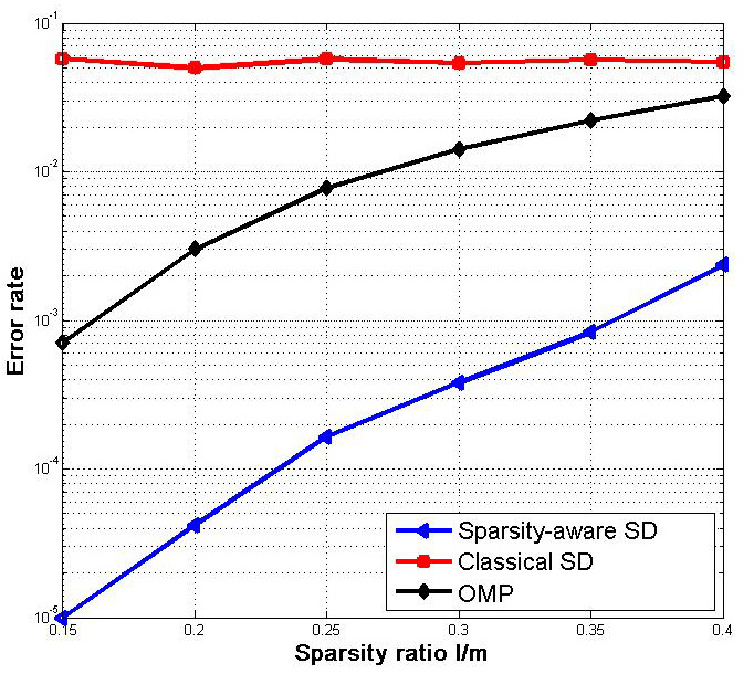
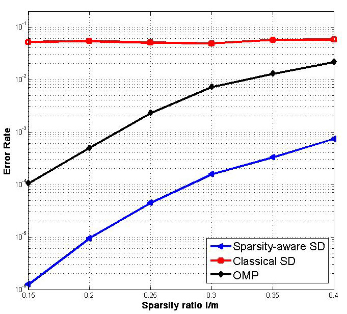
Figure 3: Error rate of sparsity-aware SD and classical SD as a function of the sparsity ratio $l/m$ in subfigure (a) and (b) for binary $\{0,1\}$ alphabet at SNR = $10$ dB. For (a), $m=n=20$ and for (b), $m=n=40$. Performance of the suboptimal OMP algorithm, where the integer constraint on the entries of ${\mathbf{x}}$ is relaxed and the solution to the relaxed problem is rounded off to nearest integer in the alphabet, is also shown.

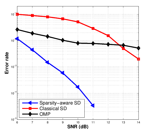
Figure 4: Error rate of sparsity-aware SD and classical SD as a function of SNR for binary $\{0,1\}$ alphabet with $m=n=20$ and $l=5$. Performance of the suboptimal OMP algorithm, where the integer constraint on the entries of ${\mathbf{x}}$ is relaxed and the solution to the relaxed problem is rounded off to nearest integer in the alphabet, is also shown.

sphere $\mathcal{S}_{d}$ of radius $d$ centered at $\bf y$ is

$$\mathcal{P}({\bf x}_{a}\in\mathcal{S}_{d}) = \mathcal{P}\left(\|{\mathbf{y}}-{\mathbf{H}}{\mathbf{x}}_{a}\|_{2}^{2}\leq d^{2}\right)$$ (8)

$$= \gamma\left(\frac{d^{2}}{2(\sigma^{2}+\|{\bf x}_{a}-{\bf x}_{t}\|^{2})},\frac{n}{2}\right),$$

where ${\bf x}_{t}$ denotes the true value of the unknown vector $\bf x$.

Let $N_{k}$ be the random variable denoting the number of points in the tree visited by the sparsity-aware sphere decoding algorithm searching for an $l$-sparse solution to (2). It is easy to see that

$$\mathbb{E}\left[N_{k}|~{}{\mathbf{x}}_{t},d^{2}\right]=\sum_{\eta}\sum_{\begin{subarray}{c}{\mathbf{x}}_{a}^{k}~{}:~{}{\mathbf{x}}_{a}^{k}\in\mathcal{D}_{L}^{k},\\ \|{\mathbf{x}}_{t}^{k}-{\mathbf{x}}_{a}^{k}\|^{2}=\eta\\ \|{\mathbf{x}}_{a}^{k}\|_{0}\leq l\end{subarray}}\gamma\Big{(}\frac{d^{2}}{2(\sigma^{2}+\eta)},\frac{n-m+k}{2}\Big{)},$$ (9)

where ${\mathbf{x}}^{k}$ denotes the vector consisting of the last $k$-entries of ${\mathbf{x}}$, i.e., ${\mathbf{x}}^{k}=[x_{m-k+1}~{}\cdots~{}x_{m}]$. Note that the inner sum in (9) is only over those ${\mathbf{x}}_{a}^{k}$ that satisfy the sparsity constraint. Therefore, the expected number of points visited by our sparsity-aware sphere decoder, averaged over all permissible ${\bf x}_{t}$, is given by

$$\mathbb{E}\left[N_{k}|~{}d^{2}\right] = \mathbb{E}\left[\mathbb{E}\left[N_{k}|~{}{\mathbf{x}}_{t},d^{2}\right]\right]$$ (10)

$$= \sum_{\begin{subarray}{c}{\mathbf{x}}_{t}^{k}:{\mathbf{x}}_{t}^{k}\in\mathcal{D}_{L}^{k}\\ \|{\mathbf{x}}_{t}^{k}\|_{0}\leq l\end{subarray}}~{}p({\mathbf{x}}_{t}^{k})~{}\mathbb{E}\left[N_{k}|~{}{\mathbf{x}}_{t},d^{2}\right]$$ (11)

where the outer expectation in (10) is evaluated with respect to ${\mathbf{x}}_{t}$, and $p({\mathbf{x}}_{t}^{k})$ in (11) denotes the probability that ${\mathbf{x}}_{t}^{k}$ is the true value of ${\mathbf{x}}^{k}$. Note that without the sparsity constraint on ${\mathbf{x}}_{t}$, it would hold that $p({\mathbf{x}}_{t}^{k})=1/L^{k},~{}\forall k$, where $L$ denotes the alphabet size. However, due to the sparsity constraint, $p({\mathbf{x}}_{t}^{k})$ is not uniform. As an illustration, consider a simple example of the $2$-dimensional $1$-sparse set on the binary $\{0,1\}$ alphabet comprising of vectors $\{(0,0),(0,1),(1,0)\}$. If all $x_{t}$ are equally likely, it is easy to see that the probability of ${\mathbf{x}}_{t}^{1}$ is given by $p({\mathbf{x}}_{t}^{1}=1)=1/3=1-p({\mathbf{x}}_{t}^{1}=0)$. For a general $l$-sparse $m$-dimensional constellation, the probability distribution $p({\mathbf{x}}_{t}^{k})$ can be obtained by enumerating all $k$-dimensional vectors in the set for $k=1,2,\cdots,m$.

Having determined expected number of lattice points visited by the sparsity-aware sphere decoding algorithm, the average complexity can be expressed as

$$C(m,d^{2})=\sum\limits_{k=1}^{m}~{}f(k)~{}\mathbb{E}\left[N_{k}|~{}d^{2}\right],$$ (12)

where $f(k)$ denotes the number of operations performed by the algorithm in the $k^{th}$ dimension.

The main challenge in evaluating (9) is to find an efficient enumeration of the symbol space, i.e., to determine the number of $l$-sparse vectors ${\bf x}_{a}^{k}$ such that $\|{\bf x}_{t}^{k}-{\bf x}_{a}^{k}\|^{2}=\eta$ for a given ${\mathbf{x}}_{t}^{k}$. While this enumeration appears to be difficult in general, it can be found in a closed form for some of the most commonly encountered alphabets in sparse integer least square problems: the binary $\{0,1\}$ alphabet (relevant to applications in [4], [29] and [30]) and the ternary $\{-1,0,1\}$ alphabet (relevant to application in [5]). In the rest of this section, we provide closed form expressions of the expected complexity of sparsity-aware sphere decoder for these alphabets.

III-A Binary Alphabet {0,1}

Recall that computing (9) requires enumeration of the sparse symbol space, i.e., counting $l$-sparse vectors ${\mathbf{x}}_{a}^{k}\in\mathcal{D}_{L}^{k}$ satisfying $\|{\mathbf{x}}_{a}^{k}-{\mathbf{x}}_{t}^{k}\|^{2}=\eta$ for a given $l$-sparse vector ${\mathbf{x}}_{t}^{k}\in\mathcal{D}_{L}^{k}$ and $\eta$. Note that, for the binary alphabet, condition $\|{\mathbf{x}}_{t}^{k}-{\mathbf{x}}_{a}^{k}\|_{2}^{2}=\eta$ is equivalent to $\|{\mathbf{x}}_{t}^{k}-{\mathbf{x}}_{a}^{k}\|_{0}=\eta$. Let $\|{\mathbf{x}}_{t}^{k}\|_{0}=k_{1}$, and denote the $i^{th}$ entry of ${\mathbf{x}}^{k}$ as ${\mathbf{x}}^{k}(i),~{}i=1,\cdots,k$. Furthermore, let $\|{\mathbf{x}}_{t}\|_{0}=k_{3}$.

Lemma 1: Given $k_{1}=\|{\mathbf{x}}_{t}^{k}\|_{0}$ and $\eta$, the number of $k$-dimensional lattice points ${\mathbf{x}}_{a}^{k}$ with $\|{\mathbf{x}}_{a}^{k}\|_{0}=k_{2}$ such that $\|x_{a}^{k}-x_{t}^{k}\|^{2}=\eta$ is given by

$$g(k_{1},k_{2},k,\eta)=\binom{k_{1}}{p}\binom{k-k_{1}}{q},$$ (13)

where

$$p=\frac{1}{2}(\eta-(k_{2}-k_{1})),~{}q=k-k_{2}-p, k_{1}<k_{2}$$ if

$$q=\frac{1}{2}(\eta-(k_{1}-k_{2})),~{}p=k_{2}-q, k_{1}\geq k_{2}$$ if

Proof:

See Appendix A. ∎

Note that for a given ${\mathbf{x}}_{t}^{k}$ and $k_{2}$, the possible values of $\eta$ belong to the set $\mathcal{S}=\{|k_{1}-k_{2}|,|k_{1}-k_{2}|+2,\cdots,\min{(k_{1}+k_{2},k)}\}$. Then, (9) can be written as

$$\mathbb{E}[N_{k}|~{}{\mathbf{x}}_{t},d^{2}]=\sum_{k_{2}=0}^{\min(k,l)}\sum\limits_{\eta\in\mathcal{S}}\gamma\left(\frac{d^{2}}{2(\sigma^{2}+\eta)},\frac{n-m+k}{2}\right)g(k_{1},k_{2},k,\eta).$$ (14)

Finally, outer expectation in (10) is enumerated as follows. Total number of sparse binary vectors ${\mathbf{x}}_{t}^{k}$ for a given $k$ can be parameterized by $k_{1}$ and $k_{3}$. For ${\mathbf{x}}_{t}$ to be $l$-sparse, $0\leq k_{3}\leq l$ and for each $k_{3}$, it should hold that $(k_{3}-(m-k))_{+}\leq k_{1}\leq\min{(k,k_{3})}$. The number of ${\mathbf{x}}_{t}$ vectors for each pair of values of $k_{3}$ and $k_{1}$ is then given by $\binom{k}{k_{1}}\binom{m-k}{k_{3}-k_{1}}$. Therefore, the total number of all possible $l$-sparse vectors ${\mathbf{x}}_{t}$ is given as $N=\sum\limits_{k_{3},k_{1}}\binom{k}{k_{1}}\binom{m-k}{k_{3}-k_{1}}$ and (11) can be written in terms of $k_{3}$ and $k_{1}$ as

$$\mathbb{E}\left[N_{k}|~{}d^{2}\right]=\frac{1}{N}\sum\limits_{k_{3},k_{1}}~{}\binom{k}{k_{1}}\binom{m-k}{k_{3}-k_{1}}~{}\mathbb{E}\left[N_{k}|~{}{\mathbf{x}}_{t},d^{2}\right]$$ (15)

where the summations are evaluated over respective ranges as described above.

Theorem 1: The expected number of tree points examined by the sparsity-aware sphere decoding algorithm while solving (2) over a binary alphabet is

$$\mathbb{E}\left[N_{k}|d^{2}\right]=\frac{1}{N}\sum\limits_{k_{3}=0}^{l}~{}~{}~{}\sum\limits_{k_{1}={(k_{3}-(m-k))}_{+}}^{\min{(k,k_{3})}}\binom{k}{k_{1}}\binom{m-k}{k_{3}-k_{1}}\Big{[}\sum_{k_{2}=0}^{\min(k,l)}\sum\limits_{\eta\in\mathcal{S}}\gamma\left(\frac{d^{2}}{2(\sigma^{2}+\eta)},\frac{n-m+k}{2}\right)g(k_{1},k_{2},k,\eta)\Big{]},$$ (16)

where $d$ denotes the search radius and $g(k_{1},k_{2},k,\eta)$ is defined in (13).

Proof:

The proof follows from (9) and Lemma 1.

∎

Remark: Note that (16) has important implications on the worst-case complexity of the sparsity-aware sphere decoding algorithm. Assume, for the sake of argument, that the radius $d$ of the sphere is sufficiently large to cover the entire lattice. In the absence of the radius constraint, pruning of the search tree happens only when the sparsity constraint is violated, and hence (14) reduces to

$$\mathbb{E}\left[N_{k}|~{}{\mathbf{x}}_{t},d^{2}\right] = \sum_{k_{2}=0}^{\min(k,\ell)}\sum\limits_{\eta\in\mathcal{S}}g(k_{1},k_{2},k,\eta)$$ (17)

$$= \sum_{k_{2}=0}^{\min(k,\ell)}\binom{k}{k_{2}}.$$

Expression (17) essentially represents the worst-case scenario where a brute-force search over all $l$-sparse signals is required, leading to a complexity exponential in $k$. For $k<l$, this is clearly the case. For $k\geq l$, the partial sum of binomial coefficients in (17) cannot be computed in a closed form but its various approximations and bounds exists in literature. For example, it has been shown in [31] that the partial sum of binomial coefficients in (17) grows exponentially in $k$ if $l=k/a$ for a constant $a\geq 2$. A corollary to this result states that if $a$ is an unbounded, monotonically increasing function, the sum in (17) does not grow exponentially in $k$. Therefore, unless the fraction of the non-zero components of ${\mathbf{x}}$ becomes vanishingly small as the dimension of ${\mathbf{x}}$ grows, the worst-case complexity of the sparsity-aware sphere decoding algorithm is exponential in $m$ (the length of ${\mathbf{x}}$).

Also note that if ${\mathbf{x}}_{t}$ is $l$-sparse but the sparsity constraint is not invoked at the decoder (i.e., the decoder is sparsity-unaware), then (14) is reduced to

$$\mathbb{E}\left[N_{k}|~{}{\mathbf{x}}_{t},d^{2}\right]=\sum_{k_{2}=0}^{k}\sum\limits_{\eta\in\mathcal{S}}\gamma\left(\frac{d^{2}}{2(\sigma^{2}+\eta)},\frac{n-m+k}{2}\right)g(k_{1},k_{2},k,\eta).$$ (18)

Clearly, (18) is an upper bound for (14), and hence exploiting sparsity information enables reduction of the expected complexity.

III-B Ternary Alphabet {-1,0,1}

Define the support sets $S_{j}({\mathbf{x}}_{t}^{k})$ of ${\mathbf{x}}_{t}^{k}$ for $j\in\{-1,0,1\}$ and let $a=|S_{1}({\mathbf{x}}_{t}^{k})|$. Unlike the binary case, here we evaluate (9) by reversing the order of summation, i.e., by enumerating all possible $l$-sparse vectors ${\mathbf{x}}_{a}^{k}$ and then summing over all $\eta$ such that $\|{\mathbf{x}}_{t}^{k}-{\mathbf{x}}_{a}^{k}\|_{2}^{2}=\eta$. To this end, let us introduce

$$p_{i,j}=\sum\limits_{r\in S_{i}({\mathbf{x}}_{t}^{k})}\mathcal{I}_{\{{\mathbf{x}}_{a}^{k}(r)=j\}},\;\;\;i,j\in\{-1,0,1\}.$$ (19)

In words, $p_{i,j}$ denote the number of symbols $j$ in ${\mathbf{x}}_{a}^{k}$ in the positions where ${\mathbf{x}}_{t}^{k}$ has symbol $i$. It is easy to see that $\sum_{i}\sum_{j}p_{i,j}=k$ and, furthermore,

$$\sum\limits_{j}p_{i,j}=\begin{cases}a,&i=1\\ k_{1}-a,&i=-1\\ k-k_{1},&i=0.\end{cases}$$ (20)

where $k_{1}=\|{\mathbf{x}}_{t}^{k}\|_{0}$. Given $p_{i,j}$, $\eta$ can be written as

$$\eta = \sum\limits_{i,j}p_{i,j}|i-j|^{2}.$$ (21)

Lemma 2: Given $k_{1}=\|{\mathbf{x}}_{t}^{k}\|_{0}$ and $\eta$, the number of $k$-dimensional lattice points ${\mathbf{x}}_{a}^{k}$ with $\|{\mathbf{x}}_{a}^{k}\|_{0}=k_{2}$ such that $\|x_{a}^{k}-x_{t}^{k}\|^{2}=\eta$ is given by

$$g_{1}(k_{1},k_{2},k,p_{ij})=\binom{a}{p_{1,0}}\binom{a-p_{1,0}}{p_{1,-1}}\binom{k_{1}-a}{p_{-1,0}}\binom{k_{1}-a-p_{-1,0}}{p_{-1,1}}\binom{k-k_{1}}{k_{2}-(k_{1}-p_{-1,0}-p_{1,0})}2^{k_{2}-(k_{1}-p_{-1,0}-p_{1,0})},$$ (22)

for $k_{1}\leq k_{2}$ and

$$g_{2}(k_{1},k_{2},k,p_{ij})=\binom{k-k_{1}}{p_{0,1}+p_{0,-1}}\binom{a}{p_{1,-1}}\binom{a-p_{1,-1}}{p_{1,1}}\binom{k_{1}-a}{p_{-1,1}}\binom{k_{1}-a-p_{-1,1}}{k_{2}-(p_{0,1}+p_{0,-1}+p_{1,-1}+p_{1,1}+p_{-1,1})}2^{p_{0,1}+p_{0,-1}},$$ (23)

for $k_{1}>k_{2}$.

Proof:

See Appendix B. ∎

Similar to the binary case, it can be shown that the total number of $l$-sparse vectors ${\mathbf{x}}_{t}$ is given by $\binom{k}{a}\binom{k-a}{k_{1}-a}\binom{m-k}{k_{3}-k_{1}}2^{k_{3}-k_{1}}$, where $k_{3}=\|{\mathbf{x}}_{t}\|_{0}$, $0\leq k_{3}\leq l$, ${(l-(m-k))}_{+}\leq k_{1}\leq\min{(k,k_{3})}$ and $0\leq a\leq k_{1}$. Therefore, (11) can be written in this case as

$$\mathbb{E}[N_{k}~{}|~{}d^{2}]=\frac{1}{N}\sum\limits_{k_{3},k_{1},a}\binom{k}{a}\binom{k-a}{k_{1}-a}\binom{m-k}{k_{3}-k_{1}}2^{k_{3}-k_{1}}~{}\mathbb{E}[N_{k}|~{}{\mathbf{x}}_{t}^{k},d^{2}],$$

where $N$ is the number of all $l$-sparse vectors ${\mathbf{x}}_{t}$, given by $N=\sum\limits_{k_{3},k_{1},a}\binom{k}{a}\binom{k-a}{k_{1}-a}\binom{m-k}{k_{3}-k_{1}}2^{k_{3}-k_{1}}$, and the summations are evaluated over respective ranges as described above.

Theorem 2: The expected number of tree points examined by the sparsity-aware sphere decoding algorithm while solving (2) over a ternary alphabet is

$$\mathbb{E}[N_{k}|~{}d^{2}]=\frac{1}{N}\sum\limits_{k_{3}=0}^{l}~{}~{}\sum\limits_{k_{1}={(l-(m-k))}_{+}}^{\min{(k,k_{3})}}\sum\limits_{a=0}^{k_{1}}\binom{k}{a}\binom{k-a}{k_{1}-a}\binom{m-k}{k_{3}-k_{1}}2^{k_{3}-k_{1}}$$

$$\times\Bigg{[}\sum\limits_{k_{2}=0}^{k_{1}-1}~{}~{}\sum\limits_{p_{i,j}~{}:~{}k_{1}>k_{2}}\gamma\left(\frac{d^{2}}{2(\sigma^{2}+\eta)},\frac{n-m+k}{2}\right)g_{2}(k_{1},k_{2},k,p_{i,j})\Big{.}$$

$$\Big{.}+\sum\limits_{k_{2}=k_{1}}^{\min{(k,l)}}~{}~{}\sum\limits_{p_{i,j}~{}:~{}k_{1}\leq k_{2}}~{}\gamma\left(\frac{d^{2}}{2(\sigma^{2}+\eta)},\frac{n-m+k}{2}\right)g_{1}(k_{1},k_{2},k,p_{i,j})\Bigg{]}$$ (24)

where the value of $\eta$ is given by (21).

Proof:

The proof follows from (9) and Lemma 2.

∎

III-C Results

It is useful to define the complexity exponent, $e_{c}=\log{C(m,d^{2})}/\log{m}$, as a measure of complexity of the algorithm. To validate the derived theoretical expressions for the expected complexity of the sparsity-aware sphere decoding algorithm, we compare them with empirically evaluated complexity exponents. The results are shown in Fig. 5. Here, parameters of the simulated system are $m=n=20$ and $l=5$. The empirical expected complexity is obtained by averaging over $1000$ Monte Carlo runs. As can be seen in in Fig. 5, the theoretical expressions derived in this section exactly match empirical results and are hence corroborated.

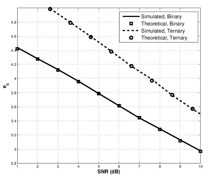
Figure 5: Complexity exponent as a function of SNR for $m=n=20$, $l=5$ for binary $\{0,1\}$ and ternary $\{-1,0,1\}$ alphabets.

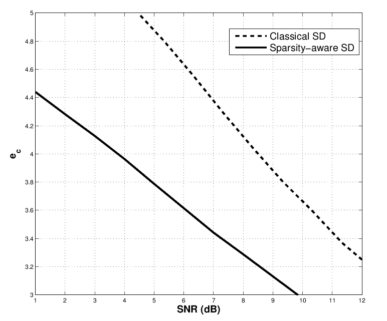
Figure 6: Comparison of the complexity exponent of sparsity-aware sphere decoder and classical (sparsity-unaware) sphere decoder for $m=n=20$, $l=5$ and binary $\{0,1\}$ alphabet.

Fig. 6 compares the complexity exponent of sparsity-aware sphere decoder with that of the classical (sparsity-unaware) sphere decoding algorithm for $m=n=20$, $l=5$ and binary $\{0,1\}$ alphabet. Similar to Fig. 3 and 3, classical sphere decoder assumes the unknown vector to be non-sparse. As can be seen from the plot, the complexity of sparsity-aware sphere decoder is less than that of classical decoder, with the gap being more significant at lower values of signal-to-noise ratios (SNRs) and decreasing as SNR increases. This is expected because, for low SNRs, radius of the sphere is large and the complexity of sparsity-aware sphere decoder approaches that of performing an exhaustive search for the closest point. Since the cardinality of the sparse set in this example is significantly smaller than that of the full lattice, the complexity gap between two algorithms is pronounced. However, for high SNRs, the sphere often contains very few lattice point (occasionally only one), and hence the difference between the complexity exponents of the two algorithms reduces. Also note that the complexity of sparsity-aware sphere decoder decreases with $l$ since the sparsity constraint further reduces the number of points that will be in a sphere of a given radius.

IV Variance Analysis

In this section, we characterize the second-order moment of the complexity of sparsity-aware sphere decoder. The following analysis is restricted to the binary alphabet, but it can be extended to more general alphabets in a relatively straightforward manner. It has been shown in [10] that the variance of the complexity of the sphere decoding algorithm is given by

$$\sigma_{\mbox{\small sparse}}^{2}=\sum\limits_{k=1}^{m}\sum\limits_{l=1}^{m}\left(\mathbb{E}[N_{k}N_{l}]-~{}\mathbb{E}[N_{k}]\mathbb{E}[N_{l}]\right)f(k)f(l),$$ (25)

where $N_{k}$ and $f(k)$ have same meanings as in Section III. Note that (25) applies to the sparsity-aware sphere decoder as well, but $\mathbb{E}[N_{k}]$, $\mathbb{E}[N_{l}]$, and $\mathbb{E}[N_{k}N_{l}]$ differ from those for the classical (sparsity-unaware) algorithm. In Section III, we found an expression for the expected number of points $\mathbb{E}[N_{k}]$ visited by the sparsity-aware sphere decoding algorithm. Therefore, to evaluate (25), what remains to be determined is $\mathbb{E}[N_{k}N_{l}]$, i.e., the correlation between the number of pairs of points of dimensions $k$ and $l$ lying inside a sphere of radius $d$. Let each of these points be $l^{\prime}$-sparse.

Given ${\mathbf{H}}={\mathbf{Q}}{\mathbf{R}}$, and using (6), the correlation between $N_{k}$ and $N_{l}$ can be found as [10]

$$\mathbb{E}[N_{k}N_{l}]=\sum\limits_{{\mathbf{x}}_{B}\in\mathcal{D}_{L}^{k}}~{}\sum\limits_{{\mathbf{x}}_{C}\in\mathcal{D}_{L}^{l}}~{}\mathcal{P}\left(t_{b}\leq d^{2},t_{c}\leq d^{2}\right),$$ (26)

where $t_{b}=\|{\mathbf{z}}^{k}-{\mathbf{R}}(k,k){\mathbf{x}}_{B}\|^{2}$, $t_{c}=\|{\mathbf{z}}^{l}-{\mathbf{R}}(l,l){\mathbf{x}}_{C}\|^{2}$, ${\mathbf{x}}_{B}$ and ${\mathbf{x}}_{C}$ are arbitrary $k$ and $l$ dimensional $l^{\prime}$-sparse vectors having entries from ${\cal D}_{L}$, and ${\mathbf{R}}(p,p)$ is given by the following partition of ${\mathbf{R}}$,

$${\mathbf{R}}=\left[\begin{array}[]{cc}{\mathbf{R}}(m-p,m-p)&{\mathbf{R}}(m-p,p)\\ {\bf 0}_{p\times(m-p)}&{\mathbf{R}}(p,p)\end{array}\right]$$ (29)

for $p=1,\ldots,m$. Let ${\mathbf{x}}_{t}^{k}$ be the $k$-dimensional sub-vector of the true solution, and define ${\mathbf{x}}_{b}={\mathbf{x}}_{t}^{k}-{\mathbf{x}}_{B}$ and ${\mathbf{x}}_{c}={\mathbf{x}}_{t}^{l}-{\mathbf{x}}_{C}$. Depending on whether ${\mathbf{x}}_{b}={\mathbf{x}}_{c}^{k}$ or not, the summand in (26) is given by [10]:

1. If $x_{b}=x_{c}^{k}$,

   $$\mathcal{P}\left(t_{b}\leq d^{2},t_{c}\leq d^{2}\right)=\gamma\left(\frac{d^{2}}{2(\sigma^{2}+\|x_{c}\|^{2})},\frac{l}{2}\right)$$ (30)

2. If $x_{b}\neq x_{c}^{k}$,

   $$\mathcal{P}(t_{b}\leq d^{2},t_{c}\leq d^{2})=\int_{t_{b}=0}^{d^{2}}\int_{t_{c}=0}^{d^{2}}\phi(t_{b},t_{c})dt_{b}dt_{c},$$ (31)

   where $\phi(t_{b},t_{c})$ is given by (32),

   $$\phi(t_{b},t_{c})=\frac{1}{4\pi^{2}}\int_{-\infty}^{\infty}\int_{-\infty}^{\infty}\frac{d\omega_{b}d\omega_{c}e^{-j\omega_{b}t_{b}-j\omega_{c}t_{c}}}{\Delta^{k/2}\left[\left(\frac{a_{bb}}{\Delta}-2j\omega_{c}\right)\left(\frac{a_{cc}}{\Delta}-2j\omega_{b}\right)-\frac{a_{bc}^{2}}{\Delta^{2}}\right]^{k/2}}\frac{\left(1-2j\omega_{c}(\sigma^{2}+\|x_{c}^{k}\|^{2})\right)^{k/2}}{\left(1-2j\omega_{c}(\sigma^{2}+\|x_{c}\|^{2})\right)^{l/2}},$$ (32)

   and where $a_{bb}=\|x_{b}\|^{2}+\sigma^{2}$, $a_{cc}=\|x_{c}^{k}\|^{2}+\sigma^{2}$, $a_{bc}=x_{b}^{*}x_{c}^{k}+\sigma^{2}$, and $\Delta=a_{bb}a_{cc}-a_{bc}^{2}$.

The number of pairs of points (${\mathbf{x}}_{B},{\mathbf{x}}_{C}$) over which the summation in (26) is evaluated depends on the specific symbol alphabet. Here we outline how to enumerate the total number of such pairs for the binary alphabet $\{0,1\}$. Let us assume, without a loss of generality, that $k\leq l$. As shown in [10], $p\left(t_{b}\leq d^{2},t_{c}\leq d^{2}\right)$ is a function of $\|{\mathbf{x}}_{b}\|^{2}$, $\|{\mathbf{x}}_{c}^{k}\|^{2}$, $\|{\mathbf{x}}_{c}\|^{2}$ and ${\mathbf{x}}_{b}^{\star}{\mathbf{x}}_{c}^{k}$. Therefore, we can evaluate (26) by counting the number of all possible solutions (${\mathbf{x}}_{b},{\mathbf{x}}_{c}$) to the system of equations

$$\|{\mathbf{x}}_{b}\|^{2}={\beta},~{}\|{\mathbf{x}}_{c}\|^{2}={\eta},~{}\|{\mathbf{x}}_{c}^{k}\|^{2}={\gamma},~{}~{}\mbox{and}~{}~{}{\mathbf{x}}_{b}^{\star}{\mathbf{x}}_{c}^{k}={\delta},$$ (33)

where ${\beta},{\eta},{\gamma}$ and ${\delta}$ are integer numbers satisfying the constraints imposed by the dimensions $k$ and $l$. Unlike the scenario studied in [10], the space of permissible solutions to our problem is not isotropic (due to sparsity constraint). Note that since ${\mathbf{x}}_{B}$ and ${\mathbf{x}}_{C}$ belong to $\{0,1\}$ alphabet, ${\mathbf{x}}_{b}$ and ${\mathbf{x}}_{c}$ are $k$ and $l$-dimensional vectors with entries from the set $\{-1,0,1\}$. Moreover, each of these vectors is $2l^{\prime}$-sparse. For the binary alphabet, $\ell_{0}$ norm is equivalent to $\ell_{2}$ norm. Therefore, the range of values that $\beta=\|{\mathbf{x}}_{b}\|_{0}$ can take is $\mathcal{S}({\beta})$= $\{0,1,\ldots,\min{(k,2l^{\prime})}\}$ and, similarly, the range of values that ${\eta}=\|{\mathbf{x}}_{c}\|_{0}$ can take is $\mathcal{S}({{\eta}})$ = $\{0,1,\ldots,\min{(l,2l^{\prime})}\}$. It is straightforward to see that for a given value of ${\eta}$, the range of ${\gamma}$ is defined by $\mathcal{S}({{\gamma}}|{\eta})$ = $\{({\eta}-(l-k))_{+},\ldots,\min{({\eta},k)}\}$, where $(a)_{+}=a$ if $a\geq 0$, 0 otherwise. Now, non-zero entries ($-1$ and $1$) in ${\mathbf{x}}_{c}^{k}$ and ${\mathbf{x}}_{c}$ – let us denote their number by ${\gamma}$ and $\eta$, respectively – can be arranged in $\binom{l-k}{\eta-{\gamma}}\binom{k}{{\gamma}}$ ways. Therefore, the number of possible $l$-dimensional vectors ${\mathbf{x}}_{c}$ with $\|{\mathbf{x}}_{c}\|_{0}={\eta}$ and $\|{\mathbf{x}}_{c}^{k}\|_{0}={\gamma}$ is given by

$$\sum\limits_{{\eta}\in\mathcal{S}({\eta})}\sum\limits_{{\gamma}\in\mathcal{S}({\gamma}|{\eta})}\binom{l-k}{{\eta}-{\gamma}}\binom{k}{{\gamma}}2^{{\eta}}.$$ (34)

For any given ${\mathbf{x}}_{c}^{k}$ and ${\delta}={\mathbf{x}}_{b}^{\star}{\mathbf{x}}_{c}^{k}$, we proceed by finding the number of possible pairs (${\mathbf{x}}_{b},{\mathbf{x}}_{c}$) satisfying the conditions (33). A close inspection of the definitions of ${\mathbf{x}}_{b}$ and ${\mathbf{x}}_{c}$ reveals that ${\delta}$ corresponds to the number of positions (out of $k$) where the entries of ${\mathbf{x}}_{b}$ and ${\mathbf{x}}_{c}^{k}$ can take values $(1,1)$ or $(-1,-1)$. Let us define

$$u=\sum\limits_{t\in\mathcal{S}_{1}({\mathbf{x}}_{c}^{k})}{}\mathcal{I}_{\{{\mathbf{x}}_{b}(t)=1\}}~{}\mbox{and}~{}~{}v=\sum\limits_{t\in\mathcal{S}_{-1}({\mathbf{x}}_{c}^{k})}{}\mathcal{I}_{\{{\mathbf{x}}_{b}(t)=-1\}},$$

where $\mathcal{S}_{1}({\mathbf{x}}_{c}^{k})$ and $\mathcal{S}_{-1}({\mathbf{x}}_{c}^{k})$ denote sets of indices of entries in ${\mathbf{x}}_{c}^{k}$ valued $1$ and $-1$, respectively. Clearly, we have ${\delta}=u+v$. Let $a=|\mathcal{S}_{1}({\mathbf{x}}_{c}^{k})|$. Now, $u$ $1$’s and $v$ $-1$’s in ${\mathbf{x}}_{b}$ can be arranged in $\binom{a}{u}\binom{{\gamma}-a}{v}$ ways, while the remaining ${\beta}-(u+v)$ non-zero entries of ${\mathbf{x}}_{b}$ can be arranged in $k-{\gamma}$ zero-valued positions of ${\mathbf{x}}_{c}^{k}$ in $\binom{k-{\gamma}}{{\beta}-(u+v)}2^{{\beta}-(u+v)}$ ways. Therefore, the number of possible $k$-dimensional vectors ${\mathbf{x}}_{b}$ satisfying (33) for a given ${\mathbf{x}}_{c}^{k}$ is $\binom{a}{u}\binom{{\gamma}-a}{v}\binom{k-{\gamma}}{{\beta}-(u+v)}2^{{\beta}-(u+v)}$.

All that remains to be done now is to define the admissible range of values of $u$ and $v$. It can be easily shown that the set for $u$ is given by $\mathcal{S}(u|a,{\beta})=\{({\beta}-(k-a))_{+},\ldots,\min{({\beta},a)}\}$. For each $u\in\mathcal{S}(u|a,{\beta})$, $v$ can take values from the set $\mathcal{S}(v|u,a,{\beta},{\gamma})=\{({\beta}-(u+k-{\gamma}))_{+},\ldots,\min{({\gamma}-a,{\beta}-u)}\}$.

Using above results and (34), the total number of possible solutions to the set of equations (33) is given by

$$g({\beta},{\eta},{\gamma},a,u,v)=\binom{l-k}{{\eta}-{\gamma}}\binom{k}{{\gamma}}\binom{{\gamma}}{a}\binom{a}{u}\binom{{\gamma}-a}{v}\binom{k-{\gamma}}{{\beta}-{\delta}}2^{{\eta}-{\gamma}+{\beta}-{\delta}},$$ (35)

where ${\delta}=u+v$. For $l<k$, the set of equations (33) are changed to

$$\|{\mathbf{x}}_{c}\|^{2}={\beta},~{}\|{\mathbf{x}}_{b}\|^{2}={\eta},~{}\|{\mathbf{x}}_{b}^{l}\|^{2}={\gamma}~{}~{}\mbox{and}~{}~{}{\mathbf{x}}_{c}^{\star}{\mathbf{x}}_{b}^{l}={\delta},$$ (36)

and the roles of $l$ and $k$ are reversed in (35).

Finally, using (26), the correlation between $N_{k}$ and $N_{l}$ is given by

$$\mathbb{E}[N_{k}N_{l}]=\sum\limits_{{\eta},{\gamma},{\beta},a,p,q}g({\beta},{\eta},{\gamma},a,u,v)~{}\mathcal{P}(t_{b}\leq d^{2},t_{c}\leq d^{2}),$$ (37)

where the summation in (37) is taken over respective sets for the variables as given by $\mathcal{S}({\eta}),\mathcal{S}({\gamma}|{\eta}),\ldots,$ $\mathcal{S}(v|u,a,{\beta},{\gamma})$, etc. Substituting (37) and (11) in (25), we obtain the expression for the variance of the complexity of the sparsity-aware sphere decoding algorithm for binary alphabet.

V Speeding-up sparsity-aware sphere decoder using lower bounds on the objective function

In this section, we present a method for reducing complexity of the sparsity-aware sphere decoding algorithm by performing additional pruning of the nodes from the search tree. In particular, motivated by the lower bounding idea of [32] and observing that the solution to the $\ell_{1}$-norm regularized relaxed version of the optimization problem (2) can be obtained relatively inexpensively, we formulate a technique capable of significant reduction of the total number of tree points that are visited during the sparsity-aware sphere decoder search.

For convenience, let ${\bf z}_{a:b}$ denote the vector comprising entries of ${\bf z}$ indexed $a$ through $b$, $a\leq b$. Similarly, let ${\mathbf{A}}_{a:c,b:d}$ denote the sub-matrix of ${\mathbf{A}}$ collecting entries with indices $(a,b)$ (in the upper-left corner) through $(c,d)$ (in the bottom-right corner), $a\leq c,b\leq d$. Let ${\mathbf{Q}}_{1}$, ${\mathbf{Q}}_{2}$, and ${\mathbf{R}}$ be the matrices defined in Section II-A. Using the triangular property of ${\mathbf{R}}$ and defining ${\mathbf{z}}={\mathbf{Q}}_{1}^{\star}{\mathbf{y}}$, we can rewrite (6) as

$${d}^{2}\geq\|{\bf z}_{k:m}-{\mathbf{R}}_{k:m,k:m}{\bf x}_{k:m}\|^{2}+\|{\bf z}_{1:k-1}-{\mathbf{R}}_{1:k-1,1:k-1}{\bf x}_{1:k-1}-{\mathbf{R}}_{1:k-1,k:m}{\bf x}_{k:m}\|^{2},$$ (38)

for any $2\leq k\leq m$. Note that, when the sphere decoding algorithm visits a node at the $k^{th}$ level of the search tree, vector ${\bf x}_{k+1:m}$ is already chosen and the only variable component in the first term on the right-hand side of (38) is ${x}_{k}$. Now, if we could replace the second term on the right-hand side of (38) by its lower bound $\mathcal{L}_{k}({\bf z},{\mathbf{R}},{\mathbf{x}}_{k:m},\tilde{l}_{k})$, defined by

$$\mathcal{L}_{k}({\bf z},{\mathbf{R}},{\mathbf{x}}_{k:m},\tilde{l}_{k})=\underset{{\bf x}\in\mathcal{D}_{L}^{k-1}\atop\|{\bf x}\|_{0}\leq\tilde{l}_{k}}{\min}\|{\bf w}_{1:k-1}-{\mathbf{R}}_{1:k-1,1:k-1}{\bf x}\|^{2}$$ (39)

where $\tilde{l}_{k}=(l-\|{\bf x}_{k:m}\|_{0})_{+}$ and ${\bf w}_{1:k-1}={\bf z}_{1:k-1}-{\mathbf{R}}_{1:k-1,k:m}{\bf x}_{k:m}$, we would obtain a more rigorous constraint on ${x}_{k}$ and hence traverse the search tree more efficiently, pruning more points. In particular, we now may require that

$${d}^{2}-\mathcal{L}_{k}({\bf z},{\mathbf{R}},{\mathbf{x}}_{k:m},\tilde{l}_{k})\geq\|{\bf z}_{k:m}-{\mathbf{R}}_{k:m,k:m}{\bf x}_{k:m}\|^{2},$$

which is a more strict constraint on ${x}_{k}$ than the one used by the original sphere decoder,

$${d^{\prime}}^{2}\geq\|{\bf z}_{k:m}-{\mathbf{R}}_{k:m,k:m}{\bf x}_{k:m}\|^{2},$$

leading to a search where fewer tree points are being visited by the algorithm. Since the second term on the right-hand side of (38) is replaced by its lower bound, it is guaranteed that the optimal point will not be discarded due to having a more rigorous constraint.

Note that the minimization in (39) is a sparse integer least squares problem with an adaptively updated sparsity constraint $\tilde{l}_{k}=(l-\|{\bf x}_{k:m}\|_{0})_{+}$, i.e., the number of allowed non-zero entries in ${\bf x}_{1:k-1}$ is adjusted according to the number of non-zero entries in already selected ${\bf x}_{k:m}$. Clearly, it must be satisfied that $\tilde{l}_{2}\leq\tilde{l}_{3}\leq\ldots\leq\tilde{l}_{m}$. Having $\tilde{l}_{k}=0$ for any $k$ implies that no more non-zero elements can be chosen as the components of the unknown vector at levels beyond the $k^{th}$, and the remaining entries are all valued $0$.

The modified algorithm is presented in Table II.

TABLE II: Reduced-complexity sparsity-aware sphere decoding algorithm using lower bounds on the objective function.

Input: $Q=[Q_{1}~{}~{}Q_{2}],~{}R,y,~{}z=Q_{1}^{*}y,$ sphere radius $d$,

sparsity constraint $l$.

1. Initialize $k\leftarrow m$, $d_{m}^{2}\leftarrow d^{2}-\|Q_{2}^{*}y\|^{2}$,

$z_{m|m+1}\leftarrow z_{m}$, $l_{m}\leftarrow 0$ .

2. Update Interval    $UB(x_{k})\leftarrow\left\lfloor(d_{k}+z_{k|k+1})/R_{k,k}\right\rfloor$,

$LB(x_{k})\leftarrow\left\lceil(-d_{k}+z_{k|k+1})/R_{k,k}\right\rceil$, $x_{k}\leftarrow LB(x_{k})-1$.

3. Update $x_{k}$    $x_{k}\leftarrow x_{k}+1$. If $x_{k}\leq UB(x_{k}),$

go to 4; else go to 6.

4. Check Sparsity     If $l_{k}+\mathcal{I}_{\{x_{k}\neq 0\}}>l,~{}$ go to 3;

else if $k>1$, go to 5; else $l_{k}\leftarrow l_{k}+\mathcal{I}_{\{x_{k}\neq 0\}}$, and go to 7.

5. Lower Bound $\tilde{l}_{k}\leftarrow l-(l_{k}+\mathcal{I}_{\{x_{k}\neq 0\}})$, and

compute $\mathcal{L}=\mathcal{L}({\bf z},R,{\mathbf{x}}_{k:m},\tilde{l}_{k})$.

If $\mathcal{L}+(z_{k|k+1}-R_{k,k}x_{k})^{2}\leq d_{k}^{2}$, $l_{k}\leftarrow l_{k}+\mathcal{I}_{\{x_{k}\neq 0\}}$

and go to 7; else go to 3.

6. Increase $k$    $k\leftarrow k+1$. If $k=m+1,$ stop;

else, $l_{k}\leftarrow l_{k}-\mathcal{I}_{\{x_{k}\neq 0\}}$ and go to 3.

7. Decrease $k$ If $k=1,$ go to 8; else $k\leftarrow k-1$,

$z_{k|k+1}\leftarrow z_{k}-\sum_{j=k+1}^{m}R_{k,j}x_{j},$

$d_{k}^{2}\leftarrow d_{k+1}^{2}$ $-(z_{k+1|k+2}-R_{k+1,k+1}x_{k+1})^{2},$ and go to 2.

8. Solution found   Save $x$ and its distance from $y$,

$d_{m}^{2}-d_{1}^{2}+(z_{1}-R_{1,1}~{}x_{1})^{2},~{}l_{k}\leftarrow l_{k}-\mathcal{I}_{\{x_{k}\neq 0\}}$ and go to 3.

V-A Computation of the lower bound $\mathcal{L}_{k}({\bf z},{\mathbf{R}},{\mathbf{x}}_{k:m},\tilde{l}_{k})$

The technique described in this section leads to a reduction in the total number of search tree nodes visited by the sparsity-aware sphere decoding algorithm. However, this comes at an additional complexity incurred by computing the lower bound $\mathcal{L}_{k}({\bf z},{\mathbf{R}},{\mathbf{x}}_{k:m},\tilde{l}_{k})$ in (39). Therefore, the benefit of additional pruning must outweigh the cost of computing the aforementioned lower bound that enables the pruning. Clearly, finding exact solution to the minimization problem in (39) is equivalent to solving the original problem (2). As an alternative, we may relax the minimization in (39) by introducing ${\mathbf{x}}\in\mathbb{R}^{k-1}$ and then solve

$$\underset{{\bf x}\in\mathbb{R}^{k-1}\atop\|{\mathbf{x}}\|_{0}\leq\tilde{l}_{k}}{\min}\|{\bf w}_{1:k-1}-{\mathbf{R}}_{1:k-1,1:k-1}{\bf x}\|^{2}$$ (40)

Minimization (40) can be solved using a number of techniques. To this end, we rely on the computationally efficient orthogonal matching pursuit (OMP) method and round off each entry of the final solution to its nearest discrete value in $\mathcal{D}_{L}$. Details about the OMP algorithm are omitted for brevity and can be found in [36].

V-B Simulations

We demonstrate the improvement in computational complexity of the modified sparsity-aware sphere decoding algorithm, where the lower bound in the relaxed problem (40) is obtained by the OMP method. The results are shown in Figure 7 for $m=n=40$, $l=5$, and binary $\{0,1\}$ alphabet. The subplot on the left compares the average number of points in the tree searched by the two variants of the algorithm (i.e., with and without using the lower-bounding technique). The subplot on the right shows the total flop count on the average for the two methods. Clearly, for the considered range of parameters, the proposed modification of the algorithm enables significant computational savings over sparsity-aware sphere decoder from Section II.

Remark: Note that the method presented in this section could benefit the complexity of sparsity-aware sphere decoder at low to moderate SNRs, where the search sphere contains a large number of points and hence pruning tree nodes using the considered lower bound may help. However, in high SNR regime, the sphere radius is so small that only few points lie inside the sphere and the cost of running OMP to find lower bounds may outweigh the benefit due to additional pruning.

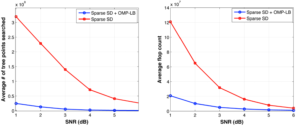
Figure 7: Computational complexity of sparsity-aware sphere decoder with (blue) and without (red) lower bounding technique, $m=n=40,l=5$, binary $\{0,1\}$ alphabet. The plot on the left compares average number of the tree points visited by the algorithm and the plot on the right compares average flop count.

VI An Application: Sparse Channel Estimation via Sparsity-Aware Sphere Decoding

In this section, we consider the application of the proposed sparsity-aware sphere decoding algorithm to the classical problem of sparse channel estimation (see, e.g., [30] and the references therein) and benchmark its performance against state-of-the-art alternative techniques. In estimation of sparse channel, impulse response of a channel having a given delay spread is described by only few non-zero taps and the estimation goal is to determine the values of those taps. This problem is often encountered in digital television and underwater acoustic communications [33] where the channel is naturally sparse, i.e., most of the channel energy is concentrated in few samples of the impulse response. Sparse estimation also comes up in ultra-wideband communications where only dominant multipath components are estimated, leading to a sparse characterization of the channel. In [30], the sparse channel estimation is formulated as an On-Off Keying (OOK) problem by decoupling the estimation into zero-tap detection followed by structured estimation of the values of the non-zero taps. Sphere decoding based zero-tap detection is among several methodologies considered in [30]. We show that our sparsity-aware sphere decoding algorithm enables performance matching that of the best previously developed schemes, and comes close to the fundamental performance limits.

VI-A System model

To learn the sparse channel impulse response, we transmit a known training sequence and observe the received signal. Let $\{u_{i}\}_{i=1}^{M}$ denote the finite-length training data sequence and let $u_{i}=0$ if $i>M$ or $i<0$. Assume that the channel has impulse response of length $L$ ( $>M$) and let ${\mathbf{h}}=[h_{1}~{}h_{2}~{}\ldots~{}h_{L}]^{T}$ denote the vector of the impulse response coefficients. The real-valued observations are collected into a vector ${\mathbf{x}}=[x_{1}~{}x_{2}~{}\ldots~{}x_{M+L-1}]$, and the relation between ${\mathbf{h}}$ and ${\mathbf{x}}$ is given by

$$x_{j}=\sum\limits_{i=1}^{L}~{}h_{i}u_{j-i+1}+\nu_{j},$$

for $j=1,\ldots,M+L-1$, with $\nu_{j}$ assumed to be independent, identically distributed zero-mean Gaussian noise of variance $\sigma^{2}$. Alternatively, (LABEL:appl1) can be written as the matrix-vector product

$${\mathbf{x}}={\mathbf{U}}{\mathbf{h}}+\boldsymbol{\nu},$$ (41)

where

$${\mathbf{U}}=\left[\begin{array}[]{ccc}u_{1}&&0\\ u_{2}&\ddots&\\ \vdots&\ddots&u_{1}\\ u_{M}&&u_{2}\\ &\ddots&\vdots\\ 0&&u_{M}\end{array}\right]\mbox{ and }\boldsymbol{\nu}=\left[\begin{array}[]{c}\nu_{1}\\ \nu_{2}\\ \vdots\\ \nu_{M+L-1}\end{array}\right].$$

Note that the channel vector can be represented as ${\mathbf{h}}=\mbox{diag}(h){\bf b}$, where ${\bf b}\in\{0,1\}^{L}$ has non-zero entries that indicate positions of the non-zero coefficients in ${\mathbf{h}}$, and diag($h$) is a diagonal matrix with entries from ${\mathbf{h}}$.

VI-B Sparsity-aware sphere decoder for channel estimation

Let $\hat{{\mathbf{h}}}$ denote the least-squares solution of (41). Then the zero-tap detection problem can be formulated as the following optimization [30]

$$\hat{{\bf b}}=\arg\underset{{\bf b}\in\{0,1\}^{L}}{\min}~{}\|{\mathbf{x}}-{\mathbf{U}}\mbox{diag}(\hat{h}){\bf b}\|^{2}.$$ (42)

In [30], the sphere decoding algorithm was used to solve (42) and find the point in the lattice ${\mathbf{U}}$diag($\hat{h}$) closest to ${\mathbf{x}}$. The solution $\hat{\bf b}$ is then used to refine the channel estimate $\hat{{\mathbf{h}}}$ and form a so-called structured estimate $\hat{{\mathbf{h}}}^{*}$ via the least-squares method. As an alternative, we employ the sparsity-aware sphere decoding from Section II-B to solve (42). The channel order, denoted by $m^{\#}$, is assumed known to the receiver. Then, (42) can be restated as

$$\hat{{\bf b}}=\arg\underset{{\bf b}\in\{0,1\}^{L}\atop\|{\bf b}\|_{0}~{}\leq~{}m^{\#}}{\min}~{}\|{\mathbf{x}}-{\mathbf{U}}\mbox{diag}(\hat{h}){\bf b}\|^{2}.$$ (43)

Remarks: Various methods for estimating the channel order at the receiver exist in literature. In [34], information theoretic criteria including Minimum Description Length (MDL) and Akaike Information Criterion (AIC) have been considered for determining the number of sources in sparse array processing [3]. In [35], a criterion for channel order estimation using least squares blind identification and equalization costs for SIMO channels was proposed. Often, information about the channel order is obtained from past history or data records.

VI-C Simulations

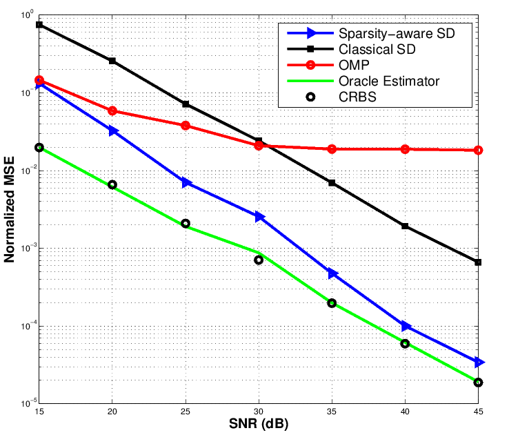
Figure 8: Comparison of normalized mean-squared error (MSE) for sparsity-aware SD, OMP and classical SD schemes for zero-tap detection, $L=20,M=6,m^{\#}=3$. The MSE of an oracle estimator and the CRLB for structured estimate are also plotted for comparison.

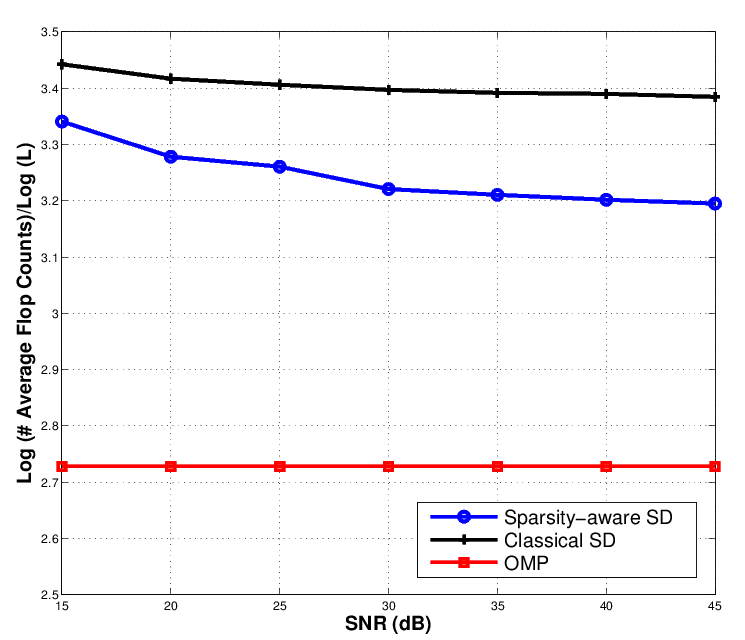
Figure 9: Comparison of complexity exponents for average flop counts of sparsity-aware SD, OMP and classical SD schemes for zero-tap detection, $L=20,M=6,m^{\#}=3$.

Performance of the sparsity-aware sphere decoding algorithm applied for sparse channel estimation is demonstrated in Fig. 8, where we plot the normalized mean-squared-error (MSE) of competing channel estimation schemes as a function of SNR. The normalized MSE is defined as MSE = $1/T\sum_{t=1}^{T}\|{\mathbf{h}}_{t}-\hat{{\mathbf{h}}}_{t}\|^{2}/\|{\mathbf{h}}_{t}\|^{2}$, where $T$ is the total number of Monte Carlo iterations and ${\mathbf{h}}_{t}$ and $\hat{{\mathbf{h}}}_{t}$ are the vectors of actual channel coefficients and their estimates in the $t^{th}$ iteration of the estimation procedure, respectively. The values of $L$, $M$ and the channel order $m^{\#}$ are $20$, $6$ and $3$, respectively. The training sequence is formed by taking $M$ samples of constant modulus. The non-zero coefficients of ${\mathbf{h}}_{t}$ are assumed to independent standard normal variables.

To solve the sparse channel estimation problem and obtain the MSE shown in Fig. 8, we employed the sparsity-aware sphere decoder from Section III with radius update for faster run times. The MSE performance of the classical sphere decoding algorithm and structured estimate obtained via orthogonal matching pursuit (OMP) [36] are among those shown in Fig 8. It is clear from this figure that sparsity-aware sphere decoder using knowledge of channel order performs significantly better than the classical sphere decoding adopted in [30]. The MSE of the oracle estimator and the theoretical performance limit in the form of Cramer Rao lower bound (CRLB) [30] are also plotted in the same figure. Oracle estimator is the structured least-square estimator with known locations of non-zero channel taps. In [37], it was shown that OMP matches the best performance among sparse channel estimation methods that use knowledge of true channel order. Clearly, over a wide range of signal-to-noise ratios (SNRs), the sparsity-aware sphere decoder significantly outperforms the OMP algorithm, with the performance gap increasing with SNR. In addition, we plot complexity exponents (evaluated using the average flop counts incurred by the algorithms applied to sparse channel estimation problem) in Fig. 9. It can be seen from this figure that sparsity-aware sphere decoding runs faster than the classical sphere decoder. The OMP algorithm is the fastest but its accuracy is inferior to sparsity-aware sphere decoding.

VII Conclusion

Sparsity-aware sphere decoder presented and analyzed in this paper has been motivated by the recent emergence of applications which require finding the solution to sparse integer least-squares problems. The sparsity-aware sphere decoding algorithm exploits sparsity information to prune nodes from the search tree that would have otherwise been visited by the classical sphere decoder. Imposing sparsity constraints requires minor additional computations, but due to more aggressive tree pruning, leads to significant improvements in complexity while improving accuracy. We analyzed computational complexity of the sparsity-aware sphere decoding algorithm and found its first and second-order moments (i.e., the mean and the variance of the random variable representing the complexity of the proposed algorithm). An application to sparse channel estimation demonstrated the efficacy of the algorithm.

To further reduce the computational complexity of the algorithm, we imposed a lower bound on a part of the objective function at each stage and used it to make the sphere constraint more restrictive. The lower bound was posed as an $\ell_{1}$-norm regularized relaxed version of the sparse integer least-squares problem, and efficiently computed using the orthogonal matching pursuit technique. As simulation results demonstrate, the proposed method may lead to significant computational savings over straightforward sparsity-aware sphere decoding.

As part of future work, in addition to first and second-order moments of the complexity of sparsity-aware sphere decoder analyzed in this manuscript, it would be beneficial to further characterize the complexity by, for example, exploring higher-order moments and its tail distribution. Moreover, for the lower-bound based speed-up of the algorithm, it is of interest to explore alternative relaxations of integer least-squares problems as well as investigate fast methods for solving such relaxations. Finally, applying the proposed techniques to solve various practical problems and exploiting structural properties of those problems to further improve the complexity and performance are of potential interest.

References

- [1] E. Agrell, T. Eriksson, A. Vardy and K. Zeger, “Closest lattice point search in lattices,” IEEE Trans. Info. Theory, vol. 48, no. 8, pp.2201-2214, Aug. 2002.
- [2] H. Zhu and G. B. Giannakis, “Exploiting sparse user activity in multiuser detection,” IEEE Trans. on Signal Processing, vol. 59, no. 2, pp: 454-465, February 2011.
- [3] T. Yardbidi, J. Li, P. Stoica, and L. N. Cattafesta III, “Sparse representation and sphere decoding for array signal processing,” Digital Signal Processing, doi:10.1016/j.dsp.2011.10.006 (in press), 2011.
- [4] Z. Li and W. Trappe, “Collusion-resistant fingerprints from WBE sequence sets,” IEEE International Conference on Communications, vol.2, pp. 1336-1340, 16-20 May 2005.
- [5] R. Pique-Regi, J. Monso-Varona, A. Ortega, R. C. Seeger, T. J. Triche, and S. Asgharzadeh, “Sparse representation and Bayesian detection of genome copy number alterations from microarray data,” Bioinformatics, vol. 24, no. 8, pp: 309-318, 2008.
- [6] M. Grotschel, L. Lovasz, and A. Schriver, “Geometric Algorithms and Combinatorial Optimization,” Springer Verlag, 2nd edition, 1993.
- [7] U. Fincke and M. Pohst, “Improved methods for calculating vectors of short length in a lattice, including a complexity analysis,” Math. Comput., vol. 44, pp. 463-471, Apr. 1985.
- [8] H. Vikalo, Sphere decoding algorithms for digital communications, PhD Thesis, Stanford University, 2003.
- [9] B. Hassibi and H. Vikalo, “On the sphere-decoding algorithm I. Expected complexity,” IEEE Trans. on Signal Processing, vol. 53, no. 8, pp. 2806-2818, Aug. 2005.
- [10] H. Vikalo and B. Hassibi, ”On the sphere-decoding algorithm II. Generalizations, second-order statistics, and applications to communications,” IEEE Trans. Signal Processing, vol. 53, no. 8, pp. 2819-2834, Aug. 2005.
- [11] Z. Tian, G. Leus, and V. Lottici, “Detection of sparse signals under finite-alphabet constraints,” Proc. of ICASSP, pp: 2349-2352, 2009.
- [12] H. Vikalo and B. Hassibi, “On joint detection and decoding of linear block codes on Gaussian vector channels,” IEEE Trans. on Signal Processing, vol. 54, no. 9, pp. 3330-3342, September 2006.
- [13] A. Younis, R. Mesleh, H. Haas, and P. Grant, “Reduced Complexity Sphere Decoder for Spatial Modulation Detection Receivers,” in Proc. of IEEE Globecom, 2010, Miami, USA, 2010, pp. 1-5.
- [14] J. Jalden and B. Ottersten, “On the complexity of sphere decoding in digital communications,” IEEE Transactions on Signal Processing, vol. 53, no. 4, pp. 1474- 1484, April 2005.
- [15] D. Seethaler, J. Jalden, C. Studer, and H. Bolcskei, “On the Complexity Distribution of Sphere Decoding,” IEEE Transactions on Information Theory, vol. 57, no. 9, pp. 5754-5768, Sept. 2011.
- [16] D. Seethaler and H. Bolcskei, “Performance and complexity analysis of infinity-norm sphere-decoding,” IEEE Trans. Inf. Theory, vol. 56, no. 3, pp. 1085–1105, Mar. 2010.
- [17] A. Younis, M. Di Renzo, R. Mesleh, H. Haas, “Sphere Decoding for Spatial Modulation,” in Proc. of IEEE ICC, 2011, Kyoto, Japan, 2011.
- [18] S. S. Chen, Basis Pursuit, PhD Thesis, Stanford University, 1995.
- [19] S. S. Chen, D. L. Donoho, and M. A. Saunders, ”Atomic decomposition by basis pursuit,” SIAM Journal on Scientific Computing, vol. 20, no. 1, 1999, pp. 33-61.
- [20] E. Candes, J. Romberg, and T. Tao, ”Robust uncertainty principles: Exact signal reconstruction from highly incomplete frequency information,” IEEE Trans. on Info. Theory, 52(2), Feb. 2006, pp. 489-509.
- [21] E. Candes and T. Tao, ”Near optimal signal recovery from random projections: Universal encoding strategies,” IEEE Transactions on Information Theory, 52(12), December 2006, pp. 5406-5425.
- [22] D. Donoho, ”Compressed sensing,” IEEE Trans. on Info. Theory, 52(4), April 2006, pp. 1289-1306.
- [23] D. Donoho and Y. Tsaig, ”Extensions of compressed sensing,” Sig. Proc., 86(3), 2006, pp. 533-548.
- [24] E. J. Candes, ”Compressive sampling,” Proc. of the Intern. Congress of Mathem., Madrid, Spain, 2006.
- [25] A. D. Murugan, H. E. Gamal, M. O. Damen, and G. Caire, “A unified framework for tree search decoding: Rediscovering the sequential decoder,” IEEE Trans. Inf. Theory, vol. 52, no. 3, pp. 933–953, Mar 2006.
- [26] B. Steingrimsson, L. Zhi-Quan, and K. Wong, “Soft quasi-maximum-likelihood detection for multiple- antenna wireless channels,” IEEE Transactions on Signal Processing, vol.51, no.11, pp. 2710- 2719, Nov 2003.
- [27] G. Zhan and P. Nilsson, “Reduced complexity Schnorr-Euchner decoding algorithms for MIMO systems,” IEEE Communications Letters, vol.8, no.5, pp. 286- 288, May 2004.
- [28] L. G. Barbero and J. S. Thompson, “Fixing the Complexity of the Sphere Decoder for MIMO Detection,” IEEE Transactions on Wireless Communications, vol.7, no.6, pp.2131-2142, June 2008.
- [29] Z. Li and W. Trappe, “WBE-based anti-colusion fingerprints: Design and detection,” Studies in Computational intelligence, Springer-Verlag, Berlin Heidelberg 2010, pp: 305-335 (editors : H. T. Sencar, S. Velastin, N. Nikolaidis, and S. Lian).
- [30] C. Carbonelli, S. Vedantam, and U. Mitra, “Sparse channel estimation with zero-tap estimation,” IEEE Trans. on Wireless Communications, vol. 6, no. 5, pp. 1743-1763, May 2007.
- [31] T. Worsch, “Lower and upper bounds for (sums of) binomial coefficients,” Technical Report 31/94, Universitaat Karlsruhe, Fakultat fuer Informatik, 1994. URL: http://digbib.ubka.unikarlsruhe.de/volltexte/181894.
- [32] M. Stojnic, H. Vikalo, and B. Hassibi, “Speeding up the sphere decoder with and SDP inspired lower bounds,” IEEE Trans. on Sig. Proc., vol. 56, no. 2, pp. 712-726, Feb. 2008.
- [33] C. R. Berger, S. Zhou, J. C. Preisig, and P. Willett, “Sparse channel estimation for multicarrier underwater acoustic communication: From subspace methods to compressed sensing,” in Proc. of MTS/IEEE OCEANS conference, Bremen, Germany, May 11-14, 2009.
- [34] E. Fishler and H. V. Poor, “Estimation of the number of sources in unbalanced arrays via information theoretic criteria,” IEEE Trans. Signal Processing, vol. 53, no. 9, pp. 3543-3553, Sep. 2005.
- [35] J. Vía, I. Santamaría, and J. Pérez, “Effective channel order estimation based on combined identification/ equalization,”IEEE Trans. Signal Process., vol. 54, no. 9, pp. 3518–3526, Sep. 2006.
- [36] J. A Tropp and A. C. Gilbert, “Signal recovery from random measurements via orthogonal matching pursuit,” IEEE Transactions on Information Theory, vol. 53, no. 12, pp: 4655 - 4666, December 2007.
- [37] F. Wan, U. Mitra, and A. Molisch, “The modified iterative detector/estimator algorithm for sparse channel estimation,” in Proc. IEEE OCEANS Conf. , Seattle, WA, Sep. 2010, DOI: 10.1109/OCEANS.2010.5664395.
- [38] S. Barik and H. Vikalo, “Expected complexity of sphere decoding for sparse integer least-square problems,” Proc. IEEE International Conference on Acoustic, Speech, and Signal Processing, Vancouver, May 2013.