Large deviations in the alternating mass harmonic chain

Abstract

We extend the work of Kannan et al. and derive the cumulant generating function for the alternating mass harmonic chain consisting of $N$ particles and driven by heat reservoirs. The main result is a closed expression for the cumulant generating function in the thermodynamic large $N$ limit. This expression is independent of $N$ but depends on whether the chain consists of an even or an odd number of particles, in accordance with the results obtained by Kannan el al. for the heat current. This result is in accordance with the absence of local thermodynamic equilibrium in a linear system.

.

I Introduction

There is a current interest in fluctuating small systems in contact with heat reservoirs and driven by external forces. This focus is driven by the recent possibilities of direct manipulation of nano systems and bio molecules. These techniques also permit direct experimental access to the probability distributions for the work or heat exchanged with the environment Trepagnier et al. (2004); Collin et al. (2005); Tietz et al. (2006); Blickle et al. (2006); Wang et al. (2002); Imparato et al. (2007); Douarche et al. (2006); Garnier and Ciliberto (2007); Imparato et al. (2008). Moreover, these single molecule techniques have also yielded access to the so called fluctuation theorems, which relate the probability of observing entropy-generated trajectories, with that of observing entropy-consuming trajectories Jarzynski (1997); Kurchan (1998); Gallavotti (1996); Crooks (1999, 2000); Seifert (2005a, b); Evans et al. (1993); Evans and Searles (1994); Gallavotti and Cohen (1995); Lebowitz and Spohn (1999); Gaspard (2004); Imparato and Peliti (2006); van Zon and Cohen (2003a); van Zon et al. (2004); van Zon and Cohen (2003b, 2004); Speck and Seifert (2005). As a result there is a general renewed theoretical interest in small non equilibrium systems.

In the context of non equilibrium systems the well-known fluctuation-dissipation theorem, relating response to fluctuations close to equilibrium has been generalized to the so-called asymptotic fluctuation theorem (AFT) valid also far from equilibrium Evans et al. (1993); Evans and Searles (1994); Gallavotti and Cohen (1995); Lebowitz and Spohn (1999); Kurchan (1998); Crooks (1999); Seifert (2005a). The AFT, which has been demonstrated under quite general conditions, implies for the cumulant generating function (CGF) the fundamental symmetry

$$\mu(\lambda)=\mu(\beta_{1}-\beta_{2}-\lambda).$$ (1)

The CGF, $\mu(\lambda)$, is defined at long times $t$ according to

$$\langle\exp(\lambda Q(t)\rangle\sim\exp(t\mu(\lambda)),$$ (2)

where $Q(t)$ is the accumulated heat transferred to the system from a reservoir in the time span $t$. Here $\beta_{1}=1/T_{1}$ and $\beta_{2}=1/T_{2}$ are the inverse temperatures of the heat reservoirs driving the non equilibrium process and $\langle\cdots\rangle$ denotes a non equilibrium ensemble average. Normalization implies $\mu(0)=0$ and the AFT in (1) in particular yields $\mu(\beta_{1}-\beta_{2})=0$. In general $\mu(\lambda)$ is a downward convex function passing through $\lambda=0$ and $\lambda=\beta_{1}-\beta_{2}$. $\mu(\lambda)$ is, moreover, bounded by branch points at $\lambda_{+}$ and $\lambda_{-}$.

Recently, there has been focus on the explicit evaluation of $\mu(\lambda)$ for deterministic systems driven by Langevin type heat bath in order to verify the AFT and at the same time determine how system dependent properties enter in the form of $\mu(\lambda)$. Little is known about $\mu(\lambda)$ in the case of interacting or random systems and the focus has therefore been on tractable linear systems. In a series of papers Saito and Dhar and Kundu et al. Saito and Dhar (2007); Kundu et al. (2011), see also Sabhapandit (2011, 2012); Fogedby and Imparato (2012), have discussed the driven harmonic chain. Here one finds that $\mu(\lambda)$ is a functional of

$$f(\lambda)=T_{1}T_{2}\lambda(\beta_{1}-\beta_{2}-\lambda),$$ (3)

where inspection reveals that $f(\lambda)$ is invariant under the AFT symmetry in (1). The functional in the case of the deterministic harmonic linear chain has the generic form

$$\mu(\lambda)=-\frac{1}{2}\int\frac{d\omega}{2\pi}\ln\bigg{[}1+T(\omega)f(\lambda)\bigg{]},$$ (4)

where $T(\omega)$ is a model dependent transmission matrix. In linear systems the heat is transported ballistically. Local equilibrium cannot be established and Fourier’s law does not hold Bonetto et al. (2000). This is reflected in the form of $\mu(\lambda)$ which is independent of the system size.

In the case of a simple $N$ particle unit mass harmonic chain with inter particle coupling $\kappa$, attached to walls at the ends, and driven by two heat reservoirs with common damping $\Gamma$, one obtains the transmission matrix Saito and Dhar (2007); Kundu et al. (2011); Fogedby and Imparato (2012)

$$T(\omega)=(2\Gamma\omega)^{2}|G_{1N}(\omega)|^{2},$$ (5)

$$G_{1N}(\omega)=\frac{\kappa\sin p}{\Omega^{2}\sin(N-1)p-2\kappa\Omega\sin(N-2)p+\kappa^{2}\sin(N-3)p},$$ (6)

$$\Omega=-\omega^{2}+2\kappa-i\Gamma\omega,$$ (7)

$$\omega^{2}=4\kappa\sin^{2}p/2.$$ (8)

Here (5) defines $T$ in terms of the the transmission end-to-end Green’s function $G_{1N}$ given in (6). The above results have been analyzed in detail in Saito and Dhar (2007); Kundu et al. (2011); Fogedby and Imparato (2012). Here we just remark that the ballistic lattice waves transporting the heat give rise to the resonance structure in the denominator in (6). The coupling to the heat reservoirs only enters in $\Omega$ in (7). Finally, the wave number $p$ is confined to the first Brillouin zone $|p|\leq\pi$, yielding the frequency band $|\omega|\leq 2\sqrt{\kappa}$.

A natural and simple extension of the equal mass harmonic chain is the harmonic chain with alternating masses. In condensed matter this is the well-known case of a phonon system with a basis. In this case the dispersion law (8) breaks up into an acoustic branch and an optical branch, see e.g. Ashcroft and Mermin (1976). In both case the heat is transmitted ballistically but shared between the acoustic and optical phonons.

In recent work Kannan et al. Kannan et al. (2012) have considered this case and have in detail analysed the non equilibrium steady state of an alternating mass harmonic chain Casher and Lebowitz (1971); O’Connor and Lebowitz (1974); further references to work on the alternating mass chain can be found in Kannan et al. (2012). Like in the equal mass case Rieder et al. (1967); Nakazawa (1970), the position and momentum steady state distribution exhibits a Gaussian form with correlation matrix given by the static position-position, position-momentum, and momentum-momentum correlations. Defining the local kinetic temperature $T_{n}$ according to (note that $k_{\text{B}}=1$) $T_{n}=\langle p_{n}^{2}\rangle/m_{n}$, where $p_{n}$ is the momentum and $m_{n}$ the mass associated with the n-th site, Kannan et al. find, surprisingly, that the local temperature $T_{n}$ oscillates with period 2; these oscillations even persist in the thermodynamic limit; in the equilibrium case for $T_{1}=T_{2}=T$ the local temperature $T_{n}$ locks onto $T$ in accordance with the equipartion theorem. Kannan et al. Kannan et al. (2012) also discuss the thermodynamic limit $N\rightarrow\infty$ and find exact expressions for the local temperature profile $T_{n}$ and the heat current $\langle Q\rangle/t$. They also find that these expressions depend on whether the chain is composed of an even or odd number of particles.

In the present paper we extend the work of Kannan et al. regarding the large $N$ limit of the heat current and discuss the cumulant generating function $\mu(\lambda)$ (CGF). The CGF yields the full heat distribution in the long time limit; note that the heat current is given by the first term in a cumulant expansion of (2), i.e., $\langle Q\rangle/t=(d\mu(\lambda)/d\lambda)_{\lambda=0}$. Referring to the results in Fogedby and Imparato (2012); Saito and Dhar (2007); Kundu et al. (2011), the central quantity in the evaluation of the CGF is the transmission Green’s function $G_{1N}(\omega)$ describing the propagation of ballistic modes across a chain of size $N$. We consider the CGF and determine the transmission matrix $T(\omega)$ entering in the expression (4). As anticipated the structure of $T(\omega)$ exhibits the two branch structure of the phonon spectrum, both the acoustic and optical branches contributing to $T(\omega)$. Finally, we derive a close expression for the CGF in the large $N$ limit. This constitutes the main and new result in the present paper. In accordance with the absence of local thermodynamic equilibrium the large $N$ expression for the CGF is manifestly independent of $N$.

The paper is organised in the following manner. In Sec. II we present the model under scrutiny, i.e., the alternating mass chain. In Sec. III we set up the necessary analytical apparatus. In Sec. IV we introduce the transmission end-to-end Greens function which incorporates the model dependent component of the CGF. Section  V contains the main result in the present paper, namely a derivation of the CGF in the large $N$ limit. Section  VI is devoted to a discussion of the CGF in the large $N$ limit. For completion this section also includes a discussion of the transmission matrix and the large deviation function. Section  VII is devoted to a conclusion. The issue of deriving an expression for the end-to-end Green’s function suitable for our needs is deferred to an Appendix.

II Model

We consider an alternating mass harmonic chain attached to a wall at the end points. The spring constant is denoted by $\kappa$ and the two masses in the unit cell are $m$, the smaller mass, and $M$, the larger mass. The end particles are driven by heat reservoirs at temperatures $T_{1}$ and $T_{2}$, characterised by the damping constant $\Gamma$. Kannan et al. Kannan et al. (2012) use a determinantal approach in analysing the stochastic dynamics. We have found it convenient for our purposes to use an equation of motion approach.We readily distinguish two cases depending on the boundary conditions. In case A an integer number of unit cells fits in between the walls, corresponding to an even number of particles; in case B a half unit cell is in contact with the right wall, corresponding to an odd number of particles. In Fig. 1 we have depicted the two cases and the appropriate unit cell.

Denoting the displacement of the particle with mass $m$ in the n-th unit cell by $u_{n}$ and the displacement of the particle with mass $M$ by $w_{n}$, we obtain in bulk the coupled equations of motion

$$m\ddot{u}_{n}=\kappa(w_{n}+w_{n-1}-2u_{n}),$$ (9)

$$M\ddot{w}_{n}=\kappa(u_{n}+u_{n+1}-2w_{n});$$ (10)

here a dot denotes a time derivative.

Case A (even): From Fig. 1 it follows that the coupling to the heat reservoirs is described by the Langevin equations

$$m\ddot{u}_{1}=-\Gamma\dot{u}_{1}+\kappa(w_{1}-2u_{1})+\xi_{1},$$ (11)

$$M\ddot{w}_{N}=-\Gamma\dot{w}_{N}+\kappa(u_{N}-2w_{N})+\xi_{N},$$ (12)

where $N$ is the number of unit cells, corresponding to $2N$ particles of either mass, i.e., an even number of particles.

Case B (odd): According to Fig. 1, (12) is replaced by

$$M\ddot{u}_{N+1}=-\Gamma\dot{u}_{N+1}+\kappa(w_{N}-2u_{N+1})+\xi_{N},$$ (13)

for $N$ unit cells with only one particle of mass $m$ in the $(N+1)$-th unit cell, corresponding to an odd number of particles. Finally, the noises $\xi_{1}$ and $\xi_{N}$, characterising the heat reservoirs, are correlated according to

$$\langle\xi_{1}(t)\xi_{1}(t^{\prime})\rangle=2\Gamma T_{1}\delta(t-t^{\prime}),$$ (14)

$$\langle\xi_{N}(t)\xi_{N}(t^{\prime})\rangle=2\Gamma T_{2}\delta(t-t^{\prime}).$$ (15)

The above equations of motion define the dynamics of the chain and the stochastic coupling to the heat reservoirs at temperatures $T_{1}$ and $T_{2}$.

Focussing on the reservoir at temperature $T_{1}$ the fluctuating force is given by $-\Gamma\dot{u}_{1}+\xi_{1}$. Consequently, the rate of work or heat flux has the form, denoting $Q\equiv Q_{1}$,

$$\dot{Q}=\dot{u}_{1}(-\Gamma\dot{u}_{1}+\xi_{1}).$$ (16)

With respect to the CGF the central quantity in the analysis is, however, the total heat transmitted to the system during a finite time interval $t$, i.e.,

$$Q(t)=\int_{0}^{t}d\tau\dot{u}_{1}(-\Gamma\dot{u}_{1}+\xi_{1}).$$ (17)

The heat $Q(t)$ is fluctuating and the issue is to determine its probability distribution $P(Q,t)=\langle\delta(Q-Q(t))\rangle$, where $\langle\cdots\rangle$ denotes an ensemble average with respect to $\xi_{1}$ and $\xi_{N}$. In terms of the characteristic function $\langle\exp(\lambda Q(t)\rangle$ we have by a Laplace transform Gradshteyn and Ryzhik (1965)

$$P(Q,t)=\int_{-i\infty}^{i\infty}\frac{d\lambda}{2\pi i}e^{-\lambda Q}\langle e^{\lambda Q(t)}\rangle,$$ (18)

where at long times $\langle\exp(\lambda Q(t)\rangle\sim\exp(t\mu(\lambda))$. Note that $Q(t)$ is unbounded and only the time scaled heat $Q(t)/t$ is endowed with large deviation properties Touchette (2009); den Hollander (2000).

III Analysis

The heat reservoirs drive the chain into a stationary non equilibrium state. The heat is transported ballistically by the acoustic and optical phonons. The only damping mechanism is associated with the heat reservoirs and sets a time scale given by $1/\Gamma$. Consequently, at long times compared to $1/\Gamma$ we can ignore the initial preparation and employ the Fourier transform,

$$u_{n}(t)=\int\frac{d\omega}{2\pi}\exp(-i\omega t)u_{n}(\omega),$$ (19)

$$w_{n}(t)=\int\frac{d\omega}{2\pi}\exp(-i\omega t)w_{n}(\omega).$$ (20)

Proceeding with an equation of motion approach, introducing

$$\tilde{\Omega}_{1}=-m\omega^{2}+2\kappa,$$ (21)

$$\tilde{\Omega}_{2}=-M\omega^{2}+2\kappa,$$ (22)

the bulk equation of motion (9) and (10) take the form

$$\tilde{\Omega}_{1}u_{n}=\kappa(w_{n}+w_{n-1}),$$ (23)

$$\tilde{\Omega}_{2}w_{n}=\kappa(u_{n}+u_{n+1}).$$ (24)

Commonly, for systems with periodic boundary conditions one searches for plane wave solutions of the form $u_{n},w_{n}\sim\exp(ipn)$ and readily finds the dispersion laws for acoustic and optical phonons Ashcroft and Mermin (1976). In the present context for a finite chain coupled to heat baths, it is more convenient to proceed in a renormalisation group fashion by diluting the degrees of freedom. Thus eliminating every second site we obtain from (23) and (24) bulk equations referring to each separate sublattice,

$$\tilde{\Omega}_{1}\tilde{\Omega}_{2}u_{n}=\kappa^{2}(u_{n+1}+u_{n-1}+2u_{n}),$$ (25)

$$\tilde{\Omega}_{1}\tilde{\Omega}_{2}w_{n}=\kappa^{2}(w_{n+1}+w_{n-1}+2w_{n}).$$ (26)

Searching for plane wave solutions, $u_{n},w_{n}\sim\exp(ipn)$, we find the common dispersion law for the two sublattices,

$$\tilde{\Omega}_{1}\tilde{\Omega}_{2}=2\kappa^{2}(1+\cos p),$$ (27)

or inserting $\tilde{\Omega}_{1}$ and $\tilde{\Omega}_{2}$ from (21) and (22) the two branches

$$\omega_{1}^{2}=\kappa\frac{m+M-s}{mM},$$ (28)

$$\omega_{2}^{2}=\kappa\frac{m+M+s}{mM},$$ (29)

$$s=\sqrt{m^{2}+M^{2}+2mM\cos p}.$$ (30)

For the acoustic branch the $\omega$ range is $0<|\omega|<\sqrt{2\kappa/M}$; for the optical branch $\sqrt{2\kappa/m}<|\omega|<\sqrt{2\kappa(m+M)/mM}$. The wave number range is $|p|\leq\pi$. The dispersion laws, moreover, locks $\omega$ onto $p$ in the Fourier integrals over $\omega$ in for example (19) and (20).

For later purposes we also need the inverse density of phonon states

$$\rho_{1}(p)=\frac{d\omega_{1}}{dp}=\frac{\kappa\sin p}{2\omega_{1}s},$$ (31)

$$\rho_{2}(p)=\frac{d\omega_{2}}{dp}=\frac{\kappa\sin p}{2\omega_{2}s},$$ (32)

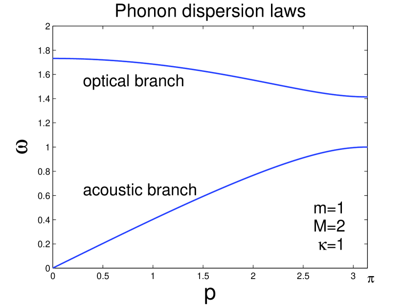
Figure 2: We depict the acoustic and optical phonon branches in a plot of $\omega$ versus $p$ given in (28), (29), and (30). The wavenumber range is $0<p<\pi$. We have set $m=1$, $M=2$, and $\kappa=1$.

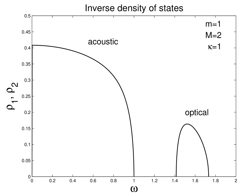
Figure 3: We depict the inverse density of states, $\rho_{n}=d\omega_{n}/dp$, for the acoustic and optical branches, respectively, given by (31) and (32). We plot $\rho_{n}$ as function of $\omega$ in order to exhibit the band gap. We have set $m=1$, $M=2$, and $\kappa=1$.

referring to the acoustic and optical branches, respectively. In Figs. 2 and 3 we have depicted the phonon dispersion laws and the inverse density of states as function of $\omega$, showing the gap between the acoustic and optical branches. We have chosen the parameter values $m=1$, $M=2$, and $\kappa=1$.

Introducing

$$\Omega_{1}=-m\omega^{2}+2\kappa-i\omega\Gamma,$$ (33)

$$\Omega_{2}=-M\omega^{2}+2\kappa-i\omega\Gamma.$$ (34)

the coupling to the reservoirs in case A (even) and B (odd) is described by

$$\Omega_{1}u_{1}=\kappa w_{1}+\xi_{1},$$ (35)

$$\Omega_{2}w_{N}=\kappa u_{N}+\xi_{N},$$ (36)

and

$$\Omega_{1}u_{1}=\kappa w_{1}+\xi_{1},$$ (37)

$$\Omega_{1}u_{N+1}=\kappa w_{N}+\xi_{N},$$ (38)

respectively.

The clamping of the chain to the walls gives rise to a dynamical coupling of the $u$ and $w$ sublattices. The $u$ and $w$ displacements driven by the noise inputs at the ends can be expressed in the form

$$u_{n}^{\text{A},\text{B}}=G_{n1}^{\text{A},\text{B}}\xi_{1}+G_{nN}^{\text{A},\text{B}}\xi_{N},$$ (39)

$$w_{n}^{\text{A},\text{B}}=F_{n1}^{\text{A},\text{B}}\xi_{1}+F_{nN}^{\text{A},\text{B}}\xi_{N},$$ (40)

where $G^{\text{A},\text{B}}$ and $F^{\text{A},\text{B}}$ are Green’s functions describing the propagation of ballistic modes from the end points to the n-th unit cell in the two cases.

IV Transmission Green’s function

Since according to (16) we inject heat at the site $u_{1}$ the relevant transmission end-to-end Green’s function is $G_{1N}^{\text{A},\text{B}}$. In the appendix we have, using an equation of motion approach, evaluated the Green’s functions entering in (39) and (40). We stress that our derivation is in complete agreement with Kannan et al. Kannan et al. (2012), who use an equivalent determintal approach. Extracting the expressions from the appendix with a slight change in notation ($D^{\text{A}}=D_{1}^{\text{A}}$) we have

$$G_{1N}^{\text{A}}(\omega)=\frac{\kappa_{\text{A}}(\omega)\sin p}{D^{\text{A}}(\omega)},$$ (41)

$$G_{1N}^{\text{B}}(\omega)=\frac{\kappa_{\text{A}}(\omega)\sin p}{D^{\text{B}}(\omega)}.$$ (42)

We note that the end-to-end Green’s functions have the same structure as (6) in the case of a simple chain. From the appendix we also have

$$D^{\text{A}}(\omega)=\Omega_{\text{A}}\Omega_{\text{C}}\sin(N-1)p-(\Omega_{\text{A}}\kappa_{\text{D}}+\Omega_{\text{C}}\kappa_{\text{A}})\sin(N-2)p+\kappa_{\text{A}}\kappa_{\text{D}}\sin(N-3)p,$$ (43)

$$D^{\text{B}}(\omega)=\Omega_{\text{A}}^{2}\sin(N-1)p-2\Omega_{\text{A}}\kappa_{\text{A}}\sin(N-2)p+\kappa_{\text{A}}^{2}\sin(N-3)p,$$ (44)

where

$$\Omega_{\text{A}}=\Omega_{1}-\kappa^{2}/\tilde{\Omega}_{2},$$ (45)

$$\Omega_{\text{C}}=(\Omega_{2}/\kappa)(\tilde{\Omega}_{1}-\kappa^{2}/\tilde{\Omega}_{2})-\kappa,$$ (46)

$$\kappa_{\text{A}}(\omega)=\kappa^{2}/\tilde{\Omega}_{2},$$ (47)

$$\kappa_{\text{D}}(\omega)=\kappa\Omega_{2}/\tilde{\Omega}_{2},$$ (48)

Here the frequency dependent parameters $\tilde{\Omega}_{1}$, $\tilde{\Omega}_{2}$, $\Omega_{1}$, and $\Omega_{2}$ are given by (21), (22), (33), and (34).

We note that the end-to-end Green’s functions have a complex $\omega$ dependence owing to the coupling of the two sublattices, yielding a frequency dependent coupling strength $\kappa_{\text{A}}(\omega)$ as well as denominators $D^{\text{A}}(\omega)$ and $D^{\text{B}}(\omega)$ depending on whether we are in case A (even) or case B (odd). Detailed inspection reveals that these expressions are identical to corresponding expressions in Kannan et al. Kannan et al. (2012). A tedious analysis, setting $m=M$ and noting that the number of particles is twice the number of unit cells, also leads to the expression (6) to (8) for the simple chain.

V Cumulant generating function in the large $N$ limit

The derivation of the cumulant generating function (CGF) proceeds like in Fogedby and Imparato (2012), see also Saito and Dhar (2007); Kundu et al. (2011), with some added technicalities due to the two band structure. The central model-dependent quantity is the end-to-end Green’s functions given in (41) and (42). Here $\kappa_{\text{A}}(\omega)$ in (47) is an effective frequency dependent coupling strength; the denominators $D^{\text{A}}(\omega)$ and $D^{\text{B}}(\omega)$ in (43) and (44) describe the resonance structure of the chain.

The cumulant generating function CGF is given by the generic expression (4). In the present case, referring to case A (even) and case B (odd), we have

$$\mu^{\text{A},\text{B}}(\lambda)=-\frac{1}{2}\int\frac{d\omega}{2\pi}\ln\bigg{[}1+T^{\text{A},\text{B}}(\omega)f(\lambda)\bigg{]},$$ (49)

$$f(\lambda)=T_{1}T_{2}\lambda(\beta_{1}-\beta_{2}-\lambda),$$ (50)

where the transmission matrix has the form

$$T^{\text{A},\text{B}}(\omega)=(2\Gamma\omega)^{2}|G^{\text{A},\text{B}}_{1N}(\omega)|^{2};$$ (51)

note that in (49) the $\omega$ integration is over both acoustic and optical bands. Inserting the density of states (31) and (32) we obtain in particular

$$\mu^{\text{A},\text{B}}(\lambda)=-\int_{0}^{\pi}\frac{dp}{2\pi}\sum_{n=1,2}\rho_{n}\ln\bigg{[}1+(2\Gamma\omega_{n})^{2}|G^{\text{A},\text{B}}_{1N}(\omega_{n})|^{2}\bigg{]},$$ (52)

where $n=1,2$ refers to the acoustic and optical bands, respectively.

In order to extract the $N$ dependence of the CGF we note that $N$ only enters in the denominators $D^{\text{A},\text{B}}$ in (43) and (44). We proceed using the method in Fogedby and Imparato (2012); Kannan et al. (2012); Roy and Dhar (2008) by expressing $D^{\text{A},\text{B}}$ in the compact form

$$D^{\text{A},\text{B}}=\tilde{A}^{\text{A},\text{B}}\sin(N-1)p+\tilde{B}^{\text{A},\text{B}}\sin(N-2)p+\tilde{C}^{\text{A},\text{B}}\sin(N-3)p,$$ (53)

where from (43) and (44)

$$\tilde{A}^{\text{A}}=\Omega_{\text{A}}\Omega_{\text{C}},~{}~{}\tilde{B}^{\text{A}}=-\Omega_{\text{A}}\kappa_{\text{D}}-\Omega_{\text{C}}\kappa_{\text{A}},~{}~{}\tilde{C}^{\text{A}}=\kappa_{\text{A}}\kappa_{\text{D}},$$ (54)

$$\tilde{A}^{\text{B}}=\Omega_{\text{A}}^{2},~{}~{}\tilde{B}^{\text{B}}=-2\Omega_{\text{A}}\kappa_{\text{A}},~{}~{}\tilde{C}^{\text{B}}=\kappa_{\text{A}}^{2}.$$ (55)

Next expanding the sines in (53) we have

$$D^{\text{A},\text{B}}=a^{\text{A},\text{B}}\sin Np-b^{\text{A},\text{B}}\cos Np,$$ (56)

$$a^{\text{A},\text{B}}=\tilde{A}^{\text{A},\text{B}}\cos p+\tilde{B}^{\text{A},\text{B}}\cos 2p+\tilde{C}^{\text{A},\text{B}}\cos 3p,$$ (57)

$$b^{\text{A},\text{B}}=\tilde{A}^{\text{A},\text{B}}\sin p+\tilde{B}^{\text{A},\text{B}}\sin 2p+\tilde{C}^{\text{A},\text{B}}\sin 3p.$$ (58)

Further, expanding the norm squared, we finally obtain

$$|D^{\text{A},\text{B}}|^{2}=\frac{1}{2}\bigg{[}L^{\text{A},\text{B}}-M^{\text{A},\text{B}}\cos 2Np-C^{\text{A},\text{B}}\sin 2Np\bigg{]},$$ (59)

or

$$|D^{\text{A},\text{B}}|^{2}=\frac{1}{2}\bigg{[}L^{\text{A},\text{B}}-K^{\text{A},\text{B}}\cos(2Np-\phi^{\text{A},\text{B}})\bigg{]},$$ (60)

where we have introduced the parameters

$$L^{\text{A},\text{B}}=|a^{\text{A},\text{B}}|^{2}+|b^{\text{A},\text{B}}|^{2},$$ (61)

$$M^{\text{A},\text{B}}=|a^{\text{A},\text{B}}|^{2}-|b^{\text{A},\text{B}}|^{2},$$ (62)

$$C^{\text{A},\text{B}}=a^{\text{A},\text{B}}(b^{\text{A},\text{B}})^{\ast}+(a^{\text{A},\text{B}})^{\ast}b^{\text{A},\text{B}},$$ (63)

$$K^{\text{A},\text{B}}=\sqrt{(M^{\text{A},\text{B}})^{2}+(C^{\text{A},\text{B}})^{2}},$$ (64)

$$\tan\phi^{\text{A},\text{B}}=\frac{C^{\text{A},\text{B}}}{M^{\text{A},\text{B}}}.$$ (65)

Since the norm of the cosine is less than one, it follows from (60) that the upper and lower bounds of $|D^{\text{A},\text{B}}|^{2}$ are given by $(L^{\text{A},\text{B}}+K^{\text{A},\text{B}})/2$ and $(L^{\text{A},\text{B}}-K^{\text{A},\text{B}})/2$, respectively. Hence, from (51) it follows that the upper and lower bounds of $T^{\text{A},\text{B}}(\omega)$ are given by

$$T^{\text{A},\text{B}}_{\text{max}}(\omega)=2\frac{(2\Gamma\omega\kappa_{\text{A}}\sin p)^{2}}{L^{\text{A},\text{B}}-K^{\text{A},\text{B}}},$$ (66)

$$T^{\text{A},\text{B}}_{\text{envelope}}(\omega)=2\frac{(2\Gamma\omega\kappa_{\text{A}}\sin p)^{2}}{L^{\text{A},\text{B}}+K^{\text{A},\text{B}}},$$ (67)

respectively. The final step in obtaining a large $N$ expression for the CGF is achieved by using the integral Gradshteyn and Ryzhik (1965)

$$\int_{0}^{2\pi}\frac{dp}{2\pi}\ln(a+b\cos p)=\ln\left[\frac{a+\sqrt{a^{2}-b^{2}}}{2}\right],$$ (68)

and ignoring the phase shift $\phi$, which yields a subdominant contribution in the large $N$ limit. Integrating over the $N$ dependent oscillations and including the contributions from each phonon sub band we obtain the following large $N$ expression for CGF:

$$\tilde{\mu}^{\text{A},\text{B}}(\lambda)=-\int_{0}^{\pi}\frac{dp}{2\pi}\sum_{n=1,2}\rho_{n}\ln\left[\frac{L^{\text{A},\text{B}}_{n}+B_{n}+\sqrt{(L^{\text{A},\text{B}}_{n}+B_{n})^{2}-(K^{\text{A},\text{B}}_{n})^{2}}}{L^{\text{A},\text{B}}_{n}+\sqrt{(L^{\text{A},\text{B}}_{n})^{2}-(K^{\text{A},\text{B}}_{n})^{2}}}\right]$$ (69)

where $B_{n}=2(2\Gamma\omega_{n}\kappa_{\text{A}}\sin p)^{2}f(\lambda)$, $L_{n}=L(\omega_{n})$, and $K_{n}=K(\omega_{n})$ for n=1,2. This is our main result which we proceed to discuss in the next section.

VI Discussion

VI.1 Cumulant generating function for large $N$

Here we turn to a discussion of the main result, namely the expression (69) for the CGF in the large $N$ limit. First we note that since $f(\lambda)=0$ for $\lambda=0$ the CGF locks onto zero, i.e., $\tilde{\mu}(0)=0$, as required by normalisation. Moreover, detailed analysis shows that to leading order in $\mu$, i.e., $(d\mu(\lambda)/d\lambda)_{\lambda=0}=\langle Q\rangle/t$, the integral in (69) can be carried out analytically. The corresponding expressions for the heat current $\langle Q\rangle/t$ are in agreement with the result obtained by Kannan et al. Kannan et al. (2012). In the general case we have been unable to reduce the complex expression (69) further.

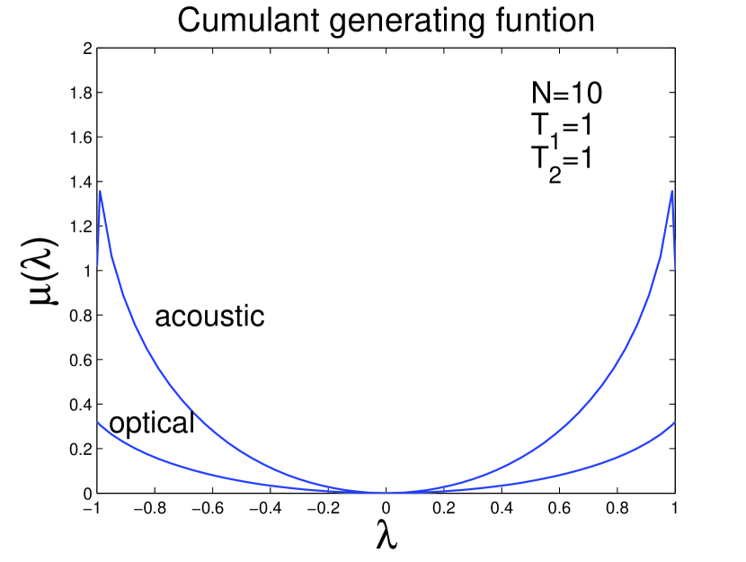
Figure 4: We depict the contributions to the cumulant generating function from the acoustic phonons, upper branch, and the optical phonons, the lower branch, as function of $\lambda$, based on the expression (52). We set $N=10$ and $T_{1}=T_{2}=1$, yielding a symmetrical CGF. The branch points are at $\lambda_{\pm}=\pm 1$.

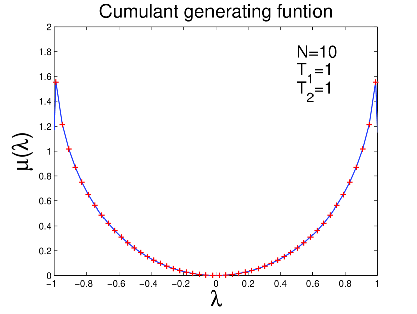
Figure 5: We depict the full cumulant generating function, $\mu$, including both the acoustic and optical contributions, given by (52) . Superimposed, indicated by red crosses, we have plotted the large $N$ approximation of CGF, $\tilde{\mu}$, given by (69). We have set $N=10$, $T_{1}=1$, and $T_{2}=1$. We find excellent agreement.

Based on the finite $N$ expression for the CGF in (52) we have in Fig. 4 plotted the contributions to the CGF arising from the acoustic and optical phonons, respectively, for $N=10$, $T_{1}=1$, and $T_{2}=1$. In this case the CGF is symmetrical. We note that the CGF is a downward convex function passing through the origin with branch points at $\lambda_{\pm}=\pm 1$. For $T_{1}\neq T_{2}$ the CGF is shifted and will pass through the origin for $\lambda=0$ and $\lambda=1/T_{1}-1/T_{2}$, consistent with the AFT in (1). In Fig. 5 we have superimposed a plot of of the $N\rightarrow\infty$ expression for the CGF, $\tilde{\mu}$, on a plot of $\mu$ for $N=10$ and $T_{1}=T_{2}=1$. We obtain an excellent fit indicating that the asymptotic large $N$ regime is attained already for small values of $N$.

VI.2 Transmission matrix

The transmission matrix $T^{\text{A},\text{B}}$ given by (51) is an essential ingredient in the evaluation of the CGF. Owing to the resonance structure in $G_{1N}^{\text{A,B}}$ the transmission matrix exhibits an oscillatory structure with period of order $1/N$. The maximum value and lower envelope is given by (66) and (67), respectively. In the large $N$ limit the oscillations merge together and allows for the smooth large $N$ approxiation implemented in Sec. V. Further analysis shows that in case B (odd), where the $u$ sublattice is driven by the heat reservoirs and the motion of $w$ sublattice is slaved to the motion of the $u$ sublattice, see Fig. 1, $T^{\text{B}}_{\text{max}}(\omega)=1$ for all $\omega$. In case A (even) the transmission matrix $T^{\text{A}}(\omega)$ exhibits a similar form except for a shift of the oscillatory pattern owing to the altered boundary conditions. Here the heat reservoirs drive each sublattice and only for the acoustic part do we have $T^{\text{A}}_{\text{max}}(\omega)=1$.

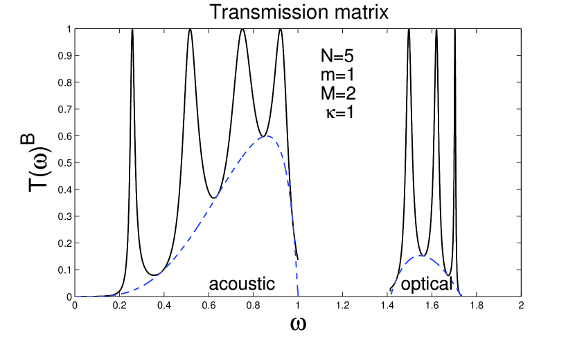
Figure 6: We depict the transmission matrix $T^{\text{B}}(\omega)$, given by (51), as function of $\omega$ for $N=5$, $m=1$, $M=2$, and $\kappa=1$ in the case B (odd). The oscillatory structure arises from the resonance structure in $D^{\text{B}}(\omega)$. The dashed line envelope arises from a large $N$ approximation derived in appendix. The upper bound is $T^{\text{B}}(\omega)=1$.

In Fig. 6 we have depicted $T^{\text{B}}(\omega)$ as a function of $\omega$ for $N=5$, $m=1$, $M=2$, and $\kappa=1$. The plot clearly shows the gap between the acoustic and optical phonons, the oscillatory structure being due to the resonance structure in $D^{\text{B}}(\omega)$. We have also plotted the lower envelope. Finally we notice that $T^{\text{B}}(\omega)$ is bounded from above by unity.

VI.3 Large deviation function

Here we briefly discuss some of the implication for the large deviation function. Inserting the expression for the characteristic heat function (2) in (18) we obtain at long times the following expression for the heat distribution.

$$P(Q,t)\sim\int_{-i\infty}^{i\infty}\frac{d\lambda}{2\pi i}\exp(-\lambda Q)\exp(t\mu(\lambda)).$$ (70)

This expression can be analyzed either as a Laplace transform or by a numerical simulation, see Fogedby and Imparato (2012). We shall not pursue such an approach here but note that a standard steepest descent argument or a Legendre transform Touchette (2009) implies that $P(Q,t)$ has the long time scaling form

$$P(Q,t)\sim\exp(tF(Q/t)),$$ (71)

where the large deviation function $F(Q/t)$ (LDF) is determined by

$$F(Q/t)=\mu(\lambda^{\ast})-\lambda^{\ast}\mu^{\prime}(\lambda^{\ast}).$$ (72)

Here $\lambda^{\ast}$ is determined by the saddle point condition

$$\mu^{\prime}(\lambda^{\ast})=Q/t.$$ (73)

For the LDF the AFT for $\mu(\lambda)$ in (1) implies

$$F(Q/t)-F(-Q/t)=-(Q/t)(\beta_{1}-\beta_{2}).$$ (74)

By inspection of the general expression (49) for the CGF we infer that $\mu(\lambda)$ has the form of a downward convex function passing through the origin $\mu(0)=0$ due to normalization and through $\mu(\beta_{1}-\beta_{2})=0$ owing to the fluctuation theorem. The branch points $\lambda_{\pm}$ are determined by the condition $1+T^{\text{A,B}}(\omega)f(\lambda)=0$, i.e., , the point where the log diverges. Since $T^{\text{A,B}}(\omega)\leq 1$, a little analysis shows that the branch point are given by

$$\lambda_{+}=\beta_{1},$$ (75)

$$\lambda_{-}=-\beta_{2}.$$ (76)

Deforming the contour in the integral (70) to pass along the real axis we pick up branch cut contributions in $\mu(\lambda)$. Heuristically, we conclude that for large $|Q/t|$ the LDF depends linearly on $Q/t$, i.e.,

$$F(Q/t)\sim-\lambda_{+}Q/t,~{}~{}~{}~{}\text{for}~{}Q/t\gg 0~{},$$ (77)

$$F(Q/t)\sim-|\lambda_{-}||Q/t|,~{}\text{for}~{}Q/t\ll 0;$$ (78)

where $\lambda_{+}$ and $\lambda_{-}$ have been defined above. The heat distribution thus exhibits exponential tails for large $|Q/t|$, i.e.,

$$P(Q/t)\propto\exp(-\lambda_{+}Q)~{}\text{for}~{}Q/t\gg 0,$$ (79)

$$P(Q/t))\propto\exp(-|\lambda_{-}||Q|)~{}\text{for}~{}Q/t\ll 0,$$ (80)

with $\lambda_{+}$ and $\lambda_{-}$ given by (75) and (76). It is interesting that the tails in the $Q$ distribution are determined only by the reservoir temperatures.

VII Conclusion

In the present paper we have extended our previous work on the cumulant generating function and the large deviation function for the simple harmonic chain to the case of an alternating mass chain. From a technical point of view the analysis is more complex due to the two band structure arising from the acoustic and optical phonon branches. We find that the transmission matrix exhibits a two band structure. These results are in complete agreement with Kannan el al Kannan et al. (2012). The contributions from the two branches to the cumulant generating function are also identified. Finally, we have extended the large $N$ approximation in Fogedby and Imparato (2012). We find that the cumulant generating function and thus the heat and higher cumulants of the heat are manifestly independent of the system size $N$ for large $N$. We find that the independence of $N$ sets in already at small $N$. This is consistent with the fact that the system does not attain local equilibrium and that Fourier’s law does not hold. Finally, we have confirmed that the results depend on whether the chain is composed of an even (case A) or odd (case B) number of particles.

Appendix: Green’s functions

A basic ingredient in our analysis are the Green’s functions $G$ and $F$ in (39) and (40) describing the propagation of lattice vibrations across the chain. In Kannan et al. Kannan et al. (2012) the derivation of the Green’s functions is done using a determinantal approach, here we derive them directly from the equations of motion (23) and (24) together with (35) to (38). The scheme follows the method used in Fogedby and Imparato (2012) with the added complications due to the two band structure. We obtain for the $u$ and $w$ sub lattices in the asymmetrical case A, see Fig. 1, the equations of motion

$$\Omega_{\text{A}}u_{1}=\kappa_{\text{A}}u_{2}+\xi_{1},$$ (81)

$$\Omega_{\text{C}}u_{N}=\kappa_{\text{D}}u_{N-1}+\xi_{N},$$ (82)

$$\Omega_{\text{D}}w_{1}=\kappa_{\text{C}}w_{2}+\xi_{1},$$ (83)

$$\Omega_{\text{B}}w_{N}=\kappa_{\text{B}}w_{N-1}+\xi_{N}.$$ (84)

Likewise, in the symmetrical case B, see see Fig. 1, the equations of motion

$$\Omega_{\text{A}}u_{1}=\kappa_{\text{A}}u_{2}+\xi_{1},$$ (85)

$$\Omega_{\text{A}}u_{N+1}=\kappa_{\text{A}}u_{N}+\xi_{N},$$ (86)

$$\Omega_{\text{D}}w_{1}=\kappa_{\text{C}}w_{2}+\xi_{1},$$ (87)

$$\Omega_{\text{D}}w_{N}=\kappa_{\text{C}}w_{N-1}+\xi_{N}.$$ (88)

We have introduced the parameters

$$\Omega_{\text{A}}=\Omega_{1}-\kappa^{2}/\tilde{\Omega}_{2},$$ (89)

$$\Omega_{\text{B}}=\Omega_{2}-\kappa^{2}/\tilde{\Omega}_{1},$$ (90)

$$\Omega_{\text{C}}=(\Omega_{2}/\kappa)(\tilde{\Omega}_{1}-\kappa^{2}/\tilde{\Omega}_{2})-\kappa,$$ (91)

$$\Omega_{\text{D}}=(\Omega_{1}/\kappa)(\tilde{\Omega}_{2}-\kappa^{2}/\tilde{\Omega}_{1})-\kappa,$$ (92)

$$\kappa_{\text{A}}=\kappa^{2}/\tilde{\Omega}_{2},$$ (93)

$$\kappa_{\text{B}}=\kappa^{2}/\tilde{\Omega}_{1},$$ (94)

$$\kappa_{\text{C}}=\kappa\Omega_{1}/\tilde{\Omega}_{1},$$ (95)

$$\kappa_{\text{D}}=\kappa\Omega_{2}/\tilde{\Omega}_{2},$$ (96)

where $\tilde{\Omega}_{1}$, $\tilde{\Omega}_{2}$, $\Omega_{1}$, and $\Omega_{2}$ are given by (21), (22), (33), and (34). Note that unlike the simple harmonic chain the parameters here acquire an explicit $\omega$ dependence due to the dynamical coupling of the two sub lattices.

Searching for plane wave solutions of the form

$$u_{n}=\alpha_{1}\exp(ipn)+\beta_{1}\exp(-ipn),$$ (97)

$$w_{n}=\alpha_{2}\exp(ipn)+\beta_{2}\exp(-ipn),$$ (98)

the coefficients $\alpha$ and $\beta$ are readily determined by insertion in the equations of motion.

Case A:

$$G_{n1}^{\text{A}}=\frac{\Omega_{\text{C}}\sin(N-n)p-\kappa_{\text{D}}\sin(N-1-n)p}{D_{1}^{\text{A}}},$$ (99)

$$G_{nN}^{\text{A}}=\frac{\Omega_{\text{A}}\sin(n-1)p-\kappa_{\text{A}}\sin(n-2)p}{D_{1}^{\text{A}}},$$ (100)

$$F_{n1}^{\text{A}}=\frac{\Omega_{\text{B}}\sin(N-n)p-\kappa_{\text{B}}\sin(N-1-n)p}{D_{2}^{\text{A}}},$$ (101)

$$F_{nN}^{\text{A}}=\frac{\Omega_{\text{D}}\sin(n-1)p-\kappa_{\text{C}}\sin(n-2)p}{D_{2}^{\text{A}}},$$ (102)

$$D_{1}^{\text{A}}=\Omega_{\text{A}}\Omega_{\text{C}}\sin(N-1)p-(\Omega_{\text{A}}\kappa_{\text{D}}+\Omega_{\text{C}}\kappa_{\text{A}})\sin(N-2)p+\kappa_{\text{A}}\kappa_{\text{D}}\sin(N-3)p,$$ (103)

$$D_{2}^{\text{A}}=\Omega_{\text{B}}\Omega_{\text{D}}\sin(N-1)p-(\Omega_{\text{D}}\kappa_{\text{B}}+\Omega_{\text{B}}\kappa_{\text{C}})\sin(N-2)p+\kappa_{\text{B}}\kappa_{\text{C}}\sin(N-3)p.$$ (104)

Case B:

$$G_{n1}^{\text{B}}=\frac{\Omega_{\text{A}}\sin(N-n)p-\kappa_{\text{A}}\sin(N-1-n)p}{D_{1}^{\text{B}}},$$ (105)

$$G_{nN}^{\text{B}}=\frac{\Omega_{\text{A}}\sin(n-1)p-\kappa_{\text{A}}\sin(n-2)p}{D_{1}^{\text{B}}},$$ (106)

$$F_{n1}^{\text{B}}=\frac{\Omega_{\text{D}}\sin(N-n)p-\kappa_{\text{C}}\sin(N-1-n)p}{D_{2}^{\text{B}}},$$ (107)

$$F_{nN}^{\text{B}}=\frac{\Omega_{\text{D}}\sin(n-1)p-\kappa_{\text{C}}\sin(n-2)p}{D_{2}^{\text{B}}},$$ (108)

$$D_{1}^{\text{B}}=\Omega_{\text{A}}^{2}\sin(N-1)p-2\Omega_{\text{A}}\kappa_{\text{A}}\sin(N-2)p+\kappa_{\text{A}}^{2}\sin(N-3)p,$$ (109)

$$D_{2}^{\text{B}}=\Omega_{\text{D}}^{2}\sin(N-1)p-2\Omega_{\text{D}}\kappa_{\text{C}}\sin(N-2)p+\kappa_{\text{C}}^{2}\sin(N-3)p.$$ (110)

We have in particular

$$G_{1N}^{\text{A}}=\frac{\kappa_{\text{A}}\sin p}{D_{1}^{\text{A}}},$$ (111)

$$G_{1N}^{\text{B}}=\frac{\kappa_{\text{A}}\sin p}{D_{1}^{\text{B}}},$$ (112)

Detailed inspection of the above results for $G$ and $F$ shows that they are in agreement with the determinantal results in Kannan et al. (2012).

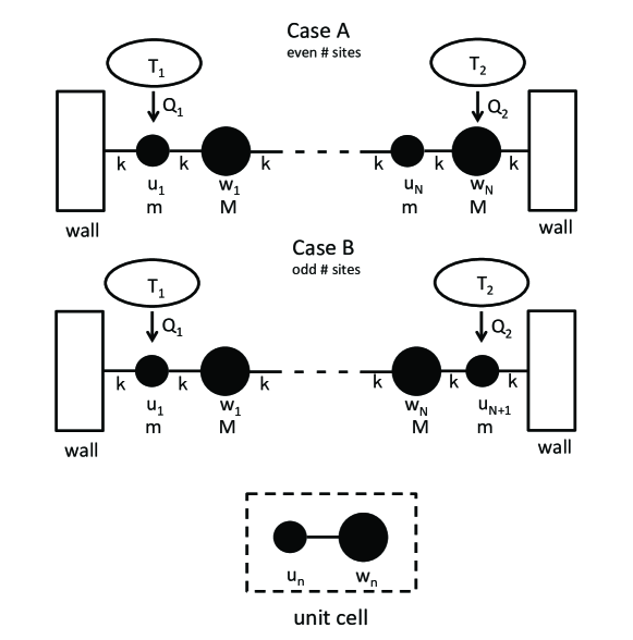
Figure 1: We depict the two possible configuration for the alternating mass chain and the appropriate unit cell with basis. In case A we have an integer set of unit cells, each containing a mass $m$ particle with displacement $u_{n}$ and a mass $M$ particle with displacement $w_{n}$. The particles are attached by springs with spring constant $\kappa$. Particle $u_{1}$ is driven by a reservoir at temperature $T_{1}$; particle $w_{n}$ driven at $T_{2}$. In case B particle $u_{N+1}$ in a half filled unit cell is driven at $T_{2}$.

References

- Trepagnier et al. (2004) E. Trepagnier, C. Jarzynski, F. Ritort, G. Crooks, C. Bustamante, and J. Liphardt, Proc. Natl. Acad. Sci. USA 101, 15038 (2004).
- Collin et al. (2005) D. Collin, F. Ritort, C. Jarzynski, S. B. Smith, I. T. Jr, and C. Bustamante, Nature 437, 231 (2005).
- Tietz et al. (2006) C. Tietz, S. Schuler, T. Speck, U. Seifert, and J. Wrachtrup, Phys. Rev. Lett. 97, 050602 (2006).
- Blickle et al. (2006) V. Blickle, T. Speck, L. Helden, U.Seifert, and C. Bechinger, Phys. Rev. Lett. 96, 070603 (2006).
- Wang et al. (2002) G. Wang, E. Sevick, E. Mittag, D. J. Searles, and D. J. Evans, Phys. Rev. Lett. 89, 050601 (2002).
- Imparato et al. (2007) A. Imparato, L. Peliti, G. Pesce, G. Rusciano, and A. Sasso, Phys. Rev. E 76, 050101R (2007).
- Douarche et al. (2006) F. Douarche, S. Joubaud, N. B. Garnier, A. Petrosyan, and S. Ciliberto, Phys. Rev. Lett. 97, 140603 (2006).
- Garnier and Ciliberto (2007) N. Garnier and S. Ciliberto, Phys. Rev. E 71, 060101(R) (2007).
- Imparato et al. (2008) A. Imparato, P. Jop, A. Petrosyan, and S. Ciliberto, J. Stat. Mech p. P10017 (2008).
- Jarzynski (1997) C. Jarzynski, Phys. Rev. Lett. 78, 2690 (1997).
- Kurchan (1998) J. Kurchan, J. Phys. A 31, 3719 (1998).
- Gallavotti (1996) G. Gallavotti, Phys. Rev. Lett. 77, 4334 (1996).
- Crooks (1999) G. E. Crooks, Phys. Rev. E 60, 2721 (1999).
- Crooks (2000) G. E. Crooks, Phys. Rev. E 61, 2361 (2000).
- Seifert (2005a) U. Seifert, Phys. Rev. Lett. 95, 040602 (2005a).
- Seifert (2005b) U. Seifert, Europhys. Lett 70, 36 (2005b).
- Evans et al. (1993) D. J. Evans, E. G. D. Cohen, and G. P. Morriss, Phys. Rev. Lett. 71, 2401 (1993).
- Evans and Searles (1994) D. J. Evans and D. J. Searles, Phys. Rev. E 50, 1645 (1994).
- Gallavotti and Cohen (1995) G. Gallavotti and E. G. D. Cohen, Phys. Rev. Lett. 74, 2694 (1995).
- Lebowitz and Spohn (1999) J. L. Lebowitz and H. Spohn, J. Stat. Phys. 95, 333 (1999).
- Gaspard (2004) P. Gaspard, J. Stat. Phys. 117, 599 (2004).
- Imparato and Peliti (2006) A. Imparato and L. Peliti, Phys. Rev. E 74, 026106 (2006).
- van Zon and Cohen (2003a) R. van Zon and E. G. D. Cohen, Phys. Rev. Lett. 91, 110601 (2003a).
- van Zon et al. (2004) R. van Zon, S. Ciliberto, and E. G. D. Cohen, Phys. Rev. Lett. 92, 130601 (2004).
- van Zon and Cohen (2003b) R. van Zon and E. G. D. Cohen, Phys. Rev. 67, 046102 (2003b).
- van Zon and Cohen (2004) R. van Zon and E. G. D. Cohen, Phys. Rev. E 69, 056121 (2004).
- Speck and Seifert (2005) T. Speck and U. Seifert, Eur. Phys. J. B 43, 521 (2005).
- Saito and Dhar (2007) K. Saito and A. Dhar, Phys. Rev. Lett. 99, 180601 (2007).
- Kundu et al. (2011) A. Kundu, S. Sabhapandit, and A. Dhar, J. Stat. Mech. p. P03007 (2011).
- Sabhapandit (2011) S. Sabhapandit, Europhys. Lett 96, 20005 (2011).
- Sabhapandit (2012) S. Sabhapandit, Phys. Rev. E 85, 021108 (2012).
- Fogedby and Imparato (2012) H. C. Fogedby and A. Imparato, J. Stat. Mech. p. P04005 (2012).
- Bonetto et al. (2000) F. Bonetto, J. L. Lebowitz, and L. Rey-Bellet, Math. Phys. 2000, 128-150 (2000).
- Ashcroft and Mermin (1976) N. W. Ashcroft and N. D. Mermin, Solid State Physics (Holt, Rinehart and Winston, New York, 1976).
- Kannan et al. (2012) V. Kannan, A. Dhar, and J. L. Lebowitz, Phys. Rev. E 85, 041118 (2012).
- Casher and Lebowitz (1971) A. Casher and J. L. Lebowitz, J. Math. Phys. 12, 1701 (1971).
- O’Connor and Lebowitz (1974) A. J. O’Connor and J. L. Lebowitz, J. Math. Phys. 15, 692 (1974).
- Rieder et al. (1967) Z. Rieder, J. L. Lebowitz, and E. Lieb, J. Math. Phys. 8, 1073 (1967).
- Nakazawa (1970) H. Nakazawa, Prog. Theo. Phys. (Suppl.) 45, 231 (1970).
- Gradshteyn and Ryzhik (1965) I. S. Gradshteyn and I. M. Ryzhik, Table of Integrals. Series, and Products (Academic Press, New York, 1965).
- Touchette (2009) H. Touchette, Phys. Rep. 478, 1 (2009).
- den Hollander (2000) F. den Hollander, Large Deviations, vol. 14 (American Mathematical Society, Providence, R.I., 2000).
- Roy and Dhar (2008) D. Roy and A. Dhar, J. Stat. Phys. 131, 535 (2008).