Tracking via Motion Estimation with Physically Motivated Inter-Region Constraints

Abstract

In this paper, we propose a method for tracking structures (e.g., ventricles and myocardium) in cardiac images (e.g., magnetic resonance) by propagating forward in time a previous estimate of the structures via a new deformation estimation scheme that is motivated by physical constraints of fluid motion. The method employs within structure motion estimation (so that differing motions among different structures are not mixed) while simultaneously satisfying the physical constraint in fluid motion that at the interface between a fluid and a medium, the normal component of the fluid’s motion must match the normal component of the motion of the medium. We show how to estimate the motion according to the previous considerations in a variational framework, and in particular, show that these conditions lead to PDEs with boundary conditions at the interface that resemble Robin boundary conditions and induce coupling between structures. We illustrate the use of this motion estimation scheme in propagating a segmentation across frames and show that it leads to more accurate segmentation than traditional motion estimation that does not make use of physical constraints. Further, the method is naturally suited to interactive segmentation methods, which are prominently used in practice in commercial applications for cardiac analysis, where typically a segmentation from the previous frame is used to predict a segmentation in the next frame. We show that our propagation scheme reduces the amount of user interaction by predicting more accurate segmentations than commonly used and recent interactive commercial techniques.

I Introduction

Accurate boundary detection of deforming structures from time-varying medical images (e.g., cardiac MRI) is an important step in many clinical applications that study structure and function of organs non-invasively. While many methods have been proposed to determine the boundary of a deforming structure by segmenting each frame based on image intensity statistics and incorporating training data (see Section I-A), it is sometimes easier to exploit the temporal coherence of the structure, and apply a tracking framework. That is, one matches a current estimate of the structure of interest at time $t$ to the image at time $t+1$ to detect the organ at time $t+1$. This requires an accurate registration between images.

A difficulty in registration stems from the aperture problem - many different registrations are able to explain two images, and therefore, regularization is needed to constrain the set of possible solutions. Typically, global regularization is used. However, the image consists of many structures, each moving with different motions/deformations, and global regularization implies that smoothing is performed across multiple structures. Therefore, motion/deformation information from surrounding structures is used in the registration estimate within the structure of interest; this leads to errors in the registration and in the structure segmentation.

In this work, we derive a registration method that estimates motion separately in each structure by performing only within structure regularization (so that motions from heterogeneous structures are not mixed) while satisfying physical motion constraints (from fluid mechanics) across the boundary between two structures. Specifically, the physical constraint is that the motion of a fluid in a medium at the interface is such that the normal components of the motions are the same. We derive a motion estimation scheme that incorporates these physical considerations. We use our new motion estimation scheme in a tracking algorithm to segment structures. That is, given the initial segmentation in the first frame, our algorithm automatically propagates the segmentation to the next frame. Although our methodology is not restricted to a particular imaging modality or a particular structure, we focus on a prominent application where the physically motivated considerations are natural - segmenting the left (LV), right ventricle (RV), and the surrounding heart muscle from cardiac MRI. We demonstrate that our new motion estimation scheme leads to more accurate segmentation of the LV and RV than using traditional global regularization.

Further, the main motivation for our new motion estimation scheme is segmentation propagation in interactive segmentation of image sequences. Segmentation propagation is a basic step to predict the segmentation in the next frame from the current frame in interactive methods. Interactive approaches are still the norm in commercial medical applications (particularly cardiac MRI) as fully automated segmentation (see discussion in Section I-A) is still at the research stage. An accurate segmentation propagation reduces the amount of interaction for the user. We show that our propagation scheme, with physically viable motion, leads to better segmentation propagation than recent existing commercially available software for cardiac segmentation, and would thus require less interaction.

I-A Related Work: Cardiac Segmentation

We now give a brief review of the cardiac image segmentation literature, which places our work in appropriate context. For a more thorough review of literature, we direct the reader to recent review articles [35, 53].

Early methods for automatic segmentation of cardiac images involve the use of image partitioning algorithms (e.g., active contours [19] implemented via level sets [31], graph cuts [3], or convex optimization methods [4]), which optimize energies that integrate basic image features such as edges [36], intensity statistics [8], motion cues [11], and basic smoothness priors of the partition. These methods are good at partitioning the image into regions of homogeneous statistics, however, the regions of the partition do not typically select regions that correspond to physical objects/structures (e.g., the left/right ventricle, or the myocardium). Therefore, there have been two approaches to augment basic segmentation algorithms to determine object boundaries: training-based approaches where manually segmented objects from training images are used to construct a model which is then used in automatic segmentation, and the second approach is interactive approaches where human interaction is used to correct errors from basic segmentation approaches.

Since our contribution lies in reducing the amount of interaction required in interactive approaches, we give only a brief review of training based approaches next before moving to review interactive approaches. In training-based approaches, training data is used to construct a model of the heart. Early approaches constructed models of the heart manually by using simple geometric approximations of the heart made by observing training images, e.g., a generic model of the heart constructed from truncated ellipses [43] that are used to model the ventricles. More specific models for the heart tailored to the training data use the training data of manually segmented organs more directly. Some approaches (e.g., [45, 47, 22, 16, 54, 50, 51]) make use of active shape and appearance models [7, 6] where manual landmarks around the boundary of the object in training images model the shape, and texture descriptors describing a neighborhood around the landmark are used to model object appearance. Such landmarks and descriptors allow for natural use of PCA to generate a statistical model. More precise models of shape are based on performing PCA of segmented objects using mesh-based approaches [13] or geometric level set representations [46, 34]. The previous methods construct static models of the heart, however, the heart is a dynamic object, and thus, dynamic models of shape [39, 52] are constructed by considering the shape from multiple frames in the sequence as a time-varying object. Once the heart model is constructed from training data, to perform object segmentation of an image, the model must be fitted to the image. This can be done in a number of ways, the most common method for shape models (e.g. [5, 10, 46]) is to restrict the optimization of the energies based on basic image features (discussed in the previous paragraph) to the shapes determined by the parametric shape model. Other approaches that have both shape and appearance information deform the average shape/appearance, i.e., the atlas, via registration to fit the target image, thereby determining the object segmentation [26, 54, 18, 21].

Although a fully automatic solution to segmentation of the heart (as in the methods above) and its sub-structures is the ideal goal, these methods are not accurate enough (especially when there is deviation from the training set, e.g., in cases of disease) to be used in many cardiac applications (e.g., [53, 23, 33, 46, 20, 42, 27, 24, 47, 28]). Therefore, in practical commercial applications, interactive approaches to segmentation in which a user corrects the prediction of automatic segmentation are still the norm. Various techniques in the computer vision community (e.g., [49, 2, 9]) have been designed to incorporate interaction in the form of seed points (belonging to the object and the background). These methods modify energies based on simple image features (discussed in the first paragraph) to incorporate constraints from the seed points entered by the user. Other interactive methods allow for a manual or semi-automated segmentation of the first frame in the cardiac sequence and then attempt to propagate the segmentation to sub-sequent frames, thereby predicting a segmentation that needs little interaction to correct [41, 30]. Several methods exist to propagate the initial segmentation (e.g., by registration [41, 30]) and/or by using the manual segmentation in the first frame as initialization to an automated segmentation algorithm. Several commercial softwares for interactive heart segmentation have been designed. For example, the recent software Medviso [15, 44] allows the user to input an initial segmentation, which is then propagated to subsequent frames in order to segment various structures including the ventricles and myocardium. The software also allows for various other manual interactions to correct any errors in the propagation. The algorithm is a culmination of many techniques including registration to propagate the segmentation as well as the use of automated methods training data to encode shape priors.

I-B Related Work: Registration

The goal of our method is to improve the propagation method in interactive techniques so that less interaction is required by the user. We do so by deriving a registration technique that better models the underlying physics of the motion of ventricles and myocardium, in particular constraints formed from interactions between adjacent regions (e.g., ventricles and the surrounding muscle). Since our works relates to registration, we give a brief review of recent related work in registration.

The goal of registration is to find pixel-wise correspondence between two images in a sequence. The difficulty arises from the aperture ambiguity: there are infinitely many transformations that map one image to the other, and thus regularization must be used to constrain the solution. The pioneering work [17] from the computer vision literature uses a uniform global smoothness penalty to estimate the registration under small pixel displacements. Larger deformations with global regularization that lead to diffeomorphic registrations, a property of a proper registration in typical medical images, has been considered by [1, 48]. For cardiac images (as well as other medical images), there are multiple objects (sub-structures) that each have different motion characteristics, thus global regularization across adjacent objects (mixing heterogenous motion characteristics) is not desired, and moreover, there are physical constraints between adjacent regions that a registration based on global regularization does not satisfy. In particular, in cardiac applications (and others), the ventricles and the heart muscle (myocardium), both mostly fluids, are such that the normal component on the boundary of the motions (velocity) of both structures are equal. The previous constraint is from the fact that the ventricle and the surrounding muscle do not separate during motion. Further, the No-Slip condition [29] from fluid mechanics for viscous fluids states that the motion of the fluid relative to the boundary (the tangent component) is zero. The scale at which this happens is small compared with the resolution of the imaging device, and thus we allow the tangent components to be arbitrary across the boundary, although our technique can easily be modified if the No-Slip condition is desired to be enforced.

There has been recent work in the medical imaging literature that has considered other forms of regularization rather than global regularization. Indeed, in the case of lung registration, the lung slides along the rib-cage, and the motion of both these structures are different and thus global regularization is not desired. In [32, 40] an anisotropic global regularization is used to favor smoothing in the tangential direction near organ boundaries. In [38], Log-Demons [48] is generalized so that smoothing is performed on the tangent component of the registration within organs, and the normal component is globally smoothed on the whole image. Our approach differs from these works in that our technique is motivated by the physical constraints of fluid motion present in the heart. Further, in our method, regularization is only performed within homogeneous structures (different than [38] which smoothes the normal component across structures, mixing inhomeogeneous motions), and smoothing along the tangential direction of the boundary in [32, 40] does not necessarily ensure that the normal motions equality on the boundary. While [38] achieves equal normal motions, it does so by smoothing across tstructures.

I-C Organization of Paper

In Section II, we specify the motion and registration model between frames in an image sequence, in particular, the motion constraint between structures. In Section III, we use the motion model to setup a variational problem for estimating the motion given the two images assuming infinitesimal motion, and then show how to estimate the motion using two different methods. In Section III, we show how to estimate non-infinitesimal motion that are typical between frames and simultaneously propagate the segmentation from the previous frame to the next frame. Finally, we in Section V show a series of experiments to verify our method as well as compare it to an existing recent commercial software package for interactive cardiac segmentation.

II Motion and Registration Model

In this section, we state the assumptions that we use to derive our method for piecewise registration whose normal component is continuous across organ boundaries. We assume the standard brightness constancy plus noise model:

$$J_{1}(x)=J_{0}(w^{-1}(x))+\eta(x),\,x\in\Omega$$ (1)

where $\Omega\subset\mathbb{R}^{n}$ ($n=2,3$) is the image domain, $J_{0},J_{1}:\Omega\to\mathbb{R}$ are the images sampled from the time-varying imagery at two consecutive times, $w:\Omega\to\Omega$ is the registration between frames $J_{0}$ and $J_{1}$, and $\eta$ is a noise process. The structure of interest in $J_{0}$ is denoted $R\subset\Omega$ and the background is denoted $\Omega\backslash R$. Our model can be extended to any number of organs, but we forgo the details for simplicity of presentation. The structure in frame $J_{1}$ is then assumed to be $w(R)$.

The registration is an invertible map, and thus we represent it as an integration of a time varying infinitesimal velocity field (following standard representation in the fluid mechanics literature):

$$w(x)=\phi_{T}(x),\,\phi_{s}(x)=x+\int_{0}^{s}v_{\tau}(\phi_{\tau}(x))\,\mathrm{d}\tau,\,s\in[0,T]$$ (2)

where $T>0$, $v_{\tau}:\Omega\to\mathbb{R}^{n}$ is a velocity field, and $\phi_{\tau}:\Omega\to\Omega$ for every $\tau\in[0,T]$. The map $\phi_{\tau}$ is such that $\phi_{\tau}(x)$ indicates the mapping of $x$ after it flows along the velocity field for time $\tau$, which is an artificial time parameter.

We assume that the motion/deformation of the structure of interest $R$ and the surrounding region have different characteristics and therefore the registration $w$ consists of two components (one can easily extend to more components, but we use only two for simplicity of notation), $w^{in}$ and $w^{out}$ defined inside the organ of interest $R$ and outside the organ $\Omega\backslash R$, resp. This can be achieved with a velocity field that has two components $v^{in}_{\tau},v^{out}_{\tau}$ (both smooth within their domains):

$$w(x)=\begin{cases}w^{in}(x)&x\in R\\ w^{out}(x)&x\in\Omega\backslash R\end{cases},\quad v_{\tau}(x)=\begin{cases}v^{in}_{\tau}(x)&x\in R_{\tau}\\ v^{out}_{\tau}(x)&x\in\Omega\backslash R_{\tau}\end{cases},$$ (3)

where $R_{\tau}=\phi_{\tau}(R)$. This implies that $w^{in}$ and $w^{out}$ are smooth and invertible. When the structure $R$ contains a fluid (as in the ventricles) and $\Omega\backslash R$ is the surrounding medium (e.g., myocardium), the normal as in our case of interest, there is a physical constraint from fluid mechanics imposed on $v^{in}_{\tau}$ and $v^{out}_{\tau}$ at the boundary $\partial R_{\tau}$. The constraint is that the normal component of $v^{in}_{\tau}$ and $v^{out}_{\tau}$ are equal on $\partial R_{\tau}$:

$$v^{in}_{\tau}(x)\cdot N(x)=v^{out}_{\tau}(x)\cdot N(x),\,x\in\partial R_{\tau},$$ (4)

where $N$ indicates the surface normal of $\partial R_{\tau}$. The condition implies that the two mediums $R$ and $\Omega\backslash R$ do not separate when deformed by the infinitesimal motion. Further, the No-Slip Condition from fluid mechanics [29] implies that the motion of the fluid relative to the surrounding medium is zero at the interface, thus, the tangent components of $v^{in}_{\tau}$ is zero. However, the scale at which the tangential component is approximately zero may be at a scale much smaller than determined by the resolution of the imaging device. Therefore, we do not enforce this constraint, although if desired, the constraint can easily be incorporated in our framework in the next section.

Modeling the velocity with two separate components allows for different deformation for the structure of interest and surrounding medium, and the constraint (4) couples the two components of velocity, in a physically plausible manner. This implies continuity of the normal component of $v_{\tau}$ across $\partial R_{\tau}$, but not necessarily differentiability, as dictated by materials of different chemical composition.

III Energy-Based Formulation for Infinitesimal Deformations

In this section, we consider the case when the registration can be approximated as $w(x)=x+v(x)$ where $v$ is an infinitesimal deformation, and we show how one computes $v$ such that (4) is satisfied while applying regularization only within regions and not across regions.

We design an optimization problem so that the solution determines the infinitesimal deformation $v$ of interest. In a tracking framework, $R$ is given (e.g., at the initial frame or the previous estimate from a previous frame), and the goal is to determine $v$ and then $R+v=\{x+v(x)\,:\,x\in\Omega\}$ is the object in the next frame (assuming the deformation between frames is small). The energy that we consider is

$$E(v_{i},v_{o};R,I) =\frac{1}{2}\int_{R}\left(|J_{1}-I+\nabla I\cdot v_{i}|^{2}+\alpha_{i}|\nabla v_{i}|^{2}\right)\,\mathrm{d}x+\frac{1}{2}\int_{\Omega\backslash R}\left(|J_{1}-I+\nabla I\cdot v_{o}|^{2}+\alpha_{o}|\nabla v_{o}|^{2}\right)\,\mathrm{d}x$$ (5)

subject to $$v_{i}\cdot N=v_{o}\cdot N\mbox{ on }\partial R$$ (6)

The infinitesimal deformations are defined $v_{i}:R\to\mathbb{R}^{n}$ and $v_{o}:\Omega\backslash R\to\mathbb{R}^{n}$ (as in (3)). The operator $\nabla$ is the spatial gradient defined within $R$ or $\Omega\backslash R$ (without crossing $\partial R$). Note that the first term in each of the above integrals arises from a linearization of (1) (when $I=J_{0}$), and due to the well-known aperture problem, regularization (the second term in each of the integrals) is required to invert (3). It should be emphasized that the regularization is done separately within each of the regions. The weights $\alpha_{i},\alpha_{o}>0$ indicate the amount of regularity desired within each region.

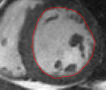
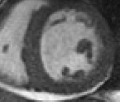
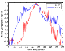
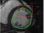
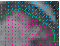
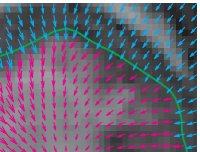
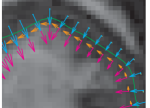
The problem above is a generalization of Horn & Schunck optical flow. Note that solving for the Horn & Schunck optical flow within each region separately does not lead to motions such that at the interface, they have equal normal components (see Figure 1), whereas the solution of (5) to be presented in subsequent sections does. Note that computing Horn & Schunck optical flow in each region requires boundary conditions (and typically they are chosen to be Neumann boundary conditions: $\nabla v_{i}\cdot N=0$ and $\nabla v_{o}\cdot N=0$ on $\partial R$). Note that replacing these boundary conditions with the boundary constraint (6) does not specify a unique solution. Also, while Horn & Schunck optical flow computed on the whole domain $\Omega$ naturally gives a globally smooth motion, which by default satisfies matching normals at the interface, this is not natural for the ventricles / myocardium, where different motions exist in the regions (see Figure 2), and the motions should not be smoothed across the regions.

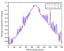
In the subsections below, we show how the matching normal constraint can be enforced approximately and exactly. This leads to PDEs for $v_{i}$ and $v_{o}$ that are coupled with boundary conditions that are not seen in optical flow estimation and medical image registration.

image + boundary	next image	within region optical flow	our method

Figure 1: Regularization within regions alone does not necessarily induce matching normal motions. [First]: $I_{1}$ with the boundary of $R$, $\partial R$, marked in red. [Second]: $I_{2}$. [Third]: Normal components of the velocities just inside and just outside $\partial R$ using traditional optical flow computation separately within $R$ and $\Omega\backslash R$. Notice that the normal components of the velocities inside and outside $\partial R$ are different, and therefore not physically viable. [Fourth]: The result of our approach using regularization only within regions, while satisfying the normal motion matching constraint: normal motions along $\partial R$ are equal.

image + boundary	global optical flow	our method	our method (motion decomp.)

Figure 2: Why regularization within regions and matching motion normals constraint? Heart is contracting. [First]: $J_{0}$, $\partial R$ in green, and the red box is zoomed in subsequent images. [Second]: velocity field with global regularization shows smoothing across the boundary. [Third]: velocity fields $v^{in},v^{out}$ with within region regularization and normal constraint shows clear difference to global regularization. [Fourth]: normal and tangent components of inside/outside velocities $v^{in},v^{out}$; notice the matching normal components, but discontinuity of tangent components across boundary (tangent component outside is nearly zero). Outside boundary velocity indicates contractive behavior of myocardium, and tangent component inside indicates some circulation near boundary: cannot be captured with globally smooth regularization.

III-A Energy Optimization with a Soft Constraint

The first approach to optimize (5) subject to (6) is to construct a new energy that includes a term that penalizes deviations away from (6). This greatly favors deformations that satisfy the constraint, but the optimization of the energy does not in general satisfy the constraint exactly. We consider the following energy:

$$E_{s}(v_{i},v_{o};R,I)=E(v_{i},v_{o};R,I)+\frac{\beta}{2}\int_{\partial R}(v_{i}\cdot N-v_{o}\cdot N)^{2}\,\mathrm{d}s$$ (7)

where $\beta>0$. Note that the space of $v_{i},v_{o}$ is a linear space, and the energy $E_{s}$ is convex and thus, any local optimum is a global optimum. To find the necessary conditions, we compute the first variation of $E_{s}$. Let $h_{i}:R\to\mathbb{R}^{2}$ and $h_{o}:\Omega\backslash R\to\mathbb{R}^{2}$ be perturbations of $v_{i}$ and $v_{o}$, then the first variation in $(h_{i},h_{o})$ (after simplification) is

$$dE(v_{i},v_{o})\cdot(h_{i},h_{o}) =\int_{R}\left[(J_{1}-I+\nabla I\cdot v_{i})\nabla I-\alpha_{i}\Delta v_{i}\right]\cdot h_{i}\,\mathrm{d}x$$ (8)

$$+\int_{\Omega\backslash R}\left[(J_{1}-I+\nabla I\cdot v_{o})\nabla I-\alpha_{o}\Delta v_{o}\right]\cdot h_{o}\,\mathrm{d}x$$ (9)

$$+\int_{\partial R}\left[\alpha_{i}(\nabla v_{i}\cdot N)+\beta(v_{i}\cdot N-v_{o}\cdot N)N\right]\cdot h_{i}\,\mathrm{d}s$$ (10)

$$+\int_{\partial R}\left[\alpha_{o}(\nabla v_{o}\cdot N)+\beta(v_{i}\cdot N-v_{o}\cdot N)N\right]\cdot h_{o}\,\mathrm{d}s$$ (11)

where the first two terms in the two boundary integrals are obtained from integration by parts, and $\Delta$ denotes the Laplacian operator. The necessary conditions for a minimum are obtained by choosing $v_{i},v_{o}$ such that $dE(v_{i},v_{o})\cdot(h_{i},h_{o})=0$ for all $h_{i},h_{o}$, and thus, we have

$$-\alpha_{i}\Delta v_{i}+\nabla I\nabla I^{T}v_{i} =-(J_{1}-I)\nabla I,\quad\mbox{in }R$$ (12)

$$-\alpha_{o}\Delta v_{o}+\nabla I\nabla I^{T}v_{o} =-(J_{1}-I)\nabla I,\quad\mbox{in }\Omega\backslash R$$ (13)

$$\alpha_{i}\nabla v_{i}\cdot N+\beta(v_{i}\cdot N-v_{o}\cdot N)N =0,\quad\mbox{on }\partial R$$ (14)

$$\alpha_{o}\nabla v_{o}\cdot N+\beta(v_{i}\cdot N-v_{o}\cdot N)N =0,\quad\mbox{on }\partial R$$ (15)

where ^T indicates transpose. The last two boundary conditions are Robin boundary conditions (these conditions are constraints on a linear combination of the normal derivatives of the functions and the function values on the boundary). These boundary conditions specify a unique solution of the PDE. We note that $v_{i}$ and $v_{o}$ are linked to each other inside and outside by the boundary conditions (unlike separate solution of $v_{i}$ and $v_{o}$ using Neumann boundary conditions as in traditional optical flow). Such a link between $v_{i}$ and $v_{o}$ is expected given that the normal components on the boundary are to be close, and $v_{i}$ and $v_{o}$ are to be smooth within their respective regions of definition.

III-B Energy Optimization with the Hard Constraint

We now show how to optimize (5) subject to (6) by enforcing (6) exactly. We optimize $E$ in (5) among $v_{i}$ and $v_{o}$ that satisfy (6) exactly. The space of $v_{i},v_{o}$ satisfying the normal constraint is a linear space, and the energy is convex, and so any local optimum must be a global optimum. Therefore, we now compute the first variation of $E$ evaluated at $(v_{i},v_{o})$ applied to a perturbation $h_{i},h_{o}$ in the permissible space (those that perturb $v_{i},v_{o}$ so that the constraint is satisfied). Note that the space of permissible perturbations also satisfy the normal matching constraint: $h_{i}\cdot N=h_{o}\cdot N$ on $\partial R$ (this is obtained by differentiating the constraint in the direction of $h_{i},h_{o}$). The variation is

$$dE(v_{i},v_{o})\cdot(h_{i},h_{o}) =\int_{R}\left[(J_{1}-I+\nabla I\cdot v_{i})\nabla I-\alpha_{i}\Delta v_{i}\right]\cdot h_{i}\,\mathrm{d}x$$

$$+\int_{\Omega\backslash R}\left[(J_{1}-I+\nabla I\cdot v_{o})\nabla I-\alpha_{o}\Delta v_{o}\right]\cdot h_{o}\,\mathrm{d}x$$

$$+\int_{\partial R}\alpha_{i}(\nabla v_{i}\cdot N)\cdot h_{i}\,\mathrm{d}s-\int_{\partial R}\alpha_{o}(\nabla v_{o}\cdot N)\cdot h_{o}\,\mathrm{d}s.$$ (16)

The above expression holds even for perturbations that are not permissible (do not satisfy the constraint). One can decompose $h_{i}$ and $h_{o}$ on $\partial R$ into its normal and tangential components:

$$h_{i} =\pi_{N}(h_{i})+\pi_{T}(h_{i})$$ (17)

$$h_{o} =\pi_{N}(h_{o})+\pi_{T}(h_{o})$$ (18)

where $\pi_{N}(h)=(h\cdot N)N$ and $\pi_{T}(h)=h-\pi_{N}(h)$ for $h$ defined on $\partial R$. Note that $\pi_{N}(h_{i})=\pi_{N}(h_{o})$ by the normal constraint, and thus, we will set $h^{N}=\pi_{N}(h_{i})\cdot N=\pi_{N}(h_{o})\cdot N$. One can similarly decompose $\nabla v_{i}\cdot N$ and $\nabla v_{o}\cdot N$ into normal and tangential components on $\partial R$. Therefore,

$$(\nabla v_{i}\cdot N)\cdot h_{i} =h^{N}(\nabla v_{i}\cdot N)\cdot N+\pi_{T}(h_{i})\cdot\pi_{T}(\nabla v_{i}\cdot N)$$ (19)

$$(\nabla v_{o}\cdot N)\cdot h_{o} =h^{N}(\nabla v_{o}\cdot N)\cdot N+\pi_{T}(h_{o})\cdot\pi_{T}(\nabla v_{o}\cdot N).$$ (20)

Substituting these formulas into the variation (16) yields

$$dE(v_{i},v_{o})\cdot(h_{i},h_{o}) =\int_{R}\left[(J_{1}-I+\nabla I\cdot v_{i})\nabla I-\alpha_{i}\Delta v_{i}\right]\cdot h_{i}\,\mathrm{d}x$$

$$+\int_{\Omega\backslash R}\left[(J_{1}-I+\nabla I\cdot v_{o})\nabla I-\alpha_{o}\Delta v_{o}\right]\cdot h_{o}\,\mathrm{d}x$$

$$+\int_{\partial R}h^{N}\left[\alpha_{i}(\nabla v_{i}\cdot N)\cdot N-\alpha_{o}(\nabla v_{o}\cdot N)\cdot N\right]\,\mathrm{d}s$$

$$+\int_{\partial R}\alpha_{i}\pi_{T}(h_{i})\cdot\pi_{T}(\nabla v_{i}\cdot N)\,\mathrm{d}s-\int_{\partial R}\alpha_{o}\pi_{T}(h_{o})\cdot\pi_{T}(\nabla v_{o}\cdot N)\,\mathrm{d}s.$$

Since the $h^{N}$ and $\pi_{T}(h_{i}),\,\pi_{T}(h_{o})$ may be chosen independently and arbitrarily, the necessary conditions for an optimum are

$$-\alpha_{i}\Delta v_{i}+\nabla I\nabla I^{T}v_{i} =-(J_{1}-I)\nabla I,\quad\mbox{in }R$$ (21)

$$-\alpha_{o}\Delta v_{o}+\nabla I\nabla I^{T}v_{o} =-(J_{1}-I)\nabla I,\quad\mbox{in }\Omega\backslash R$$ (22)

$$\alpha_{i}(\nabla v_{i}\cdot N)\cdot N =\alpha_{o}(\nabla v_{o}\cdot N)\cdot N,\quad\mbox{on }\partial R$$ (23)

$$\nabla v_{i}\cdot N =\pi_{N}(\nabla v_{i}\cdot N),\quad\mbox{on }\partial R$$ (24)

$$\nabla v_{o}\cdot N =\pi_{N}(\nabla v_{o}\cdot N),\quad\mbox{on }\partial R$$ (25)

$$v_{i}\cdot N =v_{o}\cdot N,\quad\mbox{on }\partial R$$ (26)

The above PDE is uniquely specified, and thus the solution specifies a global optimum. The boundary conditions indicate that the normal derivatives of $v_{i},v_{o}$ only have normal components, and the normal components of the normal derivative of $v_{i}$ and $v_{o}$ differ by a scalar factor $\alpha_{o}/\alpha_{i}$. Note that, like the case of enforcing the normal continuity constraint via the soft penalty, $v_{i}$ and $v_{o}$ are related to by the boundary conditions, which enforce the normal continuity constraint exactly while regularizing only within regions $R$ and $\Omega\backslash R$ separately.

III-C Numerical Solution for Infinitesimal Deformation Estimation

The operators on the left-hand side of (21) and (22) (and similarly (12) and (13) in the previous subsection) that act on $v_{i}$ and $v_{o}$ are (with the given boundary conditions) positive semi-definite, and thus, one may use the conjugate gradient algorithm for a fast numerical solution. This property is verified in Appendix A.

Since the boundary conditions are not standard of the PDE used in the medical imaging community, we now show one possible scheme for the numerical discretization of the PDE in the previous sections. We apply a finite difference discretization (although higher accuracy may be obtained with a finite element method). Consider a pixelized regular grid, we apply the standard finite difference approximation for the Laplacian:

$$\Delta v_{i}(x) =\sum_{y\sim x,y\in R}(v_{i}(y)-v_{i}(x))+\sum_{y\sim x,y\in\Omega\backslash R}(v_{i}(y)-v_{i}(x))$$ (27)

$$\Delta v_{o}(x) =\sum_{y\sim x,y\in\Omega\backslash R}(v_{o}(y)-v_{o}(x))+\sum_{y\sim x,y\in R}(v_{o}(y)-v_{o}(x)),$$ (28)

where $y\sim x$ indicates that $y$ is a four-neighbor of $x$. Note that $v_{i}(y)$ is not defined for $y\in\Omega\backslash R$ (also, $v_{o}(y)$ is not defined for $y\in R$). We now derive extrapolation formulas for these quantities by discretizing the boundary conditions.

We consider discretization of (23)-(26). Let $x\in R$ and $y\in\Omega\backslash R$. Applying a one-sided first order difference to approximate $\nabla v_{i}(x)\cdot N$ and $\nabla v_{o}(y)\cdot N$, we find

$$\alpha_{i}(v_{i}(y)-v_{i}(x))+\beta\pi_{N}(v_{i}(x))-\beta\pi_{N}(v_{o}(x)) =0$$

$$\alpha_{o}(v_{o}(y)-v_{o}(x))+\beta\pi_{N}(v_{i}(y))-\beta\pi_{N}(v_{o}(y)) =0.$$

where $N$, the outward normal can be approximated simply by the unit vector pointing from $x$ to $y$, or more accurately with a level set representation of the region $R$, the gradient of the level set function. We employ the latter approximation in determining $\pi_{N}$.

Solving for $v_{i}(y)$ and $v_{o}(x)$ in terms of $v_{o}(y)$ and $v_{i}(x)$, one obtains

$$v_{i}(y) =v_{i}(x)+\frac{\beta(\beta-\alpha_{o})}{\beta^{2}-\alpha_{i}\alpha_{o}}\pi_{N}(v_{o}(y)-v_{i}(x))$$

$$v_{o}(x) =v_{o}(y)-\frac{\beta(\beta-\alpha_{i})}{\beta^{2}-\alpha_{i}\alpha_{o}}\pi_{N}(v_{o}(y)-v_{i}(x)).$$

Let $v=(v_{i},v_{o})$ be the velocity on $\Omega$ and $A_{s}$ be the operator on the left hand side of (12) and (13), then the discretization is

$$A_{s}v(x)=\\ \begin{cases}-\alpha_{i}\sum_{y\sim x,y\in R}(v(y)-v(x))+\frac{\alpha_{i}\beta(\beta-\alpha_{o})}{\beta^{2}-\alpha_{i}\alpha_{o}}\sum_{y\sim x,y\in R^{c}}\pi_{N}(v(y)-v(x))+\nabla_{i}I(x)\nabla_{i}I(x)^{T}v(x)&x\in R\\ -\alpha_{o}\sum_{y\sim x,y\in R^{c}}(v(y)-v(x))+\frac{\alpha_{o}\beta(\beta-\alpha_{i})}{\beta^{2}-\alpha_{i}\alpha_{o}}\sum_{y\sim x,y\in R^{c}}\pi_{N}(v(y)-v(x))+\nabla_{o}I(x)\nabla_{o}I(x)^{T}v(x)&x\in R^{c}\end{cases},$$ (29)

where $\nabla_{i}$ and $\nabla_{o}$ are gradient operators approximated with central differences for interior points of $R$ and $R^{c}=\Omega\backslash R$, respectively, and one-sided differences are applied at the boundary points so that differences do not cross the boundary. One then solves the system below using the conjugate gradient algorithm:

$$A_{s}v(x)=-(J_{1}(x)-I(x))\begin{cases}\nabla_{i}I(x)&x\in R\\ \nabla_{o}I(x)&x\in R^{c}\end{cases}.$$ (30)

Next, by similar methodology, one can discretize the PDE (21)-(26). The discretization of the boundary conditions are

$$\alpha_{i}(v_{i}(y)-v_{i}(x))\cdot N =\alpha_{o}(v_{o}(y)-v_{o}(x))\cdot N$$

$$v_{i}(y)-v_{i}(x) =\pi_{N}(v_{i}(y)-v_{i}(x))$$

$$v_{o}(y)-v_{o}(x) =\pi_{N}(v_{o}(y)-v_{o}(x))$$

$$v_{i}(y)\cdot N =v_{o}(x)\cdot N$$

for $y\in R^{c}$ and $x\in R$. Since $v_{i}(y)$ and $v_{o}(x)$ are not defined, we derive extrapolation formulas for these quantities by solving the above system for $v_{i}(y)$ and $v_{o}(x)$ in terms of $v_{i}(x)$ and $v_{o}(y)$; this yields

$$v_{i}(y) =v_{i}(x)+\frac{\alpha_{o}}{\alpha_{i}+\alpha_{o}}\pi_{N}(v_{o}(y)-v_{i}(x))$$ (31)

$$v_{o}(x) =v_{o}(y)-\frac{\alpha_{i}}{\alpha_{i}+\alpha_{o}}\pi_{N}(v_{o}(y)-v_{i}(x)).$$ (32)

The discretization of the operators on the left hand side of (21) and (22), which we denote $A_{h}$ is then

$$A_{h}v(x)=\\ \begin{cases}-\alpha_{i}\sum_{y\sim x,y\in R}(v(y)-v(x))+\frac{\alpha_{i}\alpha_{o}}{\alpha_{i}+\alpha_{o}}\sum_{y\sim x,y\in R^{c}}\pi_{N}(v(y)-v(x))+\nabla_{i}I(x)\nabla_{i}I(x)^{T}v(x)&x\in R\\ -\alpha_{o}\sum_{y\sim x,y\in R^{c}}(v(y)-v(x))+\frac{\alpha_{i}\alpha_{o}}{\alpha_{i}+\alpha_{o}}\sum_{y\sim x,y\in R^{c}}\pi_{N}(v(y)-v(x))+\nabla_{o}I(x)\nabla_{o}I(x)^{T}v(x)&x\in R^{c}\end{cases},$$ (33)

and then the solution for $v=(v_{i},v_{o})$ is obtained by solving

$$A_{h}v(x)=-(J_{1}(x)-I(x))\begin{cases}\nabla_{i}I(x)&x\in R\\ \nabla_{o}I(x)&x\in R^{c}\end{cases}$$ (34)

using conjugate gradient.

We note that the numerical solution for our method, of within region regularization along with the normal constraint, has similar computational cost as global regularization (with the traditional Horn & Schunck method). The operators $A_{s}$ and $A_{h}$ slightly differ from the operator in global regularization. The simple modification as well as fast computational cost make our method an easy and costless alternative to traditional global regularization.

We note that both the hard and soft constraint solution lead to boundary conditions that are not traditional, and both are solved using a similar numerical scheme (in the next section). In the experiments we use the hard-constraint formulation, and the soft version is presented for completeness and to show that the soft version would not lead to any easier formulation or numerical scheme.

IV Larger Deformation Estimation and Shape Tracking

In this section, we consider the case of non-infinitesimal deformations between frames, which is typical in realistic MRI sequences. We derive a simple technique for the registration the satisfies the properties (2) and (3).

This is accomplished by using the results of the previous section to estimate an initial infinitesimal deformation $v_{0}$ between the two given images $J_{0}$ and $J_{1}$, then $J_{0}$ and the region $R$ are deformed infinitesimally by $v_{0}$, then the process is repeated on the deformed region and deformed image until convergence. The accumulated warp $w$ can be computed easily, but in tracking, the deformed region $w(R)$ is of primary interest.

We now put the simple scheme mentioned above into a PDE formulation. This formulation estimates $R_{\tau}$, $\phi_{\tau}^{-1}$, and $w^{-1}$ defined in (2) and (3). To do this, one solves for the incremental deformation $v_{\tau}$ by one of the methods presented in the previous section, the image $J_{0}$ is warped by the accumulated warp $\phi_{\tau}^{-1}$, and the procedure is repeated, but this time solving for the velocity to deform $J_{0}\circ\phi_{\tau}^{-1}$. This procedure is summarized below:

$$v_{\tau} =\operatorname*{arg\,min}_{v}E(v;R_{\tau},I_{\tau})$$ (35)

$$\partial_{\tau}\phi_{\tau}^{-1} =-\nabla\phi_{\tau}^{-1}\cdot v_{\tau},\,\phi_{0}^{-1}(x)=x$$ (36)

$$\partial_{\tau}\Psi_{\tau} =-\nabla\Psi_{\tau}\cdot v_{\tau},\,\Psi_{0}(x)=\mbox{dist}_{R}(x),\,R_{\tau}=\{\Psi_{\tau}\leq 0\}$$ (37)

$$I_{\tau} =J_{0}\circ\phi_{\tau}^{-1}$$ (38)

where $\mbox{dist}_{R}$ is the signed distance function of $R$, $R_{\tau}=\phi_{\tau}(R)$ is the region formed by flowing $R$ along the velocity field for time $\tau$, and $E$ is defined in (5). The solution of (5) is determined by one of the methods presented in Section III (we use the hard constraint formulation in the experiments). The region $R_{\tau}$ is represented by a level set function $\Psi_{\tau}:\Omega\to\mathbb{R}$, which makes the computation of the region $R_{\tau}$ convenient and have sub-pixel accuracy, although the level set is not required ($R_{\tau}$ may be directly computed from $R$ and $\phi^{-1}_{\tau}$). The level set function satisfies a transport equation shown in (37). The backward map $\phi_{\tau}^{-1}$ satisfies a transport PDE: the identity map is transported along integral curves of $v_{\tau}$ to determine $\phi_{\tau}^{-1}$. While in tracking, only $R_{\tau}$ is desired, the backward map is computed to aid in accurate numerical computation of $I_{\tau}$ (38), which is required to estimate $v_{\tau}$ (35). At the time of convergence of the region $R_{\tau}$, $T$, $I_{T}$ approximates $J_{1}$, and the registration between $J_{1}$ to $J_{0}$ is $w^{-1}=\phi_{T}^{-1}$.

Note that integrating a sufficiently smooth vector field $v_{\tau}$ to form $\phi_{\tau}$ as in (36) (and (2)) guarantees that $\phi_{\tau}$ is a diffeomorphism within $R$ and $\Omega\backslash R$ (see classical results in [12]). Note that since $v_{\tau}$ in each region $R_{\tau}$ and $\Omega\backslash R_{\tau}$ are solutions of Poisson equations, $v_{\tau}$ is differentiable with Sobolev $H^{2}$ regularity in each region, and so sufficiently smooth.

IV-A Tracking Multiple Regions

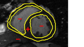
In cardiac image analysis, there are multiple structures (the right and left ventricles, and myocardium) that all useful and should be segmented. Our method is easily adaptable to this case. Indeed, computation of $v_{\tau}$ in Section III-C can be readily generalized. In general, multiple level sets should be used to represent multiple regions. However, in our case of interest (ventricles and surrounding epicardium), the regions form a rather simple topology (see Figure 3), and all regions can be represented using a single level set.

While theoretically $\phi_{\tau}$ for each $\tau$ will be an invertible/onto map in each individual region, and thus regions cannot change topology, numerically, between close by structures, merging/splitting may occur. Since we know that, in our application of interest, there is no such topology change, we enforce a hard topology constraint, that topology must not change during the level set evolution. This is now standard with level sets using discrete topology preserving techniques [14]. The original level set evolution is augmented with a step that looks for non-simple points that change sign in a level set update, i.e., locations of topology change. Such points are not allowed to change sign, and this preserves topology. Non-simple points are easily detected with local pixel-wise operations, and this makes implementation easy and the technique adds very little computational cost. The reader is referred to [14] for details on the criteria for simple points.

Figure 3: Representation of the right and left ventricles and myocardium with a single level set function (sign of level set function indicated in red in the regions bounded by yellow contours).

V Experiments

This section consists of four sets of experiments. The first two experiments are examples that illustrate and verify that our technique works as expected. The third and fourth experiments are the core experiments that show the main motivation of our algorithm: as a technique to improve the prediction step in interactive segmentation algorithms, which are predominantly used in commercial applications for cardiac analysis. These last experiments thus compares our technique to the popular and recent cardiac image segmentation software Medviso [15, 44].

V-A Synthetic Experiment

We start by verifying our registration and tracking technique on a synthetic sequence designed to mimic the piecewise deformation with matching normals for which our technique is designed. We consider a sequence composed of images with two textures (one for the object, and the other for the background). Textures are needed so that optical flow can be determined. The region of interest is the disc, and it along with the background contracts. In addition to the contraction, there is small rotational motions of the disc and the background in opposite directions. The sequence is constructed so that the normal component across the boundary matches in both regions. Note that this causes the true flow to be non-smooth across the boundary. Ground truth registration between consecutive images are known, and the deformation is not infinitesimal.

The first row of Figure 4 shows the first two frames of the synthetic sequence, the optical flow color code (whose color indicates direction and intensity of color indicates magnitude) and the ground truth optical flow for the first two frames. The second row shows registrations computed by global regularization with smoothness $\alpha_{i}=\alpha_{o}=\{3,20,50\}$ and the proposed method with $\alpha_{i}=\alpha_{o}=3$. Notice that global regularization smooths across the boundary, thus mixing inhomogeneous motions, leading to an inaccurate registration. Our proposed registration, which does not smooth across the boundary while satisfying the physical constraint, is able to accurately recover the true registration.

Figure 5 displays the results of tracking the whole synthetic sequence of 10 frames (only 4 are shown) with registration that uses global regularization and our method. The first three rows display the result of tracking using global regularization with smoothness $\alpha_{i}=\alpha_{o}=\{3,20,50\}$. Notice that global regularization of the deformation with small global regularization ($\alpha_{i}=\alpha_{o}=3$) leads to less smoothing across the boundary, but an inaccurate segmentation due to small regularization which traps the contour in small scale structures. Larger global regularization smooths more across the boundary leading to an inaccurate registration. The segmentation improves, but the boundary is still not captured accurately. No amount of global regularization is able to detect an accurate boundary. Finally, our method (last row), which smooths within regions while simultaneously satisfying the normal matching constraint is able to capture both an accurate registration and segmentation.

image	next image	color code	ground truth
global, $\alpha=3$	global, $\alpha=20$	global, $\alpha=50$	our method

Figure 4: Global vs. Physically Motivated Registration on Synthetic Images. [Top]: First two frames of the sequence, optical flow color map, and ground truth registration between images (two regions of differing motion and matching normals on the boundary). [Bottom]: Optical flow computed using global regularization $\alpha=\{3,20,50\}$, and by the proposed method with smoothness $\alpha_{i}=\alpha_{o}=3$. The proposed method recovers the true registration while no amount of global regularization recovers the true registration.

initial	tracked (red-algorithm, yellow-ground truth)
global $\alpha\!=\!3$
global $\alpha\!=\!20$
global $\alpha\!=\!50$
our method

Figure 5: Global vs. Physically Motivated Tracking on Synthetic Sequence. [First three rows]: Region tracking using global regularization with $\alpha=\{3,20,50\}$. [Last row]: proposed method. Since the proposed technique is able to better capture the underlying registration than global regularization, it also has higher accuracy in segmentation of the circular object.

V-B Ventricle Segmentation: Comparison of Three Registration Schemes

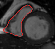
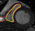
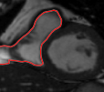
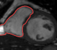
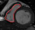
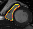
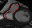
In this experiment, we focus on real cardiac MRI data and compare registration methods used for segmentation of the LV and RV. We visually compare the tracking results given by our method to (M1) registration of only the interior of current estimate of the ventricle to a subset of next image (to show whole image registration is needed), and to (M2) standard full image registration with global smoothness. M1 is achieved by computing just the inside velocity with Neumann boundary conditions on $\partial R_{\tau}$ (normal constraint does not apply in M1). The best results with respect to ground truth are chosen by choosing the optimal parameter $\alpha$ in all methods. Results on LV and RV tracking for a full cardiac cycle are given in Figure 6 for the LV and Figure 7 for the RV. Registering only the organ (M1) results in errors (as the background registration is helpful in restricting undesirable registrations of the foreground). Globally smooth registration (M2) smooths motion from irrelevant background structures into the ventricles, which results in drifting from the desired boundary. Our method, which smooths within regions with satisfying the physical constraint, is able to achieve the most accurate results.

initial	ventricle tracked (red - algorithm result, yellow - ground truth)
region registration
global smoothing
our method

Figure 6: Illustrative Differences of Registration Schemes on the LV. [Top]: registering only the inside of the ventricle leads to inaccurate segmentation in subsequent frames. [Middle]: registering the whole image with global regularization smooths motion across different structures and leads to inaccurate segmentation. [Bottom]: registering the entire image with proposed technique leads to the most accurate segmentation. Green: initialization, red: algorithm result, yellow: ground truth.

initial	ventricle tracked (red - algorithm result, yellow - ground truth)
region registration
global smoothing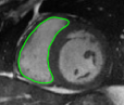
our method

Figure 7: Illustrative Differences of Registration Schemes on the RV. [Top]: registering only the inside of the ventricle leads to inaccurate segmentation in subsequent frames. [Middle]: registering the whole image with global regularization smooths motion across different structures and leads to inaccurate segmentation. [Bottom]: registering the entire image with proposed technique leads to the most accurate segmentation. Green: initialization, red: algorithm result, yellow: ground truth.

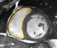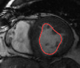
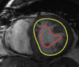
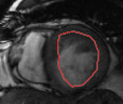
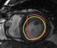
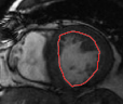
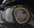
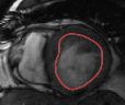
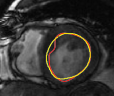
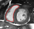
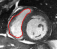
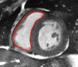
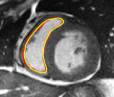
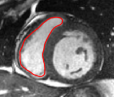
V-C LV and RV Segmentation: Quantitative Comparison to Commercial Software

We show experiments demonstrating the main use of our algorithm: in improving the prediction step of interactive segmentation methods. We show that less interaction is needed with our approach than a recent and widely used commercial cardiac segmentation software, Segment from Medviso [15, 44]. We perform quantitative assessment of the tracking performance of our method and compare it to Medviso. The evaluation was carried out on publicly available data sets, the MICCAI Left Ventricle Dataset [37] and the MICCAI Right Ventricle Dataset [25]. The validation dataset from [37] consists of 15 sets of cardiac cine-MRI images. Each set contains 6 to 20 2D slices from a 3D image, with each slice having 20 images of the cardiac phases. Similarly, the data set [25] contains 16 sets of cardiac cine-MRI images, each containing about 10 slices of 20 phases each. These data sets contain ground truth segmentations for left and right ventricles respectively (unfortunately ground truth for both the LV and RV is not available on a single dataset that we are aware of). Both methods start with the same initially correct segmentation, and subsequent frames are segmented via propagation. No manual interaction is used as we wish to show that our method would require less interaction. The regularity parameter $\alpha=\alpha_{i}=\alpha_{o}$ in our method is found by choosing $\alpha$ so that the results are closest to ground truth in a few training cases. The same parameter is then used for all other cases.

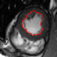
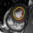
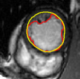
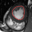
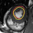
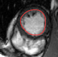
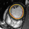
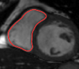
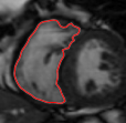
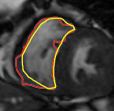
Figures 8 and 9 shows some sample tracking results of the proposed method and Medviso on full cardiac cycles of two different cases on both the LV dataset and the RV dataset. The ground truth (yellow) is superimposed when available. A summary of the results on the entire datasets is shown in Table I. The accuracy with respect to ground truth is measured using average perpendicular distance (APD) and dice metric (DM) for left ventricle, and Hausdorff distance (HD) and DM for the right ventricle. These metrics are chosen since they are the standard ones used on these datasets. Both qualitative and quantitative results show that our proposed method leads to more accurate segmentation of the ventricles and thus leads to less interaction than segmentation propagation schemes in than Medviso.

initial	ventricle tracked (red - algorithm result, yellow - ground truth)
Medviso
our method
Medviso
our method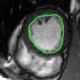

Figure 8: Comparison on Tracking the Left Ventricle. Two sample results on the MICCAI LV Dataset of full cardiac cycles (only 5 out of 20 images are shown) of the proposed algorithm and Medviso. The ground truth when available is shown in yellow is superimposed when available, and the red contour is the result obtained by the indicated algorithm. Visual results indicate that our algorithm is better able to handle non-homogenous appearance, and is thus more accurate.

initial	ventricle tracked (red - algorithm result, yellow - ground truth)
Medviso
our method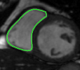
Medviso
our method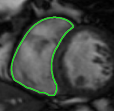

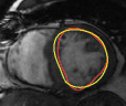
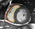
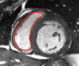
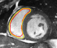
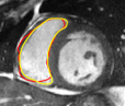
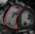
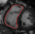
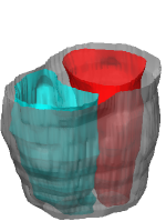
Figure 9: Comparison on Tracking the Right Ventricle Two sample results on the MICCAI RV Dataset of full cardiac cycles (only 5 out of 20 images are shown) of the proposed algorithm and Medviso. The ground truth when available is shown in yellow is superimposed when available, and the red contour is the result obtained by the indicated algorithm. Visual results indicate that our method is less susceptible to clutter nearby the RV, and thus is able to capture the RV more accurately.

	MICCAI LV		MICCAI RV
mean $\pm$ std	APD	DM	HD	DM
Ours	2.39$\pm$ .31	.88$\pm$.02	6.72 $\pm$ 3.22	.83$\pm$.15
MedViso	4.68$\pm$ 1.2	.78$\pm$.09	15.19 $\pm$ 6.08	.73$\pm$.19

TABLE I: Quantitative Evaluation on the MICCAI LV validation [37] and MICCAI RV training [25] datasets. Low APD/HD and high DM indicate good matches.

V-D Multiple Region Segmentation: Full Heart Segmentation

We now demonstrate our approach in performing challenging full heart segmentation: segmentation of the ventricles and epicardium all in one shot. Both the RV and epicardium are especially challenging as the contrast of the RV and background is subtle in comparison to the LV, and the myocardium wall near parts of the RV is very thin. We are not aware of another interactive method that is able to segment all structures, and so we compare to Medviso even though the method is not specifically tailored to the myocardium, but the method is generic and is able to propagate a segmentation. Further, Medviso does not segment multiple regions all at once and thus we perform separate segmentation of the LV, RV and epicardium. Since ground truth is not available for the outer wall of the myocardium in any standard dataset that we aware of, we show visual comparison.

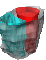
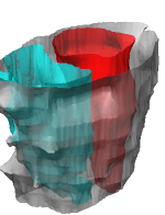
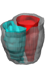
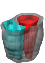
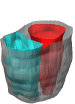
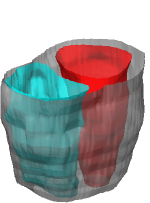
Figure 10 shows the slice-wise results of our method and Medviso on a full 3D cardiac MRI sequence for a full cardiac cycle. Results indicate that our method is more accurate in capturing the shape of the ventricles and epicardium, and our method is especially more promising on the RV and epicardium. Figure 11 shows visualization of the results in 3D, and that our method more accurately resembles the structure of the heart.

Figure 10: Comparison on Multiple Region Segmentation. [Top to Bottom]: $1^{st},3^{rd},6^{th}$ and $8^{th}$ slices shown. The LV (red), RV (cyan) and myocardium outer boundary (yellow) are simultaneously segmented using our proposed technique. Comparison is shown to Medviso. Visual results indicate that our technique is more accurate in segmenting all structures.

tracked in time $\rightarrow$
Medviso   
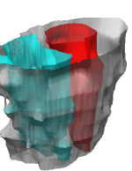
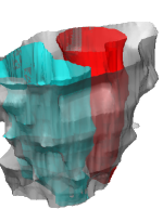
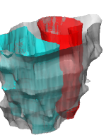
our method   

Figure 11: Comparison on Multiple Region Segmentation (3D Visualization). [Top row]: Medviso result, [Bottom row]: our result. Grey: Myocardium, cyan: right ventricle, red: left ventricle. Only 5 of 20 frames shown. Results indicate that the results of our method resemble heart structure.

VI Conclusion

We have presented an algorithm for propagating the segmentation from one frame in an image sequence to another via a novel registration algorithm. The registration is physically motivated by the multi-modal motions among sub-structures and the physical constraints between motions in adjacent regions, specifically the matching conditions of normal velocities. Traditional registration algorithms apply global regularization smoothing across region boundaries, mixing motions of differing sub-structures, are not physically motivated, and therefore yield inaccurate registrations and therefore segmentation propagations. The presented technique solves the registration via a variational formulation that results in PDEs in regions coupled via boundary conditions that resemble Robin boundary conditions. This leads to a computationally efficient technique that has the same cost as traditional regularization.

Experiments have shown that our method is more effective than global regularization in propagating segmentations in cardiac MRI data of the heart. Moreover, the main motivation for this work has been to improve existing interactive segmentation techniques, which are commonly used commercially, for cardiac MRI segmentation by better predicting a segmentation in the next frame from the current frame. We have compared our technique both qualitatively and quantitatively against a recent and widely used commercial software, Medviso, and results indicate that our method would require less manual interaction for segmentation correction, specifically in LV, RV and epicardium segmentation.

Appendix A Proof of Positive-Definiteness of Motion Operators

This appendix shows that the PDEs with the boundary conditions (21) and (22) (and similarly (12) and (13) in the previous subsection) can be solved with a conjugate gradient solver by showing the corresponding linear operators are positive-semi definite. This can be shown by considering the following standard $\mathbb{L}^{2}$ inner product on the space of admissible velocities $v_{i},v_{o}$:

$$\left<{v^{1}},{v^{2}}\right>=\int_{R}v^{1}_{i}\cdot v^{2}_{i}\,\mathrm{d}x+\int_{\Omega\backslash R}v^{1}_{o}\cdot v^{2}_{o}\,\mathrm{d}x.$$

Given the operator $A=(-\alpha_{i}\Delta+\nabla I\nabla I^{T},\,-\alpha_{o}\Delta+\nabla I\nabla I)$ acting on $v=(v_{i},v_{o})$, positive semi-definiteness is shown by verifying $\left<{Av},{v}\right>\geq 0$:

$$\left<{Av},{v}\right> =\int_{R}(-\alpha_{i}\Delta v_{i}+\nabla I\nabla I^{T}v_{i})\cdot v_{i}\,\mathrm{d}x+\int_{R}(-\alpha_{o}\Delta v_{o}+\nabla I\nabla I^{T}v_{o})\cdot v_{o}\,\mathrm{d}x$$

$$=\int_{R}\alpha_{i}|\nabla v_{i}|^{2}+(\nabla I\cdot v_{i})^{2}\,\mathrm{d}x+\int_{\Omega\backslash R}\alpha_{o}|\nabla v_{o}|^{2}+(\nabla I\cdot v_{o})^{2}\,\mathrm{d}x$$

$$-\int_{\partial R}\alpha_{i}(\nabla v_{i}\cdot N)\cdot v_{i}-\alpha_{o}(\nabla v_{o}\cdot N)\cdot v_{o}\,\mathrm{d}s$$

$$=\int_{R}\alpha_{i}|\nabla v_{i}|^{2}+(\nabla I\cdot v_{i})^{2}\,\mathrm{d}x+\int_{\Omega\backslash R}\alpha_{o}|\nabla v_{o}|^{2}+(\nabla I\cdot v_{o})^{2}\,\mathrm{d}x\geq 0.$$

The last equality is due to the vanishing boundary integrals, which is obtained by noting the boundary conditions (14) and (15) or (23)-(26). Indeed, noting (14) and (15), we have that $\alpha_{i}(\nabla v_{i}\cdot N)=\alpha_{o}(\nabla v_{o}\cdot N)$, which implies the vanishing boundary term above. Similarly, (23)-(26) implies that

$$\alpha_{i}(\nabla v_{i}\cdot N)\cdot v_{i}-\alpha_{o}(\nabla v_{o}\cdot N)\cdot v_{o}=\alpha_{i}(\nabla v_{i}\cdot N)\cdot N(v_{i}\cdot N)-\alpha_{o}(\nabla v_{o}\cdot N)\cdot N(v_{o}\cdot N)=0.$$

Thus, since positive definiteness is shown, the conjugate gradient algorithm may be applied.

References

- [1] M. Beg, M. Miller, A. Trouvé, and L. Younes. Computing large deformation metric mappings via geodesic flows of diffeomorphisms. International Journal of Computer Vision, 61(2):139–157, 2005.
- [2] Y. Boykov and M. Jolly. Interactive organ segmentation using graph cuts. In Medical Image Computing and Computer-Assisted Intervention–MICCAI 2000, pages 147–175. Springer, 2000.
- [3] Y. Boykov, O. Veksler, and R. Zabih. Fast approximate energy minimization via graph cuts. Pattern Analysis and Machine Intelligence, IEEE Transactions on, 23(11):1222–1239, 2001.
- [4] X. Bresson, S. Esedoḡlu, P. Vandergheynst, J.-P. Thiran, and S. Osher. Fast global minimization of the active contour/snake model. Journal of Mathematical Imaging and vision, 28(2):151–167, 2007.
- [5] Y. Chen, H. D. Tagare, S. Thiruvenkadam, F. Huang, D. Wilson, K. S. Gopinath, R. W. Briggs, and E. A. Geiser. Using prior shapes in geometric active contours in a variational framework. International Journal of Computer Vision, 50(3):315–328, 2002.
- [6] T. Cootes, G. Edwards, and C. Taylor. Active appearance models. IEEE Transactions on Pattern Analysis and Machine Intelligence, 23(6):681–685, 2001.
- [7] T. Cootes, C. Taylor, D. Cooper, J. Graham, et al. Active shape models-their training and application. Computer vision and image understanding, 61(1):38–59, 1995.
- [8] L. Cordero-Grande, G. Vegas-Sánchez-Ferrero, P. Casaseca-de-la Higuera, J. Alberto San-Román-Calvar, A. Revilla-Orodea, M. Martín-Fernández, and C. Alberola-López. Unsupervised 4d myocardium segmentation with a markov random field based deformable model. Medical Image Analysis, 15(3):283–301, 2011.
- [9] D. Cremers, O. Fluck, M. Rousson, and S. Aharon. A probabilistic level set formulation for interactive organ segmentation. In Medical Imaging, pages 65120V–65120V. International Society for Optics and Photonics, 2007.
- [10] D. Cremers, T. Kohlberger, and C. Schnörr. Shape statistics in kernel space for variational image segmentation. Pattern Recognition, 36(9):1929–1943, 2003.
- [11] D. Cremers and S. Soatto. Motion competition: A variational approach to piecewise parametric motion segmentation. International Journal of Computer Vision, 62(3):249–265, 2005.
- [12] D. G. Ebin and J. Marsden. Groups of diffeomorphisms and the motion of an incompressible fluid. The Annals of Mathematics, 92(1):102–163, 1970.
- [13] O. Ecabert, J. Peters, H. Schramm, C. Lorenz, J. von Berg, M. J. Walker, M. Vembar, M. E. Olszewski, K. Subramanyan, G. Lavi, et al. Automatic model-based segmentation of the heart in ct images. Medical Imaging, IEEE Transactions on, 27(9):1189–1201, 2008.
- [14] X. Han, C. Xu, and J. L. Prince. A topology preserving level set method for geometric deformable models. Pattern Analysis and Machine Intelligence, IEEE Transactions on, 25(6):755–768, 2003.
- [15] E. Heiberg, J. Sjögren, M. Ugander, M. Carlsson, H. Engblom, and H. Arheden. Design and validation of segment-freely available software for cardiovascular image analysis. BMC medical imaging, 10(1):1, 2010.
- [16] T. Heimann and H.-P. Meinzer. Statistical shape models for 3d medical image segmentation: A review. Medical image analysis, 13(4):543–563, 2009.
- [17] B. K. Horn and B. G. Schunck. Determining optical flow. Artificial intelligence, 17(1):185–203, 1981.
- [18] I. Isgum, M. Staring, A. Rutten, M. Prokop, M. Viergever, and B. van Ginneken. Multi-atlas-based segmentation with local decision fusion—application to cardiac and aortic segmentation in ct scans. IEEE Transactions on Medical Imaging, pages 1000–1010, 2009.
- [19] M. Kass, A. Witkin, and D. Terzopoulos. Snakes: Active contour models. International journal of computer vision, 1(4):321–331, 1988.
- [20] M. Kaus, J. Berg, J. Weese, W. Niessen, and V. Pekar. Automated segmentation of the left ventricle in cardiac mri. Medical Image Analysis, 8(3):245–254, 2004.
- [21] H. A. Kirisli, M. Schaap, S. Klein, L. A. Neefjes, A. C. Weustink, T. Walsum, and W. J. Niessen. Fully automatic cardiac segmentation from 3d cta data: a multi-atlas based approach. In Proc. of SPIE Vol, volume 7623, pages 762305–1, 2010.
- [22] J. Koikkalainen, T. Tolli, K. Lauerma, K. Antila, E. Mattila, M. Lilja, and J. Lotjonen. Methods of artificial enlargement of the training set for statistical shape models. Medical Imaging, IEEE Transactions on, 27(11):1643–1654, 2008.
- [23] A. Lalande, L. Legrand, P. M. Walker, F. Guy, Y. Cottin, S. Roy, and F. Brunotte. Automatic detection of left ventricular contours from cardiac cine magnetic resonance imaging using fuzzy logic. Investigative radiology, 34(3):211–217, 1999.
- [24] X. Lin, B. R. Cowan, and A. A. Young. Automated detection of left ventricle in 4d mr images: experience from a large study. In Medical Image Computing and Computer-Assisted Intervention–MICCAI 2006, pages 728–735. Springer, 2006.
- [25] Litis. Rv segmentation challenge in cardiac mri, 2012.
- [26] M. Lorenzo-Valdes, G. Sanchez-Ortiz, R. Mohiaddin, and D. Rueckert. Segmentation of 4d cardiac mr images using a probabilistic atlas and the em algorithm. In Medical Image Computing and Computer-Assisted Intervention-MICCAI 2003: 6th International Conference, Montreal, Canada, November 15-18, 2003, Proceedings, volume 1, page 440. Springer, 2004.
- [27] J. Lötjönen, S. Kivistö, J. Koikkalainen, D. Smutek, and K. Lauerma. Statistical shape model of atria, ventricles and epicardium from short-and long-axis mr images. Medical image analysis, 8(3):371–386, 2004.
- [28] M. Lynch, O. Ghita, and P. F. Whelan. Automatic segmentation of the left ventricle cavity and myocardium in mri data. Computers in Biology and Medicine, 36(4):389–407, 2006.
- [29] B. R. Munson, D. F. Young, and T. H. Okiishi. Fundamentals of fluid mechanics. New York, 1990.
- [30] N. M. Noble, D. L. Hill, M. Breeuwer, J. A. Schnabel, D. J. Hawkes, F. A. Gerritsen, and R. Razavi. Myocardial delineation via registration in a polar coordinate system. In Medical Image Computing and Computer-Assisted Intervention—MICCAI 2002, pages 651–658. Springer, 2002.
- [31] S. Osher and J. Sethian. Fronts propagating with curvature-dependent speed: algorithms based on hamilton-jacobi formulations. Journal of computational physics, 79(1):12–49, 1988.
- [32] D. F. Pace, A. Enquobahrie, H. Yang, S. R. Aylward, and M. Niethammer. Deformable image registration of sliding organs using anisotropic diffusive regularization. In Biomedical Imaging: From Nano to Macro, International Symposium on, pages 407–413. IEEE, 2011.
- [33] N. Paragios. A variational approach for the segmentation of the left ventricle in cardiac image analysis. International Journal of Computer Vision, 50(3):345–362, 2002.
- [34] N. Paragios. A level set approach for shape-driven segmentation and tracking of the left ventricle. IEEE Transactions on Medical Imaging, 22(6):773–776, 2003.
- [35] C. Petitjean and J. Dacher. A review of segmentation methods in short axis cardiac mr images. Medical image analysis, 15(2), 2011.
- [36] Q. Pham, F. Vincent, P. Clarysse, P. Croisille, and I. Magnin. A fem-based deformable model for the 3d segmentation and tracking of the heart in cardiac mri. In Image and Signal Processing and Analysis, 2001. ISPA 2001. Proceedings of the 2nd International Symposium on, pages 250–254. IEEE, 2001.
- [37] P. Radau, Y. Lu, K. Connelly, G. Paul, A. Dick, and G. Wright. Evaluation framework for algorithms segmenting short axis cardiac mri. Midas Journal, 2009.
- [38] L. Risser, H. Baluwala, and J. A. Schnabel. Diffeomorphic registration with sliding conditions: Application to the registration of lungs ct images. In Fourth International Workshop on Pulmonary Image Analysis, MICCAI, pages 79–90, 2011.
- [39] J. Schaerer, C. Casta, J. Pousin, and P. Clarysse. A dynamic elastic model for segmentation and tracking of the heart in mr image sequences. Medical Image Analysis, 14(6):738–749, 2010.
- [40] A. Schmidt-Richberg, J. Ehrhardt, R. Werner, and H. Handels. Fast explicit diffusion for registration with direction-dependent regularization. Biomedical Image Registration, pages 220–228, 2012.
- [41] J. A. Schnabel, D. Rueckert, M. Quist, J. M. Blackall, A. D. Castellano-Smith, T. Hartkens, G. P. Penney, W. A. Hall, H. Liu, C. L. Truwit, et al. A generic framework for non-rigid registration based on non-uniform multi-level free-form deformations. In Medical Image Computing and Computer-Assisted Intervention–MICCAI 2001, pages 573–581. Springer, 2001.
- [42] J. Senegas, C. A. Cocosco, and T. Netsch. Model-based segmentation of cardiac mri cine sequences: a bayesian formulation. In Medical Imaging 2004, pages 432–443. International Society for Optics and Photonics, 2004.
- [43] M. Sermesant, P. Moireau, O. Camara, J. Sainte-Marie, R. Andriantsimiavona, R. Cimrman, D. L. Hill, D. Chapelle, and R. Razavi. Cardiac function estimation from mri using a heart model and data assimilation: advances and difficulties. Medical Image Analysis, 10(4):642–656, 2006.
- [44] J. Sjögren, J. F. Ubachs, H. Engblom, M. Carlsson, H. Arheden, E. Heiberg, et al. Semi-automatic segmentation of myocardium at risk in t2-weighted cardiovascular magnetic resonance. J Cardiovasc Magn Reson, 14(10), 2012.
- [45] M. Stegmann, H. Ólafsdóttir, and H. Larsson. Unsupervised motion-compensation of multi-slice cardiac perfusion mri. Medical Image Analysis, 9(4):394–410, 2005.
- [46] A. Tsai, A. Yezzi Jr, W. Wells, C. Tempany, and et al. A shape-based approach to the segmentation of medical imagery using level sets. IEEE Transactions on Medical Imaging, 22(2):137–154, 2003.
- [47] H. Van Assen, M. Danilouchkine, A. Frangi, S. Ord s, J. Westenberg, J. Reiber, and B. Lelieveldt. Spasm: A 3d-asm for segmentation of sparse and arbitrarily oriented cardiac mri data. Medical Image Analysis, 10(2):286–303, 2006.
- [48] T. Vercauteren, X. Pennec, A. Perchant, and N. Ayache. Symmetric log-domain diffeomorphic registration: A demons-based approach. MICCAI, pages 754–761, 2008.
- [49] X. Xue. Interactive 3d heart chamber partitioning with a new marker-controlled watershed algorithm. In G. Bebis, R. Boyle, D. Koracin, and B. Parvin, editors, Advances in Visual Computing, volume 3804 of Lecture Notes in Computer Science, pages 92–99. Springer Berlin Heidelberg, 2005.
- [50] H. Zhang, A. Wahle, R. Johnson, T. Scholz, and M. Sonka. 4-d cardiac mr image analysis: left and right ventricular morphology and function. Medical Imaging, IEEE Transactions on, 29(2):350–364, 2010.
- [51] S. Zhang, Y. Zhan, M. Dewan, J. Huang, D. Metaxas, and X. Zhou. Deformable segmentation via sparse shape representation. MICCAI, pages 451–458, 2011.
- [52] Y. Zhu, X. Papademetris, A. J. Sinusas, and J. S. Duncan. Segmentation of the left ventricle from cardiac mr images using a subject-specific dynamical model. Medical Imaging, IEEE Transactions on, 29(3):669–687, 2010.
- [53] X. Zhuang. Challenges and methodologies of fully automatic whole heart segmentation: A review.
- [54] X. Zhuang, K. Rhode, R. Razavi, D. Hawkes, and S. Ourselin. A registration-based propagation framework for automatic whole heart segmentation of cardiac mri. Medical Imaging, IEEE Transactions on, 29(9):1612–1625, 2010.