First simultaneous measurement of sextupolar and octupolar resonance driving terms in a circular accelerator from turn-by-turn beam position monitors data

A. Franchi*** L. Farvacque, F. Ewald, G. Le Bec, K. B. Scheidt andrea.franchi@esrf.fr ESRF, Grenoble, France
Abstract

Beam lifetime in storage rings and colliders is affected by , among other effects, lattice nonlinearities. Their control are of great benefit to the dynamic aperture of an accelerator, whose enlargement leads in general to more efficient injection and longer lifetime. This article describes a procedure to evaluate and correct unwanted nonlinearities by using turn-by-turn beam position monitor data, which is an evolution of previous works on the resonance driving terms (RDTs). Effective sextupole magnetic errors and tilts at the ESRF electron storage ring are evaluated and corrected (when possible) by using this technique. For the first time, also octupolar RDTs could be measured and used to define an octupolar model for the main quadrupoles. Most of the deviations from the model observed in the sextupolar RDTs of the ESRF storage ring turned out to be generated by focusing errors rather than by sextupole errors. These results could be achieved thanks to new analytical formulas describing the harmonic content of the nonlinear betatron motion to the second order. For the first time, RDTs have been also used for beam-based calibration of individual sextupole magnets. They also proved to be a powerful tool in predicting faulty magnets and in validating magnetic models. This technique provides also a figure of merit for a self-assessment of the reliability of the data analysis.

I Introduction and motivation

Many factors make the implementation of a magnetic optics in a circular accelerator different from the nominal one: deviations from the magnet calibration curves and from the ideal magnetic lengths, displacements from the reference position and axis, unknown multipole components, and the like. This generally results in machine performances below expectations: low beam lifetime and dynamic aperture, poor injection efficiency, large emittances (in lepton machines) and limited luminosity (in colliders).

While an artillery of different methods and algorithms has been developed and successfully implemented in routine operation for the evaluation and correction of focusing errors (linear optics) and betatron coupling, their extension to the nonlinear modelling and correction remains difficult, because either time-consuming or requiring diagnostic tools unavailable a decade ago. In most cases, such as at the ESRF storage ring, the correction of the nonlinear optics is done by trials and errors seeking heuristically longer lifetime. Nevertheless, the installation of beam position monitors (BPMs) with turn-by-turn (TbT) acquisition system in many circular accelerators and the parallel development of a theoretical formalism for the description of the harmonic content of the acquired data paved the way for more rapid and deterministic measurement and correction of the nonlinear optics. This paper proposes a new method aiming at such characteristics.

Several approaches for the evaluation of the nonlinear lattice model exist and any attempt to offer a coverage of the pertinent literature would be incomplete. However, in the context of this paper a few works may be recalled, either for their proximity or because they represented milestones for this work. A pioneering work on the exploitation of TbT BPM data dates back to the early ’90s Caussyn . The application of the normal form approach Turchetti1 ; Forest1 to single-particle tracking data of Ref. Bartolini1 introduced for the first time an explicit correspondence between spectral lines of TbT data and resonance driving terms (RDTs). A breakthrough was represented by the experience at the CERN Super Proton Synchrotron, where sextupolar RDTs along the entire ring were measured and used to detect faulty sextupole magnets Rogelio1 and to extract strength and polarity of some sextupoles Andrea-thesis ; prstab_strength . More recently independent component analysis (ICA) was applied to TbT BPM data for the extraction of lattice linear and nonlinear properties LosAlamos . Of interest are also the experimental results of Ref. Bartolini2 , where the nonlinear model was fit to the spectral content of TbT data, even though not via the RDTs. In Ref. RDT-PS simultaneous measurements of two RDTs, one sextupolar and one octupolar, are reported.

The paper is structured as follows. After highlighting and anticipating both advantages and limitations of the proposed method in Sec. II, the technique is introduced and discussed in its main results in Sec. III (all mathematical derivations are put in separate appendices). The experimental results of the new method in evaluating the nonlinear model, calibrating sextupole magnets and computing a corrector setting are presented in Sec. IV. The evaluation of octupolar terms in the lattice from the same TbT data is described in Sec. V.

II Novelties and limitations of the proposed method

The main novelties of the proposed scheme (compared to other methods for the measurement and correction of nonlinear lattice model) may be listed as follows: (i)𝑖(i) The harmonic analysis is performed on the pure position data x𝑥x (y𝑦y), rather than on the complex signal xipx𝑥𝑖subscript𝑝𝑥x-ip_{x} (yipy𝑦𝑖subscript𝑝𝑦y-ip_{y}) of Ref. Bartolini1 ; Rogelio1 , hence with no concern about errors in the evaluation of the momentum pxsubscript𝑝𝑥p_{x} (pysubscript𝑝𝑦p_{y}) and about BPM synchronization; (ii)𝑖𝑖(ii) The possibility of measuring at the same time linear combinations of all sextupolar (normal and skew) and most of octupolar RDTs offers a complete and simultaneous picture of all resonances at a given working point, rather than having to shift the tunes close to a single resonant condition to excite a specific mode, as in Ref. LosAlamos ; (iii)𝑖𝑖𝑖(iii) The nonlinear problem of inferring sextupole and octupole strengths from the betatron beam motion is translated into a linear system to be inverted (with due preliminary precautions) when RDTs are used as observables, hence rendering the model fit and correction straightforward; (iv)𝑖𝑣(iv) Last but not least, the quality of the analysis of sextupolar RDTs may be self-assessed, so to optimize the experimental conditions as well as the initial lattice model.

Of course, this approach suffers from some practical limitations too.

First, the quality of the analysis is limited by the spectral resolution, here defined as the ratio between the amplitudes of the harmonics and the background noise. The resolution scales with the number of turns of acquired data exploitable for a Fast Fourier Transform (FFT). Ideally, the greater the number of turns with exploitable data, the higher the spectral resolution and hence the quality of the RDT measurement. Data filtering and interpolation Laskar ; TuneMeasBazzani , may provide excellent resolution already with tens of turns, though the presence of noise Zimmermann-book and the need of detecting spectral lines whose amplitudes are orders of magnitude lower than the tune line necessitate several hundred of exploitable oscillation turns. Chromaticity and decoherence (induced by nonzero amplitude dependent detuning) modulate and damp the TbT signal Chao . This multi-particle effect is not contemplated here, the baseline model being of a beam moving rigidly as a single particle. Most of the operational settings optimized for beam lifetime and stability result in nonzero chromaticity and detuning with amplitude. In the case of the ESRF storage ring, the exploitable number of turns ranges from about 30 to 60 turns, depending on the optics put in operation, insufficient to detect sextupolar harmonics whose amplitude is typically 2 or 3 orders of magnitude lower than the tune line. Therefore, a special optics was designed to provide almost zero linear chromaticity and detuning. For hadron machines this may be sufficient to obtain thousands of exploitable TbT data, as in Ref. LosAlamos . In lepton machines radiation damping depresses naturally the TbT signal. At the ESRF storage ring, the damping time being of about 2500 turns, the signal is sufficiently depressed to compromise the whole measurement already after 1024 turns (see Fig. 23). Usually either 256 or 512 turns are used for the FFT, as radiation damping would enhance the background spectral noise.

Second in the list of limitations is the BPM electronic resolution and noise. The commercial Libera Brilliance Libera BPMs installed in the ESRF storage ring are equipped with a standard electronic filter that covers several turns, resulting in TbT data corrupted from the neighbor turns. Even though a convolution may be carried out to extract clean TbT data, the spectral resolution remained insufficient for a detailed nonlinear analysis. A great improvement was achieved when implementing a moving-average filter (MAF) MAF . All results presented here are based on acquisitions carried out with this filter.

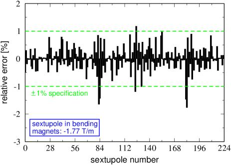
The dedicated optics designed and implemented for having zero chromaticity and amplitude detuning sets a limit on the capability of inferring sextupole errors for other operational optics, these having different sextupole settings. A way out would be to evaluate the relative field error for each magnet and to export it in all other optics, though this assumes that the relative errors are constant along the entire range of sextupole currents (i.e. strengths). The situation at the ESRF storage ring turned out to be rather relaxed in this sense, because almost all sextupole errors inferred from this method lay well within the specified ±1%plus-or-minuspercent1\pm 1\%. Moreover, most of the deviations observed from the ideal model are originated by the focusing errors, through the modulated beta functions present in the definitions of the RDTs. A first correction, hence, may be carried out by assuming ideal sextupoles and using the best linear model (easy to infer with other techniques) to evaluate the modulated RDTs and use sextupole correctors to restore at the best their periodicity.

A last limitation is linked to the linear system to be pseudo-inverted to extract the nonlinear model. The singular value decomposition (SVD) has been used for this purpose. The resulting model shall be then considered as effective and the inferred sextupole errors depend clearly on the numerical parameters (such as number of eigen-vectors, choice of weights among different possible sources of errors, and the like).

III Combined resonance driving terms from (dual-plane) BPM data

III.1 Theoretical introduction
Refer to caption

Refer to caption

Refer to caption

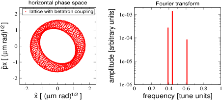
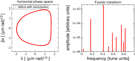
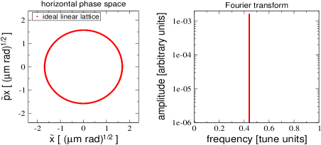
Figure 1: Three examples of phase space trajectory of a displaced particle in Courant-Snyder coordinates and corresponding Fourier coefficients (amplitudes): ideally linear (top), with betatron coupling (centre) and sextupoles (bottom). The fractional parts of the tunes in this example are Qx=0.44subscript𝑄𝑥0.44Q_{x}=0.44 and Qy=0.39subscript𝑄𝑦0.39Q_{y}=0.39.

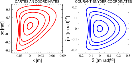
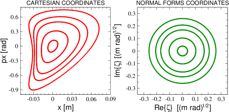
A charged particle circulating inside a circular accelerator or storage ring will execute a turn-by-turn oscillation around the closed orbit, if displaced transversely by a pulsed magnet, such as a magnet kicker. In phase space this oscillation describes a closed curve which reflects the local characteristics of the magnetic lattice. In an ideally linear machine this curve will be an ellipse. In the presence of strong sextupoles, at sufficiently large oscillation amplitudes the curve takes the shape of a triangle. With strong betatron coupling, the curves in the two transverse phase spaces (x,px)𝑥subscript𝑝𝑥(x,p_{x}) and (y,py)𝑦subscript𝑝𝑦(y,p_{y}) are linear combinations of the original ones. As long as the curve in phase space is closed and reasonably continuous (i.e. the motion is stable), the Fourier theorem ensures that it may be expressed as the sum of a series of sine or cosine terms (called the Fourier series), each of which has specific amplitude and phase coefficients known as Fourier coefficients. In other words, each closed curve may be described (after a linear transformation) as the superposition of circles. The harmonic content of the ideal ellipse in phase space will be represented by a single pair of amplitude and phase (the tune line): After the Courant-Snyder (C-S) transformation, the ellipse becomes a circle, whose radius corresponds to the amplitude and its position along the circumference is defined by the phase. Two additional harmonics (i.e. circles) are excited with betatron coupling (the tune of the other plane and its opposite). The triangular-shaped curve will instead require several harmonics to be properly described. The three examples are depicted in Fig. 1. Intuitively, the stronger the sextupoles, the more triangular is the horizontal phase space curve and the larger are the additional harmonics. It is indeed possible to correlate quantitatively (up to a certain precision) these deformations, and hence these harmonics, to the strengths of the magnets installed in the machine. More important, this correlation is in most cases linear with a precision much larger than the experimental resolution. The fundamental ingredient to establish this correlation is provided by the resonance driving terms (RDTs) of Refs. Bartolini1 ; Rogelio1 ; Andrea-thesis ; prstab_strength . These may be evaluated both from analytic formulas (rather simple in most cases) and from the harmonic analysis of the phase space curves, i.e. from their Fourier coefficients of the TbT BPM data. In Appendix A the theoretical description establishing this correlation is recalled and extended (when needed). The results of interest in the context of this paper are summarized in the next section.

Throughout the paper, all RDTs and machine parameters (linear and nonlinear) from the model are evaluated by MADX-PTC madx . Tracking simulations to simulate and validate the harmonic analysis of TbT BPM data have been also carried out with this code. No significant difference has been observed in the RDTs when representing sextupoles either as thin or thick elements and when including fringe fields. As far as nonlinear parameters (such as amplitude dependent detuning and chromaticity) are concerned, significant differences between the three representations appear and only the thick-lens model with fringe field has been used.

III.2 Theoretical results


Table 1: List of lines in the spectra of x~(N)~𝑥𝑁\tilde{x}(N) and y~(N)~𝑦𝑁\tilde{y}(N) with corresponding measurable combined RDTs (CRDTs) F=|F|eiqF𝐹𝐹superscript𝑒𝑖subscript𝑞𝐹F=|F|e^{iq_{F}} and excited resonances. A horizontal (vertical) spectral line H(nx,ny)𝐻subscript𝑛𝑥subscript𝑛𝑦H(n_{x},n_{y}) (V(nx,ny)𝑉subscript𝑛𝑥subscript𝑛𝑦V(n_{x},n_{y})) is located at the frequency nxQx+nyQysubscript𝑛𝑥subscript𝑄𝑥subscript𝑛𝑦subscript𝑄𝑦n_{x}Q_{x}+n_{y}Q_{y}. For each line, expressions for its amplitude and phase are given. The choice was made here to make use of the lines in the region [0,0.5] in tune units. First-order RDTs (defined in Table 3) are sufficient for coupling and normal sextupoles, while the analysis of skew sextupole terms requires a second-order analysis, through the observable RDTs (ORDTs) gjklmsubscript𝑔𝑗𝑘𝑙𝑚g_{jklm} of Table 14 (The justification for such a choice is given in Appendix C). Quadrupole errors are to be included in the model when computing the Courant-Snyder (C-S) parameters used to evaluate x~(N)~𝑥𝑁\tilde{x}(N), y~(N)~𝑦𝑁\tilde{y}(N) and the RDTs fjklm(1)superscriptsubscript𝑓𝑗𝑘𝑙𝑚1f_{jklm}^{(1)} of Table 3.
spectral line      amplitude phase ϕitalic-ϕ\phi Combined RDT    resonances magnetic term
H(1,0)𝐻10H(1,0) 12(2Ix)1/212superscript2subscript𝐼𝑥12\frac{1}{2}(2I_{x})^{1/2} ψx0subscript𝜓𝑥0\psi_{x0} normal quadrupole
V(0,1)𝑉01V(0,1) 12(2Iy)1/212superscript2subscript𝐼𝑦12\frac{1}{2}(2I_{y})^{1/2} ψy0subscript𝜓𝑦0\psi_{y0} normal quadrupole
H(0,1)𝐻01H(0,1) (2Iy)1/2|Fxy|superscript2subscript𝐼𝑦12subscript𝐹𝑥𝑦(2I_{y})^{1/2}|F_{xy}| qFxy+32π+ψy0subscript𝑞subscript𝐹𝑥𝑦32𝜋subscript𝜓𝑦0q_{F_{xy}}+\frac{3}{2}\pi+\psi_{y0} Fxy=f1001(1)f1010(1)subscript𝐹𝑥𝑦superscriptsubscript𝑓10011superscriptsubscript𝑓10101F_{xy}=f_{1001}^{(1)}-f_{1010}^{(1)*} (1,1),(1,-1) skew quadrupole
V(1,0)𝑉10V(1,0) (2Ix)1/2|Fyx|superscript2subscript𝐼𝑥12subscript𝐹𝑦𝑥(2I_{x})^{1/2}|F_{yx}| qFyx+32π+ψx0subscript𝑞subscript𝐹𝑦𝑥32𝜋subscript𝜓𝑥0q_{F_{yx}}+\frac{3}{2}\pi+\psi_{x0} Fyx=f1001(1)f1010(1)subscript𝐹𝑦𝑥superscriptsubscript𝑓10011superscriptsubscript𝑓10101F_{yx}=f_{1001}^{(1)*}-f_{1010}^{(1)*} (1,1),(1,-1) skew quadrupole
H(2,0)𝐻20H(-2,0) (2Ix)|FNS3|2subscript𝐼𝑥subscript𝐹𝑁𝑆3(2I_{x})|F_{NS3}| qFNS3+32π2ψx0subscript𝑞subscript𝐹𝑁𝑆332𝜋2subscript𝜓𝑥0q_{F_{NS3}}+\frac{3}{2}\pi-2\psi_{x0} FNS3=3f3000(1)f1200(1)subscript𝐹𝑁𝑆33superscriptsubscript𝑓30001superscriptsubscript𝑓12001F_{NS3}=3f_{3000}^{(1)}-f_{1200}^{(1)*} (1,0),(3,0) normal sextupole
H(0,2)𝐻02H(0,-2) (2Iy)|FNS2|2subscript𝐼𝑦subscript𝐹𝑁𝑆2(2I_{y})|F_{NS2}| qFNS2+32π2ψy0subscript𝑞subscript𝐹𝑁𝑆232𝜋2subscript𝜓𝑦0q_{F_{NS2}}+\frac{3}{2}\pi-2\psi_{y0} FNS2=f1020(1)f0120(1)subscript𝐹𝑁𝑆2superscriptsubscript𝑓10201superscriptsubscript𝑓01201F_{NS2}=f_{1020}^{(1)}-f_{0120}^{(1)} (1,-2),(1,2) normal sextupole
V(1,1)𝑉11V(-1,-1) (2Ix2Iy)1/2|FNS1|superscript2subscript𝐼𝑥2subscript𝐼𝑦12subscript𝐹𝑁𝑆1(2I_{x}2I_{y})^{1/2}|F_{NS1}| qFNS1+32πψx0ψy0subscript𝑞subscript𝐹𝑁𝑆132𝜋subscript𝜓𝑥0subscript𝜓𝑦0q_{F_{NS1}}+\frac{3}{2}\pi-\psi_{x0}-\psi_{y0} FNS1=2f1020(1)f0111(1)subscript𝐹𝑁𝑆12superscriptsubscript𝑓10201superscriptsubscript𝑓01111F_{NS1}=2f_{1020}^{(1)}-f_{0111}^{(1)*} (1,-2),(1,0) normal sextupole
V(1,1)𝑉11V(1,-1) (2Ix2Iy)1/2|FNS0|superscript2subscript𝐼𝑥2subscript𝐼𝑦12subscript𝐹𝑁𝑆0(2I_{x}2I_{y})^{1/2}|F_{NS0}| qFNS0+32π+ψx0ψy0subscript𝑞subscript𝐹𝑁𝑆032𝜋subscript𝜓𝑥0subscript𝜓𝑦0q_{F_{NS0}}+\frac{3}{2}\pi+\psi_{x0}-\psi_{y0} FNS0=2f0120(1)f0111(1)subscript𝐹𝑁𝑆02superscriptsubscript𝑓01201superscriptsubscript𝑓01111F_{NS0}=2f_{0120}^{(1)}-f_{0111}^{(1)} (1,-2),(1,0) normal sextupole
V(0,2)𝑉02V(0,-2) (2Iy)|FSS3|2subscript𝐼𝑦subscript𝐹𝑆𝑆3(2I_{y})|F_{SS3}| qFSS3+32π2ψy0subscript𝑞subscript𝐹𝑆𝑆332𝜋2subscript𝜓𝑦0q_{F_{SS3}}+\frac{3}{2}\pi-2\psi_{y0} FSS3=3g0030g0012subscript𝐹𝑆𝑆33subscript𝑔0030superscriptsubscript𝑔0012F_{SS3}=3g_{0030}-g_{0012}^{*} (0,1),(0,3) skew sextupole
V(2,0)𝑉20V(-2,0) (2Ix)|FSS2|2subscript𝐼𝑥subscript𝐹𝑆𝑆2(2I_{x})|F_{SS2}| qFSS2+32π2ψx0subscript𝑞subscript𝐹𝑆𝑆232𝜋2subscript𝜓𝑥0q_{F_{SS2}}+\frac{3}{2}\pi-2\psi_{x0} FSS2=g2010,Vg0210subscript𝐹𝑆𝑆2subscript𝑔2010𝑉superscriptsubscript𝑔0210F_{SS2}=g_{2010,V}-g_{0210}^{*} (2,-1),(2,1) skew sextupole
H(1,1)𝐻11H(-1,-1) (2Ix2Iy)1/2|FSS1|superscript2subscript𝐼𝑥2subscript𝐼𝑦12subscript𝐹𝑆𝑆1(2I_{x}2I_{y})^{1/2}|F_{SS1}| qFSS1+32πψx0ψy0subscript𝑞subscript𝐹𝑆𝑆132𝜋subscript𝜓𝑥0subscript𝜓𝑦0q_{F_{SS1}}+\frac{3}{2}\pi-\psi_{x0}-\psi_{y0} FSS1=2g2010,Hg1101subscript𝐹𝑆𝑆12subscript𝑔2010𝐻superscriptsubscript𝑔1101F_{SS1}=2g_{2010,H}-g_{1101}^{*} (2,-1),(0,1) skew sextupole
H(1,1)𝐻11H(1,-1) (2Ix2Iy)1/2|FSS0|superscript2subscript𝐼𝑥2subscript𝐼𝑦12subscript𝐹𝑆𝑆0(2I_{x}2I_{y})^{1/2}|F_{SS0}| qFSS0+32π+ψx0ψy0subscript𝑞subscript𝐹𝑆𝑆032𝜋subscript𝜓𝑥0subscript𝜓𝑦0q_{F_{SS0}}+\frac{3}{2}\pi+\psi_{x0}-\psi_{y0} FSS0=g11102g2001subscript𝐹𝑆𝑆0subscript𝑔11102superscriptsubscript𝑔2001F_{SS0}=g_{1110}-2g_{2001}^{*} (2,-1),(0,1) skew sextupole


Combined RDT                  amplitude          phase qFsubscript𝑞𝐹q_{F} Fxy=|Fxy|eiqFxysubscript𝐹𝑥𝑦subscript𝐹𝑥𝑦superscript𝑒𝑖subscript𝑞subscript𝐹𝑥𝑦F_{xy}=|F_{xy}|e^{iq_{F_{xy}}} |Fxy|=|H(0,1)|/[2|V(0,1)|]subscript𝐹𝑥𝑦𝐻01delimited-[]2𝑉01|F_{xy}|=|H(0,1)|/[2|V(0,1)|] qFxy=ϕH(0,1)ϕV(0,1)32πsubscript𝑞subscript𝐹𝑥𝑦subscriptitalic-ϕ𝐻01subscriptitalic-ϕ𝑉0132𝜋q_{F_{xy}}=\phi_{H(0,1)}-\phi_{V(0,1)}-\frac{3}{2}\pi Fyx=|Fyx|eiqFyxsubscript𝐹𝑦𝑥subscript𝐹𝑦𝑥superscript𝑒𝑖subscript𝑞subscript𝐹𝑦𝑥F_{yx}=|F_{yx}|e^{iq_{F_{yx}}} |Fyx|=|V(1,0)|/[2|H(1,0)|]subscript𝐹𝑦𝑥𝑉10delimited-[]2𝐻10|F_{yx}|=|V(1,0)|/[2|H(1,0)|] qFyx=ϕV(1,0)ϕH(1,0)32πsubscript𝑞subscript𝐹𝑦𝑥subscriptitalic-ϕ𝑉10subscriptitalic-ϕ𝐻1032𝜋q_{F_{yx}}=\phi_{V(1,0)}-\phi_{H(1,0)}-\frac{3}{2}\pi FNS3=|FNS3|eiqFNS3subscript𝐹𝑁𝑆3subscript𝐹𝑁𝑆3superscript𝑒𝑖subscript𝑞subscript𝐹𝑁𝑆3F_{NS3}=|F_{NS3}|e^{iq_{F_{NS3}}} |FNS3|=|H(2,0)|/[4|H(1,0)|2]subscript𝐹𝑁𝑆3𝐻20delimited-[]4superscript𝐻102|F_{NS3}|=|H(-2,0)|/[4|H(1,0)|^{2}] qFNS3=ϕH(2,0)+2ϕH(1,0)32πsubscript𝑞subscript𝐹𝑁𝑆3subscriptitalic-ϕ𝐻202subscriptitalic-ϕ𝐻1032𝜋q_{F_{NS3}}=\phi_{H(-2,0)}+2\phi_{H(1,0)}-\frac{3}{2}\pi FNS2=|FNS2|eiqFNS2subscript𝐹𝑁𝑆2subscript𝐹𝑁𝑆2superscript𝑒𝑖subscript𝑞subscript𝐹𝑁𝑆2F_{NS2}=|F_{NS2}|e^{iq_{F_{NS2}}} |FNS2|=|H(0,2)|/[4|V(0,1)|2]subscript𝐹𝑁𝑆2𝐻02delimited-[]4superscript𝑉012|F_{NS2}|=|H(0,-2)|/[4|V(0,1)|^{2}] qFNS2=ϕH(0,2)+2ϕV(0,1)32πsubscript𝑞subscript𝐹𝑁𝑆2subscriptitalic-ϕ𝐻022subscriptitalic-ϕ𝑉0132𝜋q_{F_{NS2}}=\phi_{H(0,-2)}+2\phi_{V(0,1)}-\frac{3}{2}\pi FNS1=|FNS1|eiqFNS1subscript𝐹𝑁𝑆1subscript𝐹𝑁𝑆1superscript𝑒𝑖subscript𝑞subscript𝐹𝑁𝑆1F_{NS1}=|F_{NS1}|e^{iq_{F_{NS1}}} |FNS1|=|V(1,1)|/[4|H(1,0)||V(0,1)|]subscript𝐹𝑁𝑆1𝑉11delimited-[]4𝐻10𝑉01|F_{NS1}|=|V(-1,-1)|/[4|H(1,0)||V(0,1)|] qFNS1=ϕV(1,1)+ϕH(1,0)+ϕV(0,1)32πsubscript𝑞subscript𝐹𝑁𝑆1subscriptitalic-ϕ𝑉11subscriptitalic-ϕ𝐻10subscriptitalic-ϕ𝑉0132𝜋q_{F_{NS1}}=\phi_{V(-1,-1)}+\phi_{H(1,0)}+\phi_{V(0,1)}-\frac{3}{2}\pi FNS0=|FNS0|eiqFNS0subscript𝐹𝑁𝑆0subscript𝐹𝑁𝑆0superscript𝑒𝑖subscript𝑞subscript𝐹𝑁𝑆0F_{NS0}=|F_{NS0}|e^{iq_{F_{NS0}}} |FNS0|=|V(1,1)|/[4|H(1,0)||V(0,1)|]subscript𝐹𝑁𝑆0𝑉11delimited-[]4𝐻10𝑉01|F_{NS0}|=|V(1,-1)|/[4|H(1,0)||V(0,1)|] qFNS0=ϕV(1,1)ϕH(1,0)+ϕV(0,1)32πsubscript𝑞subscript𝐹𝑁𝑆0subscriptitalic-ϕ𝑉11subscriptitalic-ϕ𝐻10subscriptitalic-ϕ𝑉0132𝜋q_{F_{NS0}}=\phi_{V(1,-1)}-\phi_{H(1,0)}+\phi_{V(0,1)}-\frac{3}{2}\pi FSS3=|FSS3|eiqFSS3subscript𝐹𝑆𝑆3subscript𝐹𝑆𝑆3superscript𝑒𝑖subscript𝑞subscript𝐹𝑆𝑆3F_{SS3}=|F_{SS3}|e^{iq_{F_{SS3}}} |FSS3|=|V(0,2)|/[4|V(0,1)|2]subscript𝐹𝑆𝑆3𝑉02delimited-[]4superscript𝑉012|F_{SS3}|=|V(0,-2)|/[4|V(0,1)|^{2}] qFSS3=ϕV(0,2)+2ϕV(0,1)32πsubscript𝑞subscript𝐹𝑆𝑆3subscriptitalic-ϕ𝑉022subscriptitalic-ϕ𝑉0132𝜋q_{F_{SS3}}=\phi_{V(0,-2)}+2\phi_{V(0,1)}-\frac{3}{2}\pi FSS2=|FSS2|eiqFSS2subscript𝐹𝑆𝑆2subscript𝐹𝑆𝑆2superscript𝑒𝑖subscript𝑞subscript𝐹𝑆𝑆2F_{SS2}=|F_{SS2}|e^{iq_{F_{SS2}}} |FSS2|=|V(2,0)|/[4|H(1,0)|2]subscript𝐹𝑆𝑆2𝑉20delimited-[]4superscript𝐻102|F_{SS2}|=|V(-2,0)|/[4|H(1,0)|^{2}] qFSS2=ϕV(2,0)+2ϕH(1,0)32πsubscript𝑞subscript𝐹𝑆𝑆2subscriptitalic-ϕ𝑉202subscriptitalic-ϕ𝐻1032𝜋q_{F_{SS2}}=\phi_{V(-2,0)}+2\phi_{H(1,0)}-\frac{3}{2}\pi FSS1=|FSS1|eiqFSS1subscript𝐹𝑆𝑆1subscript𝐹𝑆𝑆1superscript𝑒𝑖subscript𝑞subscript𝐹𝑆𝑆1F_{SS1}=|F_{SS1}|e^{iq_{F_{SS1}}} |FSS1|=|H(1,1)|/[4|H(1,0)||V(0,1)|]subscript𝐹𝑆𝑆1𝐻11delimited-[]4𝐻10𝑉01|F_{SS1}|=|H(-1,-1)|/[4|H(1,0)||V(0,1)|] qFSS1=ϕH(1,1)+ϕH(1,0)+ϕV(0,1)32πsubscript𝑞subscript𝐹𝑆𝑆1subscriptitalic-ϕ𝐻11subscriptitalic-ϕ𝐻10subscriptitalic-ϕ𝑉0132𝜋q_{F_{SS1}}=\phi_{H(-1,-1)}+\phi_{H(1,0)}+\phi_{V(0,1)}-\frac{3}{2}\pi FSS0=|FSS0|eiqFSS0subscript𝐹𝑆𝑆0subscript𝐹𝑆𝑆0superscript𝑒𝑖subscript𝑞subscript𝐹𝑆𝑆0F_{SS0}=|F_{SS0}|e^{iq_{F_{SS0}}} |FSS0|=|H(1,1)|/[4|H(1,0)||V(0,1)|]subscript𝐹𝑆𝑆0𝐻11delimited-[]4𝐻10𝑉01|F_{SS0}|=|H(1,-1)|/[4|H(1,0)||V(0,1)|] qFSS0=ϕH(1,1)ϕH(1,0)+ϕV(0,1)32πsubscript𝑞subscript𝐹𝑆𝑆0subscriptitalic-ϕ𝐻11subscriptitalic-ϕ𝐻10subscriptitalic-ϕ𝑉0132𝜋q_{F_{SS0}}=\phi_{H(1,-1)}-\phi_{H(1,0)}+\phi_{V(0,1)}-\frac{3}{2}\pi

Table 2: Formulas to evaluate combined RDTs (CRDTs) from the secondary lines in the spectra of x~(N)~𝑥𝑁\tilde{x}(N) and y~(N)~𝑦𝑁\tilde{y}(N) assuming properly calibrated BPMs, turn-by-turn oscillations without decoherence and quadrupole errors included in the C-S parameters.

In this section the correlation between the harmonic content of an ideal TbT oscillation in the two transverse planes, x𝑥x and y𝑦y, and the RDTs is discussed. For ideal it is meant here a free oscillation of an instantaneously displaced particle beam without any damping (from radiation, chromaticity, amplitude-dependent detuning, and the like) and with perfectly calibrated BPMs. Forced oscillations induced by resonant devices, such as AC dipoles, require a different description RogelioAC ; SimonAC .

Table 3: Formulas to calculate first-order RDTs from the lattice model. The magnet integrated strengths (MADX definition) are J1subscript𝐽1J_{1} (m-1),K2subscript𝐾2K_{2} and J2subscript𝐽2J_{2} (m-2) for skew quadrupoles, normal and skew sextupoles respectively. The C-S parameters β𝛽\beta and ϕitalic-ϕ\phi are evaluated from the linear lattice model with quadrupole errors (i.e. beta-beating) included. ΔϕwΔsubscriptitalic-ϕ𝑤\Delta\phi_{w} is the phase advance between the magnet w𝑤w and the location where the RDTs are computed (BPM). Qx,y,subscript𝑄𝑥𝑦Q_{x,y,} denote the linear betatron tunes, or eigen-tunes if coupling may not be neglected prstab_coup .
                      RDT resonance and
magnetic term
f1001(1)=wJw,1βxwβywei(Δϕw,xΔϕw,y)4[1e2πi(QxQy)]subscriptsuperscript𝑓11001subscript𝑤subscript𝐽𝑤1superscriptsubscript𝛽𝑥𝑤superscriptsubscript𝛽𝑦𝑤superscript𝑒𝑖Δsubscriptitalic-ϕ𝑤𝑥Δsubscriptitalic-ϕ𝑤𝑦4delimited-[]1superscript𝑒2𝜋𝑖subscript𝑄𝑥subscript𝑄𝑦f^{(1)}_{1001}=\displaystyle\frac{\sum\limits_{w}J_{w,1}\sqrt{\beta_{x}^{w}\beta_{y}^{w}}e^{i(\Delta\phi_{w,x}-\Delta\phi_{w,y})}}{4\left[1-e^{2\pi i(Q_{x}-Q_{y})}\right]}
(1,-1) skew
quadrupole
f1010(1)=wJw,1βxwβywei(Δϕw,x+Δϕw,y)4[1e2πi(Qx+Qy)]subscriptsuperscript𝑓11010subscript𝑤subscript𝐽𝑤1superscriptsubscript𝛽𝑥𝑤superscriptsubscript𝛽𝑦𝑤superscript𝑒𝑖Δsubscriptitalic-ϕ𝑤𝑥Δsubscriptitalic-ϕ𝑤𝑦4delimited-[]1superscript𝑒2𝜋𝑖subscript𝑄𝑥subscript𝑄𝑦f^{(1)}_{1010}=\displaystyle\frac{\sum\limits_{w}J_{w,1}\sqrt{\beta_{x}^{w}\beta_{y}^{w}}e^{i(\Delta\phi_{w,x}+\Delta\phi_{w,y})}}{4\left[1-e^{2\pi i(Q_{x}+Q_{y})}\right]}
(1, 1) skew
quadrupole
f3000(1)=wKw,2(βxw)3/2ei(3Δϕw,x)48[1e2πi(3Qx)]subscriptsuperscript𝑓13000subscript𝑤subscript𝐾𝑤2superscriptsuperscriptsubscript𝛽𝑥𝑤32superscript𝑒𝑖3Δsubscriptitalic-ϕ𝑤𝑥48delimited-[]1superscript𝑒2𝜋𝑖3subscript𝑄𝑥f^{(1)}_{3000}=-\displaystyle\frac{\sum\limits_{w}K_{w,2}(\beta_{x}^{w})^{3/2}e^{i(3\Delta\phi_{w,x})}}{48\left[1-e^{2\pi i(3Q_{x})}\right]}
(3,0) normal
sextupole
f1200(1)=wKw,2(βxw)3/2ei(Δϕw,x)16[1e2πi(Qx)]subscriptsuperscript𝑓11200subscript𝑤subscript𝐾𝑤2superscriptsuperscriptsubscript𝛽𝑥𝑤32superscript𝑒𝑖Δsubscriptitalic-ϕ𝑤𝑥16delimited-[]1superscript𝑒2𝜋𝑖subscript𝑄𝑥f^{(1)}_{1200}=-\displaystyle\frac{\sum\limits_{w}K_{w,2}(\beta_{x}^{w})^{3/2}e^{i(-\Delta\phi_{w,x})}}{16\left[1-e^{2\pi i(-Q_{x})}\right]}
(1,0) normal
sextupole
f1020(1)=wKw,2βxwβywei(Δϕw,x+2Δϕw,y)16[1e2πi(Qx+2Qy)]subscriptsuperscript𝑓11020subscript𝑤subscript𝐾𝑤2superscriptsubscript𝛽𝑥𝑤superscriptsubscript𝛽𝑦𝑤superscript𝑒𝑖Δsubscriptitalic-ϕ𝑤𝑥2Δsubscriptitalic-ϕ𝑤𝑦16delimited-[]1superscript𝑒2𝜋𝑖subscript𝑄𝑥2subscript𝑄𝑦f^{(1)}_{1020}=\displaystyle\frac{\sum\limits_{w}K_{w,2}\sqrt{\beta_{x}^{w}}\beta_{y}^{w}e^{i(\Delta\phi_{w,x}+2\Delta\phi_{w,y})}}{16\left[1-e^{2\pi i(Q_{x}+2Q_{y})}\right]}
(1,2) normal
sextupole
f0120(1)=wKw,2βxwβywei(Δϕw,x+2Δϕw,y)16[1e2πi(Qx+2Qy)]subscriptsuperscript𝑓10120subscript𝑤subscript𝐾𝑤2superscriptsubscript𝛽𝑥𝑤superscriptsubscript𝛽𝑦𝑤superscript𝑒𝑖Δsubscriptitalic-ϕ𝑤𝑥2Δsubscriptitalic-ϕ𝑤𝑦16delimited-[]1superscript𝑒2𝜋𝑖subscript𝑄𝑥2subscript𝑄𝑦f^{(1)}_{0120}=\displaystyle\frac{\sum\limits_{w}K_{w,2}\sqrt{\beta_{x}^{w}}\beta_{y}^{w}e^{i(-\Delta\phi_{w,x}+2\Delta\phi_{w,y})}}{16\left[1-e^{2\pi i(-Q_{x}+2Q_{y})}\right]}
(1,-2) normal
sextupole
f0111(1)=wKw,2βxwβywei(Δϕw,x)8[1e2πi(Qx)]subscriptsuperscript𝑓10111subscript𝑤subscript𝐾𝑤2superscriptsubscript𝛽𝑥𝑤superscriptsubscript𝛽𝑦𝑤superscript𝑒𝑖Δsubscriptitalic-ϕ𝑤𝑥8delimited-[]1superscript𝑒2𝜋𝑖subscript𝑄𝑥f^{(1)}_{0111}=\displaystyle\frac{\sum\limits_{w}K_{w,2}\sqrt{\beta_{x}^{w}}\beta_{y}^{w}e^{i(-\Delta\phi_{w,x})}}{8\left[1-e^{2\pi i(-Q_{x})}\right]}
(1,0) normal
sextupole
f0030(1)=wJw,2(βyw)3/2ei(3Δϕw,y)48[1e2πi(3Qy)]subscriptsuperscript𝑓10030subscript𝑤subscript𝐽𝑤2superscriptsuperscriptsubscript𝛽𝑦𝑤32superscript𝑒𝑖3Δsubscriptitalic-ϕ𝑤𝑦48delimited-[]1superscript𝑒2𝜋𝑖3subscript𝑄𝑦f^{(1)}_{0030}=-\displaystyle\frac{\sum\limits_{w}J_{w,2}(\beta_{y}^{w})^{3/2}e^{i(3\Delta\phi_{w,y})}}{48\left[1-e^{2\pi i(3Q_{y})}\right]}
(0,3) skew
sextupole
f0012(1)=wJw,2(βyw)3/2ei(Δϕw,y)16[1e2πi(Qy)]subscriptsuperscript𝑓10012subscript𝑤subscript𝐽𝑤2superscriptsuperscriptsubscript𝛽𝑦𝑤32superscript𝑒𝑖Δsubscriptitalic-ϕ𝑤𝑦16delimited-[]1superscript𝑒2𝜋𝑖subscript𝑄𝑦f^{(1)}_{0012}=-\displaystyle\frac{\sum\limits_{w}J_{w,2}(\beta_{y}^{w})^{3/2}e^{i(-\Delta\phi_{w,y})}}{16\left[1-e^{2\pi i(-Q_{y})}\right]}
(0,1) skew
sextupole
f2010(1)=wJw,2βxwβywei(2Δϕw,x+Δϕw,y)16[1e2πi(2Qx+Qy)]subscriptsuperscript𝑓12010subscript𝑤subscript𝐽𝑤2superscriptsubscript𝛽𝑥𝑤superscriptsubscript𝛽𝑦𝑤superscript𝑒𝑖2Δsubscriptitalic-ϕ𝑤𝑥Δsubscriptitalic-ϕ𝑤𝑦16delimited-[]1superscript𝑒2𝜋𝑖2subscript𝑄𝑥subscript𝑄𝑦f^{(1)}_{2010}=\displaystyle\frac{\sum\limits_{w}J_{w,2}\beta_{x}^{w}\sqrt{\beta_{y}^{w}}e^{i(2\Delta\phi_{w,x}+\Delta\phi_{w,y})}}{16\left[1-e^{2\pi i(2Q_{x}+Q_{y})}\right]}
(2,1) skew
sextupole
f2001(1)=wJw,2βxwβywei(2Δϕw,xΔϕw,y)16[1e2πi(2QxQy)]subscriptsuperscript𝑓12001subscript𝑤subscript𝐽𝑤2superscriptsubscript𝛽𝑥𝑤superscriptsubscript𝛽𝑦𝑤superscript𝑒𝑖2Δsubscriptitalic-ϕ𝑤𝑥Δsubscriptitalic-ϕ𝑤𝑦16delimited-[]1superscript𝑒2𝜋𝑖2subscript𝑄𝑥subscript𝑄𝑦f^{(1)}_{2001}=\displaystyle\frac{\sum\limits_{w}J_{w,2}\beta_{x}^{w}\sqrt{\beta_{y}^{w}}e^{i(2\Delta\phi_{w,x}-\Delta\phi_{w,y})}}{16\left[1-e^{2\pi i(2Q_{x}-Q_{y})}\right]}
(2,-1) skew
sextupole
f1101(1)=wJw,2βxwβywei(Δϕw,y)8[1e2πi(Qy)]subscriptsuperscript𝑓11101subscript𝑤subscript𝐽𝑤2superscriptsubscript𝛽𝑥𝑤superscriptsubscript𝛽𝑦𝑤superscript𝑒𝑖Δsubscriptitalic-ϕ𝑤𝑦8delimited-[]1superscript𝑒2𝜋𝑖subscript𝑄𝑦f^{(1)}_{1101}=\displaystyle\frac{\sum\limits_{w}J_{w,2}\beta_{x}^{w}\sqrt{\beta_{y}^{w}}e^{i(-\Delta\phi_{w,y})}}{8\left[1-e^{2\pi i(-Q_{y})}\right]}
(0,1) skew
sextupole

In Table 2 the spectral lines of the signals x~(N)=x(N)/βx~𝑥𝑁𝑥𝑁subscript𝛽𝑥\tilde{x}(N)=x(N)/\sqrt{\beta_{x}} and y~(N)=y(N)/βy~𝑦𝑁𝑦𝑁subscript𝛽𝑦\tilde{y}(N)=y(N)/\sqrt{\beta_{y}}, where β𝛽\beta denotes the Courant-Snyder (C-S) parameter, are listed together with the corresponding RDTs. Higher-order octupolar lines are analyzed in Sec. V. As discussed in Appendix B, for the evaluation of the RDTs the complete phase space curve (x,px)𝑥subscript𝑝𝑥(x,p_{x}) and (y,py)𝑦subscript𝑝𝑦(y,p_{y}) generated by the TbT oscillation is necessary, which in turn requires the combination of signals from 2 synchronized BPMs. By analyzing its projection on the x𝑥x and y𝑦y axis, i.e. by using single-BPM TbT data, RDTs are no longer measurable. However, their linear combinations, the combined RDTs (CRDTs) Fxysubscript𝐹𝑥𝑦F_{xy}, Fyxsubscript𝐹𝑦𝑥F_{yx}, FNSsubscript𝐹𝑁𝑆F_{NS} and FSSsubscript𝐹𝑆𝑆F_{SS} are still observables. CRDTs are defined in the fourth column of Table 2 and are derived in Appendix D. In Table 2 formulas to infer their amplitudes and phases from the spectral lines are reported, whereas analytic formulas for the computation of first-order RDTs, and hence of the CRDTs, from the lattice model are listed in Table 3.
 

Before entering in the perilous terrain of higher orders, it is worthwhile to define what actually order means. in Appendix A it is shown how the nonlinear betatron motion may be described in terms of truncated Lie series: the degree of precision (and difficulty) of the description is related to the order at which these series are truncated. RDTs depends on the strengths of the corresponding magnets K=(δK1,J1,K2,J2,K3,)𝐾𝛿subscript𝐾1subscript𝐽1subscript𝐾2subscript𝐽2subscript𝐾3\vec{K}=(\delta K_{1},J_{1},K_{2},J_{2},K_{3},...) where δK1𝛿subscript𝐾1\delta K_{1} is the quadrupole error field not included in the computation of the C-S parameters, J1subscript𝐽1J_{1} is the skew quadrupole field, K2subscript𝐾2K_{2} and J2subscript𝐽2J_{2} is the normal and skew sextupole fields, K3subscript𝐾3K_{3} refers to the octupole and so on. First-order RDTs f(1)superscript𝑓1f^{(1)} result from Lie series truncated to the first term, are generated by the specific corresponding magnet, as in Table 3, and scale linearly with their strengths. Schematically they may be represented by the following chart

focusing errorsf(1)δK1betatron couplingf(1)J1normal sextupolef(1)K2skew sextupolef(1)J2normal octupolef(1)K3.focusing errorssuperscript𝑓1𝛿subscript𝐾1betatron couplingsuperscript𝑓1subscript𝐽1normal sextupolesuperscript𝑓1subscript𝐾2skew sextupolesuperscript𝑓1subscript𝐽2normal octupolesuperscript𝑓1subscript𝐾3\begin{array}[]{l l c l}\hbox{focusing errors}&f^{(1)}&\longleftarrow&\delta K_{1}\\ \hbox{betatron coupling}&f^{(1)}&\longleftarrow&J_{1}\\ \hbox{normal sextupole}&f^{(1)}&\longleftarrow&K_{2}\\ \hbox{skew sextupole}&f^{(1)}&\longleftarrow&J_{2}\\ \hbox{normal octupole}&f^{(1)}&\longleftarrow&K_{3}\ .\\ \end{array} (1)

When the Lie series are truncated to the second order, cross-products between the magnet strengths appear and the picture becomes more complicated for the second-order RDTs f(2)superscript𝑓2f^{(2)}

focusing errorsf(2)J1J1betatron couplingf(2)J1δK1normal sextupolef(2)K2δK1,J1J2skew sextupolef(2)J2δK1,J1K2normal octupolef(2)K3δK1,K2K2focusing errorssuperscript𝑓2tensor-productsubscript𝐽1subscript𝐽1betatron couplingsuperscript𝑓2tensor-productsubscript𝐽1𝛿subscript𝐾1normal sextupolesuperscript𝑓2tensor-productsubscript𝐾2𝛿subscript𝐾1tensor-productsubscript𝐽1subscript𝐽2skew sextupolesuperscript𝑓2tensor-productsubscript𝐽2𝛿subscript𝐾1tensor-productsubscript𝐽1subscript𝐾2normal octupolesuperscript𝑓2tensor-productsubscript𝐾3𝛿subscript𝐾1tensor-productsubscript𝐾2subscript𝐾2\hskip-2.84544pt\begin{array}[]{l l c l}\hbox{focusing errors}&f^{(2)}&\longleftarrow&\ J_{1}\otimes J_{1}\\ \hbox{betatron coupling}&f^{(2)}&\longleftarrow&\ J_{1}\otimes\delta K_{1}\\ \hbox{normal sextupole}&f^{(2)}&\longleftarrow&K_{2}\otimes\delta K_{1}\ ,\ J_{1}\otimes J_{2}\\ \hbox{skew sextupole}&f^{(2)}&\longleftarrow&\ J_{2}\otimes\delta K_{1}\ ,\ J_{1}\otimes K_{2}\\ \hbox{normal octupole}&f^{(2)}&\longleftarrow&K_{3}\otimes\delta K_{1}\ ,\ K_{2}\otimes K_{2}\ ...\\ \end{array}\hskip-14.22636pt (2)

The above scheme simplifies considerably under three reasonable assumptions. First, if the C-S parameters (β𝛽\beta and ϕitalic-ϕ\phi) used in Table 3 are evaluated from the lattice model including focusing errors, δK10𝛿subscript𝐾10\delta K_{1}\equiv 0. Second, no strong skew sextupole is installed or powered in the machine and J1subscript𝐽1J_{1} is generated by slightly tilted normal sextupoles, K2>>J2much-greater-thansubscript𝐾2subscript𝐽2K_{2}>>J_{2} and J1J20similar-to-or-equalstensor-productsubscript𝐽1subscript𝐽20J_{1}\otimes J_{2}\simeq 0, betatron coupling being also weak. Third, coupling is assumed to be weak so that J1J10similar-to-or-equalstensor-productsubscript𝐽1subscript𝐽10J_{1}\otimes J_{1}\simeq 0. The above RDTs then reduce to

focusing errorsf(1)=0,f(2)=0betatron cop-lingf(1)J1,f(2)=0normal sextupolef(1)K2,f(2)=0skew sextupolef(1)J2,f(2)J1K2normal octupolef(1)K3,f(2)K2K2\hskip-2.84544pt\begin{array}[]{l l c l c l l}\hbox{focusing errors}&f^{(1)}&=&0&,\quad f^{(2)}&=&0\\ \hbox{betatron cop-ling}&f^{(1)}&\leftarrow&J_{1}&,\quad f^{(2)}&=&0\\ \hbox{normal sextupole}&f^{(1)}&\leftarrow&K_{2}&,\quad f^{(2)}&=&0\\ \hbox{skew sextupole}&f^{(1)}&\leftarrow&J_{2}&,\quad f^{(2)}&\leftarrow&J_{1}\otimes K_{2}\\ \hbox{normal octupole}&f^{(1)}&\leftarrow&K_{3}&,\quad f^{(2)}&\leftarrow&K_{2}\otimes K_{2}\\ \end{array}\hskip-14.22636pt (3)

These considerations (detailed mathematical derivations may be found in Appendix A) indicate that the first-order analytic formulas for coupling and normal sextupole RDTs of Table 3 are valid also to the second order, provided that the used C-S parameters (β𝛽\beta and ϕitalic-ϕ\phi) are evaluated from the lattice model including focusing errors. By doing so, first-order beta-beating RDTs are automatically zero.

Second-order terms are instead to be computed and included in the evaluation of skew sextupole RDTs, which are excited to the first order by J2subscript𝐽2J_{2} (introduced by tilted sextupoles and/or displaced octupoles), and to the second order by the cross-product between coupling and normal sextupoles, K2J1tensor-productsubscript𝐾2subscript𝐽1K_{2}\otimes J_{1}. In machines with strong focusing, such as light sources, strong normal sextupole (K2subscript𝐾2K_{2}), even if multiplied by low (i.e. well corrected) coupling (J1subscript𝐽1J_{1}), render the second-order contribution to the skew sextupole RDTs comparable to that of the first order, i.e. K2J1J2similar-to-or-equalstensor-productsubscript𝐾2subscript𝐽1subscript𝐽2K_{2}\otimes J_{1}\simeq J_{2}. Similar considerations apply for octupolar RDTs.

Another complication appearing when second-order terms are to be taken into account is that RDTs f=f(1)+f(2)𝑓superscript𝑓1superscript𝑓2f=f^{(1)}+f^{(2)} are no longer observables from the harmonic analysis of turn-by-turn position data. The Observable RDTs (ORDTs) gjklmsubscript𝑔𝑗𝑘𝑙𝑚g_{jklm} may be written as

gjklm=fjklm(1)+fjklm(2)+𝐋(fpqrt(1)ftuvz(1)),subscript𝑔𝑗𝑘𝑙𝑚subscriptsuperscript𝑓1𝑗𝑘𝑙𝑚subscriptsuperscript𝑓2𝑗𝑘𝑙𝑚𝐋tensor-productsubscriptsuperscript𝑓1𝑝𝑞𝑟𝑡subscriptsuperscript𝑓1𝑡𝑢𝑣𝑧g_{jklm}=f^{(1)}_{jklm}+f^{(2)}_{jklm}+\mathbf{L}\left(f^{(1)}_{pqrt}\otimes f^{(1)}_{tuvz}\right)\ , (4)

where 𝐋𝐋\mathbf{L} is a linear function and jklmpqrttuvz𝑗𝑘𝑙𝑚𝑝𝑞𝑟𝑡𝑡𝑢𝑣𝑧jklm\neq pqrt\neq tuvz. For this reason in Table 2 the ORDTs gjklmsubscript𝑔𝑗𝑘𝑙𝑚g_{jklm} replace the first-order fjklm(1)subscriptsuperscript𝑓1𝑗𝑘𝑙𝑚f^{(1)}_{jklm} in the four lines corresponding to skew sextupole harmonics. Formulas for the computation of the ORDTs from the lattice model are derived in Appendix A and may be easily implemented numerically. An example may help clarifying the nature of 𝐋𝐋\mathbf{L} and revealing a counterintuitive feature: The skew sextupole ORDT g0030subscript𝑔0030g_{0030} reads

g0030subscript𝑔0030\displaystyle g_{0030} =\displaystyle= f0030(1)+f0030(2)i3[f1010(1)f0120(1)f1001(1)f1020(1)],superscriptsubscript𝑓00301superscriptsubscript𝑓00302𝑖3delimited-[]superscriptsubscript𝑓10101superscriptsubscript𝑓01201superscriptsubscript𝑓10011superscriptsubscript𝑓10201\displaystyle f_{0030}^{(1)}+f_{0030}^{(2)}-\frac{i}{3}\left[f_{1010}^{(1)}f_{0120}^{(1)}-f_{1001}^{(1)*}f_{1020}^{(1)}\right]\ ,\quad (6)
\displaystyle\hskip 8.5359pt\uparrow\hskip 28.45274pt\uparrow\hskip 79.6678pt\uparrow
J2J1K2J1K2subscript𝐽2tensor-productsubscript𝐽1subscript𝐾2tensor-productsubscript𝐽1subscript𝐾2\displaystyle\hskip 5.69046ptJ_{2}\hskip 11.38092ptJ_{1}\otimes K_{2}\hskip 51.21504ptJ_{1}\otimes K_{2}
f0030(2)=ih~0030(2)+h^00301e2πi(3Qy),superscriptsubscript𝑓00302𝑖subscriptsuperscript~20030subscript^00301superscript𝑒2𝜋𝑖3subscript𝑄𝑦\displaystyle f_{0030}^{(2)}=i\frac{\tilde{h}^{(2)}_{0030}+\hat{h}_{0030}}{1-e^{2\pi i(3Q_{y})}}\ ,

where h~(2)(s)0030superscript~2subscript𝑠0030\tilde{h}^{(2)}(s)_{0030} and h^0030subscript^0030\hat{h}_{0030} are computed in Eqs.(A) and  (A) respectively, whereas all other first order RDTs f(1)superscript𝑓1f^{(1)} are defined in Table 3. The counterintuitive feature exhibited by the additional term 𝐋(f(1)f(1))𝐋tensor-productsuperscript𝑓1superscript𝑓1\mathbf{L}\left(f^{(1)}\otimes f^{(1)}\right) is that a skew sextupole resonance, the (0,3) in the case of g0030subscript𝑔0030g_{0030}, may be excited even in the absence of skew sextupole sources f0030(1)=0superscriptsubscript𝑓003010f_{0030}^{(1)}=0 and far away from the resonant condition 1e2πi(3Qy)1similar-to-or-equals1superscript𝑒2𝜋𝑖3subscript𝑄𝑦11-e^{2\pi i(3Q_{y})}\simeq 1 and f0030(2)0similar-to-or-equalssuperscriptsubscript𝑓003020f_{0030}^{(2)}\simeq 0, for example in the presence of large coupling and close to the difference resonance |f1010(1)||f1001(1)|1much-less-thansuperscriptsubscript𝑓10101superscriptsubscript𝑓10011similar-to1|f_{1010}^{(1)}|\ll|f_{1001}^{(1)}|\sim 1, since |g0030|13|f1020(1)|similar-tosubscript𝑔003013superscriptsubscript𝑓10201|g_{0030}|\sim\frac{1}{3}|f_{1020}^{(1)}| and the normal sextupole RDT f1020(1)superscriptsubscript𝑓10201f_{1020}^{(1)} may be arbitrarily large.

In summary, the Combined RDTs (CRDTs) F𝐹F are measurable from turn-by-turn position data (Table 2). They may be also computed from the model (fourth column of Table 2) via the first-order RDTs (Table 3) or, if second-order contributions may not be neglected, via the Observable RDTs (ORDTs) of Appendix A. The logical scheme to be followed in the nonlinear lattice modelling discussed in this paper is the following:

TbT single-BPM (dual plane) data
         \Bigg{\downarrow} Fourier Transform
harmonics H(n,m)𝐻𝑛𝑚H(n,m), V(n,m)𝑉𝑛𝑚V(n,m)
         \Bigg{\downarrow} Table 2
measured CRDTs F𝐹F
         \Bigg{\downarrow}
difference linear  system linear  system \xrightarrow[]{\hbox{linear\ system\ }}
new lattice model
or calibration
         \Bigg{\uparrow}
model CRDTs F𝐹F
         \Bigg{\uparrow} Tables 3,2, Appendix A
initial lattice model

III.3 Experimental precautions

An important condition necessary to ensure the applicability of the single-BPM TbT data analysis is that monitors are dual-plane. In fact, in order to extract the CRDTs the knowledge of amplitude (2I2𝐼2I) and phase (ψ0subscript𝜓0\psi_{0}) of both tune lines is mandatory , which in turn requires the possibility of measuring TbT data in both planes at the same BPM. Another requirement is that the beam does not experience decoherence, otherwise additional factors are to be included, as discussed in Ref. Rogelio1 . A further condition is that BPMs have no tilt or calibration error. Uncalibrated BPMs would provide TbT data in the form of x~(N)BPM=ηxx~(N)~𝑥superscript𝑁𝐵𝑃𝑀subscript𝜂𝑥~𝑥𝑁\tilde{x}(N)^{BPM}=\eta_{x}\tilde{x}(N), where ηx1subscript𝜂𝑥1\eta_{x}\neq 1. An example may help explaining their impact on the formulas of Table 2. A hypothetical signal x~(N)~𝑥𝑁\tilde{x}(N)s contains two harmonics, the tune H(1,0)𝐻10H(1,0) and a sextupolar H(2,0)𝐻20H(-2,0), in the form of

x~(N)~𝑥𝑁\displaystyle\tilde{x}(N) =\displaystyle= 12(2Ix)1/2ei(2πQxN+ψx0)+H(1,0)limit-from12superscript2subscript𝐼𝑥12superscript𝑒𝑖2𝜋subscript𝑄𝑥𝑁subscript𝜓𝑥0𝐻10\displaystyle\frac{1}{2}(2I_{x})^{1/2}e^{i(2\pi Q_{x}N+\psi_{x0})}+\hskip 32.72049pt\longleftarrow\hskip 5.69046pt\ H(1,0)
(2Ix)FNS3ei[4πQxN2ψx0].H(2,0)\displaystyle(2I_{x})F_{NS3}e^{i\left[-4\pi Q_{x}N-2\psi_{x0}\right]}\ .\hskip 22.76228pt\longleftarrow\hskip-2.84544pt\ H(-2,0)

|FNS3|subscript𝐹𝑁𝑆3|F_{NS3}| may be easily inferred from the amplitude of H(2,0)𝐻20H(-2,0) according to |FNS3|=|H(2,0)|/[4|H(1,0)|2]subscript𝐹𝑁𝑆3𝐻20delimited-[]4superscript𝐻102|F_{NS3}|=|H(-2,0)|/[4|H(1,0)|^{2}] (third row of Table 2). An uncalibrated BPM would instead generate

x~(N)BPM~𝑥superscript𝑁𝐵𝑃𝑀\displaystyle\tilde{x}(N)^{BPM} \displaystyle\rightarrow ηx{12(2Ix)1/2ei(2πQxN+ψx0)+\displaystyle\eta_{x}\left\{\frac{1}{2}(2I_{x})^{1/2}e^{i(2\pi Q_{x}N+\psi_{x0})}+\right.
(2Ix)FNS3ei[2π(2Qx)N2ψx0]}.\displaystyle\left.(2I_{x})F_{NS3}e^{i\left[2\pi(-2Q_{x})N-2\psi_{x0}\right]}\right\}\ .

The above normalization would carry the calibration factor, corrupting the CRDT measurement, since |H(2,0)|/[4|H(1,0)|2]=|FNS3|/ηx𝐻20delimited-[]4superscript𝐻102subscript𝐹𝑁𝑆3subscript𝜂𝑥|H(-2,0)|/[4|H(1,0)|^{2}]=|F_{NS3}|/\eta_{x}. The impact of BPM tilts on the harmonic analysis is similar, though less obvious, and is assumed here to be negligible.

The dependence of the RDTs (hence of the CRDTs and, in turn, of the spectral lines) on the phase advances ΔϕΔitalic-ϕ\Delta\phi between the observation point (the BPM) and the magnets results in the dependence on the longitudinal position along the ring. Ideally, they shall modulate according to the machine periodicity. This feature is of particular interest, for the detection of malfunctioning magnets, as reported in Ref. Rogelio1 , or for a direct measurement of their strengths and polarities Andrea-thesis ; prstab_strength .

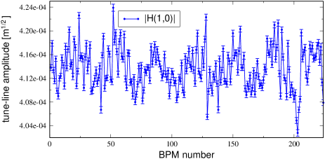
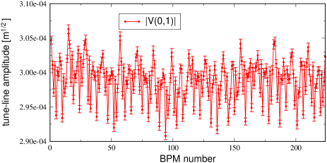
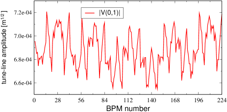
On the other hand, the amplitude of the tune lines |H(1,0)|𝐻10|H(1,0)| and |V(0,1)|𝑉01|V(0,1)| shall be constant along the ring, as indicated by the first two lines of Table 2 . There it is indeed assumed that focusing errors are already included in the model (i.e. in the beta functions used to normalize the TbT BPM data) and hence the beta-beating RDTs f2000subscript𝑓2000f_{2000} and f0020subscript𝑓0020f_{0020} of Eqs. (140)-(141) are zero. If the tune line amplitudes measured at all BPMs are not constant, three are the possible causes to be evaluated and removed prior to any further analysis involving other spectral lines.

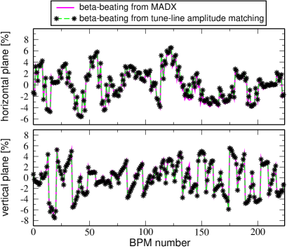
First, the linear lattice model used to evaluate the beta functions at the BPMs is incorrect. This shall result in non-zero quadrupolar RDTs f2000subscript𝑓2000f_{2000} and f2000subscript𝑓2000f_{2000}, in a modulation of the beta functions (beta-beating) and in wrong phase advances between BPMs. In Appendix C it is shown how the beta-beating is correlated to the RDTs and how to infer it from the tune line amplitudes measured at each BPM. Even if elegant and handy, such formulas are of limited applicability for several reasons: (i)𝑖(i) it is impossible to disentangle beta modulation from BPM calibration factors or tilts, (ii)𝑖𝑖(ii) quadrupoles RDTs are not measurable from the harmonic analysis of the single-BPM TbT data, (iii)𝑖𝑖𝑖(iii) second and higher order RDTs do modify the tune line amplitudes introducing a dependence on the position along the ring. Fortunately, none of these elements affects the phase of the tune line, and the difference between its value at two consecutive BPMs corresponds to the betatron phase advance. Hence by comparing and fitting the measured BPM phase advance, a reliable focusing model may be built and used to evaluate correctly the beta functions at the BPMs. As discussed in Sec. V, some octupolar CRDTs may indeed perturb the phase of the tune lines, though this effect may be controlled by a careful choice of the initial excitation (i.e. kicker strength). It is worthwhile reminding that the fit of the BPM phase advance shall be accompanied by a fit of the measured dispersion function for a reliable model.

Second, if a modulation persists even after fitting the BPM phase advance (and dispersion), it shall be verified whether second-order sextupole terms may introduce a dependence on the longitudinal position. As discussed in Appendix C, this perturbation depends on the initial oscillation amplitude (or the action), i.e. on the kicker strength, and may be evaluated from preliminary single-particle tracking simulations. For the measurement procedure discussed here, it is hence necessary to limit the kicker strength so to keep the natural modulation of the tune line amplitude induced by sextupoles well below the desired experimental resolution. This contrasts with the desire of having a large signal-to-noise ratio between spectral noise and amplitude of the sextupolar lines, which would require a strong initial excitation. Eventually a trade off shall be found with the help of tracking simulations and measured data at different kicker strengths.

The third source of tune line amplitude modulation is represented by BPM calibration factors η1𝜂1\eta\neq 1 and tilts. Assuming that the latter are negligible compared to other sources of errors, the only way to infer η𝜂\eta and remove them before carrying out the spectral analysis is to impose constant tune line amplitude at all BPMs after having verified the previous two points. The Fourier transform redone after scaling the measured data by η𝜂\eta may then be used for the analysis of the nonlinear model.

A last interesting figure to evaluate the quality of the TbT BPM data and of its harmonic analysis is represented by a cancellation condition that shall be satisfied by some measured CRDTs. According to the definitions of the normal sextupole terms of Table 2 it is straightforward to prove that

F0=2{FNS2}{FNS1}+{FNS0}0subscript𝐹02subscript𝐹𝑁𝑆2subscript𝐹𝑁𝑆1subscript𝐹𝑁𝑆00F_{0}=2\Re\{F_{NS2}\}-\Re\{F_{NS1}\}+\Re\{F_{NS0}\}\equiv 0 (7)

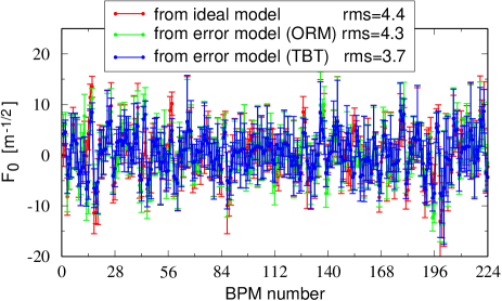
anywhere in the ring: the closer F0subscript𝐹0F_{0} is to zero, the more reliable is the harmonic analysis described here. Note that the measured F0subscript𝐹0F_{0} along the ring depends only on: (i)𝑖(i) the linear lattice model (β𝛽\beta functions used to normalize the BPM TbT data); (ii)𝑖𝑖(ii) the BPM calibration factors, spatial and spectral resolution, electronic noise and the like; (iii)𝑖𝑖𝑖(iii) initial beam excitation, i.e. kicker strength. Luckily enough, it does not depend on the nonlinear lattice model, being valid for any sextupole setting.

III.4 From normal sextupole CRDTs to sextupole errors

Let us assume to have acquired N𝑁N TbT data from NBPMsubscript𝑁𝐵𝑃𝑀N_{BPM} BPMs. From the harmonic analysis of Table 2 it is possible to infer the four normal sextupole CRDTs FNS3subscript𝐹𝑁𝑆3F_{NS3}, FNS2subscript𝐹𝑁𝑆2F_{NS2}, FNS1subscript𝐹𝑁𝑆1F_{NS1} and FNS0subscript𝐹𝑁𝑆0F_{NS0}, at all BPMs. Being these all complex quantities, a NBPM42subscript𝑁𝐵𝑃𝑀42N_{BPM}\cdot 4\cdot 2 vector \vvFNS,meas\vvsubscript𝐹𝑁𝑆𝑚𝑒𝑎𝑠\vv{F}_{NS,meas} may be defined containing the measured real and imaginary parts of the four CDRTs

\vvFNS,meas\vvsubscript𝐹𝑁𝑆𝑚𝑒𝑎𝑠\displaystyle\vv{F}_{NS,meas} =\displaystyle= ({FNS3}1,,{FNS3}NBPM,\displaystyle(\Re\{F_{NS3}\}_{1},...\ ,\Re\{F_{NS3}\}_{N_{BPM}}, (8)
{FNS3}1,,{FNS3}NBPM,\displaystyle\ \Im\{F_{NS3}\}_{1},...\ ,\Im\{F_{NS3}\}_{N_{BPM}},
,\displaystyle\ ...,
{FNS0}1,,{FNS0}NBPM).\displaystyle\ \Im\{F_{NS0}\}_{1},...\ ,\Im\{F_{NS0}\}_{N_{BPM}})\ .

An equivalent vector may be defined from the model (C-S parameters including focusing errors,β𝛽\beta and ϕitalic-ϕ\phi, and sextupole integrated gradients, K2subscript𝐾2K_{2}): The RDTs f3000subscript𝑓3000f_{3000}, f1200subscript𝑓1200f_{1200}, f1020subscript𝑓1020f_{1020}, f0120subscript𝑓0120f_{0120} and f0111subscript𝑓0111f_{0111} may be evaluated from Table 3, to be used for the evaluation of the model CRDTs through the fourth column of Table 2. Being all passages from the integrated strengths to the CRDTs linear, the model vector may be defined as

\vvFNS,mod\vvsubscript𝐹𝑁𝑆𝑚𝑜𝑑\displaystyle\vv{F}_{NS,mod} =\displaystyle= 𝐌𝐍𝐒\vvK2,subscript𝐌𝐍𝐒\vvsubscript𝐾2\displaystyle\mathbf{M_{NS}}\vv{K}_{2}\ , (9)

where \vvK2\vvsubscript𝐾2\vv{K}_{2} contains all Nsextsubscript𝑁𝑠𝑒𝑥𝑡N_{sext} known sources of sextupolar field along the ring, and 8NBPM×Nsext8subscript𝑁𝐵𝑃𝑀subscript𝑁𝑠𝑒𝑥𝑡8\cdot N_{BPM}\times N_{sext} matrix 𝐌𝐍𝐒subscript𝐌𝐍𝐒\mathbf{M_{NS}} depends on the linear lattice only, through the beta functions, the phase advances between BPMs and sextupoles and the tunes. The difference between measured and model CRDTs then reads

\vvFNS,meas\vvFNS,mod\vvsubscript𝐹𝑁𝑆𝑚𝑒𝑎𝑠\vvsubscript𝐹𝑁𝑆𝑚𝑜𝑑\displaystyle\vv{F}_{NS,meas}-\vv{F}_{NS,mod} =\displaystyle= 𝐌𝐍𝐒\vvΔK2,subscript𝐌𝐍𝐒\vvΔsubscript𝐾2\displaystyle\mathbf{M_{NS}}\vv{\Delta K}_{2}\ , (10)

where \vvΔK2\vvΔsubscript𝐾2\vv{\Delta K}_{2} contains the Nsextsubscript𝑁𝑠𝑒𝑥𝑡N_{sext} sextupole field errors to be inferred after pseudo-inverting (via SVD, for instance) the above linear system. Note how the choice of defining the CRDTs vector with the real and imaginary parts ensures the linearity of the system, whereas the choice of decomposing these complex quantities in amplitude and phases, as in Ref. Bartolini2 , would have introduced an unnecessary and avoidable nonlinearity in the problem, thus requiring a nonlinear minimization routine for the evaluation of \vvΔK2\vvΔsubscript𝐾2\vv{\Delta K}_{2}.

The linear system of Eq. (10) may be also used for the calibration of an individual sextupole. The optics model in this case is necessary for the evaluation of the (8NBPM)×18subscript𝑁𝐵𝑃𝑀1(8\cdot N_{BPM})\times 1 matrix 𝐌𝐌\mathbf{M} only, whereas the left hand side contains two CRDT vectors measured with two different sextupole strengths, i.e.

\vvFNS,meas(K2)\vvFNS,meas(K2+δK2)=𝐌𝐍𝐒δK2.\vvsubscript𝐹𝑁𝑆𝑚𝑒𝑎𝑠subscript𝐾2\vvsubscript𝐹𝑁𝑆𝑚𝑒𝑎𝑠subscript𝐾2𝛿subscript𝐾2subscript𝐌𝐍𝐒𝛿subscript𝐾2\displaystyle\vv{F}_{NS,meas}(K_{2})-\vv{F}_{NS,meas}(K_{2}+\delta K_{2})=\mathbf{M_{NS}}\delta K_{2}\ .\hskip 19.91684pt (11)

After pseudo-inverting the above system, the inferred δK2𝛿subscript𝐾2\delta K_{2} may be compared with the expected value from the change of current in the sextupole and its calibration curve. The latter may be reconstructed and compared with the magnetic model (or measurement) by repeating the procedure at different δK2𝛿subscript𝐾2\delta K_{2}. Again, the problem of calibrating a nonlinear magnetic element is reduced to a linear system when looking at the CRDTs.

III.5 From normal sextupole CRDTs to sextupole correction

The natural extension of Eq. (10) is a system for the evaluation of a sextupole corrector setting. If all sextupole magnets have independent power supplies and other sources of sextupolar fields (such as fringe fields in bending magnets) may be neglected, the pseudo-inversion of Eq. (10) provides already the set of corrections \vvδK2\vv𝛿subscript𝐾2\vv{\delta K}_{2} to insert in the sextupoles. If this is not the case and only Ncorsubscript𝑁𝑐𝑜𝑟N_{cor} corrector sextupoles are available (which is the case at the ESRF storage rings, with 224 sextupoles grouped in 7 families and only 12 sextupole correctors available), the system then reads

\vvFNS,meas\vvFNS,ref\vvsubscript𝐹𝑁𝑆𝑚𝑒𝑎𝑠\vvsubscript𝐹𝑁𝑆𝑟𝑒𝑓\displaystyle\vv{F}_{NS,meas}-\vv{F}_{NS,ref} =\displaystyle= 𝐌𝐍𝐒,𝐜𝐨𝐫\vvK2cor,subscript𝐌𝐍𝐒𝐜𝐨𝐫\vvsuperscriptsubscript𝐾2𝑐𝑜𝑟\displaystyle\mathbf{M_{NS,cor}}\vv{K}_{2}^{cor}\ , (12)

where \vvK2cor\vvsuperscriptsubscript𝐾2𝑐𝑜𝑟\vv{K}_{2}^{cor} contains the strengths of the Ncorsubscript𝑁𝑐𝑜𝑟N_{cor} sextupole correctors to be evaluated after pseudo-inverting the above system, and the 8NBPM×Ncor8subscript𝑁𝐵𝑃𝑀subscript𝑁𝑐𝑜𝑟8\cdot N_{BPM}\times N_{cor} matrix 𝐌𝐍𝐒,𝐜𝐨𝐫subscript𝐌𝐍𝐒𝐜𝐨𝐫\mathbf{M_{NS,cor}} depends on the beta functions and the phase advances between BPMs and the correctors. Note that \vvFNS,ref\vvsubscript𝐹𝑁𝑆𝑟𝑒𝑓\vv{F}_{NS,ref} (reference or desired vector) has been used in place of \vvFNS,mod\vvsubscript𝐹𝑁𝑆𝑚𝑜𝑑\vv{F}_{NS,mod} (model vector). The difference may be of importance for those machines (like the ESRF storage ring) where beta-beating is corrected up to some percents and special insertion optics break up significantly the machine natural periodicity. \vvFNS,ref\vvsubscript𝐹𝑁𝑆𝑟𝑒𝑓\vv{F}_{NS,ref} may refer hence to the ideal lattice without any insertion optics, whereas \vvFNS,mod\vvsubscript𝐹𝑁𝑆𝑚𝑜𝑑\vv{F}_{NS,mod} refers to the actual model including insertion optics (if any) and all known lattice errors. It is assumed here that the best CRDT correction shall be based on the ideal vector \vvFNS,ref\vvsubscript𝐹𝑁𝑆𝑟𝑒𝑓\vv{F}_{NS,ref}, rather than on \vvFNS,mod\vvsubscript𝐹𝑁𝑆𝑚𝑜𝑑\vv{F}_{NS,mod}. Once more, the problem of correcting nonlinear magnetic elements is reduced to a linear system, Eq. (12), to be pseudo-inverted.

III.6 From skew sextupole CRDTs to sextupole tilts

The procedure described in Sec. III.5 may be repeated, with some precautions, for the evaluation of sextupole tilts. From the harmonic analysis of the TbT BPM data and Table 2 it is possible to infer the four skew sextupole CRDTs FSS3subscript𝐹𝑆𝑆3F_{SS3}, FSS2subscript𝐹𝑆𝑆2F_{SS2}, FSS1subscript𝐹𝑆𝑆1F_{SS1} and FSS0subscript𝐹𝑆𝑆0F_{SS0}, at all BPMs, and cast them in a NBPM42subscript𝑁𝐵𝑃𝑀42N_{BPM}\cdot 4\cdot 2 vector \vvFSS,meas\vvsubscript𝐹𝑆𝑆𝑚𝑒𝑎𝑠\vv{F}_{SS,meas}

\vvFSS,meas\vvsubscript𝐹𝑆𝑆𝑚𝑒𝑎𝑠\displaystyle\vv{F}_{SS,meas} =\displaystyle= ({FSS3}1,,{FSS3}NBPM,\displaystyle(\Re\{F_{SS3}\}_{1},...\ ,\Re\{F_{SS3}\}_{N_{BPM}}, (13)
{FSS3}1,,{FSS3}NBPM,\displaystyle\ \Im\{F_{SS3}\}_{1},...\ ,\Im\{F_{SS3}\}_{N_{BPM}},
,\displaystyle\ ...,
{FSS0}1,,{FSS0}NBPM).\displaystyle\ \Im\{F_{SS0}\}_{1},...\ ,\Im\{F_{SS0}\}_{N_{BPM}})\ .

The evaluation of the corresponding vector from the model require a preliminary step. As discussed in Sec. III.2, contrary to normal sextupole terms, it is not possible to ignore the second-order contribution to the skew sextupole CRDTs due to cross-terms between coupling and normal sextupole RDTs, see Eq. (3). In other words, ideal skew sextupoles CRDTs shall all be zero, but even with perfectly upright sextupoles they may be nonzero because any residual coupling in the machine transfers normal sextupole spectral harmonics in the other plane, hence generating skew sextupole harmonics and corresponding CRDTs. Not taking into account this natural contribution would corrupt the evaluation of sextupole tilts. For this reason new analytic formulas valid to second order have been derived. They are presented in Appendix A and shall be used for the evaluation of the skew sextupole ORDTs gjklmsubscript𝑔𝑗𝑘𝑙𝑚g_{jklm}, and hence of the CRDTs FSSsubscript𝐹𝑆𝑆F_{SS}. Provided that betatron coupling is well modelled, the second-order contribution to the CRDTs FSSsubscript𝐹𝑆𝑆F_{SS} may be then computed and any difference between the model vector \vvFSS,mod\vvsubscript𝐹𝑆𝑆𝑚𝑜𝑑\vv{F}_{SS,mod} and the measured one \vvFSS,meas\vvsubscript𝐹𝑆𝑆𝑚𝑒𝑎𝑠\vv{F}_{SS,meas} will depend on the sextupole tilts only, i.e.

\vvFSS,meas\vvFSS,mod\vvsubscript𝐹𝑆𝑆𝑚𝑒𝑎𝑠\vvsubscript𝐹𝑆𝑆𝑚𝑜𝑑\displaystyle\vv{F}_{SS,meas}-\vv{F}_{SS,mod} =\displaystyle= 𝐌𝐒𝐒\vvJ2,subscript𝐌𝐒𝐒\vvsubscript𝐽2\displaystyle\mathbf{M_{SS}}\vv{J}_{2}\ , (14)

where the angles θ𝜃\theta can be extracted from J2subscript𝐽2J_{2} according to

θ=13arcsin(J2K2),𝜃13subscript𝐽2subscript𝐾2\displaystyle\theta=-\frac{1}{3}\arcsin{\left(\frac{J_{2}}{K_{2}}\right)}\ , (15)

since the skew sextupole strength introduced by a tilted sextupole is J2=K2sin(3θ)subscript𝐽2subscript𝐾23𝜃J_{2}=-K_{2}\sin{(3\theta)}.

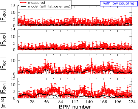
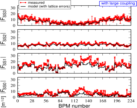
It is worthwhile mentioning that measuring skew sextupolar CRDTs will be unavoidably more difficult than extracting normal sextupole CRDTs, the latter scaling with the (strong) sextupole gradients, while the former scale with the (small) sextupole tilts. Depending on the lattice configuration and coupling correction, \vvFSS\vvsubscript𝐹𝑆𝑆\vv{F}_{SS} may be one or two orders of magnitude lower than \vvFNS\vvsubscript𝐹𝑁𝑆\vv{F}_{NS}.

In machine with skew sextupole correctors, the system of Eq. (12) may be modified as

\vvFSS,meas\vvsubscript𝐹𝑆𝑆𝑚𝑒𝑎𝑠\displaystyle\vv{F}_{SS,meas} =\displaystyle= 𝐌𝐒𝐒,𝐜𝐨𝐫\vvJ2cor,subscript𝐌𝐒𝐒𝐜𝐨𝐫\vvsuperscriptsubscript𝐽2𝑐𝑜𝑟\displaystyle-\mathbf{M_{SS,cor}}\vv{J}_{2}^{cor}\ , (16)

where the reference vector \vvFSS,ref\vvsubscript𝐹𝑆𝑆𝑟𝑒𝑓\vv{F}_{SS,ref} in this case is zero. In machine without skew sextupole correction, skew quadrupoles may be used to correct, along with coupling, skew sextupole CRDTs, via the second-order contributions fjklm(2)superscriptsubscript𝑓𝑗𝑘𝑙𝑚2f_{jklm}^{(2)}. This later option, however, would require to solve a more complex (but still linear in the skew quadrupole strengths) system not discussed here.

IV Experimental results

IV.1 Preparing measurements

The TbT acquisition of the commercial Libera-Brilliance BPMs installed in the ESRF storage ring requires some care in its preparation. Even though the measurement is rather quick, a series of machine studies were carried out between 2010 and 2011 for the correct setup.

First of all, in the case of the ESRF storage ring the ideal beam filling pattern is the 1/3, i.e. with a train of about 330 bunches separated by about 660 empty RF buckets. The interest of this pattern is threefold. First, it allows a straightforward synchronization among all 224 BPMs and the bunch train, by using the booster (whose circumference is exactly 1/3 the one of the storage ring) and fast monitors in the transfer line. Second, both the horizontal and the vertical kickers may by synchronized so to have the bunch train on their flattop: The measured invariants and CRDTs would be corrupted if part of the beam experiences the kicker pulse rise and/or fall. Third, this filling mode maximizes the BPM resolution, the beam signal being integrated over 1/3 of the revolution frequency, whereas a few-bunch pattern would provide intense peak signal with a noisier integrated value.

Another parameter to be adjusted to minimize the BPM noise and to prevent a saturation of the signal (and hence a corrupted harmonic analysis) is the beam current against the amplification factor of the acquisition system. In order to have the best dynamic range from a few μ𝜇\muA to 200 mA, the ESRF BPMs apply a variable signal amplification. The special optics implemented for this measurement with almost zero linear chromaticity and amplitude dependent detuning may sustain up to 10 mA before losing the beam. However, in order to maximize the BPM resolution during the signal digitization, measurements are carried out with 7 mA for a kicker excitation so to displace horizontally the beam from 1.3 to 5.5 mm. With a β𝛽\beta function of 36.6 m this corresponds to an invariant between about 104superscript10410^{-4} and 4×1044superscript1044\times 10^{-4} m1/2. Higher beam current would result in a different amplification range with lower digitization resolution, whereas stronger excitations risk to saturate the BPM signal.

As mentioned in Sec. III.3 the kicker strengths shall be a trade-off between spectral resolution (the stronger, the better) and second-order terms affecting the invariance of the tune line amplitude (the weaker, the better). Measurements are usually repeated at different kicker strengths. For the final analysis of sextupolar CRDTs only the data set of 50 repeated measurements with both invariants 2.0×10⁴similar-to-or-equalsabsent2.0superscript104\simeq 2.0\times 10^{-4} m1/2 is used (corresponding to displacement of about 2.5 mm horizontally and 1.0 mm vertically, with β𝛽\beta functions of 36.6 and 6.0 m). For the octupolar model, instead, data with stronger excitations are used. Note that hereafter, unless specified otherwise, the invariant is referred to as 1/22I122𝐼1/2\sqrt{2I} so to be equal to the tune line amplitude (see first two rows in Table 2).

As discussed in Sec. II, even though more than 2000 turns may be stored by the BPMs and the weak decoherence ensures about 1000 turns of exploitable data, it will be shown how the best results are obtained when only 256 turns are used for the analysis of sextupolar CRDTs (512 turns for the octupolar).

IV.2 Linear analysis of TbT BPM data
Refer to caption

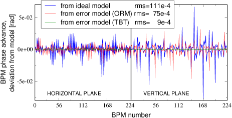
Figure 2: (Color) Example of measured BPM phase advance deviation from the models: ideal (blue), with errors inferred from ORM measurement (red) and with errors after fitting the measured BPM phase advance and dispersion (green). Data correspond to the fifth row of Table 4

Refer to caption

Refer to caption

Figure 3: (Color) Example of measured variation of the horizontal (top) and vertical (bottom) tune-line amplitudes along the ESRF storage ring. Data correspond to the last row of Table 4 (average over 50 acquisitions).

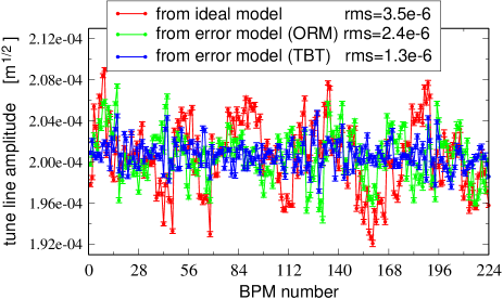
The starting linear optics model used to evaluate the expected CRDTs and the β𝛽\beta functions at the BPMs (necessary for the construction of TbT signals to be analyzed x~(N)=x(N)/βx~𝑥𝑁𝑥𝑁subscript𝛽𝑥\tilde{x}(N)=x(N)/\sqrt{\beta_{x}} and y~(N)=y(N)/βy~𝑦𝑁𝑦𝑁subscript𝛽𝑦\tilde{y}(N)=y(N)/\sqrt{\beta_{y}}) is based on the preliminary measurement and fit of the orbit response matrix (ORM) and dispersion prstab_esr_coupling . To this end, only quadrupole and dipole relative errors are introduced, with a cutoff in the fit so not to overcome the specifications of 103superscript10310^{-3} for the quadrupoles. No other source of errors is introduced at this stage. As figure of merit to assess the quality of the linear lattice model, the BPM phase advances are used: The smaller the deviation from the theoretical values, the better the model. The BPM phase is nothing else than the phase of the tune line (i.e. the first harmonic of the FFT of the TbT data) plus an arbitrary initial phase which depends on the trigger of the acquisition system. Assuming that all BPMs are well synchronized, the difference between the tune phases at two monitors shall correspond to the BPM phase advance, the arbitrary phase being canceled out. At each pair of BPMs along the ring, the difference between measured and model phase advances may be evaluated and plotted. Its root-mean-square (rms) value over all BPMs may be also computed and used as single figure of merit. In Fig. 3 an example is shown. If the ideal model without errors is used, large deviations are observed, with an rms of about 11 mrad. When the linear error model computed from the standard ORM measurement is used, the residual rms drops to about 7.5 mrad, with some remaining spikes in the vertical plane. On top of the ORM model, a response matrix on the BPM phase advance and dispersion was built and applied to the measured values to further reduce the deviation with the measured data. Indeed alternative models may be defined so to have a residual rms deviation below 1 mrad. It is interesting to note how when going from the ideal model, to the one from the ORM, until the one(s) matching the measured BPM phase advances, the rms variation along the ring of the tune line amplitude, i.e. of the invariant, is also reduced, as displayed in Table 4.

Table 4: Kicker strengths and corresponding invariants for the 8 sets of TbT BPM data (50 repeated acquisitions). The rms modulation of the tune line amplitude (i.e. of the invariant) and the rms deviation from the model BPM phase advance are measured with three different linear lattice models: ideal with no error, with errors inferred from precedent ORM measurement and fit, and from the harmonic analysis of TbT data. Horizontal and vertical data for the BPM phase advance are merged together when computing the rms deviation.
        ideal lattice model    model with errors (ORM)    model with errors (TbT)
(H,V)
kicker
strength
(A, kV)
(H,V) mean
invariant
(m1/2)
×104absentsuperscript104\times 10^{-4}
(H,V) rms
err. invariant
(m1/2)
×106absentsuperscript106\times 10^{-6}
BPM
phase advance
rms error
×104absentsuperscript104\times 10^{-4}(rad)
(H,V) rms
err. invariant
(m1/2)
×106absentsuperscript106\times 10^{-6}
BPM
phase advance
rms error
×104absentsuperscript104\times 10^{-4}(rad)
(H,V) rms
err. invariant
(m1/2)
×106absentsuperscript106\times 10^{-6}
BPM
phase advance
rms error
×104absentsuperscript104\times 10^{-4}(rad)
 (  50, 1.0 )  ( 0.52, 0.89 ) ( 0.9, 1.6 ) 111 ( 0.7, 1.0 ) 75 ( 0.4, 0.4 ) 16
 ( 100, 1.0 )  ( 1.00, 0.90 ) ( 1.7, 1.6 ) 110 ( 1.3, 1.0 ) 74 ( 0.7, 0.4 ) 13
 ( 100, 1.5 )  ( 1.00, 1.37 ) ( 1.8, 2.4 ) 110 ( 1.3, 1.5 ) 74 ( 0.7, 0.7 ) 14
 ( 200, 1.5 )  ( 1.99, 1.42 ) ( 3.5, 2.5 ) 111 ( 2.4, 1.6 ) 76 ( 1.4, 0.6 ) 11
 ( 200, 2.1 )  ( 2.01, 1.98 ) ( 3.5, 3.5 ) 111 ( 2.4, 2.3 ) 75 ( 1.3, 0.9 )  9
 ( 250, 2.7 )  ( 2.55, 2.58 ) ( 4.5, 4.5 ) 111 ( 3.0, 3.3 ) 77 ( 1.7, 1.5 ) 12
 ( 400, 2.5 )  ( 4.11, 2.52 ) ( 7.5, 4.8 ) 119 ( 4.8, 4.0 ) 91 ( 3.3, 2.2 ) 35
 ( 400, 3.0 )  ( 4.14, 2.98 ) ( 7.5, 6.0 ) 118 ( 4.8, 5.0 ) 91 ( 3.5, 3.0 ) 36

It is also worthwhile noticing how the residual rms error on the BPM phase advance has a minimum for the fifth data set of Table 4, with a kicker excitation so to generate an invariant of about 2×1042superscript1042\times 10^{-4} m1/2. Larger excitations seem to induce greater errors that could not be correlated to linear lattice elements. Octupolar terms affecting the tune lines may be the source of this larger discrepancy.

Refer to caption


Figure 4: (Color) Example of measured horizontal tune line amplitude (i.e. invariant) modulation along the ESRF ring when using different lattice models: ideal (blue), with errors inferred from ORM measurement (red) and from TbT data plus dispersion (green). Rms values correspond to the fifth row of Table 4

As far as the tune line amplitude variation along the ring is concerned, all data set with excitation lower than 2.6×1042.6superscript1042.6\times 10^{-4} m1/2 show a modulation below 1%percent11\% (with the TbT model). According to tracking simulation results of Table 16, second-order sextupolar terms contribute for a fraction of this modulation only. When comparing modulation observed in single-particle tracking (Fig. 28) and that measured with the strongest excitation (Fig. 3), even though a similar pattern may be guessed in the horizontal plane, the fast modulation observed in the vertical plane is unexpected. This indeed can be explained by small differences in the signal attenuation induced by BPM cables of different lengths (an effect visible in the sum BPM signal). For sake of completion effective BPM gains have been computed so to cancel the tune line amplitude modulation corresponding to the fifth data set of Table 4, though they turned out to play a limited role in the nonlinear analysis.

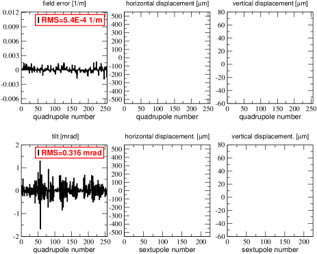
A brief digression on the effective linear lattice model inferred from the the BPM phase advance (and dispersion) response matrix is worth to be introduced. The matrix has been built having different error sources: besides quadrupole field errors and rotation (for coupling), quadrupole and sextupole displacements (longitudinal, horizontal and vertical) have been introduced along with longitudinal dislocations of BPMs. It turned out that longitudinal displacements have a negligible impact on the BPM phase advances, whereas this is not the case for the other two axes. The best SVD fit was obtained with the error model displayed in the centre plot of Fig. 6. The corresponding rms values are compatible with specifications and well within the results from survey measurements NoteSurvey . Such a model, however, is difficult to handle, because magnet displacement would require the distorted orbit to be taken into account, complicating the overall analysis. Nevertheless, the same SVD fit could be obtained with quadrupole field errors only, at the price of increasing unrealistically their values, well above their specifications (bottom plot of Fig. 6). Nonetheless, this has the advantage of not introducing any complication with the orbit and large quadrupole errors are to be considered as representative of the sextupole displacement too. The nonlinear analysis discussed in the next section is based on this later baseline linear model.
Refer to caption

Figure 5: (Color) Example of measured F0subscript𝐹0F_{0} along the ESRF storage ring when different linear models (β𝛽\beta functions at BPMs) are used: ideal lattice(blue), with errors inferred from ORM measurement (red) and TbT data plus dispersion (green). Data correspond to the fifth row of Table 4 (average over 50 acquisitions).

Refer to caption

Refer to caption

Refer to caption

Figure 6: (Color) Top: lattice error model inferred from ORM measurement with quadrupole errors only (dipole errors are not displayed here), BPM phase advance rms error of 7.5 mrad. Centre: lattice error model with magnet displacements (rms error 0.9 mrad). Bottom: lattice model with equivalent rms error of 0.9 mrad, but (large) quadrupole errors only.

Even though not used for the determination of linear lattice model, it is interesting to note how the CRDTs cancellation condition defined by F0subscript𝐹0F_{0} of Eq. (7) is improved when the BPM phase advance is corrected. In general, the closer F0subscript𝐹0F_{0} is to zero among all BPMs, the more accurate is the harmonic analysis. F0subscript𝐹0F_{0} is evaluated with the CRDTs measured from the sextupolar spectral lines according to Table 2. Its rms values (for the fifth data set of Table 4) goes from 4.4 m-1/2 with the ideal linear model, to 4.3 m-1/2 with the ORM error model, and eventually to 3.2 m-1/2 with the model based on the BPM phase advance, even though large fluctuations among the 50 acquisitions are present, as shown in Fig. 5.

In conclusion, the linear analysis of the tune line (amplitude and phase) provided an effective linear model that improves considerably the quality of the harmonic analysis. The deviation between model and measured BPM phase advance is reduced by a factor greater than ten. The modulation of the tune line (i.e. of the invariant) is reduced from 2%percent22\% to less than 1%percent11\%. The cancellation term F0subscript𝐹0F_{0} is reduced by about 20%percent2020\%. Effective BPM gains could be inferred from the tune line amplitude modulation.

IV.3 Nonlinear analysis of TbT BPM data

Refer to caption

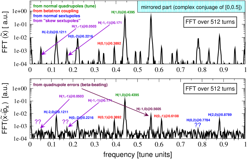
Figure 7: (Color) Example of horizontal (left) and vertical (right) spectral lines inferred from the FFT of TbT BPM data measured after exciting transversely the beam with the strongest kicker strengths of Table 5. A special sextupole setting was used to reduce detuning with amplitude and chromaticity and to enhance the normal sextupole spectral lines. Higher-order octupolar-like lines (in maroon) are also excited and measurable, though they may overlap the sextupolar-like, corrupting the CRDTs measurement and resulting in large F0subscript𝐹0F_{0}.

Refer to caption       Refer to caption

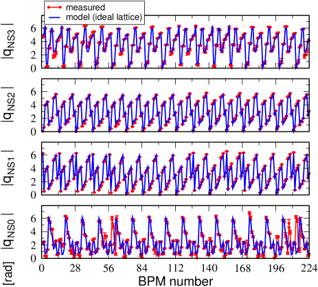
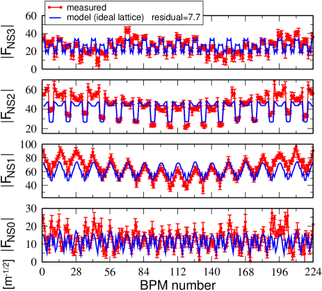
Figure 8: (Color) Red: CRDT phases (left) and amplitudes (right) measured at the ESRF storage ring (with a special dedicated optics). Blue: the same quantities computed from the ideal perfect lattice. The residual for this model is =7.77.7\mathcal{R}=7.7 m-1/2.
Table 5: Measured rms variation along the ESRF storage ring of F0subscript𝐹0F_{0} against different lattice models (i.e. β𝛽\beta functions at BPMs) for all acquired data sets. The mean value is between -0.4 and 0.8 depending on the set (50 acquisition each, FFT over 256 turns).
      rms F0subscript𝐹0F_{0} (m-1/2)
(H,V)
kicker
strength
(A, kV)
(H,V) mean
invariant
m1/2
×104absentsuperscript104\times 10^{-4}
ideal
lattice
model
error
model
(ORM)
error
model
(SVD)
 (  50, 1.0 )  ( 0.52, 0.89 ) 8.4 8.8 8.5
 ( 100, 1.0 )  ( 1.00, 0.90 ) 5.6 5.9 5.4
 ( 100, 1.5 )  ( 1.00, 1.37 ) 4.8 5.0 4.4
 ( 200, 1.5 )  ( 1.99, 1.42 ) 4.4 4.4 3.9
 ( 200, 2.1 )  ( 2.01, 1.98 ) 4.4 4.3 3.7
 ( 250, 2.7 )  ( 2.55, 2.58 ) 5.1 4.9 4.3
 ( 400, 2.5 )  ( 4.11, 2.52 ) 7.8 7.5 7.5
 ( 400, 3.0 )  ( 4.14, 2.98 ) 7.9 7.6 7.6

The effective linear lattice error model discussed in the previous section may now be used to evaluate the modulated C-S parameters necessary to normalize the TbT data (β𝛽\beta functions) and to evaluate the model CRDTs from Tables 3 and 2. The measured CRDTs are instead inferred from the sextupolar lines H(2,0)𝐻20H(-2,0), H(0,2)𝐻02H(0,-2) and V(±1,1)𝑉plus-or-minus11V(\pm 1,-1) according to Table 2. These lines are represented in blue in the example of measured spectra of Fig. 7. As for the linear analysis, a data set among those acquired at different kicker strengths is to be chosen, considering that a too weak excitation may affect the measurement because of the low signal-to-noise ratio, whereas a too strong excitation may introduce high-order terms not included in the present analysis. As discussed in Sec. III.3, the nonlinear analysis presented here is valid as long as the CRDT residual F0subscript𝐹0F_{0} of Eq. (7) is much lower than the average CRDT amplitudes. The rms values of F0subscript𝐹0F_{0} (computed after averaging among the 224 BPMs and the 50 acquisitions) for each data set and for different linear lattice models are reported in Table 5. Because of the ESRF storage ring tune working point (Qx=36.440subscript𝑄𝑥36.440Q_{x}=36.440 and Qy=13.390subscript𝑄𝑦13.390Q_{y}=13.390) two sextupolar lines, H(0,2)𝐻02H(0,-2) and V(1,1)𝑉11V(-1,-1), necessary for the evaluation of as many CRDTs receive a contribution from higher-order octupolar terms, as shown in Fig. 7. A complete list of the octupolar spectral lines may be found in Ref. Bartolini1 . If not taken into account or avoided, this superposition will corrupt the CRDT measurement and the overall nonlinear model. Even though it is not possible to disentangle the individual contributions, the CRDT residual F0subscript𝐹0F_{0} may be evaluated: the closer to zero, the less detrimental are the octupolar-like terms. Another way out may be found by slightly detuning the machine so to ensure a sufficient separation between these lines: By setting for example Qx=36.438subscript𝑄𝑥36.438Q_{x}=36.438 and Qy=13.385subscript𝑄𝑦13.385Q_{y}=13.385 a separation of 0.022 in tune units would be assured. In the acquired data (at nominal tunes) the mean value of F0subscript𝐹0F_{0} is always very close to zero (between -0.4 and 0.8 m-1/2, depending on the data set). The lowest rms F0subscript𝐹0F_{0} (3.7 m-1/2) is obtained for an excitation corresponding to a mean invariant (in both planes) of 2.0×1042.0superscript1042.0\times 10^{-4} m1/2. The CRDTs measured from this data set are then used for the nonlinear lattice modelling.
Refer to caption       Refer to caption

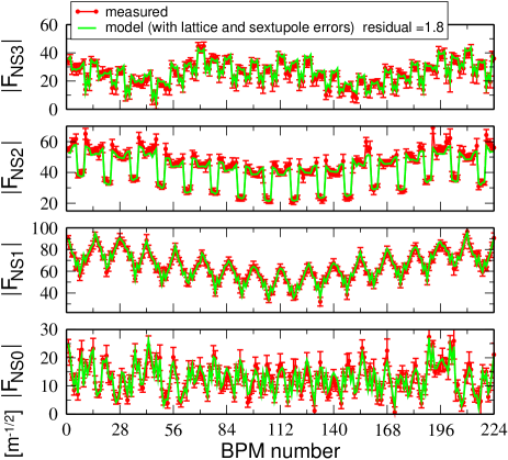
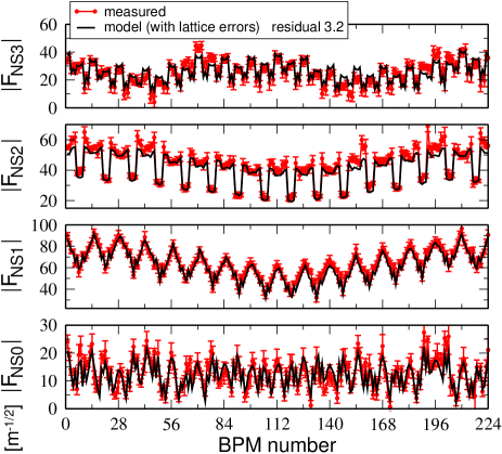
Figure 9: (Color) Amplitudes of normal sextupole CRDTs (red curves) measured at the ESRF storage ring (with a special dedicated optics). Left: comparison with the model curves obtained from the lattice model comprising ideal sextupoles and focusing errors and coupling (residual =3.23.2\mathcal{R}=3.2 m-1/2). Right: comparison with the the same linear model after introducing sextupole errors and sextupolar components in the main bending magnets (=1.81.8\mathcal{R}=1.8 m-1/2).

As for the linear analysis, a figure of merit needs to be defined to quantify the goodness of the sextupole model. The difference between the measured CRDT vector and the one for model may be used to this end. The rms value of this vector, i.e. the residual \mathcal{R}, provides a figure of merit for the model,

residual residual \displaystyle\hbox{residual\ }\mathcal{R} =\displaystyle= <|\vvFNS,meas\vvFNS,mod|2>absentsuperscript\vvsubscript𝐹𝑁𝑆𝑚𝑒𝑎𝑠\vvsubscript𝐹𝑁𝑆𝑚𝑜𝑑2absent\displaystyle\sqrt{<|\vv{F}_{NS,meas}-\vv{F}_{NS,mod}|^{2}>}
=\displaystyle= 1Ni=1N(FNS,meas(i)FNS,mod(i))2,1𝑁superscriptsubscript𝑖1𝑁superscriptsubscript𝐹𝑁𝑆𝑚𝑒𝑎𝑠𝑖subscript𝐹𝑁𝑆𝑚𝑜𝑑𝑖2\displaystyle\sqrt{\frac{1}{N}\sum_{i=1}^{N}{(F_{NS,meas}(i)-F_{NS,mod}(i))^{2}}}\ ,

where N=8NBPM𝑁8subscript𝑁𝐵𝑃𝑀N=8\cdot N_{BPM} (the 4 CRDTs are complex quantities, separated in real and imaginary parts, see Eq. (8)). It is worthwhile noticing that \mathcal{R} depends greatly on the lattice: Different machines and optics may result in different residuals for a similarly good sextupole model. In order to compare different storage rings or settings, the residual may be normalized by the mean CRDT amplitude.

A convenient way to display measured and model CRDTs is to separate their phase and amplitude. In the left plot of Fig. 8 the measured CRDT phases are shown together with the corresponding expectation from the ideal model of the ESRF storage ring. The agreement is already remarkable, as are the small statistical error bars. When comparing the CRDT amplitude instead (right plot of Fig. 8), the 16-fold periodicity of the ideal curves is modulated in the measured CRDTs. The overall residual is =7.77.7\mathcal{R}=7.7 m-1/2.

Interestingly, in an earlier analysis based on a sextupole calibration curve measured in 2001 the initial residual was about 10%percent1010\% higher (=8.48.4\mathcal{R}=8.4 m-1/2) and the magnetic errors inferred from the measured CRTDs yielded suspiciously large errors in some sextupole families. This curve was indeed obtained after cycling a spare sextupole to 250 A. On the other hand, those installed in the ring (mechanically and magnetically identical to the spare one, with a few exceptions) are grouped in seven families (3 chromatic and 4 harmonic) subjected to different cyclings: close to 250 A for the chromatic sextupoles, between 120 and 150 A for the harmonics. These facts triggered a new campaign of magnetic measurements in 2012, reproducing in the laboratory the different cyclings. These new calibration curves are used since then for this analysis, resulting in the smaller initial residual of =7.77.7\mathcal{R}=7.7 m-1/2 and in much lower errors in the harmonic sextupoles. This was the first evidence of the predicting power of this new technique.

The observed modulation of the CRDT amplitudes on top of the 16-fold periodicity is greatly reproduced after introducing in the model the linear lattice errors, as shown in the left plot of Fig. 9. The modulated β𝛽\beta functions and phase advances seem to be an important source, the residual \mathcal{R} dropping by more than 60%percent6060\% to 3.2 m-1/2. It should be mentioned that the ESRF storage ring suffers from large β𝛽\beta beating (about 23%2percent32-3\% rms) compared to more recent third generation light sources (well below 1%percent11\%), because only 32 corrector quadrupoles are available for its correction (out of 256 magnets grouped in 6 families). The modulation of the CRDT amplitudes in other machines, then, shall depend greatly on their level of β𝛽\beta beating. As far as the ESRF storage ring is concerned, this second-order effect of quadrupole errors on sextupole resonances generates in some regions CRDTs about 50%percent5050\% (up to 100%percent100100\% for the vertical CRDT FNS0subscript𝐹𝑁𝑆0F_{NS0}) larger than in an ideal machine (see right plot of Fig. 8). This may have a considerable impact on the dynamic aperture of the ring (the larger the CRDTs, the greater the phase space distortion), independently on any possible sextupole error.

Before performing the SVD pseudo-inversion of the linear system of Eq. (10) to infer sextupole errors, the measured CRDTs are compared to the model after introducing sextupolar fields in the 64 main bending magnets. Measurements performed on prototypes in the early 90s Laurent-MeasurDipoles indicated an integrated sextupole field of 1.8±0.1plus-or-minus1.80.1-1.8\pm 0.1 T/m. The plot of Fig. 10 shows how the residual \mathcal{R} reaches a minimum with a field of 1.77±0.09plus-or-minus1.770.09-1.77\pm 0.09 T/m, The agreement is excellent, again confirming the reliability of this measurement. Interestingly, when solving the system of Eq. (10) to evaluate the sextupole errors, the average error per family is reduced by about one order of magnitude after introducing the -1.77 T/m sextupole field in all 64 bending magnets, as reported in Table 6.
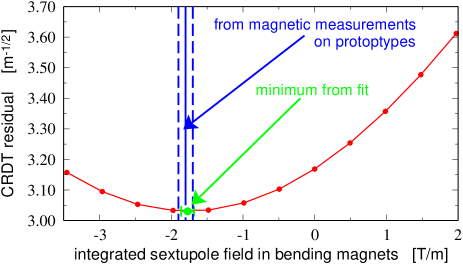
Refer to caption

Figure 10: (Color) Dependence of the residual \mathcal{R} on the sextupolar component in bending magnets, where the blue line indicates the field measured on two prototypes. The residual is computed before introducing errors in the 224 sextupoles.

Table 6: Mean and rms relative sextupole field errors (per family) inferred from the CRDTs measurement. The first column corresponds to the bare machine, whereas the second column is obtained after inserting a sextupole field in the main 64 bending magnets. This improves the overall residual \mathcal{R} (see Fig. 10) and lowers the average errors in the 224 sextupoles by about one order of magnitude.
relative error [%percent\%] (average ±plus-or-minus\pm rms) per family
   family   with baseline   with -1.77 T/m
  model   in bendings
S4 -0.12 ±plus-or-minus\pm 0.79 -0.02  ±plus-or-minus\pm 0.80
S6  0.20 ±plus-or-minus\pm 0.43 -0.02  ±plus-or-minus\pm 0.43
S13 -0.14 ±plus-or-minus\pm 0.34  0.02  ±plus-or-minus\pm 0.34
S19  0.04 ±plus-or-minus\pm 0.11 similar-to\sim0.0 ±plus-or-minus\pm 0.11
S20 -0.07 ±plus-or-minus\pm 0.11  0.01  ±plus-or-minus\pm 0.11
S22  0.24 ±plus-or-minus\pm 0.41 -0.03  ±plus-or-minus\pm 0.41
S24 -0.09 ±plus-or-minus\pm 0.41  0.01  ±plus-or-minus\pm 0.42

However, in both cases the sextupole family S4 seems to have a larger rms spread (0.8%percent0.80.8\%) compared to other families (between 0.1%percent0.10.1\% and 0.4%percent0.40.4\%). The magnets exhibiting the largest deviations turned out to be the only four (recently installed) independent sextupoles, with a relative error of about 1.5%percent1.5-1.5\%. These are shorter than the standard ones (20 cm instead of 40 cm) and have been displaced by 10 cm with respect to the nominal position so to lengthen two straight sections. New positions and calibration curves have been included in the model (the integrated strength shall be the same of the standard S4 sextupoles). A more detailed analysis on these magnets is reported in Sec. IV.5. When introducing the sextupole field in the bending magnets and fitting the 224 magnet errors by inverting the system of Eq. (10), the residual drops to =1.81.8\mathcal{R}=1.8 m-1/2: The corresponding CRDT amplitudes are displayed in the right plot of Fig. 9, while the errors (mean and rms of each family) are reported in the last column of Table 6: The great majority of the sextupole errors is well below the ±1%plus-or-minuspercent1\pm 1\% specification, as displayed in Fig. 11.

Of course, results vary according to the parameters for the SVD pseudo-inversion of Eq. (10). All the results shown in this section are derived by cutting the number of eigen-vectors to 26 (out of 224): more vectors induce a limited reduction of less than 0.1 m-1/2 in the final residual \mathcal{R} at the expenses of large sextupole errors, well beyond 1%percent11\%.

Refer to caption

Figure 11: (Color) Errors in the 224 sextupoles as computed from the (SVD) pseudo-inversion of the system in Eq. (10). Quality specifications for those magnets are at ±1%plus-or-minuspercent1\pm 1\%. The SVD is performed with 26 (out of 220) eigen-values and sextupoles are assumed to be perfectly positioned longitudinally. The residual with this set is =1.81.8\mathcal{R}=1.8 m-1/2. For each family, mean and rms errors are reported in the last column of Table 6.

The sextupole field errors of Fig. 11 are computed assuming that all 224 sextupoles are placed at their nominal longitudinal position along the ring. Any displacement along s𝑠s, e.g. the circumference, would change the CRDTs through the β𝛽\beta functions and phases ϕitalic-ϕ\phi (see Table 3) because of the dependence of the latter on s𝑠s. Part of the field errors attributed to the magnets by the CRDTs may actually be a combination of magnetic imperfection and longitudinal displacement. Periodic metrological surveys and adjustments are carried out at the ESRF storage ring twice per year. However, they ensure a state-of-the-art alignment on the transverse plane only. A longitudinal alignment was carried out in the early 90s during the installation only, with an accuracy estimated in the mm range. To understand the contribution of longitudinal displacements δs𝛿𝑠\delta s on the CRDTs and, hence, on the equivalent field errors in the sextupole, the response matrix of Eq. (10) was extended, namely

\vvFNS,meas\vvFNS,mod\vvsubscript𝐹𝑁𝑆𝑚𝑒𝑎𝑠\vvsubscript𝐹𝑁𝑆𝑚𝑜𝑑\displaystyle\vv{F}_{NS,meas}-\vv{F}_{NS,mod} =\displaystyle= 𝐌𝐍𝐒(wK\vvδK2ws\vvδs),subscript𝐌𝐍𝐒subscript𝑤𝐾\vv𝛿subscript𝐾2subscript𝑤𝑠\vv𝛿𝑠\displaystyle\mathbf{M_{NS}}\left(\begin{array}[]{c}w_{K}\cdot\vv{\delta K}_{2}\\ w_{s}\cdot\vv{\delta s}\end{array}\right)\ , (20)

where \vvδs\vv𝛿𝑠\vv{\delta s} contains the Nsext=224subscript𝑁𝑠𝑒𝑥𝑡224N_{sext}=224 sextupole longitudinal displacements, whereas wKsubscript𝑤𝐾w_{K} and ws=1wKsubscript𝑤𝑠1subscript𝑤𝐾w_{s}=1-w_{K} are introduced to weigh out the two contributions. 𝐌𝐍𝐒subscript𝐌𝐍𝐒\mathbf{M_{NS}} is now a 8NBPM×2Nsext8subscript𝑁𝐵𝑃𝑀2subscript𝑁𝑠𝑒𝑥𝑡8\cdot N_{BPM}\times 2\cdot N_{sext} response matrix. The above system has been inverted with three different sets of weights. It has been observed that by allowing rms longitudinal displacement up to about 3 mm the magnetic errors drop by about 15%percent1515\%.

Refer to caption      Refer to caption

   Refer to caption         Refer to caption

Figure 12: (Color) Top: amplitude of skew sextupole CRDTs measured at the ESRF storage ring (red) and from the model with no sextupole rotation (black), with nominal low betatron coupling (left) and with larger coupling excited by a well-calibrated skew quadrupole (right). Bottom left: tilts the 224 sextupoles as computed from the (SVD) pseudo-inversion of the system of Eq. (14) and from Eq. (15). The SVD is performed with 35 (out of 224) eigen-values. Bottom right: model (green) and measured (red) CRDTs after introducing these tilts.

In Fig. 7 four spectral lines excited by skew sextupolar terms, H(±1,1)𝐻plus-or-minus11H(\pm 1,-1), V(2,0)𝑉20V(-2,0) and V(0,2)𝑉02V(0,-2) are visible, hence measurable. Since no physical skew sextupole is installed in the machine, they are generated only by tilts of the main normal sextupoles (or their residual skew components) and by the cross product between residual coupling and normal sextupoles. The former is a first-order contribution, i.e. it can be well described by the RDTs fjklmsubscript𝑓𝑗𝑘𝑙𝑚f_{jklm} of Table 3, whereas the latter is a second-order term that can be correctly described only by the second-order RDTs gjklmsubscript𝑔𝑗𝑘𝑙𝑚g_{jklm} of Table 2, to be evaluated from the model as described in Table 14 of Appendix A. From these four spectral lines, skew sextupole CRDTs FSSsubscript𝐹𝑆𝑆F_{SS} can be measured after applying the corresponding formulas of Table 2. However, because of the low coupling and small sextupole rotations, the lines are about one order of magnitude lower than those excited by normal sextupoles (see Fig. 7). Hence, the signal-to-noise ratio becomes an issue and the measurement of the skew sextupole CRDTs is less reliable, as can be seen from the top left plot of Fig. 12 where the error bars (evaluated from the statistics over 50 acquisitions) are of the same order of magnitude of the baseline skew sextupole CRDTs. In order to enhance the signal-to-noise ratio of the four lines, another series of measurements have been taken after introducing large coupling, by powering a well-calibrated skew quadrupole corrector. By doing so, the second-order contribution to \vvFSS,mod\vvsubscript𝐹𝑆𝑆𝑚𝑜𝑑\vv{F}_{SS,mod} of Eq. (14) from gjklmsubscript𝑔𝑗𝑘𝑙𝑚g_{jklm} become dominant, though it can be evaluated from the model with great accuracy. The four skew sextupole spectral lines are now enhanced well above the noise level and the CRDT measurement become more reliable, with smaller error bars (in relative terms), as shown in the top right plot of Fig. 12. As done for the sextupole field error, the system of Eq. (14) may be pseudo-inverted via SVD and an effective model of sextupole tilts may be inferred from Eq. (15). In the bottom left plot of Fig. 12 a model obtained with 35 out of 224 eigen-values is displayed, with the corresponding CRDTs shown in the bottom right plot of the same figure.
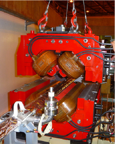
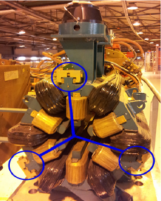
Refer to captionRefer to caption

Figure 13: (Color) Mechanical assemblies of the ESRF magnets: Quadrupoles are separated in two halves (left), whereas three yokes are screwed together to create sextupoles (right) with survey monuments being placed on one arc only.

The resulting rms sextupole rotation is of about 1.3 mrad, with some magnets exceeding ±3plus-or-minus3\pm 3 mrad. Again, results vary according to the number of eigen-values. However, metrological surveys ensure rms girder rotations well below 0.1 mrad and it is hard to believe that magnets installed onto them may account for more than 1 mrad. An alternative explanation for such large skew sextupole components has been proposed and is currently being investigated. During magnetic measurements of new quadrupole magnets a large skew quadrupole component was measured each time the two halves of the yoke were not properly aligned (see left picture of Fig. 13): For that specific magnet, as a rule of thumb, a horizontal displacement between the two yokes of 100 μ𝜇\mum would generated a skew quadrupole field, corresponding to about 1 mrad equivalent rotation. This sensitivity is suspected to be of importance for sextupoles too, these being actually separated in three yokes (right picture of Fig. 13). Numerical simulations and magnetic measurements are planned to validate this conjecture. If confirmed, hence, the large skew sextupole components observed in the ESRF storage ring may be induced by the limited precision in the assembly of the three sextupole yokes, rather than by the physical magnet rotation as a whole.

IV.4 Correction of sextupolar CRDTs
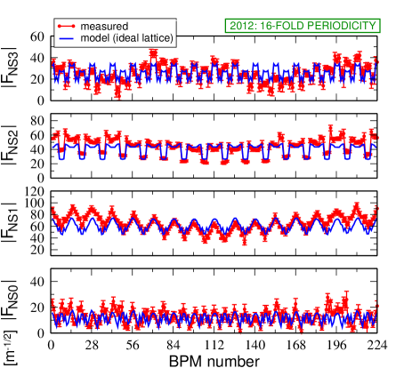
Refer to captionRefer to caption


Figure 14: (Color) Measured (red) and ideal (blue) normal sextupole CRDTs of the fully 16-fold periodic ESRF storage ring (left, 2012) and of the new configuration with a longer straight section which breaks up the symmetry (right, 2013). The position of this longer section (and of the corresponding insertion optics) is represented by the vertical green line. Even in absence of focusing errors the CRDTs (i.e. the blue curve of the right plot) are substantially modified by this insertion.

After building up a realistic sextupolar error model, the natural further step would be to use the measured CRDTs (\vvFNS,meas\vvsubscript𝐹𝑁𝑆𝑚𝑒𝑎𝑠\vv{F}_{NS,meas}) and the desired one (\vvFNS,ref\vvsubscript𝐹𝑁𝑆𝑟𝑒𝑓\vv{F}_{NS,ref}), insert them in the linear system of Eq. (12), and pseudo-invert it to evaluate the strengths of the available sextupole correctors. The desired CRDTs are those assuming an ideal lattice, with neither errors (linear and nonlinear) nor betatron coupling. If special insertions spoiling the machine periodicity are present, they may induce large CRDT modulations. This is the case of the ESRF as of 2013, when a straight section was lengthened from 5 to 7 m and a special insertion optics was implemented. The impact on the normal sextupole CRDTs is strong, as shown in Fig. 14. When correcting the CRDTs, the reference vector \vvFNS,ref\vvsubscript𝐹𝑁𝑆𝑟𝑒𝑓\vv{F}_{NS,ref} corresponding to the fully periodic machine (i.e. without the insertion) was chosen. The result of such an exercise is shown in Fig. 15, where the difference vector \vvFNS,meas\vvsubscript𝐹𝑁𝑆𝑚𝑒𝑎𝑠\vv{F}_{NS,meas}- \vvFNS,ref\vvsubscript𝐹𝑁𝑆𝑟𝑒𝑓\vv{F}_{NS,ref} is plotted before and after the correction, together with the corresponding strengths of the 19 available sextupole correctors.
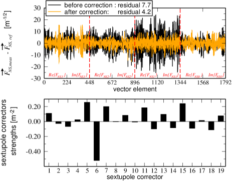
Refer to caption

Figure 15: (Color) Example of normal sextupole CRDT correction. Top: difference between the measured and the reference CRDT vectors before (black) and after (orange) correction. Bottom: integrated strengths of the corresponding 19 available sextupole correctors.

Even if elegant and efficient (the rms residual is almost halved with just 19 correctors out of 224 sources of errors), this approach is rather inconvenient. The reason is three-fold. First, the sextupole error model may depend on the implemented optics. The one used for these measurements has been specifically tuned so to have high spectral resolution but would be impractical for operational purposes. On the other hand, it would be impossible to extract an error model from the operational settings with the same accuracy, because of their larger chromaticity and detuning. Depending on the filling mode, chromatic sextupoles may vary considerably, and so may their errors, being the magnets close to saturation. Second, while focusing errors and coupling may be evaluated and corrected routinely from ORM measurements, the setup for the TbT BPM acquisition is less obvious and difficult to perform with the same regularity, even admitting that a sufficient spectral resolution may be found. Third, the special sextupole setting would not permit to verify whether the CRDT correction is beneficial to the beam lifetime, the chromaticity being too low for storing more than 10 mA, whereas 200 mA are usually delivered to users.

Table 7: Summary of the residual \mathcal{R} of Eq. (IV.3) between the measured normal sextupole CRDTs and different lattice models.
Model characteristics residual \mathcal{R}
[m-1/2]
ideal lattice + 2001 sextupole calibration 8.4
ideal lattice + 2012 sextupole calibration 7.7
lattice with focusing errors
     + 2012 sextupole calibration 3.2
lattice with focusing errors
     + 2012 sextupole calibration 1.8
     + sextupole errors

A rapid look at the evolution of the residual \mathcal{R} as a function of the lattice models may provide a handy, though not perfect, solution. Table 7 summarizes this dependence. Because of the relatively large persistent β𝛽\beta-beating in the ESRF storage ring, the main contribution to the the measured CRDTs (50%similar-toabsentpercent50\sim 50\%) originates from focusing errors, whereas only 25%percent2525\% seems to stem from sextupole errors and a further 25%percent2525\% is not accounted for (possibly because of higher-order terms affecting the sextupolar spectral lines, as shown in Fig. 7). This means that a detailed linear lattice model would describe the true CRDTs with an accuracy sufficient for their rough correction, even ignoring sextupole errors. This corresponds to use and correct the black (model) curves in the left plot of Fig. 9 instead of the (measured) red curves: Even if not perfect, the model CRDTs may already be used for an effective and rapid correction. This may be a peculiarity of machines like the one at the ESRF. For more recent accelerators with independent magnets, and hence with much lower residual focusing errors, this may not be the case.

To verify this conjecture, a test during machine-dedicated time was carried out. The software application for the measurement of the ORM and correction of focusing and coupling errors was modified to compute the normal sextupole CRDTs FNSsubscript𝐹𝑁𝑆F_{NS} from the lattice model ( i.e. from Tables 3 and 2), including all errors. These were inserted in the \vvFNS,meas\vvsubscript𝐹𝑁𝑆𝑚𝑒𝑎𝑠\vv{F}_{NS,meas} vector, whereas the ideal C-S parameters were used to compute the ideal (and desired) CRDTs,r \vvFNS,ref\vvsubscript𝐹𝑁𝑆𝑟𝑒𝑓\vv{F}_{NS,ref}. The system of Eq. (12) was then pseudo-inverted to infer the strengths of the sextupole correctors. This procedure was applied to a standard multibunch optics optimized for a train of 868 bunches (7/8 of the storage ring circumference) filled with 200 mA (i.e. 0.23 mA per bunch). To enhance the Touschek effect which is believed to be presently the main limitation for the lifetime, another filling pattern with 192 bunches, each of about 1 mA, was stored. With all sextupole correctors turned off and a vertical emittance ϵy=7.1subscriptitalic-ϵ𝑦7.1\epsilon_{y}=7.1 pm (ϵx=4subscriptitalic-ϵ𝑥4\epsilon_{x}=4 nm), a lifetime of 16.2 hours was measured. After applying the standard manual optimization of the four sextupolar resonance stopbands, the lifetime reached 24.2 hours. When the strength computed automatically from Eq. (12) were used, the measured lifetime was 22.4 hours. This proved the effectiveness of the method, which can be used for a first correction from scratch before trimming the correctors by hand with the standard ESRF procedure. Nevertheless, it turned out to be not yet optimal. Another test was carried out to a different optics with higher chromaticity (to stabilize higher charges per bunch) clearly showed a poorer performance of the CRDT correction compared to the standard procedure. The reason for this dependence on the implemented optics has not been yet understood.

IV.5 Beam-based calibration of independent sextupoles via CRDTs
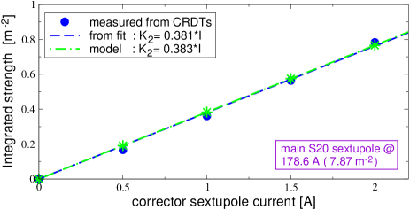
Refer to caption

Refer to caption

Refer to caption

Figure 16: (Color) Beam-based calibration of sextupole correctors (trim coils) from measurements of CRDTs and Eq. (11). For two correctors in cell 8 of the ESRF storage ring the curves have been measured in detail with several points: S20C8 is hosted in a chromatic sextupole (top plot) close to saturation, hence with a coefficient lower than in the correctors installed in the harmonic sextupoles, such as S24C8 (centre plot), which are still in the linear regime. The measured coefficients (i.e. the slopes of the above plots) for all twelve trim coils are reported in the bottom chart.

As discussed in the last paragraph of Sec. III.5, the measurement of CRDTs FNSsubscript𝐹𝑁𝑆F_{NS} may be repeated for different gradients of individual sextupoles or correctors to obtain a calibration curve, (integrated) strength Vs current. The ESRF storage ring comprises of 224 sextupoles mostly grouped in seven families, each sharing a common power supply. Six new short magnets recently installed to lengthen three straight sections are fed independently, and two standard sextupoles have been stripped out and paired on a single power supply. The correction of sextupolar resonances is carried out by twelve correctors (trim coils) hosted in as many magnets of the families 24 (eight) and \verb 20 (four). Even though magnetically identical, because of the different working points, the (stronger) chromatic

20  are close
to saturation, whereas the (weaker) harmonic \verb 
24 are still in the linear regime. This results in trim coils with different calibration curves, i.e. the slopes Cfsubscript𝐶𝑓C_{f} of the linear curve K2=CfIsubscript𝐾2subscript𝐶𝑓𝐼K_{2}=C_{f}\cdot I, where I𝐼I denotes the imparted current.

By measuring the CRDTs it is then possible to validate the calibration of both the trim coils and the six independent short sextupoles

4 .
The first check is necessary for the effectiveness of the
automatic resonance correction discussed in the previous
section, whereas the latter is to confirm the hypothesis
raised in 
ec. IV.3 of having short sextupoles weaker than expected.
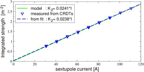
Refer to caption

Figure 17: (Color) Beam-based calibration of short independent sextupole S4C15 from measurements of CRDTs and Eq. (11).

For two trim coils in cell 8 (20C8 and \verb 24C8 ) the measurement has been carried out with several points and the calibration coefficient is obtained from a linear fit of the curve K2=CfIsubscript𝐾2subscript𝐶𝑓𝐼K_{2}=C_{f}\cdot I. As shown in the upper plots of Fig. 16 the agreement with the model is nearly perfect for the corrector 20C8 , and compatible within $10\%$ for \verb 24C8 . The same measurement was then repeated for the other ten correctors. Results are reported in the bottom chart of Fig. 16. Because of the limited available machine time, the linear fit for the remaining ten correctors was carried out with two points only, at ±1plus-or-minus1\pm 1 A. Between each measurement, magnets were not cycled and the persistence of some remaining magnetic fields could not be excluded. If these arguments may explain the poorer agreement between model and measured coefficients for these ten correctors, they cannot justify the large discrepancy observed for two trim coils, in 24C23 and \verb 24C29 respectively. As far as the corrector in cell 23 is concerned, the explanation is rather simple: As of 2013 the standard 40 cm long main magnet has been replaced by a new short type. As a result, the calibration for its corrector is almost halved (Cfsubscript𝐶𝑓C_{f} from 0.4430.4430.443 to 0.2390.2390.239 A-1m2), consistent with the measured value. In the case of the trim coils of

24C29 , an inconsistency was indeed found
between the power supplies (recent 2-A types) and one of
the two driver cards (still set for an old 5-A type).
This incongruity resulted in a corrector about $30\%$
weaker than normal ($C_f$ from $0.443$ to $0.310$~A$^{-1}$m$^2$),
again consistent with measurements. Following
these findings, the software driving the trim coil
\verb 
24C23 has been updated (it was not when testing the automatic resonance correction), and the driver card of
24C29  was updated.
Results from the same measurement carried out for one
of the six new (short and independent) sextupoles in cell
15, \verb 
4C15 , are reported in Fig. 17. This beam-based calibration (Cf=0.0238±0.002subscript𝐶𝑓plus-or-minus0.02380.002C_{f}=0.0238\pm 0.002 A-1m2) is compatible with magnetic measurement (Cf=0.0241subscript𝐶𝑓0.0241C_{f}=0.0241).

V Going beyond: octupolar spectral lines, CRDTs and modelling

Figure 7 reveals the existence of four spectral lines well above noise level (and hence measurable) excited by octupolar CRDTs, namely H(3,0)𝐻30H(3,0), H(1,2)𝐻12H(-1,2), V(2,1)𝑉21V(2,1) and V(2,1)𝑉21V(2,-1). As shown in the same figure and described in Table 9, two additional lines are excited by these terms, H(1,2)𝐻12H(1,2) and V(0,3)𝑉03V(0,3). However, the latter are indistinguishable from the sextupolar lines H(0,2)𝐻02H(0,-2) and V(1,1)𝑉11V(-1,-1), respectively, because of the tune working point. Hence the corresponding CRDTs FNO4subscript𝐹𝑁𝑂4F_{NO4} and FNO5subscript𝐹𝑁𝑂5F_{NO5} of Table 9 are not observable in our case. The best setting for the ESRF storage ring turned out to be the last of Table 4, with the horizontal kicker fired at 400 A and the vertical at 3.0 kV. The formulas of Table 9 to infer the octupolar CRTDs from the spectral lines have been corrected in the analysis by using the tune line amplitudes averaged among all 224 BPMs, i.e. |H(1,0)|<|H(1,0)|>𝐻10expectation𝐻10|H(1,0)|\rightarrow<|H(1,0)|> and |V(0,1)|<|V(0,1)|>𝑉01expectation𝑉01|V(0,1)|\rightarrow<|V(0,1)|> in order to reduce the impact of octupolar terms on the tune line (see discussion in the last part of Appendix D).
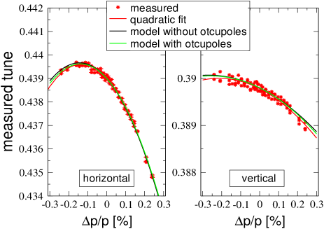
Refer to caption

Refer to caption

Figure 18: (Color) Nonlinear chromaticity (top two graphs) and linear amplitude dependent detuning (bottom three plots). The measured curves (red) are compared to the ones computed from lattice model including all errors up to the sextupolar components (black), and after including octupolar components in the main quadrupoles (green). The corresponding coefficients are listed in the Tk-FF columns (thick sextupoles and fringe fields in all magnets) of Table 10.

Even though no physical octupole is installed in the ESRF storage ring, the nonlinear model including sextupoles (with errors and tilts) alone does not suffice to reproduce global nonlinear parameters such as amplitude dependent detuning ν=Qsuperscript𝜈𝑄\nu^{\prime}=\partial Q/(2I)2𝐼\partial(2I), as reported in Table 10 and Fig. 18. The agreement between this model and measurements is however already good as far as the second-order chromatic terms Q′′=2Qsuperscript𝑄′′superscript2𝑄Q^{\prime\prime}=\partial^{2}Q/δ2superscript𝛿2\partial\delta^{2} are concerned. As stressed in Sec. III.1, no significant difference has been observed in the RDTs when representing sextupoles either as thin or thick elements and when including fringe fields. This is not the case for the global nonlinear parameters and in Table 10 values for the three different models are reported. Plots and fit (of global parameters and octupolar CRDTs) however refer to the thick model and including fringe fields.

Table 8: List of lines in the spectra of x~(N)~𝑥𝑁\tilde{x}(N) and y~(N)~𝑦𝑁\tilde{y}(N) excited by normal octupole CRDTs F=|F|eiqF𝐹𝐹superscript𝑒𝑖subscript𝑞𝐹F=|F|e^{iq_{F}} and excited resonances. For each line (defined as in Table 2), expressions for its amplitude and phase are given. The tune lines H(1,0)𝐻10H(1,0) and V(0,1)𝑉01V(0,1) are also affected by octupolar terms that are however not observable. Quadrupole errors are to be included in the model when computing the Courant-Snyder (C-S) parameters used to evaluate x~(N)~𝑥𝑁\tilde{x}(N), y~(N)~𝑦𝑁\tilde{y}(N) and the CRDTs gjklmsubscript𝑔𝑗𝑘𝑙𝑚g_{jklm}, which are defined in Table 15.
spectral line      amplitude phase ϕitalic-ϕ\phi Combined RDT    resonances magnetic term
V(0,3)𝑉03V(0,3) (2Iy)3/2|FNO5|superscript2subscript𝐼𝑦32subscript𝐹𝑁𝑂5(2I_{y})^{3/2}|F_{NO5}| qFNO3+π2+3ψy0subscript𝑞subscript𝐹𝑁𝑂3𝜋23subscript𝜓𝑦0q_{F_{NO3}}+\frac{\pi}{2}+3\psi_{y0} FNO5=4g0040g0013subscript𝐹𝑁𝑂54superscriptsubscript𝑔0040subscript𝑔0013F_{NO5}=4g_{0040}^{*}-g_{0013} (0,4),(0,2) y4superscript𝑦4y^{4}
H(1,2)𝐻12H(1,2) (2Ix)1/2(2Iy)|FNO4|superscript2subscript𝐼𝑥122subscript𝐼𝑦subscript𝐹𝑁𝑂4(2I_{x})^{1/2}(2I_{y})|F_{NO4}| qFNO4+π2+ψx0+2ψy0subscript𝑞subscript𝐹𝑁𝑂4𝜋2subscript𝜓𝑥02subscript𝜓𝑦0q_{F_{NO4}}+\frac{\pi}{2}+\psi_{x0}+2\psi_{y0} FNO4=2g2020,Hg1102subscript𝐹𝑁𝑂42superscriptsubscript𝑔2020𝐻subscript𝑔1102F_{NO4}=2g_{2020,H}^{*}-g_{1102} (2,2),(0,2) x2y2superscript𝑥2superscript𝑦2x^{2}y^{2}
H(3,0)𝐻30H(3,0) (2Ix)3/2|FNO3|superscript2subscript𝐼𝑥32subscript𝐹𝑁𝑂3(2I_{x})^{3/2}|F_{NO3}| qFNO3+π2+3ψx0subscript𝑞subscript𝐹𝑁𝑂3𝜋23subscript𝜓𝑥0q_{F_{NO3}}+\frac{\pi}{2}+3\psi_{x0} FNO3=4g4000g1300subscript𝐹𝑁𝑂34superscriptsubscript𝑔4000subscript𝑔1300F_{NO3}=4g_{4000}^{*}-g_{1300} (4,0),(2,0) x4superscript𝑥4x^{4}
H(1,2)𝐻12H(-1,2) (2Ix)1/2(2Iy)|FNO2|superscript2subscript𝐼𝑥122subscript𝐼𝑦subscript𝐹𝑁𝑂2(2I_{x})^{1/2}(2I_{y})|F_{NO2}| qFNO2π2ψx0+2ψy0subscript𝑞subscript𝐹𝑁𝑂2𝜋2subscript𝜓𝑥02subscript𝜓𝑦0q_{F_{NO2}}-\frac{\pi}{2}-\psi_{x0}+2\psi_{y0} FNO2=2g2002g1120subscript𝐹𝑁𝑂22subscript𝑔2002superscriptsubscript𝑔1120F_{NO2}=2g_{2002}-g_{1120}^{*} (2,-2),(0,2) x2y2superscript𝑥2superscript𝑦2x^{2}y^{2}
V(2,1)𝑉21V(2,-1) (2Ix)(2Iy)1/2|FNO1|2subscript𝐼𝑥superscript2subscript𝐼𝑦12subscript𝐹𝑁𝑂1(2I_{x})(2I_{y})^{1/2}|F_{NO1}| qFNO1π2+2ψx0ψy0subscript𝑞subscript𝐹𝑁𝑂1𝜋22subscript𝜓𝑥0subscript𝜓𝑦0q_{F_{NO1}}-\frac{\pi}{2}+2\psi_{x0}-\psi_{y0} FNO1=2g0220g2011subscript𝐹𝑁𝑂12subscript𝑔0220superscriptsubscript𝑔2011F_{NO1}=2g_{0220}-g_{2011}^{*} (2,-2),(2,0) x2y2superscript𝑥2superscript𝑦2x^{2}y^{2}
V(2,1)𝑉21V(2,1) (2Ix)(2Iy)1/2|FNO0|2subscript𝐼𝑥superscript2subscript𝐼𝑦12subscript𝐹𝑁𝑂0(2I_{x})(2I_{y})^{1/2}|F_{NO0}| qFNO0+π2+2ψx0+ψy0subscript𝑞subscript𝐹𝑁𝑂0𝜋22subscript𝜓𝑥0subscript𝜓𝑦0q_{F_{NO0}}+\frac{\pi}{2}+2\psi_{x0}+\psi_{y0} FNO0=2g2020,Vg0211subscript𝐹𝑁𝑂02superscriptsubscript𝑔2020𝑉subscript𝑔0211F_{NO0}=2g_{2020,V}^{*}-g_{0211} (2,2),(2,0) x2y2superscript𝑥2superscript𝑦2x^{2}y^{2}
Table 9: Formulas to evaluate octupolar CRDTs from the secondary lines in the spectra of x~(N)~𝑥𝑁\tilde{x}(N) and y~(N)~𝑦𝑁\tilde{y}(N) assuming properly calibrated BPMs, turn-by-turn oscillations without decoherence and quadrupole errors included in the C-S parameters.
Combined RDT                  amplitude          phase qFsubscript𝑞𝐹q_{F}
FNO5=|FNO5|eiqFNO5subscript𝐹𝑁𝑂5subscript𝐹𝑁𝑂5superscript𝑒𝑖subscript𝑞subscript𝐹𝑁𝑂5F_{NO5}=|F_{NO5}|e^{iq_{F_{NO5}}} |FNO5|=|V(0,3)|/[8|V(0,1)|3]subscript𝐹𝑁𝑂5𝑉03delimited-[]8superscript𝑉013|F_{NO5}|=|V(0,3)|/[8|V(0,1)|^{3}] qFNO5=ϕV(0,3)3ϕV(0,1)π2subscript𝑞subscript𝐹𝑁𝑂5subscriptitalic-ϕ𝑉033subscriptitalic-ϕ𝑉01𝜋2q_{F_{NO5}}=\phi_{V(0,3)}-3\phi_{V(0,1)}-\frac{\pi}{2}
FNO4=|FNO4|eiqFNO4subscript𝐹𝑁𝑂4subscript𝐹𝑁𝑂4superscript𝑒𝑖subscript𝑞subscript𝐹𝑁𝑂4F_{NO4}=|F_{NO4}|e^{iq_{F_{NO4}}} |FNO4|=|H(1,2)|/[8|H(1,0)||V(0,1)|2]subscript𝐹𝑁𝑂4𝐻12delimited-[]8𝐻10superscript𝑉012|F_{NO4}|=|H(1,2)|/[8|H(1,0)||V(0,1)|^{2}] qFNO4=ϕH(1,2)ϕH(1,0)2ϕV(0,1)π2subscript𝑞subscript𝐹𝑁𝑂4subscriptitalic-ϕ𝐻12subscriptitalic-ϕ𝐻102subscriptitalic-ϕ𝑉01𝜋2q_{F_{NO4}}=\phi_{H(1,2)}-\phi_{H(1,0)}-2\phi_{V(0,1)}-\frac{\pi}{2}
FNO3=|FNO3|eiqFNO3subscript𝐹𝑁𝑂3subscript𝐹𝑁𝑂3superscript𝑒𝑖subscript𝑞subscript𝐹𝑁𝑂3F_{NO3}=|F_{NO3}|e^{iq_{F_{NO3}}} |FNO3|=|H(3,0)|/[8|H(1,0)|3]subscript𝐹𝑁𝑂3𝐻30delimited-[]8superscript𝐻103|F_{NO3}|=|H(3,0)|/[8|H(1,0)|^{3}] qFNO3=ϕH(3,0)3ϕH(1,0)π2subscript𝑞subscript𝐹𝑁𝑂3subscriptitalic-ϕ𝐻303subscriptitalic-ϕ𝐻10𝜋2q_{F_{NO3}}=\phi_{H(3,0)}-3\phi_{H(1,0)}-\frac{\pi}{2}
FNO2=|FNO2|eiqFNO2subscript𝐹𝑁𝑂2subscript𝐹𝑁𝑂2superscript𝑒𝑖subscript𝑞subscript𝐹𝑁𝑂2F_{NO2}=|F_{NO2}|e^{iq_{F_{NO2}}} |FNO2|=|H(1,2)|/[8|H(1,0)||V(0,1)|2]subscript𝐹𝑁𝑂2𝐻12delimited-[]8𝐻10superscript𝑉012|F_{NO2}|=|H(-1,2)|/[8|H(1,0)||V(0,1)|^{2}] qFNO2=ϕH1,2)+ϕH(1,0)2ϕV(0,1)+π2q_{F_{NO2}}=\phi_{H-1,2)}+\phi_{H(1,0)}-2\phi_{V(0,1)}+\frac{\pi}{2}
FNO1=|FNO1|eiqFNO1subscript𝐹𝑁𝑂1subscript𝐹𝑁𝑂1superscript𝑒𝑖subscript𝑞subscript𝐹𝑁𝑂1F_{NO1}=|F_{NO1}|e^{iq_{F_{NO1}}} |FNO1|=|V(2,1)|/[8|H(1,0)|2|V(0,1)|]subscript𝐹𝑁𝑂1𝑉21delimited-[]8superscript𝐻102𝑉01|F_{NO1}|=|V(2,-1)|/[8|H(1,0)|^{2}|V(0,1)|] qFNO1=ϕV(2,1)2ϕH(1,0)+ϕV(0,1)+π2subscript𝑞subscript𝐹𝑁𝑂1subscriptitalic-ϕ𝑉212subscriptitalic-ϕ𝐻10subscriptitalic-ϕ𝑉01𝜋2q_{F_{NO1}}=\phi_{V(2,-1)}-2\phi_{H(1,0)}+\phi_{V(0,1)}+\frac{\pi}{2}
FNO0=|FNO0|eiqFNO0subscript𝐹𝑁𝑂0subscript𝐹𝑁𝑂0superscript𝑒𝑖subscript𝑞subscript𝐹𝑁𝑂0F_{NO0}=|F_{NO0}|e^{iq_{F_{NO0}}} |FNO0|=|V(2,1)|/[8|H(1,0)|2|V(0,1)|]subscript𝐹𝑁𝑂0𝑉21delimited-[]8superscript𝐻102𝑉01|F_{NO0}|=|V(2,1)|/[8|H(1,0)|^{2}|V(0,1)|] qFNO0=ϕV(2,1)2ϕH(1,0)ϕV(0,1)π2subscript𝑞subscript𝐹𝑁𝑂0subscriptitalic-ϕ𝑉212subscriptitalic-ϕ𝐻10subscriptitalic-ϕ𝑉01𝜋2q_{F_{NO0}}=\phi_{V(2,1)}-2\phi_{H(1,0)}-\phi_{V(0,1)}-\frac{\pi}{2}

Refer to caption       Refer to caption

Figure 19: (Color) Amplitudes of normal octupole CRDTs (red curves) measured at the ESRF storage ring (with a special dedicated optics). Left: comparison with the model curves obtained from a lattice with no octupolar source (CRDTs are excited by sextupoles to the second order only). Right: comparison with the same model after introducing octupole components in quadrupoles so to fit the nonlinear parameters of Table 10 and the measured octupolar CRDTs.

Table 10: Detuning coefficients and second-order chromaticity for the special lattice optics studied throughout this paper. Measured values are listed in the first column, whereas the corresponding numbers for the lattice model (all comprising the errors inferred in the previous sections) are reported in the second column. The model is presented in three flavors: thin (Tn) and thick (Tk) sextupoles, and with additional fringe fields in all magnets (Tk-FF). Octupolar fields are introduced in the 256 main normal quadrupoles to reproduce the measured coefficients (first) and the octupolar CRTDs (then), yielding to the values in the last column.
model model
parameter   measured without with
octupoles octupoles
Tk-FF      Tk        Tn Tk-FF
νxxsuperscriptsubscript𝜈𝑥𝑥\nu_{xx}^{\prime}  [m-1] 2430±plus-or-minus\pm30 -1396    (-2515)    (4185) 2364
νxysuperscriptsubscript𝜈𝑥𝑦\nu_{xy}^{\prime}  [m-1] -470±plus-or-minus\pm15 1289     ( -115)    (4962) -521
νyysuperscriptsubscript𝜈𝑦𝑦\nu_{yy}^{\prime}  [m-1] 4750±plus-or-minus\pm50 3485    ( 2518)    (8206) 4846
Qx′′superscriptsubscript𝑄𝑥′′Q_{x}^{\prime\prime}\hskip 20.48596pt[ ] 683±24plus-or-minus68324-683\pm 24 -649    (-657)     (-522) -660
Qy′′superscriptsubscript𝑄𝑦′′Q_{y}^{\prime\prime}\hskip 20.48596pt[ ] 96±17plus-or-minus9617-96\pm 17 -67     ( -74)     ( -30) -82

To the first order, sextupoles do not drive any detuning with amplitude, which is a second-order effect (i.e. induced by cross-product between sextupole terms). Octupolar CRDTs too are excited by second-order sextupolar terms even in absence of physical octupoles. This can be seen when comparing the four measured octupolar CRDTs with those evaluated from the lattice model (including all errors), as shown in the left plot of Fig. 19. Even though the global behavior is rather well reproduced by the model, a clear ingredient looks missing. Model CRDTs are evaluated by using the same procedure developed for the skew sextupole terms and described in Appendix A.

The first natural source of octupolar fields in a storage ring is represented by normal quadrupoles, because of the shape of their poles, fringe fields and their geometry in two halves (any variation of the vertical distance between the two yokes generates octupolar fields). The linear lattice of the ESRF storage ring is based on eight quadrupoles per cell (256 magnets in total), with two pairs of identical magnets in the achromat fed by common power supplies, hence leaving six degrees of freedom. The first step in building the octupolar lattice model was to introduce six octupolar fields in the corresponding quadrupole families to best reproduce the five nonlinear parameters (three detuning coefficients and two second-order chromatic terms). The 256 octupole fields have been then adjusted independently so to best reproduce the measured CRDTs of Fig. 19. As for the skew sextupole analysis, even though model and measured CRDTs are excited mainly by second-order contributions stemming from sextupoles, their difference will

depend linearly on the octupolar field, and the same SVD pseudo-inversion carried out in the previous sections may be generalized to octupoles. The results of such a fit are shown in the right plot of Fig. 19 as far as the CRDTs are concerned, whereas the values of the global nonlinear parameters are reported in the last column of Table 10 and in Fig. 18.

It shall be mentioned that measurements of octupolar CRDTs may be partially affected by BPM nonlinearities, these scaling with x3superscript𝑥3x^{3} (y3superscript𝑦3y^{3}) to the first order soleil and the largest BPM data used for this analysis reaching about 6 mm. On the other hand, the software driving the ESRF BPMs computes the beam position using a nonlinear calibration curve, based on finite-element simulations of the BPM block, that accounts already for such nonlinearities.

VI Conclusion

This paper has shown how the harmonic analysis of turn-by-turn data from beam position monitors may be exploited for the reconstruction and correction of machine nonlinearities up to octupolar terms. An important peculiarity of this approach is that the systems to be solved are always linear, even though referring to nonlinear magnets. This represents a considerable step forward compared to precedent works on the same subject. Handy formulas have been derived and tested with real data for the quantitative evaluation of realistic magnetic model, for the calibration of individual nonlinear magnets and for the correction of the resonance driving terms. The analysis of the latter could predict the sextupolar field component measured in bending magnets, as well some inconsistencies with the calibration curves of sextupole magnets. Correcting sextupolar resonance driving terms in the ESRF storage ring with a low-chromaticity optics (for low-intensity multi-bunch modes) resulted in increased lifetime, though the gain was minimal when applied to optics with larger chromaticity (for high-intensity few-bunch filling patterns).

VII Acknowledgments

We are grateful to the ESRF Operation Group for its support in preparing and carrying out measurements, to F. Epaud for adjusting the BPM device server to our needs, to M. Dubrulle for setting up the kickers, and to F. Taoutaou for helping with the magnetic measurements. We are also indebted with R. Tomás, for proofreading the original manuscript and making valuable suggestions.

Appendix A Nonresonant normal forms and RDTs up to the 2nd order

For a reliable analysis of the ESRF nonlinear lattice model, the normal form and RDT description of Refs. Bartolini1 ; Rogelio1 ; Andrea-thesis ; prstab_strength needs to be extended to the second order. The theoretical background has been already developed in previous works, among which the fundamental Ref. Bengtsson . The first part of this Appendix does not provide any further development to that work: Results of main interest in the context of this article are reported for sake of consistency and nomenclature only. In order to tackle the heavy mathematics of second-order computations, it may be desirable to briefly review the concept of nonresonant normal forms of Refs. Turchetti1 ; Forest1 .
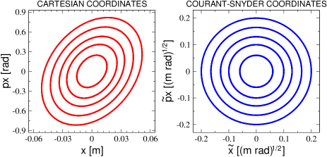
Refer to caption

Figure 20: Horizontal phase space portrait corresponding to the linear, uncoupled, betatron motion induced by normal quadrupoles in Cartesian coordinates (left) and in Courant-Snyder’s (right).

In the linear uncoupled case the turn-by-turn dynamics is described by the one-turn matrix M(s)𝑀𝑠M(s) according to

xs+C=M(s)xs,subscript𝑥𝑠𝐶𝑀𝑠subscript𝑥𝑠\vec{x}_{s+C}=M(s)\vec{x}_{s}\ , (21)

where C𝐶C is the ring circumference and s𝑠s a generic position along the ring. The corresponding phase space portrait (x,px𝑥subscript𝑝𝑥x,\ p_{x}) of the betatronic motion inside a circular accelerator is typically a tilted ellipse (identical considerations apply of course to the vertical plane). Tilt and main axis vary along the ring according to the focusing lattice (normal quadrupoles). Any regular (i.e. noncahotic) closed curve in phase-space may be transformed into a circle. The Courant-Snyder change of coordinates (Fig. 20)

(x~p~x)=((βx)1/20αx(βx)1/2(βx)1/2)(xpx)~𝑥missing-subexpressionsubscript~𝑝𝑥superscriptsubscript𝛽𝑥120missing-subexpressionmissing-subexpressionsubscript𝛼𝑥superscriptsubscript𝛽𝑥12superscriptsubscript𝛽𝑥12𝑥missing-subexpressionsubscript𝑝𝑥\left(\begin{array}[]{c}\tilde{x}\\ \\ \tilde{p}_{x}\end{array}\right)=\left(\begin{array}[]{c c}(\beta_{x})^{-1/2}&0\\ \\ \alpha_{x}(\beta_{x})^{-1/2}&(\beta_{x})^{1/2}\end{array}\right)\left(\begin{array}[]{c}x\\ \\ p_{x}\end{array}\right)

is one among the possible transformations preserving the phase-space. The Courant-Snyder (C-S) parameters in the above matrix contain all the information regarding the linear lattice. The circle is invariant along the ring in amplitude (i.e. radius and surface) and rotation frequency (i.e. the tune), which is independent on the initial conditions. The system is equivalent to a harmonic oscillator and the motion to a rotation.

In the nonlinear case the one-turn map (s)𝑠\mathcal{M}(s) replaces the linear matrix M(s)𝑀𝑠M(s)

xs+C=(s)xs,subscript𝑥𝑠𝐶𝑠subscript𝑥𝑠\vec{x}_{s+C}=\mathcal{M}(s)\vec{x}_{s}\ , (22)

where the map is the composition of linear transfer matrices Mwsubscript𝑀𝑤M_{w} and Lie operators corresponding to localized nonlinear magnets, such as sextupoles, see Fig. 21:

=MW+1w=1We:Hw:Mw,subscript𝑀𝑊1superscriptsubscriptproduct𝑤1𝑊superscript𝑒:absentsubscript𝐻𝑤:subscript𝑀𝑤\mathcal{M}=M_{W+1}\prod_{w=1}^{W}{e^{:H_{w}:}M_{w}}, (23)

where W𝑊W is the total number of nonlinear elements in the machine.
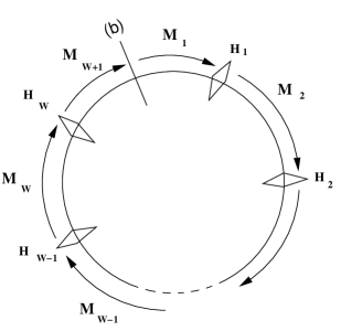
Refer to caption

Figure 21: Schematic view of a ring and its transfer maps, Mwsubscript𝑀𝑤M_{w} refer to sections free of nonlinearities, Hwsubscript𝐻𝑤H_{w} represent the nonlinear kicks.

Besides Ref. Bengtsson , detailed derivation within the RDT formalism may be found in Refs. Bartolini1 ; Rogelio1 ; Andrea-thesis . In the complex Courant-Snyder coordinates, hq,±=q~±ip~q=2Jqei(ϕq+ϕq,0)subscript𝑞plus-or-minusplus-or-minus~𝑞𝑖subscript~𝑝𝑞2subscript𝐽𝑞superscript𝑒minus-or-plus𝑖subscriptitalic-ϕ𝑞subscriptitalic-ϕ𝑞0h_{q,\pm}=\tilde{q}\pm i\tilde{p}_{q}=\sqrt{2J_{q}}e^{\mp i(\phi_{q}+\phi_{q,0})}, the system reduces to

hs+C=~(s)hs,~=w=1We:H~w(s):R,formulae-sequencesubscript𝑠𝐶~𝑠subscript𝑠~superscriptsubscriptproduct𝑤1𝑊superscript𝑒:absentsubscript~𝐻𝑤𝑠:𝑅\vec{h}_{s+C}=\tilde{\mathcal{M}}(s)\vec{h}_{s}\ ,\qquad\tilde{\mathcal{M}}=\prod_{w=1}^{W}{e^{:\tilde{H}_{w}(s):}}R\ \ , (24)

where h=(hx,+,hx,,hy,+,hy,)subscript𝑥subscript𝑥subscript𝑦subscript𝑦\vec{h}=(h_{x,+},h_{x,-},h_{y,+},h_{y,-}), R𝑅R denotes the phase-space rotation, whose s frequencies are the betatron tunes. The one-turn Lie operator then reads

e:H~:=w=1We:H~w:,~(s)=e:H~:R,e^{:\tilde{H}:}=\prod_{w=1}^{W}{e^{:\tilde{H}_{w}:}}\quad,\quad\tilde{\mathcal{M}}(s)=e^{:\tilde{H}:}R\ \ , (25)

and the Hamiltonian term of the generic nonlinear magnet w𝑤w reads

H~w(s)subscript~𝐻𝑤𝑠\displaystyle\tilde{H}_{w}(s) =\displaystyle= n2jklmn=j+k+l+mhw,jklmei[(jk)Δϕw,x(s)+(lm)Δϕw,y(s)]×\displaystyle\sum_{n\geq 2}\hskip-5.69046pt\sum_{jklm}^{\ \ n=j+k+l+m}\hskip-11.38092pt{h_{w,jklm}e^{i[(j-k)\Delta\phi_{w,x}^{(s)}+(l-m)\Delta\phi_{w,y}^{(s)}]}}\times (26)
hw,x,+jhw,x,khw,y,+lhw,y,m,superscriptsubscript𝑤𝑥𝑗superscriptsubscript𝑤𝑥𝑘superscriptsubscript𝑤𝑦𝑙superscriptsubscript𝑤𝑦𝑚\displaystyle h_{w,x,+}^{j}h_{w,x,-}^{k}h_{w,y,+}^{l}h_{w,y,-}^{m}\ \ ,

where hw,q,±subscript𝑤𝑞plus-or-minush_{w,q,\pm} is the coordinate at the generic magnet w𝑤w, while Δϕw,q(s)Δsuperscriptsubscriptitalic-ϕ𝑤𝑞𝑠\Delta\phi_{w,q}^{(s)} is the phase advance between the latter and the observation point s𝑠s. n𝑛n denotes the magnet order: n=2,3,4𝑛234n=2,3,4 for quadrupoles, sextupoles and octupoles, respectively. The coefficients within the sums read

hw,jklmsubscript𝑤𝑗𝑘𝑙𝑚\displaystyle h_{w,jklm} =\displaystyle= [Kw,n1Ω(l+m)+iJw,n1Ω(l+m+1)]j!k!l!m!2j+k+l+mdelimited-[]subscript𝐾𝑤𝑛1Ω𝑙𝑚𝑖subscript𝐽𝑤𝑛1Ω𝑙𝑚1𝑗𝑘𝑙𝑚superscript2𝑗𝑘𝑙𝑚\displaystyle-\displaystyle\frac{\bigl{[}K_{w,n-1}\Omega(l+m)+iJ_{w,n-1}\Omega(l+m+1)\bigr{]}}{j!\quad k!\quad l!\quad m!\quad 2^{j+k+l+m}}
×il+m(βw,x)j+k2(βw,y)l+m2,superscript𝑖𝑙𝑚superscriptsubscript𝛽𝑤𝑥𝑗𝑘2superscriptsubscript𝛽𝑤𝑦𝑙𝑚2\displaystyle\times\ \ i^{l+m}\bigl{(}\beta_{w,x}\bigr{)}^{\frac{j+k}{2}}\bigl{(}\beta_{w,y}\bigr{)}^{\frac{l+m}{2}},
ΩΩ\displaystyle\Omega (i)𝑖\displaystyle(i) =1 if i is even,Ω(i)=0 if i is odd.formulae-sequenceabsent1 if 𝑖 is evenΩ𝑖0 if 𝑖 is odd\displaystyle=1\hbox{ if }i\hbox{ is even},\quad\Omega(i)=0\hbox{ if }i\hbox{ is odd}\qquad\ . (27)

Ω(i)Ω𝑖\Omega(i) is introduced to select either the normal or the skew multipoles. Kw,n1subscript𝐾𝑤𝑛1K_{w,n-1} and Jw,n1subscript𝐽𝑤𝑛1J_{w,n-1} are the integrated magnet strengths of the multipole expansion (MADX definition)

[n2(Kw,n1+iJw,n1)(xw+iyw)nn!]subscript𝑛2subscript𝐾𝑤𝑛1𝑖subscript𝐽𝑤𝑛1superscriptsubscript𝑥𝑤𝑖subscript𝑦𝑤𝑛𝑛-\Re\left[\sum_{n\geq 2}{(K_{w,n-1}+iJ_{w,n-1})\frac{(x_{w}+iy_{w})^{n}}{n!}}\right] (28)

from which Eqs. (26) and  (A) are derived when moving from the Cartesian coordinates to the complex Courant-Snyder’s: xw=βw,x(hw,x,+hw,x,+)/2subscript𝑥𝑤subscript𝛽𝑤𝑥subscript𝑤𝑥subscript𝑤𝑥2x_{w}=\sqrt{\beta_{w,x}}(h_{w,x,-}+h_{w,x,+})/2 and yw=βw,y(hw,y,+hw,y,+)/2subscript𝑦𝑤subscript𝛽𝑤𝑦subscript𝑤𝑦subscript𝑤𝑦2y_{w}=\sqrt{\beta_{w,y}}(h_{w,y,-}+h_{w,y,+})/2.

Refer to caption

Refer to caption

Figure 22: Horizontal phase space portrait corresponding to the linear betatron motion with normal sextupoles in Cartesian coordinates (left), in Courant-Snyder’s (upper right) and normal forms (lower right).

If nonlinear terms are of relevance, at sufficiently large amplitudes the phase space is deformed from ellipses to more complex curves. In the case of normal sextupoles, the horizontal phase space (x,px𝑥subscript𝑝𝑥x,\ p_{x}) assumes a typical triangular shape, as a result of additional harmonics excited by these magnets (see Table 2). The Courant-Snyder transformation, being linear, will just remove the dependence on the linear parameters, rotating the triangle in an upright position and smoothing out its distortion. However, the invariant circle may not retrieved, since the linear transformation may not include nonlinearities, see upper right portrait of Fig. 22. The phase-space trajectory being still closed and regular, it must still exist a transformation to retrieve a circle. Such transformation indeed exists and is a polynomial function F𝐹F

F=n2jklmn=j+k+l+mfjklmζx,+jζx,kζy,+lζy,m,𝐹subscript𝑛2superscriptsubscript𝑗𝑘𝑙𝑚𝑛𝑗𝑘𝑙𝑚subscript𝑓𝑗𝑘𝑙𝑚superscriptsubscript𝜁𝑥𝑗superscriptsubscript𝜁𝑥𝑘superscriptsubscript𝜁𝑦𝑙superscriptsubscript𝜁𝑦𝑚\displaystyle F=\sum_{n\geq 2}\sum_{jklm}^{n=j+k+l+m}{f_{jklm}\zeta_{x,+}^{j}\zeta_{x,-}^{k}\zeta_{y,+}^{l}\zeta_{y,-}^{m}}\ , (29)

where n𝑛n denotes the multipole order, fjklmsubscript𝑓𝑗𝑘𝑙𝑚f_{jklm} are the RDTs and ζq,±=2Iqei(ψq+ψq,0)subscript𝜁𝑞plus-or-minus2subscript𝐼𝑞superscript𝑒minus-or-plus𝑖subscript𝜓𝑞subscript𝜓𝑞0\zeta_{q,\pm}=\sqrt{2I_{q}}e^{\mp i(\psi_{q}+\psi_{q,0})} are the new complex normal form coordinates, which are the nonlinear generalization of the complex Courant-Snyder complex variable of hq,±subscript𝑞plus-or-minush_{q,\pm}. The normal form approach for the turn-by-turn betatron motion is usually depicted in the scheme of Ref. Turchetti1 :

   ~=e:H~:R~superscript𝑒:absent~𝐻:𝑅\tilde{\mathcal{M}}=e^{:\tilde{H}:}R
h(N)𝑁\vec{h}(N) absent\xrightarrow[]{\hskip 28.45274pt\ \hskip 28.45274pt} h(N+1)𝑁1\vec{h}(N+1)
F1superscript𝐹1absentF^{-1}\Bigg{\downarrow} F𝐹\Bigg{\uparrow}\quad F
ζ(N)𝜁𝑁\vec{\zeta}(N) absent\xrightarrow[]{\hskip 28.45274pt\ \hskip 28.45274pt} ζ(N+1)𝜁𝑁1\vec{\zeta}(N+1)
   𝖱=e:𝖧:R𝖱superscript𝑒:absent𝖧:𝑅\mathsf{R}=e^{:\mathsf{H}:}R

R𝑅R is the same rotation of Eq. (24), H~=H~(Jx,Jy,ϕx,ϕy)~𝐻~𝐻subscript𝐽𝑥subscript𝐽𝑦subscriptitalic-ϕ𝑥subscriptitalic-ϕ𝑦\tilde{H}=\tilde{H}(J_{x},J_{y},\phi_{x},\phi_{y}) is the phase-dependent Hamiltonian of Eq. (25) (J𝐽J and ϕitalic-ϕ\phi are the linear invariant and betatron phase), whereas 𝖧(Ix,Iy)𝖧subscript𝐼𝑥subscript𝐼𝑦\mathsf{H}(I_{x},I_{y}) is the phase-independent Hamiltonian in normal forms, with I𝐼I the nonlinear invariant. Any dependence on the angles would indeed be related to the existence of fixed points different from the origin, around which stable orbits may exist, hence creating discontinuous phase space trajectories, as the ones of Ref. MTE : In this (resonant) case, no regular transformation may convert all separated trajectories in continuous circles.

There are two ways to predict the evolution of the betatron coordinate h=(hx,+,hx,,hy,+,hy,)subscript𝑥subscript𝑥subscript𝑦subscript𝑦\vec{h}=(h_{x,+},h_{x,-},h_{y,+},h_{y,-}) after one turn: Either solving the problem in the Courant-Snyder coordinates h(N+1)=e:H~:Rh(N)𝑁1superscript𝑒:absent~𝐻:𝑅𝑁\vec{h}(N+1)=e^{:\tilde{H}:}R\ \vec{h}(N), or finding the generating function F𝐹F, moving into normal forms ζ(N)𝜁𝑁\vec{\zeta}(N), applying the amplitude-dependent rotation 𝖱𝖱\mathsf{R} and coming back to the Courant-Snyder coordinates h(N+1)=e:F:ζ(N+1)𝑁1superscript𝑒:absent𝐹:𝜁𝑁1\vec{h}(N+1)=e^{:F:}\vec{\zeta}(N+1). The second strategy, even if longer, turns out to be indeed the most effective. In fact, analytical expressions for the RDTs fjklmsubscript𝑓𝑗𝑘𝑙𝑚f_{jklm} (and hence for F𝐹F) may be derived up to a certain degree of precision (second order in this paper), while the evolution in normal form is already known, being an amplitude-dependent rotation, whose operator 𝖱𝖱\mathsf{R} is defined by the tunes (Qx,ysubscript𝑄𝑥𝑦Q_{x,y}) and the invariants (2Ix,y2subscript𝐼𝑥𝑦2I_{x,y}) only, all measurable quantities, as shown later. In normal forms, the circle surface π|ζ|2𝜋superscript𝜁2\pi|\zeta|^{2} is the new (nonlinear) invariant, see lower right portrait of Fig. 22. The nonlinearity is also transferred in the frequency, which exhibits a dependence on the amplitude |ζ|=2I𝜁2𝐼|\zeta|=\sqrt{2I} (amplitude-dependent tune). The system in these coordinates is equivalent to an anharmonic oscillator and the motion is a rotation whose frequency depends on the initial conditions. As the Courant-Snyder matrix contains all the information regarding the linear lattice, the RDTs of F𝐹F carry its nonlinear content.

The equation establishing the change of coordinates in normal form of the above scheme may be written in terms of the Lie operators

ζ(N+1)𝜁𝑁1\displaystyle\underbrace{\vec{\zeta}(N+1)} =\displaystyle= e:F:h(N+1)superscript𝑒:absent𝐹:𝑁1\displaystyle e^{:-F:}\underbrace{\vec{h}(N+1)}
(e:𝖧:Rζ(N))superscript𝑒:absent𝖧:𝑅𝜁𝑁\displaystyle\left(e^{:\mathsf{H}:}R\vec{\zeta}(N)\right) =\displaystyle= e:F:(e:H~:Rh(N))superscript𝑒:absent𝐹:superscript𝑒:absent~𝐻:𝑅𝑁\displaystyle e^{:-F:}\left(e^{:\tilde{H}:}R\underbrace{\vec{h}(N)}\right)
e:𝖧:Rζ(N)superscript𝑒:absent𝖧:𝑅𝜁𝑁\displaystyle e^{:\mathsf{H}:}R\vec{\zeta}(N) =\displaystyle= e:F:e:H~:R(e:F:ζ(N))superscript𝑒:absent𝐹:superscript𝑒:absent~𝐻:𝑅superscript𝑒:absent𝐹:𝜁𝑁\displaystyle e^{:-F:}e^{:\tilde{H}:}R\left(e^{:F:}\vec{\zeta}(N)\right)
[e:𝖧:R]ζ(N)delimited-[]superscript𝑒:absent𝖧:𝑅𝜁𝑁\displaystyle\left[e^{:\mathsf{H}:}R\right]\vec{\zeta}(N) =\displaystyle= [e:F:e:H~:Re:F:]ζ(N).delimited-[]superscript𝑒:absent𝐹:superscript𝑒:absent~𝐻:𝑅superscript𝑒:absent𝐹:𝜁𝑁\displaystyle\left[e^{:-F:}e^{:\tilde{H}:}Re^{:F:}\right]\vec{\zeta}(N)\ .

The above relation holding for any ζ(N)𝜁𝑁\vec{\zeta}(N), the following homological equation is obtained

e:𝖧:Rsuperscript𝑒:absent𝖧:𝑅\displaystyle e^{:\mathsf{H}:}R =\displaystyle= e:F:e:H~:Re:F:superscript𝑒:absent𝐹:superscript𝑒:absent~𝐻:𝑅superscript𝑒:absent𝐹:\displaystyle e^{:-F:}e^{:\tilde{H}:}Re^{:F:} (30)

Following the same procedure of Ref. Bengtsson , all operators may be decomposed in first- and second-order terms as follows

F𝐹\displaystyle F =\displaystyle= F(1)+F(2)superscript𝐹1superscript𝐹2\displaystyle F^{(1)}+F^{(2)} (31)
𝖧𝖧\displaystyle\mathsf{H} =\displaystyle= 𝖧(1)+𝖧(2)superscript𝖧1superscript𝖧2\displaystyle\mathsf{H}^{(1)}+\mathsf{H}^{(2)} (32)
H~~𝐻\displaystyle\tilde{H} =\displaystyle= H~(1)+H~(2)=w=1WH~w+12w=1Wu=1w1[H~u,H~w]superscript~𝐻1superscript~𝐻2superscriptsubscript𝑤1𝑊subscript~𝐻𝑤12superscriptsubscript𝑤1𝑊superscriptsubscript𝑢1𝑤1subscript~𝐻𝑢subscript~𝐻𝑤\displaystyle\tilde{H}^{(1)}+\tilde{H}^{(2)}=\sum\limits_{w=1}^{W}{\tilde{H}_{w}}+\frac{1}{2}\sum\limits_{w=1}^{W}{\sum\limits_{u=1}^{w-1}{\left[\tilde{H}_{u},\tilde{H}_{w}\right]}}

Equation (LABEL:eq:deco2) results from Eq. (25): The composition of Lie Operators indeed obeys to the Campbell-Backer-Hausdorff (CBH) theorem

e:A:e:B:e:C:=e:A+B+C+12{[A,B]+[A,C]+[B,C]}:+O(3rd),superscript𝑒:absent𝐴:superscript𝑒:absent𝐵:superscript𝑒:absent𝐶:superscript𝑒:absent𝐴𝐵𝐶12𝐴𝐵𝐴𝐶𝐵𝐶:𝑂superscript3rd\displaystyle e^{:A:}e^{:B:}e^{:C:}=e^{:A+B+C+\frac{1}{2}\left\{[A,B]+[A,C]+[B,C]\right\}:}+O(3^{{\tiny\hbox{rd}}})\ ,

where [,][,] denotes the Poisson bracket, the first term (A+B+C) is the first-order truncation while the rest is the second-order contribution. Higher-order terms are here included in the remainder O(3rd)𝑂superscript3rdO(3^{{\tiny\hbox{rd}}}). Being these operators polynomial functions, Eq. (30) apply to all coefficients hjklmsubscript𝑗𝑘𝑙𝑚h_{jklm} (for H~~𝐻\tilde{H}), fjklmsubscript𝑓𝑗𝑘𝑙𝑚f_{jklm} (for F𝐹F), 𝗁jjllsubscript𝗁𝑗𝑗𝑙𝑙\mathsf{h}_{jjll} (for 𝖧𝖧\mathsf{H}). The rotation R𝑅R then will also act to each term (ζx,+jζx,kζy,+lζy,m)superscriptsubscript𝜁𝑥𝑗superscriptsubscript𝜁𝑥𝑘superscriptsubscript𝜁𝑦𝑙superscriptsubscript𝜁𝑦𝑚(\zeta_{x,+}^{j}\zeta_{x,-}^{k}\zeta_{y,+}^{l}\zeta_{y,-}^{m}), i.e.

R=e2πi[(jk)Qx+(lm)Qy)],j,k,l,m.\displaystyle R=e^{2\pi i\left[(j-k)Q_{x}+(l-m)Q_{y})\right]}\ ,\qquad\forall\quad j,k,l,m\ .\qquad (35)

Since the Hamiltonian in normal forms must be phase independent (only 𝗁jjllsubscript𝗁𝑗𝑗𝑙𝑙\mathsf{h}_{jjll} coefficients are nonzero), its first-order term must contain the detuning part of the Courant-Snyder Hamiltonian, which corresponds in turn to its average over the phases, i.e.

𝖧(1)=<H~(1)>ϕ.superscript𝖧1subscriptexpectationsuperscript~𝐻1italic-ϕ\displaystyle\mathsf{H}^{(1)}=<\tilde{H}^{(1)}>_{\phi}\ . (36)

Detuning terms are those in Eq. (26) having j=k𝑗𝑘j=k and l=m𝑙𝑚l=m (the octupolar-like h2200subscript2200h_{2200}, h1111subscript1111h_{1111} and h0022subscript0022h_{0022}), since only when these two conditions are met, the corresponding phase is zero (hx,+jhx,jhy,+lhy,j=|hx|2j|hy|2lsuperscriptsubscript𝑥𝑗superscriptsubscript𝑥𝑗superscriptsubscript𝑦𝑙superscriptsubscript𝑦𝑗superscriptsubscript𝑥2𝑗superscriptsubscript𝑦2𝑙h_{x,+}^{j}h_{x,-}^{j}h_{y,+}^{l}h_{y,-}^{j}=|h_{x}|^{2j}|h_{y}|^{2l}, phase independent). In normal forms, hence, only detuning terms are kept, while those phase-dependent are absorbed by the generating function F𝐹F: This is the reason why RDTs will always be phase-dependent. In general, at each order, it is always possible in the Courant-Snyder Hamiltonian to decompose a phase-independent term <H~(1,2)>ϕsubscriptexpectationsuperscript~𝐻12italic-ϕ<\tilde{H}^{(1,2)}>_{\phi} from a phase-dependent remainder H~superscript~𝐻\tilde{H}^{\ddagger},

H~(1,2)=<H~(1,2)>ϕ+H~(1,2).superscript~𝐻12subscriptexpectationsuperscript~𝐻12italic-ϕsuperscript~𝐻12\displaystyle\tilde{H}^{(1,2)}=<\tilde{H}^{(1,2)}>_{\phi}+\tilde{H}^{(1,2)\ddagger}\ . (37)

Since I=R1R=e:A:e:A:𝐼superscript𝑅1𝑅superscript𝑒:absent𝐴:superscript𝑒:absent𝐴:I=R^{-1}R=e^{:-A:}e^{:A:}, where I𝐼I is the identity operator and A𝐴A a generic function, Eq. (30) may be rewritten as

e:𝖧:Rsuperscript𝑒:absent𝖧:𝑅\displaystyle e^{:\mathsf{H}:}R =\displaystyle= e:F:e:H~:Re:F:superscript𝑒:absent𝐹:superscript𝑒:absent~𝐻:𝑅superscript𝑒:absent𝐹:\displaystyle e^{:-F:}e^{:\tilde{H}:}Re^{:F:}
e:F:e:𝖧:Rsuperscript𝑒:absent𝐹:superscript𝑒:absent𝖧:𝑅\displaystyle e^{:F:}e^{:\mathsf{H}:}R =\displaystyle= e:H~:Re:F:superscript𝑒:absent~𝐻:𝑅superscript𝑒:absent𝐹:\displaystyle e^{:\tilde{H}:}Re^{:F:}
e:F:e:𝖧:Re:F:superscript𝑒:absent𝐹:superscript𝑒:absent𝖧:𝑅superscript𝑒:absent𝐹:\displaystyle e^{:F:}e^{:\mathsf{H}:}Re^{:-F:} =\displaystyle= e:H~:Rsuperscript𝑒:absent~𝐻:𝑅\displaystyle e^{:\tilde{H}:}R
e:F:e:𝖧:Re:F:(R1R)superscript𝑒:absent𝐹:superscript𝑒:absent𝖧:𝑅superscript𝑒:absent𝐹:superscript𝑅1𝑅\displaystyle e^{:F:}e^{:\mathsf{H}:}Re^{:-F:}(R^{-1}R) =\displaystyle= e:H~:Rsuperscript𝑒:absent~𝐻:𝑅\displaystyle e^{:\tilde{H}:}R
e:F:e:𝖧:(Re:F:R1)Rsuperscript𝑒:absent𝐹:superscript𝑒:absent𝖧:𝑅superscript𝑒:absent𝐹:superscript𝑅1𝑅\displaystyle e^{:F:}e^{:\mathsf{H}:}(Re^{:-F:}R^{-1})R =\displaystyle= e:H~:Rsuperscript𝑒:absent~𝐻:𝑅\displaystyle e^{:\tilde{H}:}R
e:F:e:𝖧:e:RF:Rsuperscript𝑒:absent𝐹:superscript𝑒:absent𝖧:superscript𝑒:absent𝑅𝐹:𝑅\displaystyle e^{:F:}e^{:\mathsf{H}:}e^{:-RF:}R =\displaystyle= e:H~:Rsuperscript𝑒:absent~𝐻:𝑅\displaystyle e^{:\tilde{H}:}R
[e:F:e:𝖧:e:RF:]Rdelimited-[]superscript𝑒:absent𝐹:superscript𝑒:absent𝖧:superscript𝑒:absent𝑅𝐹:𝑅\displaystyle\left[e^{:F:}e^{:\mathsf{H}:}e^{:-RF:}\right]R =\displaystyle= [e:H~:]R.delimited-[]superscript𝑒:absent~𝐻:𝑅\displaystyle\left[e^{:\tilde{H}:}\right]R\ . (38)

The two operators next to the rotation R𝑅R must then be equal,

e:F:e:𝖧:e:RF:superscript𝑒:absent𝐹:superscript𝑒:absent𝖧:superscript𝑒:absent𝑅𝐹:\displaystyle e^{:F:}e^{:\mathsf{H}:}e^{:-RF:} =\displaystyle= e:H~:.superscript𝑒:absent~𝐻:\displaystyle e^{:\tilde{H}:}\ . (39)

According to the CBH theorem then, up to second order Eq. (39) may be then rewritten as

e:H~:superscript𝑒:absent~𝐻:\displaystyle e^{:\tilde{H}:} =\displaystyle= e:F+𝖧RF+12[F,𝖧]12[F,RF]12[𝖧,RF]:+O(3rd),superscript𝑒:absent𝐹𝖧𝑅𝐹12𝐹𝖧12𝐹𝑅𝐹12𝖧𝑅𝐹:𝑂superscript3rd\displaystyle e^{:F+\mathsf{H}-RF+\frac{1}{2}[F,\mathsf{H}]-\frac{1}{2}[F,RF]-\frac{1}{2}[\mathsf{H},RF]:}+O(3^{{\tiny\hbox{rd}}})\ ,

which is equivalent to

H~~𝐻\displaystyle\tilde{H} =\displaystyle= (IR)F+𝖧+12[F,𝖧]12[F,RF]12[𝖧,RF].𝐼𝑅𝐹𝖧12𝐹𝖧12𝐹𝑅𝐹12𝖧𝑅𝐹\displaystyle(I-R)F+\mathsf{H}+\frac{1}{2}[F,\mathsf{H}]-\frac{1}{2}[F,RF]-\frac{1}{2}[\mathsf{H},RF]\ .

After substituting the first- and second-order decomposition of Eqs. (31) and (LABEL:eq:deco2), the following relations hold

H~(1)+H~(2)superscript~𝐻1superscript~𝐻2\displaystyle\tilde{H}^{(1)}+\tilde{H}^{(2)} =\displaystyle= (IR)(F(1)+F(2))+𝖧(1)+𝖧(2)𝐼𝑅superscript𝐹1superscript𝐹2superscript𝖧1superscript𝖧2\displaystyle(I-R)(F^{(1)}+F^{(2)})+\mathsf{H}^{(1)}+\mathsf{H}^{(2)} (41)
+12[F(1)+F(2),𝖧(1)+𝖧(2)]12superscript𝐹1superscript𝐹2superscript𝖧1superscript𝖧2\displaystyle+\frac{1}{2}[F^{(1)}+F^{(2)},\mathsf{H}^{(1)}+\mathsf{H}^{(2)}]
12[F(1)+F(2),R(F(1)+F(2))]12superscript𝐹1superscript𝐹2𝑅superscript𝐹1superscript𝐹2\displaystyle-\frac{1}{2}[F^{(1)}+F^{(2)},R(F^{(1)}+F^{(2)})]
12[𝖧(1)+𝖧(2),R(F(1)+F(2))].12superscript𝖧1superscript𝖧2𝑅superscript𝐹1superscript𝐹2\displaystyle-\frac{1}{2}[\mathsf{H}^{(1)}+\mathsf{H}^{(2)},R(F^{(1)}+F^{(2)})]\ .\qquad

Up to the second order the above equation reduces to

H~(1)+H~(2)superscript~𝐻1superscript~𝐻2\displaystyle\tilde{H}^{(1)}+\tilde{H}^{(2)} =\displaystyle= (IR)(F(1)+F(2))+𝖧(1)+𝖧(2)𝐼𝑅superscript𝐹1superscript𝐹2superscript𝖧1superscript𝖧2\displaystyle(I-R)(F^{(1)}+F^{(2)})+\mathsf{H}^{(1)}+\mathsf{H}^{(2)} (42)
+12[F(1),𝖧(1)]12[F(1),RF(1)]12superscript𝐹1superscript𝖧112superscript𝐹1𝑅superscript𝐹1\displaystyle+\frac{1}{2}[F^{(1)},\mathsf{H}^{(1)}]-\frac{1}{2}[F^{(1)},RF^{(1)}]
12[𝖧(1),RF(1)]+O(3rd).12superscript𝖧1𝑅superscript𝐹1𝑂superscript3rd\displaystyle-\frac{1}{2}[\mathsf{H}^{(1)},RF^{(1)}]+O(3^{{\tiny\hbox{rd}}})\ .\qquad

By separating first- and second-order terms we obtain

H~(1)superscript~𝐻1\displaystyle\tilde{H}^{(1)} =\displaystyle= (IR)F(1)+𝖧(1)𝐼𝑅superscript𝐹1superscript𝖧1\displaystyle(I-R)F^{(1)}+\mathsf{H}^{(1)} (43)
H~(2)superscript~𝐻2\displaystyle\tilde{H}^{(2)} =\displaystyle= (IR)F(2)+𝖧(2)12[𝖧(1),(I+R)F(1)]𝐼𝑅superscript𝐹2superscript𝖧212superscript𝖧1𝐼𝑅superscript𝐹1\displaystyle(I-R)F^{(2)}+\mathsf{H}^{(2)}-\frac{1}{2}[\mathsf{H}^{(1)},(I+R)F^{(1)}] (44)
12[F(1),RF(1)]12superscript𝐹1𝑅superscript𝐹1\displaystyle-\frac{1}{2}[F^{(1)},RF^{(1)}]

First-order RDTs By substituting Eqs. (36) and (37) in Eq. (43) the normal form transformation up to the first order reads

H~(1)=(IR)F(1)F(1)=H~(1)IR.\displaystyle\tilde{H}^{(1)\ddagger}=(I-R)F^{(1)}\quad\Rightarrow F^{(1)}=\frac{\tilde{H}^{(1)\ddagger}}{I-R}\ . (45)

Recalling that both F𝐹F and H~(1)superscript~𝐻1\tilde{H}^{(1)} are polynomial functions (see Eqs. (29) and (26)), and the definition of R𝑅R given in Eq. (35), the above relation must hold for any index set j,k,l,m𝑗𝑘𝑙𝑚j,k,l,m, i.e.

fjklm(1)(s)=whw,jklmei[(jk)Δϕw,x(s)+(lm)Δϕw,y(s)]1e2πi[(jk)Qx+(lm)Qy].subscriptsuperscript𝑓1𝑗𝑘𝑙𝑚𝑠subscript𝑤subscript𝑤𝑗𝑘𝑙𝑚superscript𝑒𝑖delimited-[]𝑗𝑘Δsuperscriptsubscriptitalic-ϕ𝑤𝑥𝑠𝑙𝑚Δsuperscriptsubscriptitalic-ϕ𝑤𝑦𝑠1superscript𝑒2𝜋𝑖delimited-[]𝑗𝑘subscript𝑄𝑥𝑙𝑚subscript𝑄𝑦f^{(1)}_{jklm}(s)=\frac{\sum\limits_{w}h_{w,jklm}e^{i[(j-k)\Delta\phi_{w,x}^{(s)}+(l-m)\Delta\phi_{w,y}^{(s)}]}}{1-e^{2\pi i[(j-k)Q_{x}+(l-m)Q_{y}]}}\ \ . (46)

The explicit dependence of the RDTs on s𝑠s is due to the presence of the phase advances between the location where fjklmsubscript𝑓𝑗𝑘𝑙𝑚f_{jklm} is either evaluated or measured (s𝑠s) and the one of the magnet w𝑤w: RDTs measured at different places will contain hence different phase advances, making fjklmsubscript𝑓𝑗𝑘𝑙𝑚f_{jklm} to vary. Formulas in Table 3 are derived from Eqs. (46) and (A).

Equation (46) shows a fundamental feature of the first-order RDTS: they depend linearly on hw,jklmsubscript𝑤𝑗𝑘𝑙𝑚h_{w,jklm} and hence on the magnet strengths Kw,n1subscript𝐾𝑤𝑛1K_{w,n-1} and Jw,n1subscript𝐽𝑤𝑛1J_{w,n-1}, through Eq. (A). By measuring sextupole RDTs, for instance, it is possible to infer a sextupole error model and to correct undesired deviation from the ideal setting. This is done by first rewriting Eq. (46) as linear system

fnorm. sext=𝐁𝐍𝐤(βx,βy,ϕx,ϕy,Qx,Qy)K2,subscript𝑓norm. sextsubscript𝐁subscript𝐍𝐤subscript𝛽𝑥subscript𝛽𝑦subscriptitalic-ϕ𝑥subscriptitalic-ϕ𝑦subscript𝑄𝑥subscript𝑄𝑦subscript𝐾2\displaystyle\vec{f}_{\tiny\hbox{norm. sext}}={\bf B_{N_{k}}}(\beta_{x},\beta_{y},\phi_{x},\phi_{y},Q_{x},Q_{y})\vec{K}_{2}\ ,\qquad (47)

where fnorm. sextsubscript𝑓norm. sext\vec{f}_{\tiny\hbox{norm. sext}} is a vector containing the sextupolar RDTs evaluated or measured at Nfsubscript𝑁𝑓N_{f} observation points along the ring, K2subscript𝐾2\vec{K}_{2} is a vector with the strengths of the Nksubscript𝑁𝑘N_{k} normal sextupoles, and 𝐁𝐍𝐤subscript𝐁subscript𝐍𝐤{\bf B_{N_{k}}} is a Nf×Nksubscript𝑁𝑓subscript𝑁𝑘N_{f}\times N_{k} response matrix which depends on the C-S parameters only (betatron functions and phases at the sextupoles, betatron phases at the observation points, and the tunes). Ideal sextupoles would induce a given RDT vector,

fnorm. sextmod=𝐁𝐍𝐤K2mod.superscriptsubscript𝑓norm. sextmodsubscript𝐁subscript𝐍𝐤superscriptsubscript𝐾2mod\displaystyle\vec{f}_{\tiny\hbox{norm. sext}}^{\tiny\hbox{mod}}={\bf B_{N_{k}}}\vec{K}_{2}^{\tiny\hbox{mod}}\ .\qquad (48)

If sextupolar RDTs are measurable, a difference vector may be defined as Δf=fnorm. sextmodfnorm. sextmeasΔ𝑓superscriptsubscript𝑓norm. sextmodsuperscriptsubscript𝑓norm. sextmeas\Delta\vec{f}=\vec{f}_{\tiny\hbox{norm. sext}}^{\tiny\hbox{mod}}-\vec{f}_{\tiny\hbox{norm. sext}}^{\tiny\hbox{meas}} and the above system may be rewritten and pseudo-inverted, via single-value decomposition (SVD) for instance, to infer sextupole errors

Δf=𝐁𝐍𝐤ΔK2.Δ𝑓subscript𝐁subscript𝐍𝐤Δsubscript𝐾2\displaystyle\Delta\vec{f}={\bf B_{N_{k}}}\Delta\vec{K}_{2}\ .\qquad (49)

If corrector sextupoles are available, a second system may be defined as

Δf=𝐁𝐍𝐜K2cor,Δ𝑓subscript𝐁subscript𝐍𝐜superscriptsubscript𝐾2cor\displaystyle\Delta\vec{f}={\bf B_{N_{c}}}\vec{K}_{2}^{\tiny\hbox{cor}}\ ,\qquad (50)

where K2corsuperscriptsubscript𝐾2cor\vec{K}_{2}^{\tiny\hbox{cor}} contains the strengths of the Ncsubscript𝑁𝑐N_{c} corrector magnets and 𝐁𝐍𝐜subscript𝐁subscript𝐍𝐜{\bf B_{N_{c}}} is the same matrix of Eq. (47), whose dimensions are Nf×Ncsubscript𝑁𝑓subscript𝑁𝑐N_{f}\times N_{c} and whose C-S parameters correspond to the corrector sextupoles in place of the main magnets. K2corsuperscriptsubscript𝐾2cor\vec{K}_{2}^{\tiny\hbox{cor}} may be then evaluated from the difference between the measured and expected RDT vector (ΔfΔ𝑓\Delta\vec{f}) after pseudo-inverting Eq. (50), providing the strengths of the corrector sextupoles to be set in order to minimize the deviation from the ideal non-linear lattice model. The system may be extended in order to include in the RDT vector the linear chromaticity (which is also linear in the sextupole strengths).

To complete the normal form approach, explicit formulas for the change of coordinates are missing. They are readily derived from

h(s,N)=e:F(s):ζ(s,N).𝑠𝑁superscript𝑒:absentsuperscript𝐹𝑠:𝜁𝑠𝑁\displaystyle\vec{h}(s,N)=e^{:F^{(s)}:}\vec{\zeta}(s,N)\ . (51)

h(s,N)𝑠𝑁\vec{h}(s,N) is the turn-by-turn evolution of the complex Courant-Snyder coordinates at a given s𝑠s, and ζ(s,N)𝜁𝑠𝑁\vec{\zeta}(s,N) is the equivalent in normal forms, where the circular orbit in phase space may be written as

ζx,±(s,N)=2Ixei(2πQxN+ψs,x,0).subscript𝜁𝑥plus-or-minus𝑠𝑁2subscript𝐼𝑥superscript𝑒minus-or-plus𝑖2𝜋subscript𝑄𝑥𝑁subscript𝜓𝑠𝑥0\displaystyle\zeta_{x,\pm}(s,N)=\sqrt{2I_{x}}e^{\mp i(2\pi Q_{x}N+\psi_{s,x,0})}\ . (52)

2Ix2subscript𝐼𝑥2I_{x} is the nonlinear invariant, whereas ψs,x,0subscript𝜓𝑠𝑥0\psi_{s,x,0} denotes the initial phase (in normal form). Even if not explicitly indicated, Qxsubscript𝑄𝑥Q_{x} depends on 2Ix2subscript𝐼𝑥2I_{x} (amplitude-dependent detuning). The Lie operator may be expanded as a Taylor series

e:F:ζ=ζ+[F,ζ]+12[F,[F,ζ]]+O(3rd),superscript𝑒:absent𝐹:𝜁𝜁𝐹𝜁12𝐹𝐹𝜁𝑂superscript3rd\displaystyle e^{:F:}\vec{\zeta}=\vec{\zeta}+[F,\vec{\zeta}\ ]+\frac{1}{2}[F,[F,\vec{\zeta}\ ]]+O(3^{{\tiny\hbox{rd}}})\ , (53)

where the remainder contains higher-order Poisson brackets. Up to the first order the inverse normal form transformation then reads

h(s,N)ζ(s,N)+[F(s),ζ(s,N)].similar-to-or-equals𝑠𝑁𝜁𝑠𝑁superscript𝐹𝑠𝜁𝑠𝑁\displaystyle\vec{h}(s,N)\simeq\vec{\zeta}(s,N)+[F^{(s)},\vec{\zeta}(s,N)]\ . (54)

The Poisson bracket may be evaluated after substituting F𝐹F of Eq. (29) into Eq (54) and applying the rule

[ζr,+j,ζr,k]=2i(jk)ζr,+j1ζr,k1=[ζr,k,ζr,+j],superscriptsubscript𝜁𝑟𝑗superscriptsubscript𝜁𝑟𝑘2𝑖𝑗𝑘superscriptsubscript𝜁𝑟𝑗1superscriptsubscript𝜁𝑟𝑘1superscriptsubscript𝜁𝑟𝑘superscriptsubscript𝜁𝑟𝑗\displaystyle[\zeta_{r,+}^{j},\zeta_{r,-}^{k}]=-2i(jk)\zeta_{r,+}^{j-1}\zeta_{r,-}^{k-1}=-[\zeta_{r,-}^{k},\zeta_{r,+}^{j}]\ ,\qquad (55)

where r𝑟r stands for either x𝑥x or y𝑦y and all other combinations yield zero Poisson brackets. The result is

hx,(s,N)subscript𝑥𝑠𝑁\displaystyle h_{x,-}(s,N) =\displaystyle= 2Ixei(2πQxN+ψs,x,0)limit-from2subscript𝐼𝑥superscript𝑒𝑖2𝜋subscript𝑄𝑥𝑁subscript𝜓𝑠𝑥0\displaystyle\sqrt{2I_{x}}e^{i(2\pi Q_{x}N+\psi_{s,x,0})}\ -
2ijklmjfjklm(s)(2Ix)j+k12(2Iy)l+m2×\displaystyle\hskip-14.22636pt2i\sum_{jklm}{jf^{(s)}_{jklm}(2I_{x})^{\frac{j+k-1}{2}}(2I_{y})^{\frac{l+m}{2}}}\ \times
ei[(1j+k)(2πQxN+ψs,x,0)+(ml)(2πQyN+ψs,y,0)]superscript𝑒𝑖delimited-[]1𝑗𝑘2𝜋subscript𝑄𝑥𝑁subscript𝜓𝑠𝑥0𝑚𝑙2𝜋subscript𝑄𝑦𝑁subscript𝜓𝑠𝑦0\displaystyle\hskip-14.22636pte^{i[(1-j+k)(2\pi Q_{x}N+\psi_{s,x,0})+(m-l)(2\pi Q_{y}N+\psi_{s,y,0})]}

and

hy,(s,N)subscript𝑦𝑠𝑁\displaystyle h_{y,-}(s,N) =\displaystyle= 2Iyei(2πQyN+ψs,y,0)limit-from2subscript𝐼𝑦superscript𝑒𝑖2𝜋subscript𝑄𝑦𝑁subscript𝜓𝑠𝑦0\displaystyle\sqrt{2I_{y}}e^{i(2\pi Q_{y}N+\psi_{s,y,0})}\ -
2ijklmlfjklm(s)(2Ix)j+k2(2Iy)l+m12×\displaystyle\hskip-14.22636pt2i\sum_{jklm}{lf^{(s)}_{jklm}(2I_{x})^{\frac{j+k}{2}}(2I_{y})^{\frac{l+m-1}{2}}}\times
ei[(kj)(2πQxN+ψs,x,0)+(1l+m)(2πQyN+ψs,y,0)],superscript𝑒𝑖delimited-[]𝑘𝑗2𝜋subscript𝑄𝑥𝑁subscript𝜓𝑠𝑥01𝑙𝑚2𝜋subscript𝑄𝑦𝑁subscript𝜓𝑠𝑦0\displaystyle\hskip-14.22636pte^{i[(k-j)(2\pi Q_{x}N+\psi_{s,x,0})+(1-l+m)(2\pi Q_{y}N+\psi_{s,y,0})]}\ \ ,

from which Table IV of Ref. prstab_strength is derived.

In conclusion, up to the first order, Eq. (46) is the formula to evaluate the RDTs from the lattice parameters, while Eqs. (A) and (A) may be used to compute (or measure) them from the FFT of turn-by-turn position data, either simulated via tracking or measured by BPMs. Both approaches provide the same equivalent RDTs. In the following part it will be shown how this equivalence is no longer true when second-order terms are to be taken into account.

Second-order RDTs The evaluation up to the second order of the RDTs passes through Eq. (44) (from the lattice) and the Poisson bracket of Eq. (53) (from turn-by-turn data). Equation (44) may be rewritten as

(IR)F(2)+𝖧(2)𝐼𝑅superscript𝐹2superscript𝖧2\displaystyle(I-R)F^{(2)}+\mathsf{H}^{(2)} =\displaystyle= H~(2)+12[𝖧(1),(I+R)F(1)]superscript~𝐻212superscript𝖧1𝐼𝑅superscript𝐹1\displaystyle\tilde{H}^{(2)}+\frac{1}{2}[\mathsf{H}^{(1)},(I+R)F^{(1)}] (58)
+12[F(1),RF(1)]12superscript𝐹1𝑅superscript𝐹1\displaystyle+\frac{1}{2}[F^{(1)},RF^{(1)}]

By inserting Eq. (45) into the Poisson brackets, the following relations apply

[𝖧(1),(I+R)F(1)]superscript𝖧1𝐼𝑅superscript𝐹1\displaystyle[\mathsf{H}^{(1)},(I+R)F^{(1)}] =\displaystyle= [𝖧(1),I+RIRH~(1)],superscript𝖧1𝐼𝑅𝐼𝑅superscript~𝐻1\displaystyle[\mathsf{H}^{(1)},\frac{I+R}{I-R}\tilde{H}^{(1)\ddagger}]\ , (59)
[F(1),RF(1)]superscript𝐹1𝑅superscript𝐹1\displaystyle[F^{(1)},RF^{(1)}] =\displaystyle= [H~(1)IR,RIRH~(1)]superscript~𝐻1𝐼𝑅𝑅𝐼𝑅superscript~𝐻1\displaystyle[\frac{\tilde{H}^{(1)\ddagger}}{I-R},\frac{R}{I-R}\tilde{H}^{(1)\ddagger}] (60)
=\displaystyle= [H~(1)IR,I+RIIRH~(1)]superscript~𝐻1𝐼𝑅𝐼𝑅𝐼𝐼𝑅superscript~𝐻1\displaystyle[\frac{\tilde{H}^{(1)\ddagger}}{I-R},\frac{I+R-I}{I-R}\tilde{H}^{(1)\ddagger}]
=\displaystyle= [H~(1)IR,H~(1)IR][H~(1)IR,H~(1)]superscript~𝐻1𝐼𝑅superscript~𝐻1𝐼𝑅superscript~𝐻1𝐼𝑅superscript~𝐻1\displaystyle[\frac{\tilde{H}^{(1)\ddagger}}{I-R},\frac{\tilde{H}^{(1)\ddagger}}{I-R}]-[\frac{\tilde{H}^{(1)\ddagger}}{I-R},\tilde{H}^{(1)\ddagger}]
=\displaystyle= [H~(1),H~(1)IR],superscript~𝐻1superscript~𝐻1𝐼𝑅\displaystyle[\tilde{H}^{(1)\ddagger},\frac{\tilde{H}^{(1)\ddagger}}{I-R}]\ ,

providing

(IR)F(2)+𝖧(2)𝐼𝑅superscript𝐹2superscript𝖧2\displaystyle(I-R)F^{(2)}+\mathsf{H}^{(2)} =\displaystyle= H~(2)+12[𝖧(1),I+RIRH~(1)]superscript~𝐻212superscript𝖧1𝐼𝑅𝐼𝑅superscript~𝐻1\displaystyle\tilde{H}^{(2)}+\frac{1}{2}[\mathsf{H}^{(1)},\frac{I+R}{I-R}\tilde{H}^{(1)\ddagger}] (61)
+12[H~(1),H~(1)IR].12superscript~𝐻1superscript~𝐻1𝐼𝑅\displaystyle+\frac{1}{2}[\tilde{H}^{(1)\ddagger},\frac{\tilde{H}^{(1)\ddagger}}{I-R}]\ .

The average over the phases of Eq. (61) reads

<(IR)F(2)>ϕ+<𝖧(2)>ϕsubscriptexpectation𝐼𝑅superscript𝐹2italic-ϕsubscriptexpectationsuperscript𝖧2italic-ϕ\displaystyle<(I-R)F^{(2)}>_{\phi}+<\mathsf{H}^{(2)}>_{\phi} =\displaystyle= <H~(2)>ϕ+limit-fromsubscriptexpectationsuperscript~𝐻2italic-ϕ\displaystyle<\tilde{H}^{(2)}>_{\phi}+
12<[𝖧(1),I+RIRH~(1)]>ϕ+12<[H~(1),H~(1)IR]>ϕ.12subscriptexpectationsuperscript𝖧1𝐼𝑅𝐼𝑅superscript~𝐻1italic-ϕ12subscriptexpectationsuperscript~𝐻1superscript~𝐻1𝐼𝑅italic-ϕ\displaystyle\hskip-142.26378pt\frac{1}{2}<[\mathsf{H}^{(1)},\frac{I+R}{I-R}\tilde{H}^{(1)\ddagger}]>_{\phi}+\frac{1}{2}<[\tilde{H}^{(1)\ddagger},\frac{\tilde{H}^{(1)\ddagger}}{I-R}]>_{\phi}\ .

It is worthwhile recalling that, according to Eq. (46), F(1)superscript𝐹1F^{(1)} is phase-dependent, while 𝖧(2)superscript𝖧2\mathsf{H}^{(2)}, by definition, must be phase-independent, i.e. 𝖧(2)=<𝖧(2)>ϕsuperscript𝖧2subscriptexpectationsuperscript𝖧2italic-ϕ\mathsf{H}^{(2)}=<\mathsf{H}^{(2)}>_{\phi}. Hence

<(IR)F(2)>ϕsubscriptexpectation𝐼𝑅superscript𝐹2italic-ϕ\displaystyle<(I-R)F^{(2)}>_{\phi} =\displaystyle= 00\displaystyle 0 (63)
<𝖧(2)>ϕsubscriptexpectationsuperscript𝖧2italic-ϕ\displaystyle<\mathsf{H}^{(2)}>_{\phi} =\displaystyle= 𝖧(2)superscript𝖧2\displaystyle\mathsf{H}^{(2)} (64)
<[𝖧(1),I+RIRH~(1)]>ϕsubscriptexpectationsuperscript𝖧1𝐼𝑅𝐼𝑅superscript~𝐻1italic-ϕ\displaystyle<[\mathsf{H}^{(1)},\frac{I+R}{I-R}\tilde{H}^{(1)\ddagger}]>_{\phi} =\displaystyle= 0,0\displaystyle 0\ , (65)

where the later relation results from the fact that 𝖧(1)superscript𝖧1\mathsf{H}^{(1)} is phase-independent, conversely to H~(1)superscript~𝐻1\tilde{H}^{(1)\ddagger}: the resulting Poisson bracket is then necessarily phase-dependent, hence with zero average. Equation (A) thus reads

𝖧(2)=<H~(2)>ϕ+12<[H~(1),H~(1)IR]>ϕ.superscript𝖧2subscriptexpectationsuperscript~𝐻2italic-ϕ12subscriptexpectationsuperscript~𝐻1superscript~𝐻1𝐼𝑅italic-ϕ\displaystyle\mathsf{H}^{(2)}=<\tilde{H}^{(2)}>_{\phi}+\frac{1}{2}<[\tilde{H}^{(1)\ddagger},\frac{\tilde{H}^{(1)\ddagger}}{I-R}]>_{\phi}\ .\qquad (66)

Substituting the above expression in Eq. (61), the latter is equivalent to

(IR)F(2)+<H~(2)>ϕ+12<[H~(1),H~(1)IR]>ϕ=𝐼𝑅superscript𝐹2subscriptexpectationsuperscript~𝐻2italic-ϕ12subscriptexpectationsuperscript~𝐻1superscript~𝐻1𝐼𝑅italic-ϕ\displaystyle(I-R)F^{(2)}+<\tilde{H}^{(2)}>_{\phi}+\frac{1}{2}<[\tilde{H}^{(1)\ddagger},\frac{\tilde{H}^{(1)\ddagger}}{I-R}]>_{\phi}\quad=
H~(2)+12[𝖧(1),I+RIRH~(1)]+12[H~(1),H~(1)IR].superscript~𝐻212superscript𝖧1𝐼𝑅𝐼𝑅superscript~𝐻112superscript~𝐻1superscript~𝐻1𝐼𝑅\displaystyle\tilde{H}^{(2)}+\frac{1}{2}[\mathsf{H}^{(1)},\frac{I+R}{I-R}\tilde{H}^{(1)\ddagger}]+\frac{1}{2}[\tilde{H}^{(1)\ddagger},\frac{\tilde{H}^{(1)\ddagger}}{I-R}]\ . (67)

According to Eq. (37)

H~(2)<H~(2)>ϕsuperscript~𝐻2subscriptexpectationsuperscript~𝐻2italic-ϕ\displaystyle\tilde{H}^{(2)}-<\tilde{H}^{(2)}>_{\phi} =\displaystyle= H~(2),superscript~𝐻2\displaystyle\tilde{H}^{(2)\ddagger}\ ,
[H~(1),H~(1)IR]<[H~(1),H~(1)IR]>ϕsuperscript~𝐻1superscript~𝐻1𝐼𝑅subscriptexpectationsuperscript~𝐻1superscript~𝐻1𝐼𝑅italic-ϕ\displaystyle[\tilde{H}^{(1)\ddagger},\frac{\tilde{H}^{(1)\ddagger}}{I-R}]-<[\tilde{H}^{(1)\ddagger},\frac{\tilde{H}^{(1)\ddagger}}{I-R}]>_{\phi} =\displaystyle= [H~(1),H~(1)IR],superscriptsuperscript~𝐻1superscript~𝐻1𝐼𝑅\displaystyle[\tilde{H}^{(1)\ddagger},\frac{\tilde{H}^{(1)\ddagger}}{I-R}]^{\ddagger}\ ,

where [,][,]^{\ddagger} denotes the phase-dependent part of the Poisson bracket. Equation (A) then reads

(IR)F(2)𝐼𝑅superscript𝐹2\displaystyle(I-R)F^{(2)} =\displaystyle= H~(2)+12[𝖧(1),I+RIRH~(1)]superscript~𝐻212superscript𝖧1𝐼𝑅𝐼𝑅superscript~𝐻1\displaystyle\tilde{H}^{(2)\ddagger}+\frac{1}{2}[\mathsf{H}^{(1)},\frac{I+R}{I-R}\tilde{H}^{(1)\ddagger}]
+12[H~(1),H~(1)IR],12superscriptsuperscript~𝐻1superscript~𝐻1𝐼𝑅\displaystyle+\frac{1}{2}[\tilde{H}^{(1)\ddagger},\frac{\tilde{H}^{(1)\ddagger}}{I-R}]^{\ddagger}\ ,

providing the general equation to evaluate the second-order contribution to the RDTs (from the lattice)

F(2)superscript𝐹2\displaystyle F^{(2)} =\displaystyle= (H~(2)+12[𝖧(1),I+RIRH~(1)]\displaystyle\left(\tilde{H}^{(2)\ddagger}+\frac{1}{2}[\mathsf{H}^{(1)},\frac{I+R}{I-R}\tilde{H}^{(1)\ddagger}]\right. (68)
+12[H~(1),H~(1)IR])/(IR).\displaystyle\left.+\frac{1}{2}[\tilde{H}^{(1)\ddagger},\frac{\tilde{H}^{(1)\ddagger}}{I-R}]^{\ddagger}\right)/(I-R)\ .

The situation is less desperate than it could appear. 𝖧(1)superscript𝖧1\mathsf{H}^{(1)} is the first-order Hamiltonian in normal forms that contains first-order detuning terms only (phase independent). These may be generated firstly by normal quadrupole errors δK1𝛿subscript𝐾1\delta K_{1}, through the Hamiltonian terms whw,1100=wβx,wδK1,wsubscript𝑤subscript𝑤1100subscript𝑤subscript𝛽𝑥𝑤𝛿subscript𝐾1𝑤\sum\limits_{w}{h_{w,1100}}=\sum\limits_{w}\beta_{x,w}\delta K_{1,w} and whw,0011=wβy,wδK1,wsubscript𝑤subscript𝑤0011subscript𝑤subscript𝛽𝑦𝑤𝛿subscript𝐾1𝑤\sum\limits_{w}{h_{w,0011}}=\sum\limits_{w}\beta_{y,w}\delta K_{1,w}. Nevertheless, assuming that the machine is tuned to the desired ideal tune, those sums are equal to zero. The next nonzero first-order detuning terms may then be excited by octupoles (through the Hamiltonian terms whw,2200=wβx,w2K2,wsubscript𝑤subscript𝑤2200subscript𝑤superscriptsubscript𝛽𝑥𝑤2subscript𝐾2𝑤\sum\limits_{w}{h_{w,2200}}=\sum\limits_{w}\beta_{x,w}^{2}K_{2,w} and the like), which are assumed to be a negligible source of detuning compared to sextupoles, which act only in the second-order Hamiltonian 𝖧(2)superscript𝖧2\mathsf{H}^{(2)} of Eq. (66). Under thse assumptions the first-order Hamiltonian in the complex Courant-Snyder coordinates will be always phase-dependent, i.e. H~(1)H~(1)superscript~𝐻1superscript~𝐻1\tilde{H}^{(1)\ddagger}\equiv\tilde{H}^{(1)}. The same is true for second-order RDTs: only phase-dependent terms of [H~(1),H~(1)IR]superscript~𝐻1superscript~𝐻1𝐼𝑅[\tilde{H}^{(1)\ddagger},\frac{\tilde{H}^{(1)\ddagger}}{I-R}] will then be used. Therefore, in the context of this paper, 𝖧(1)=0superscript𝖧10\mathsf{H}^{(1)}=0 and [H~(1),H~(1)IR]=[H~(1),H~(1)IR]superscriptsuperscript~𝐻1superscript~𝐻1𝐼𝑅superscript~𝐻1superscript~𝐻1𝐼𝑅[\tilde{H}^{(1)\ddagger},\frac{\tilde{H}^{(1)\ddagger}}{I-R}]^{\ddagger}=[\tilde{H}^{(1)},\frac{\tilde{H}^{(1)}}{I-R}], simplifying the above equation

F(2)superscript𝐹2\displaystyle F^{(2)} =\displaystyle= (H~(2)+12[H~(1),H~(1)IR])/(IR).superscript~𝐻212superscript~𝐻1superscript~𝐻1𝐼𝑅𝐼𝑅\displaystyle\left(\tilde{H}^{(2)\ddagger}+\frac{1}{2}[\tilde{H}^{(1)},\frac{\tilde{H}^{(1)}}{I-R}]\right)/(I-R)\ .\qquad (69)

The assumption of having no detuning term in the first-order Hamiltonian (𝖧(1)=0superscript𝖧10\mathsf{H}^{(1)}=0) shall not be confused with the unnecessary assumption of having zero linear detuning, that may come from sextupolar terms in the second-order Hamiltonian (𝖧(2)0superscript𝖧20\mathsf{H}^{(2)}\neq 0). If first-order octupolar terms may not be neglected, the more general Eq. (68) shall be used.

The first step in making Eq. (69) more explicit is the evaluation of H~(2)superscript~𝐻2\tilde{H}^{(2)}, whose phase-independent terms will contribute to the detuning with amplitude of 𝖧(2)superscript𝖧2\mathsf{H}^{(2)}, through Eq. (66), while those phase-dependent will define the second-order RDTs via Eq. (69). H~(2)superscript~𝐻2\tilde{H}^{(2)} results from the CBH theorem and, according to Eq. (LABEL:eq:deco2),

H~(2)(s)=12w=1Wu=1w1[H~u(s),H~w(s)],superscript~𝐻2𝑠12superscriptsubscript𝑤1𝑊superscriptsubscript𝑢1𝑤1subscript~𝐻𝑢𝑠subscript~𝐻𝑤𝑠\displaystyle\tilde{H}^{(2)}(s)=\frac{1}{2}\sum\limits_{w=1}^{W}{\sum\limits_{u=1}^{w-1}{\left[\tilde{H}_{u}(s),\tilde{H}_{w}(s)\right]}}\ , (70)

where the dependence on s𝑠s is kept explicit to prevent incorrect simplification. Equation (26) provides the explicit expressions for both H~u(s)subscript~𝐻𝑢𝑠\tilde{H}_{u}(s) and H~u(s)subscript~𝐻𝑢𝑠\tilde{H}_{u}(s)

H~w(s)subscript~𝐻𝑤𝑠\displaystyle\tilde{H}_{w}(s) =\displaystyle= jklmhw,jklmei[(jk)Δϕw,x(s)+(lm)Δϕw,y(s)]hx,+jhx,khy,+lhy,m,subscript𝑗𝑘𝑙𝑚subscript𝑤𝑗𝑘𝑙𝑚superscript𝑒𝑖delimited-[]𝑗𝑘Δsuperscriptsubscriptitalic-ϕ𝑤𝑥𝑠𝑙𝑚Δsuperscriptsubscriptitalic-ϕ𝑤𝑦𝑠superscriptsubscript𝑥𝑗superscriptsubscript𝑥𝑘superscriptsubscript𝑦𝑙superscriptsubscript𝑦𝑚\displaystyle\sum_{jklm}{h_{w,jklm}e^{i[(j-k)\Delta\phi_{w,x}^{(s)}+(l-m)\Delta\phi_{w,y}^{(s)}]}}h_{x,+}^{j}h_{x,-}^{k}h_{y,+}^{l}h_{y,-}^{m}\ \ , (71)
H~u(s)subscript~𝐻𝑢𝑠\displaystyle\tilde{H}_{u}(s) =\displaystyle= pqrthu,pqrtei[(pq)Δϕu,x(s)+(rt)Δϕu,y(s)]hx,+phx,qhy,+rhy,t,subscript𝑝𝑞𝑟𝑡subscript𝑢𝑝𝑞𝑟𝑡superscript𝑒𝑖delimited-[]𝑝𝑞Δsuperscriptsubscriptitalic-ϕ𝑢𝑥𝑠𝑟𝑡Δsuperscriptsubscriptitalic-ϕ𝑢𝑦𝑠superscriptsubscript𝑥𝑝superscriptsubscript𝑥𝑞superscriptsubscript𝑦𝑟superscriptsubscript𝑦𝑡\displaystyle\sum_{pqrt}{h_{u,pqrt}e^{i[(p-q)\Delta\phi_{u,x}^{(s)}+(r-t)\Delta\phi_{u,y}^{(s)}]}}h_{x,+}^{p}h_{x,-}^{q}h_{y,+}^{r}h_{y,-}^{t}\ \ , (72)

yielding

H~(2)(s)superscript~𝐻2𝑠\displaystyle\tilde{H}^{(2)}(s) =\displaystyle= 12w=1Wu=1w1{jklmpqrthw,jklmhu,pqrtei[(pq)Δϕu,x(s)+(rt)Δϕu,y(s)+(jk)Δϕw,x(s)+(lm)Δϕw,y(s)]×\displaystyle\frac{1}{2}\sum\limits_{w=1}^{W}{\sum\limits_{u=1}^{w-1}\Bigg{\{}{\sum_{jklm}\sum_{pqrt}h_{w,jklm}h_{u,pqrt}e^{i[(p-q)\Delta\phi_{u,x}^{(s)}+(r-t)\Delta\phi_{u,y}^{(s)}+(j-k)\Delta\phi_{w,x}^{(s)}+(l-m)\Delta\phi_{w,y}^{(s)}]}\times}} (73)
[hx,+phx,qhy,+rhy,t,hx,+jhx,khy,+lhy,m]}.\displaystyle\hskip 85.35826pt[h_{x,+}^{p}h_{x,-}^{q}h_{y,+}^{r}h_{y,-}^{t},h_{x,+}^{j}h_{x,-}^{k}h_{y,+}^{l}h_{y,-}^{m}]\Bigg{\}}\ .

Applying the distributive property of the Poisson bracket, [AB,CD]=[A,C]BD+C[A,D]B+A[B,C]D+AC[B,D]𝐴𝐵𝐶𝐷𝐴𝐶𝐵𝐷𝐶𝐴𝐷𝐵𝐴𝐵𝐶𝐷𝐴𝐶𝐵𝐷[AB,CD]=[A,C]BD+C[A,D]B+A[B,C]D+AC[B,D], and Eq. (55), the above definition reads

H~(2)(s)superscript~𝐻2𝑠\displaystyle\tilde{H}^{(2)}(s) =\displaystyle= iw=1Wu=1w1{jklmpqrthw,jklmhu,pqrtei[(pq)Δϕu,x(s)+(rt)Δϕu,y(s)+(jk)Δϕw,x(s)+(lm)Δϕw,y(s)]×\displaystyle i\sum\limits_{w=1}^{W}{\sum\limits_{u=1}^{w-1}\Bigg{\{}{\sum_{jklm}\sum_{pqrt}h_{w,jklm}h_{u,pqrt}e^{i[(p-q)\Delta\phi_{u,x}^{(s)}+(r-t)\Delta\phi_{u,y}^{(s)}+(j-k)\Delta\phi_{w,x}^{(s)}+(l-m)\Delta\phi_{w,y}^{(s)}]}\times}}
[(jqkp)hx,+j+p1hx,k+q1hy,+l+rhy,m+t+(ltmr)hx,+j+phx,k+qhy,+l+r1hy,m+t1]}.\displaystyle\hskip 56.9055pt\bigg{[}(jq-kp)h_{x,+}^{j+p-1}h_{x,-}^{k+q-1}h_{y,+}^{l+r}h_{y,-}^{m+t}+(lt-mr)h_{x,+}^{j+p}h_{x,-}^{k+q}h_{y,+}^{l+r-1}h_{y,-}^{m+t-1}\bigg{]}\Bigg{\}}\ .

This equation shows how H~(2)superscript~𝐻2\tilde{H}^{(2)} depends explicitly on s𝑠s via the phases advances Δϕu(s)Δsuperscriptsubscriptitalic-ϕ𝑢𝑠\Delta\phi_{u}^{(s)} and Δϕw(s)Δsuperscriptsubscriptitalic-ϕ𝑤𝑠\Delta\phi_{w}^{(s)} in the exponential term. Such a dependence disappears only when pq=(jk)𝑝𝑞𝑗𝑘p-q=-(j-k) and rt=(lm)𝑟𝑡𝑙𝑚r-t=-(l-m), i.e. whenever j+p=q+k𝑗𝑝𝑞𝑘j+p=q+k and l+r=m+t𝑙𝑟𝑚𝑡l+r=m+t: a condition, however, that generates detuning terms, since hx,+j+p1hx,k+q1hy,+l+rhy,m+t=|hx|2(j+p1)|hy|2(l+r)superscriptsubscript𝑥𝑗𝑝1superscriptsubscript𝑥𝑘𝑞1superscriptsubscript𝑦𝑙𝑟superscriptsubscript𝑦𝑚𝑡superscriptsubscript𝑥2𝑗𝑝1superscriptsubscript𝑦2𝑙𝑟h_{x,+}^{j+p-1}h_{x,-}^{k+q-1}h_{y,+}^{l+r}h_{y,-}^{m+t}=|h_{x}|^{2(j+p-1)}|h_{y}|^{2(l+r)} and hx,+j+phx,k+qhy,+l+r1hy,m+t1=|hx|2(j+p|hy|2(l+r1)h_{x,+}^{j+p}h_{x,-}^{k+q}h_{y,+}^{l+r-1}h_{y,-}^{m+t-1}=|h_{x}|^{2(j+p}|h_{y}|^{2(l+r-1)}, both phase-independent. H~(2),superscript~𝐻2\tilde{H}^{(2),\ddagger}, and hence F(2)superscript𝐹2F^{(2)}, are then s𝑠s-dependent, while the detuning (phase-independent) term <H~(2)>ϕsubscriptexpectationsuperscript~𝐻2italic-ϕ<\tilde{H}^{(2)}>_{\phi} is invariant along the ring, like the tunes.

In general, to evaluate the second-order Hamiltonian terms, only those sets of index jklm𝑗𝑘𝑙𝑚jklm and pqrt𝑝𝑞𝑟𝑡pqrt in Eq. (A) satisfying the following relations shall be evaluated and summed up

H~abcd(2)(s)=i{h~abcd(2)(s)}hx,+ahx,bhy,+chy,d{j+p1=ak+q1=bl+r=cm+t=dor{j+p=ak+q=bl+r1=cm+t1=d,subscriptsuperscript~𝐻2𝑎𝑏𝑐𝑑𝑠𝑖subscriptsuperscript~2𝑎𝑏𝑐𝑑𝑠superscriptsubscript𝑥𝑎superscriptsubscript𝑥𝑏superscriptsubscript𝑦𝑐superscriptsubscript𝑦𝑑cases𝑗𝑝1𝑎𝑘𝑞1𝑏𝑙𝑟𝑐𝑚𝑡𝑑orcases𝑗𝑝𝑎𝑘𝑞𝑏𝑙𝑟1𝑐𝑚𝑡1𝑑\displaystyle\tilde{H}^{(2)}_{abcd}(s)=i\left\{\tilde{h}^{(2)}_{abcd}(s)\right\}h_{x,+}^{a}h_{x,-}^{b}h_{y,+}^{c}h_{y,-}^{d}\quad\Rightarrow\hskip 28.45274pt\left\{\begin{array}[]{l}j+p-1=a\\ k+q-1=b\\ l+r=c\\ m+t=d\end{array}\right.\qquad\hbox{or}\qquad\left\{\begin{array}[]{l}j+p=a\\ k+q=b\\ l+r-1=c\\ m+t-1=d\end{array}\right.\quad, (83)

An example may be of help understanding this procedure. Let us evaluate the skew sextupole-like Hamiltonian term H~0030(2)subscriptsuperscript~𝐻20030\tilde{H}^{(2)}_{0030}. According to Eqs. (A) and (83), the possible combinations of indexes jklm𝑗𝑘𝑙𝑚jklm and pqrt𝑝𝑞𝑟𝑡pqrt generating a term proportional to hy,+3superscriptsubscript𝑦3h_{y,+}^{3} must satisfy the following conditions

H~0030(2)(s)=i{h~0030(2)(s)}hy,+3{j+p1=0k+q1=0l+r=3m+t=0or{j+p=0k+q=0l+r1=3m+t1=0,subscriptsuperscript~𝐻20030𝑠𝑖subscriptsuperscript~20030𝑠superscriptsubscript𝑦3cases𝑗𝑝10𝑘𝑞10𝑙𝑟3𝑚𝑡0orcases𝑗𝑝0𝑘𝑞0𝑙𝑟13𝑚𝑡10\displaystyle\tilde{H}^{(2)}_{0030}(s)=i\left\{\tilde{h}^{(2)}_{0030}(s)\right\}h_{y,+}^{3}\quad\Rightarrow\hskip 28.45274pt\left\{\begin{array}[]{l}j+p-1=0\\ k+q-1=0\\ l+r=3\\ m+t=0\end{array}\right.\qquad\hbox{or}\qquad\left\{\begin{array}[]{l}j+p=0\\ k+q=0\\ l+r-1=3\\ m+t-1=0\end{array}\right.\quad, (92)

resulting in

H~0030(2)(s)subscriptsuperscript~𝐻20030𝑠\displaystyle\tilde{H}^{(2)}_{0030}(s) =\displaystyle= i{h~0030(2)(s)}hy,+3𝑖subscriptsuperscript~20030𝑠superscriptsubscript𝑦3\displaystyle i\left\{\tilde{h}^{(2)}_{0030}(s)\right\}h_{y,+}^{3}
=i{w=1Wu=1w1hw,1010hu,0120ei[Δϕu,x(s)+Δϕu,y(s)Δϕw,x(s)+2Δϕw,y(s)]+hw,0110hu,1020ei[Δϕu,x(s)+Δϕu,y(s)+Δϕw,x(s)+2Δϕw,y(s)]\displaystyle\hskip-28.45274pt=i\Bigg{\{}\sum\limits_{w=1}^{W}\sum\limits_{u=1}^{w-1}-h_{w,1010}\ h_{u,0120}\ e^{i[\Delta\phi_{u,x}^{(s)}+\Delta\phi_{u,y}^{(s)}-\Delta\phi_{w,x}^{(s)}+2\Delta\phi_{w,y}^{(s)}]}+h_{w,0110}\ h_{u,1020}\ e^{i[-\Delta\phi_{u,x}^{(s)}+\Delta\phi_{u,y}^{(s)}+\Delta\phi_{w,x}^{(s)}+2\Delta\phi_{w,y}^{(s)}]}
hw,1020hu,0110ei[Δϕu,x(s)+2Δϕu,y(s)Δϕw,x(s)+Δϕw,y(s)]+hw,0120hu,1010ei[Δϕu,x(s)+2Δϕu,y(s)+Δϕw,x(s)+Δϕw,y(s)]}hy,+3.\displaystyle\hskip 2.84544pt-h_{w,1020}\ h_{u,0110}\ e^{i[\Delta\phi_{u,x}^{(s)}+2\Delta\phi_{u,y}^{(s)}-\Delta\phi_{w,x}^{(s)}+\Delta\phi_{w,y}^{(s)}]}+h_{w,0120}\ h_{u,1010}\ e^{i[-\Delta\phi_{u,x}^{(s)}+2\Delta\phi_{u,y}^{(s)}+\Delta\phi_{w,x}^{(s)}+\Delta\phi_{w,y}^{(s)}]}\Bigg{\}}h_{y,+}^{3}\ .

This shows how skew-sextupole-like Hamiltonian terms, and hence second-order RDTs, may be generated by cross-products between skew quadrupoles (via h1010subscript1010h_{1010} and h0110subscript0110h_{0110}) and normal sextupoles (via h1020subscript1020h_{1020} and h0120subscript0120h_{0120}). They are also generated by quadrupole errors (h2000subscript2000h_{2000}, h1100subscript1100h_{1100} and the like) together with skew sextupoles (h0030subscript0030h_{0030} and h0012subscript0012h_{0012}). Nevertheless, it is assumed that no physical strong skew sextupole is powered and that skew sextupole Hamiltonian coefficients are generated by small sextupole tilts. Being quadrupole errors also small, their products is generally negligible compared to the products between the larger normal sextupole coefficients and those generated by coupling. Throughout the following calculations, this simplification will be always applied and all products between either beta-beat or coupling terms and those generated by skew sextupoles will be put in the third-order remainder and ignored.

The second step in evaluating Eq. (69) is the computation of [H~(1),H~(1)IR]superscript~𝐻1superscript~𝐻1𝐼𝑅[\tilde{H}^{(1)},\frac{\tilde{H}^{(1)}}{I-R}]. The two arguments within the bracket read

H~(1)superscript~𝐻1\displaystyle\tilde{H}^{(1)} =\displaystyle= w=1WH~w(s)=w=1Wjklmhw,jklmei[(jk)Δϕw,x(s)+(lm)Δϕw,y(s)]hx,+jhx,khy,+lhy,m,superscriptsubscript𝑤1𝑊subscript~𝐻𝑤𝑠superscriptsubscript𝑤1𝑊subscript𝑗𝑘𝑙𝑚subscript𝑤𝑗𝑘𝑙𝑚superscript𝑒𝑖delimited-[]𝑗𝑘Δsuperscriptsubscriptitalic-ϕ𝑤𝑥𝑠𝑙𝑚Δsuperscriptsubscriptitalic-ϕ𝑤𝑦𝑠superscriptsubscript𝑥𝑗superscriptsubscript𝑥𝑘superscriptsubscript𝑦𝑙superscriptsubscript𝑦𝑚\displaystyle\sum\limits_{w=1}^{W}{\tilde{H}_{w}(s)}=\sum\limits_{w=1}^{W}\sum_{jklm}{h_{w,jklm}e^{i[(j-k)\Delta\phi_{w,x}^{(s)}+(l-m)\Delta\phi_{w,y}^{(s)}]}}h_{x,+}^{j}h_{x,-}^{k}h_{y,+}^{l}h_{y,-}^{m}\ \ , (94)
H~(1)IRsuperscript~𝐻1𝐼𝑅\displaystyle\frac{\tilde{H}^{(1)}}{I-R} =\displaystyle= u=1Wpqrthu,pqrtei[(pq)Δϕu,x(s)+(rt)Δϕu,y(s)]1e2πi[(pq)Qx+(rt)Qy]hx,+phx,qhy,+rhy,t.superscriptsubscript𝑢1𝑊subscript𝑝𝑞𝑟𝑡subscript𝑢𝑝𝑞𝑟𝑡superscript𝑒𝑖delimited-[]𝑝𝑞Δsuperscriptsubscriptitalic-ϕ𝑢𝑥𝑠𝑟𝑡Δsuperscriptsubscriptitalic-ϕ𝑢𝑦𝑠1superscript𝑒2𝜋𝑖delimited-[]𝑝𝑞subscript𝑄𝑥𝑟𝑡subscript𝑄𝑦superscriptsubscript𝑥𝑝superscriptsubscript𝑥𝑞superscriptsubscript𝑦𝑟superscriptsubscript𝑦𝑡\displaystyle\sum\limits_{u=1}^{W}\sum_{pqrt}{h_{u,pqrt}\frac{e^{i[(p-q)\Delta\phi_{u,x}^{(s)}+(r-t)\Delta\phi_{u,y}^{(s)}]}}{1-e^{2\pi i[(p-q)Q_{x}+(r-t)Q_{y}]}}}h_{x,+}^{p}h_{x,-}^{q}h_{y,+}^{r}h_{y,-}^{t}\ \ . (95)

The Poisson bracket may be then split as follows

[H~(1),H~(1)IR]superscript~𝐻1superscript~𝐻1𝐼𝑅\displaystyle[\tilde{H}^{(1)},\frac{\tilde{H}^{(1)}}{I-R}] =\displaystyle= w=1Wu=1W{jklmpqrthw,jklmhu,pqrtei[(pq)Δϕu,x(s)+(rt)Δϕu,y(s)+(jk)Δϕw,x(s)+(lm)Δϕw,y(s)]1e2πi[(pq)Qx+(rt)Qy]×\displaystyle\sum\limits_{w=1}^{W}{\sum\limits_{u=1}^{W}\Bigg{\{}{\sum_{jklm}\sum_{pqrt}h_{w,jklm}h_{u,pqrt}\frac{e^{i[(p-q)\Delta\phi_{u,x}^{(s)}+(r-t)\Delta\phi_{u,y}^{(s)}+(j-k)\Delta\phi_{w,x}^{(s)}+(l-m)\Delta\phi_{w,y}^{(s)}]}}{1-e^{2\pi i[(p-q)Q_{x}+(r-t)Q_{y}]}}}}\times (96)
[hx,+phx,qhy,+rhy,t,hx,+jhx,khy,+lhy,m]}.\displaystyle\hskip 85.35826pt\left[h_{x,+}^{p}h_{x,-}^{q}h_{y,+}^{r}h_{y,-}^{t}\ ,\ h_{x,+}^{j}h_{x,-}^{k}h_{y,+}^{l}h_{y,-}^{m}\right]\Bigg{\}}\ .

The argument within the Poisson bracket in the r.h.s. is the same of Eq. (A), resulting in

12[H~(1),H~(1)IR]12superscript~𝐻1superscript~𝐻1𝐼𝑅\displaystyle\frac{1}{2}[\tilde{H}^{(1)},\frac{\tilde{H}^{(1)}}{I-R}] =\displaystyle= iw=1Wu=1W{jklmpqrthw,jklmhu,pqrtei[(pq)Δϕu,x(s)+(rt)Δϕu,y(s)+(jk)Δϕw,x(s)+(lm)Δϕw,y(s)]1e2πi[(pq)Qx+(rt)Qy]×\displaystyle i\sum\limits_{w=1}^{W}{\sum\limits_{u=1}^{W}\Bigg{\{}{\sum_{jklm}\sum_{pqrt}h_{w,jklm}h_{u,pqrt}\frac{e^{i[(p-q)\Delta\phi_{u,x}^{(s)}+(r-t)\Delta\phi_{u,y}^{(s)}+(j-k)\Delta\phi_{w,x}^{(s)}+(l-m)\Delta\phi_{w,y}^{(s)}]}}{1-e^{2\pi i[(p-q)Q_{x}+(r-t)Q_{y}]}}}}\times
[(jqkp)hx,+j+p1hx,k+q1hy,+l+rhy,m+t+(ltmr)hx,+j+phx,k+qhy,+l+r1hy,m+t1]},\displaystyle\hskip 56.9055pt\bigg{[}(jq-kp)h_{x,+}^{j+p-1}h_{x,-}^{k+q-1}h_{y,+}^{l+r}h_{y,-}^{m+t}+(lt-mr)h_{x,+}^{j+p}h_{x,-}^{k+q}h_{y,+}^{l+r-1}h_{y,-}^{m+t-1}\bigg{]}\Bigg{\}}\ ,
12[H~(1),H~(1)IR]abcd12subscriptsuperscript~𝐻1superscript~𝐻1𝐼𝑅𝑎𝑏𝑐𝑑\displaystyle\frac{1}{2}[\tilde{H}^{(1)},\frac{\tilde{H}^{(1)}}{I-R}]_{abcd} =\displaystyle= i{h^abcd(2)(s)}hx,+ahx,bhy,+chy,d{j+p1=ak+q1=bl+r=cm+t=dor{j+p=ak+q=bl+r1=cm+t1=d,𝑖subscriptsuperscript^2𝑎𝑏𝑐𝑑𝑠superscriptsubscript𝑥𝑎superscriptsubscript𝑥𝑏superscriptsubscript𝑦𝑐superscriptsubscript𝑦𝑑cases𝑗𝑝1𝑎𝑘𝑞1𝑏𝑙𝑟𝑐𝑚𝑡𝑑orcases𝑗𝑝𝑎𝑘𝑞𝑏𝑙𝑟1𝑐𝑚𝑡1𝑑\displaystyle i\left\{\hat{h}^{(2)}_{abcd}(s)\right\}h_{x,+}^{a}h_{x,-}^{b}h_{y,+}^{c}h_{y,-}^{d}\quad\Rightarrow\hskip 11.38092pt\left\{\begin{array}[]{l}j+p-1=a\\ k+q-1=b\\ l+r=c\\ m+t=d\end{array}\right.\quad\hbox{or}\quad\left\{\begin{array}[]{l}j+p=a\\ k+q=b\\ l+r-1=c\\ m+t-1=d\end{array}\right.\quad, (105)

The above expression is similar to the one of Eq. (A) with two notable differences. Both summations here extend over the total number of magnets W𝑊W, whereas the two are nested in Eq. (A). The exponential term is now scaled by the rotational term IR𝐼𝑅I-R. However, the same selection rules of Eq. (83) apply. It is worthwhile mentioning that the more general case [H~(1),H~(1)IR]superscriptsuperscript~𝐻1superscript~𝐻1𝐼𝑅[\tilde{H}^{(1)\ddagger},\frac{\tilde{H}^{(1)\ddagger}}{I-R}]^{\ddagger} is retrieved by requesting that only those terms with jk𝑗𝑘j\neq k, lm𝑙𝑚l\neq m, pq𝑝𝑞p\neq q and rt𝑟𝑡r\neq t are included in the summations.

The explicit expression for the 0030 example, after applying the same selection rules of Eq. (92), reads

12[H~(1),H~(1)IR]0030(s)12subscriptsuperscript~𝐻1superscript~𝐻1𝐼𝑅0030𝑠\displaystyle\frac{1}{2}[\tilde{H}^{(1)},\frac{\tilde{H}^{(1)}}{I-R}]_{0030}(s) =\displaystyle= i{h^0030(s)}hy,+3𝑖subscript^0030𝑠superscriptsubscript𝑦3\displaystyle i\left\{\hat{h}_{0030}(s)\right\}h_{y,+}^{3}
=i{w=1Wu=1Whw,1010hu,0120ei[Δϕu,x(s)+Δϕu,y(s)Δϕw,x(s)+2Δϕw,y(s)]1e2πi[Qx+Qy]+hw,0110hu,1020ei[Δϕu,x(s)+Δϕu,y(s)+Δϕw,x(s)+2Δϕw,y(s)]1e2πi[Qx+Qy]\displaystyle\hskip-76.82234pt=i\Bigg{\{}\sum\limits_{w=1}^{W}\sum\limits_{u=1}^{W}-h_{w,1010}\ h_{u,0120}\ \frac{e^{i[\Delta\phi_{u,x}^{(s)}+\Delta\phi_{u,y}^{(s)}-\Delta\phi_{w,x}^{(s)}+2\Delta\phi_{w,y}^{(s)}]}}{1-e^{2\pi i[Q_{x}+Q_{y}]}}+h_{w,0110}\ h_{u,1020}\ \frac{e^{i[-\Delta\phi_{u,x}^{(s)}+\Delta\phi_{u,y}^{(s)}+\Delta\phi_{w,x}^{(s)}+2\Delta\phi_{w,y}^{(s)}]}}{1-e^{2\pi i[-Q_{x}+Q_{y}]}}
hw,1020hu,0110ei[Δϕu,x(s)+2Δϕu,y(s)Δϕw,x(s)+Δϕw,y(s)]1e2πi[Qx+2Qy]+hw,0120hu,1010ei[Δϕu,x(s)+2Δϕu,y(s)+Δϕw,x(s)+Δϕw,y(s)]1e2πi[Qx+2Qy]}hy,+3.\displaystyle\hskip-48.36958pt-h_{w,1020}\ h_{u,0110}\ \frac{e^{i[\Delta\phi_{u,x}^{(s)}+2\Delta\phi_{u,y}^{(s)}-\Delta\phi_{w,x}^{(s)}+\Delta\phi_{w,y}^{(s)}]}}{1-e^{2\pi i[Q_{x}+2Q_{y}]}}+h_{w,0120}\ h_{u,1010}\ \frac{e^{i[-\Delta\phi_{u,x}^{(s)}+2\Delta\phi_{u,y}^{(s)}+\Delta\phi_{w,x}^{(s)}+\Delta\phi_{w,y}^{(s)}]}}{1-e^{2\pi i[-Q_{x}+2Q_{y}]}}\Bigg{\}}h_{y,+}^{3}\ .

The example is completed by writing the analytic expression for f0030subscript𝑓0030f_{0030} up to the second order

f0030subscript𝑓0030\displaystyle f_{0030} =\displaystyle= f0030(1)+f0030(2)=11e2πi(3Qy){w=1Whw,0030ei3Δϕw,y(s)+ih~0030(2)(s)+ih^0030(s)},superscriptsubscript𝑓00301superscriptsubscript𝑓0030211superscript𝑒2𝜋𝑖3subscript𝑄𝑦superscriptsubscript𝑤1𝑊subscript𝑤0030superscript𝑒𝑖3Δsuperscriptsubscriptitalic-ϕ𝑤𝑦𝑠𝑖subscriptsuperscript~20030𝑠𝑖subscript^0030𝑠\displaystyle f_{0030}^{(1)}+f_{0030}^{(2)}=\frac{1}{1-e^{2\pi i(3Q_{y})}}\Bigg{\{}\sum\limits_{w=1}^{W}{h_{w,0030}\ e^{i3\Delta\phi_{w,y}^{(s)}}}+i\tilde{h}^{(2)}_{0030}(s)+i\hat{h}_{0030}(s)\Bigg{\}}\ \ , (107)

where h~0030(2)(s)subscriptsuperscript~20030𝑠\tilde{h}^{(2)}_{0030}(s) and h^0030(s)subscript^0030𝑠\hat{h}_{0030}(s) are excited by skew quadrupoles (via h1010subscript1010h_{1010} and h0110subscript0110h_{0110}) and normal sextupoles (via h1020subscript1020h_{1020} and h0120subscript0120h_{0120}), see Eqs. (A) and (A), while the first term in the r.h.s. is excited by either skew sextupoles, if any, or tilted normal sextupoles through h0030subscript0030h_{0030} and Eq. (46). The Hamiltonian coefficients (h0030subscript0030h_{0030}, h1010subscript1010h_{1010} and the like) may be computed from the magnet strengths and the C-S parameters via Eq. (A). The same computation may be carried out for any other RDTs in the same way.

Table 11: List of Hamiltonian coefficients hjklmsubscript𝑗𝑘𝑙𝑚h_{jklm} and the corresponding magnetic element contributing to the second-order RDTs (up to sextupoles). Note that skew sextupole coefficients are not in the list. It is indeed assumed that no physical strong skew sextupole is powered and that first-order skew sextupole Hamiltonian coefficients are generated by small sextupole tilts. In the second-order terms h~jklm(2)subscriptsuperscript~2𝑗𝑘𝑙𝑚\tilde{h}^{(2)}_{jklm} and h^jklmsubscript^𝑗𝑘𝑙𝑚\hat{h}_{jklm} of Eqs. (83), and (105) skew sextupole coefficients enter always multiplied by either beta-beat or coupling already-small coefficients, hence making these products negligible. See the 0030 example in the main text.
RDT magnet-like second-order contribution from (magnet)
f2000(2)superscriptsubscript𝑓20002f_{2000}^{(2)} normal quadrupole x2superscript𝑥2x^{2} h2000subscript2000h_{2000}, h1100subscript1100h_{1100} (normal quadrupole)
h1010subscript1010h_{1010}, h1001subscript1001h_{1001} (skew quadrupole)
f0020(2)superscriptsubscript𝑓00202f_{0020}^{(2)} normal quadrupole y2superscript𝑦2y^{2} h0020subscript0020h_{0020}, h0011subscript0011h_{0011} (normal quadrupole)
h1010subscript1010h_{1010}, h0110subscript0110h_{0110} (skew quadrupole)
f1010(2)superscriptsubscript𝑓10102f_{1010}^{(2)} skew quadrupole xy𝑥𝑦xy h1100subscript1100h_{1100}, h2000subscript2000h_{2000}, h0011subscript0011h_{0011}, h0020subscript0020h_{0020} (normal quadrupole)
h1010subscript1010h_{1010}, h1001subscript1001h_{1001}, h0110subscript0110h_{0110} (skew quadrupole)
f1001(2)superscriptsubscript𝑓10012f_{1001}^{(2)} skew quadrupole xy𝑥𝑦xy h1100subscript1100h_{1100}, h2000subscript2000h_{2000}, h0011subscript0011h_{0011}, h0002subscript0002h_{0002} (normal quadrupole)
h1010subscript1010h_{1010}, h0101subscript0101h_{0101}, h1001subscript1001h_{1001} (skew quadrupole)
f3000(2)superscriptsubscript𝑓30002f_{3000}^{(2)} normal sextupole x3superscript𝑥3x^{3} h1100subscript1100h_{1100}, h2000subscript2000h_{2000} (normal quadrupole)
h2100subscript2100h_{2100},h3000subscript3000h_{3000} (normal sextupole)
f1200(2)superscriptsubscript𝑓12002f_{1200}^{(2)} normal sextupole x3superscript𝑥3x^{3} h1100subscript1100h_{1100}, h2000subscript2000h_{2000}, h0200subscript0200h_{0200} (normal quadrupole)
h1200subscript1200h_{1200}, h2100subscript2100h_{2100}, h0300subscript0300h_{0300} (normal sextupole)
f0111(2)superscriptsubscript𝑓01112f_{0111}^{(2)} normal sextupole xy2𝑥superscript𝑦2xy^{2} h1100subscript1100h_{1100}, h0200subscript0200h_{0200}, h0020subscript0020h_{0020}, h0002subscript0002h_{0002} (normal quadrupole)
h0111subscript0111h_{0111}, h1011subscript1011h_{1011}, h0120subscript0120h_{0120}, h0102subscript0102h_{0102} (normal sextupole)
f0120(2)superscriptsubscript𝑓01202f_{0120}^{(2)} normal sextupole xy2𝑥superscript𝑦2xy^{2} h1100subscript1100h_{1100}, h0200subscript0200h_{0200}, h0011subscript0011h_{0011}, h0020subscript0020h_{0020} (normal quadrupole)
h0111subscript0111h_{0111}, h0120subscript0120h_{0120}, h1020subscript1020h_{1020} (normal sextupole)
f1020(2)superscriptsubscript𝑓10202f_{1020}^{(2)} normal sextupole xy2𝑥superscript𝑦2xy^{2} h1100subscript1100h_{1100}, h2000subscript2000h_{2000}, h0011subscript0011h_{0011}, h0020subscript0020h_{0020} (normal quadrupole)
h1011subscript1011h_{1011}, h0120subscript0120h_{0120}, h1020subscript1020h_{1020} (normal sextupole)
f0030(2)superscriptsubscript𝑓00302f_{0030}^{(2)} skew sextupole y3superscript𝑦3y^{3} h1010subscript1010h_{1010}, h0110subscript0110h_{0110} (skew quadrupole)
h0120subscript0120h_{0120}, h1020subscript1020h_{1020} (normal sextupole)
f0012(2)superscriptsubscript𝑓00122f_{0012}^{(2)} skew sextupole y3superscript𝑦3y^{3} h0101subscript0101h_{0101}, h1010subscript1010h_{1010}, h0110subscript0110h_{0110},h1001subscript1001h_{1001} (skew quadrupole)
h1011subscript1011h_{1011}, h0111subscript0111h_{0111}, h0102subscript0102h_{0102}, h1002subscript1002h_{1002} (normal sextupole)
f1110(2)superscriptsubscript𝑓11102f_{1110}^{(2)} skew sextupole x2ysuperscript𝑥2𝑦x^{2}y h0101subscript0101h_{0101}, h1010subscript1010h_{1010}, h0110subscript0110h_{0110}, h1001subscript1001h_{1001} (skew quadrupole)
h1011subscript1011h_{1011}, h0111subscript0111h_{0111}, h0120subscript0120h_{0120}, h1020subscript1020h_{1020}, h1200subscript1200h_{1200}, h2100subscript2100h_{2100} (normal sextupole)
f2001(2)superscriptsubscript𝑓20012f_{2001}^{(2)} skew sextupole x2ysuperscript𝑥2𝑦x^{2}y h1010subscript1010h_{1010}, h1001subscript1001h_{1001}, h0101subscript0101h_{0101} (skew quadrupole)
h1011subscript1011h_{1011}, h1002subscript1002h_{1002}, h3000subscript3000h_{3000}, h2100subscript2100h_{2100} (normal sextupole)
f2010(2)superscriptsubscript𝑓20102f_{2010}^{(2)} skew sextupole x2ysuperscript𝑥2𝑦x^{2}y h1010subscript1010h_{1010}, h1001subscript1001h_{1001}, h0110subscript0110h_{0110} (skew quadrupole)
h1011subscript1011h_{1011}, h1020subscript1020h_{1020}, h3000subscript3000h_{3000}, h2100subscript2100h_{2100} (normal sextupole)

Table 11 lists for each RDT (up to the sextupole terms) the Hamiltonian coefficients hjklmsubscript𝑗𝑘𝑙𝑚h_{jklm} and the corresponding magnetic element contributing to the second order fjklm(2)superscriptsubscript𝑓𝑗𝑘𝑙𝑚2f_{jklm}^{(2)}, as derived from Eqs. (83) and (105). The result is manifold: to the second order, (i)𝑖(i) skew quadrupoles (coupling) induce focusing errors; (ii)𝑖𝑖(ii) focusing errors modify coupling and sextupole RDTs; (iii)𝑖𝑖𝑖(iii) coupling and normal sextupoles induce skew sextupole RDTs. Similar list for the second-order octupolar RDTs may be computed, but are not reported here for sake of space.

The last missing step is to include second-order terms in the change of coordinates of Eqs. (51) and (53). In analogy with the previous apporach, the function F𝐹F is split in its first- an second-order parts

h(s,N)𝑠𝑁\displaystyle\vec{h}(s,N) =\displaystyle= e:F:ζ=ζ+[F(1)+F(2),ζ]+12[F(1)+F(2),[F(1)+F(2),ζ]]+O(3rd)superscript𝑒:absent𝐹:𝜁𝜁superscript𝐹1superscript𝐹2𝜁12superscript𝐹1superscript𝐹2superscript𝐹1superscript𝐹2𝜁𝑂superscript3rd\displaystyle e^{:F:}\vec{\zeta}=\vec{\zeta}+[F^{(1)}+F^{(2)},\vec{\zeta}\ ]+\frac{1}{2}[F^{(1)}+F^{(2)},[F^{(1)}+F^{(2)},\vec{\zeta}\ ]]+O(3^{{\tiny\hbox{rd}}}) (108)
=\displaystyle= ζ+[F(1)+F(2),ζ]+12[F(1),[F(1),ζ]]+O(3rd),𝜁superscript𝐹1superscript𝐹2𝜁12superscript𝐹1superscript𝐹1𝜁𝑂superscript3rd\displaystyle\vec{\zeta}+[F^{(1)}+F^{(2)},\vec{\zeta}\ ]+\frac{1}{2}[F^{(1)},[F^{(1)},\vec{\zeta}\ ]]+O(3^{{\tiny\hbox{rd}}})\ ,

where the second Poisson bracket was reduced, as any term proportional to [F(2),F(1)]superscript𝐹2superscript𝐹1[F^{(2)},F^{(1)}] or [F(2),F(2)]superscript𝐹2superscript𝐹2[F^{(2)},F^{(2)}] goes into the third-order remainder. F(1)superscript𝐹1F^{(1)} and F(2)superscript𝐹2F^{(2)} may be evaluated from Eqs. (45) and (69). Hence the only quantity to be evaluated is the double Poisson bracket [F(1),[F(1),ζ]]superscript𝐹1superscript𝐹1𝜁[F^{(1)},[F^{(1)},\vec{\zeta}\ ]]. The inner bracket has been already evaluated in Eq. (A) (horizontal plane) and Eq. (A) (vertical plane), yielding

F(1)superscript𝐹1\displaystyle F^{(1)} =\displaystyle= jklmfjklm(1)ζx,+jζx,kζy,+lζy,m,subscript𝑗𝑘𝑙𝑚superscriptsubscript𝑓𝑗𝑘𝑙𝑚1superscriptsubscript𝜁𝑥𝑗superscriptsubscript𝜁𝑥𝑘superscriptsubscript𝜁𝑦𝑙superscriptsubscript𝜁𝑦𝑚\displaystyle\sum_{jklm}{f_{jklm}^{(1)}\zeta_{x,+}^{j}\zeta_{x,-}^{k}\zeta_{y,+}^{l}\zeta_{y,-}^{m}}\ , (109)
[F(1)+F(2),ζx,]superscript𝐹1superscript𝐹2subscript𝜁𝑥\displaystyle{[F^{(1)}+F^{(2)},\zeta_{x,-}]} =\displaystyle= 2ipqrtp[fpqrt(1)+fpqrt(2)]ζx,+p1ζx,qζy,+rζy,t,2𝑖subscript𝑝𝑞𝑟𝑡𝑝delimited-[]superscriptsubscript𝑓𝑝𝑞𝑟𝑡1superscriptsubscript𝑓𝑝𝑞𝑟𝑡2superscriptsubscript𝜁𝑥𝑝1superscriptsubscript𝜁𝑥𝑞superscriptsubscript𝜁𝑦𝑟superscriptsubscript𝜁𝑦𝑡\displaystyle-2i\sum_{pqrt}{p\ \left[f_{pqrt}^{(1)}+f_{pqrt}^{(2)}\right]\zeta_{x,+}^{p-1}\zeta_{x,-}^{q}\zeta_{y,+}^{r}\zeta_{y,-}^{t}}\ , (110)
[F(1)+F(2),ζy,]superscript𝐹1superscript𝐹2subscript𝜁𝑦\displaystyle{[F^{(1)}+F^{(2)},\zeta_{y,-}]} =\displaystyle= 2ipqrtr[fpqrt(1)+fpqrt(2)]ζx,+pζx,qζy,+r1ζy,t.2𝑖subscript𝑝𝑞𝑟𝑡𝑟delimited-[]superscriptsubscript𝑓𝑝𝑞𝑟𝑡1superscriptsubscript𝑓𝑝𝑞𝑟𝑡2superscriptsubscript𝜁𝑥𝑝superscriptsubscript𝜁𝑥𝑞superscriptsubscript𝜁𝑦𝑟1superscriptsubscript𝜁𝑦𝑡\displaystyle-2i\sum_{pqrt}{r\ \left[f_{pqrt}^{(1)}+f_{pqrt}^{(2)}\right]\zeta_{x,+}^{p}\zeta_{x,-}^{q}\zeta_{y,+}^{r-1}\zeta_{y,-}^{t}}\ . (111)

The double Poisson bracket then reads

12[F(1),[F(1),ζx,]]12superscript𝐹1superscript𝐹1subscript𝜁𝑥\displaystyle\frac{1}{2}{[F^{(1)},[F^{(1)},\zeta_{x,-}]]} =\displaystyle= ijklmpqrtpfjklm(1)fpqrt(1)[ζx,+jζx,kζy,+lζy,m,ζx,+p1ζx,qζy,+rζy,t],𝑖subscript𝑗𝑘𝑙𝑚subscript𝑝𝑞𝑟𝑡𝑝superscriptsubscript𝑓𝑗𝑘𝑙𝑚1superscriptsubscript𝑓𝑝𝑞𝑟𝑡1superscriptsubscript𝜁𝑥𝑗superscriptsubscript𝜁𝑥𝑘superscriptsubscript𝜁𝑦𝑙superscriptsubscript𝜁𝑦𝑚superscriptsubscript𝜁𝑥𝑝1superscriptsubscript𝜁𝑥𝑞superscriptsubscript𝜁𝑦𝑟superscriptsubscript𝜁𝑦𝑡\displaystyle i\sum_{jklm}\sum_{pqrt}{p\ f_{jklm}^{(1)}f_{pqrt}^{(1)}[\zeta_{x,+}^{j}\zeta_{x,-}^{k}\zeta_{y,+}^{l}\zeta_{y,-}^{m},\ \zeta_{x,+}^{p-1}\zeta_{x,-}^{q}\zeta_{y,+}^{r}\zeta_{y,-}^{t}}]\ , (112)
12[F(1),[F(1),ζy,]]12superscript𝐹1superscript𝐹1subscript𝜁𝑦\displaystyle\frac{1}{2}{[F^{(1)},[F^{(1)},\zeta_{y,-}]]} =\displaystyle= ijklmpqrtrfjklm(1)fpqrt(1)[ζx,+jζx,kζy,+lζy,m,ζx,+pζx,qζy,+r1ζy,t].𝑖subscript𝑗𝑘𝑙𝑚subscript𝑝𝑞𝑟𝑡𝑟superscriptsubscript𝑓𝑗𝑘𝑙𝑚1superscriptsubscript𝑓𝑝𝑞𝑟𝑡1superscriptsubscript𝜁𝑥𝑗superscriptsubscript𝜁𝑥𝑘superscriptsubscript𝜁𝑦𝑙superscriptsubscript𝜁𝑦𝑚superscriptsubscript𝜁𝑥𝑝superscriptsubscript𝜁𝑥𝑞superscriptsubscript𝜁𝑦𝑟1superscriptsubscript𝜁𝑦𝑡\displaystyle i\sum_{jklm}\sum_{pqrt}{r\ f_{jklm}^{(1)}f_{pqrt}^{(1)}[\zeta_{x,+}^{j}\zeta_{x,-}^{k}\zeta_{y,+}^{l}\zeta_{y,-}^{m},\ \zeta_{x,+}^{p}\zeta_{x,-}^{q}\zeta_{y,+}^{r-1}\zeta_{y,-}^{t}]}\ . (113)

By applying the distributive property and Eq. (55) the following relations hold

12[F(1),[F(1),ζx,]]12superscript𝐹1superscript𝐹1subscript𝜁𝑥\displaystyle\frac{1}{2}{[F^{(1)},[F^{(1)},\zeta_{x,-}]]} =\displaystyle= 2jklmpqrtpfjklm(1)fpqrt(1){[jqk(p1)]ζx,+j+p2ζx,k+q1ζy,+l+rζy,m+t+\displaystyle-2\sum_{jklm}\sum_{pqrt}p\ f_{jklm}^{(1)}f_{pqrt}^{(1)}\bigg{\{}[jq-k(p-1)]\zeta_{x,+}^{j+p-2}\zeta_{x,-}^{k+q-1}\zeta_{y,+}^{l+r}\zeta_{y,-}^{m+t}+
(ltmr)ζx,+j+p1ζx,k+qζy,+l+r1ζy,m+t1},\displaystyle\hskip 113.81102pt(lt-mr)\zeta_{x,+}^{j+p-1}\zeta_{x,-}^{k+q}\zeta_{y,+}^{l+r-1}\zeta_{y,-}^{m+t-1}\bigg{\}}\ ,
12[F(1),[F(1),ζy,]]12superscript𝐹1superscript𝐹1subscript𝜁𝑦\displaystyle\frac{1}{2}{[F^{(1)},[F^{(1)},\zeta_{y,-}]]} =\displaystyle= 2jklmpqrtrfjklm(1)fpqrt(1){(jqkp)ζx,+j+p1ζx,k+q1ζy,+l+r1ζy,m+t+\displaystyle-2\sum_{jklm}\sum_{pqrt}r\ f_{jklm}^{(1)}f_{pqrt}^{(1)}\bigg{\{}(jq-kp)\zeta_{x,+}^{j+p-1}\zeta_{x,-}^{k+q-1}\zeta_{y,+}^{l+r-1}\zeta_{y,-}^{m+t}+
[ltm(r1)]ζx,+j+pζx,k+qζy,+l+r2ζy,m+t1}.\displaystyle\hskip 113.81102pt[lt-m(r-1)]\zeta_{x,+}^{j+p}\zeta_{x,-}^{k+q}\zeta_{y,+}^{l+r-2}\zeta_{y,-}^{m+t-1}\bigg{\}}\ .

Equation (108), up to the second order, may be eventually rewritten as

hx,(s,N)subscript𝑥𝑠𝑁\displaystyle{h}_{x,-}(s,N) =\displaystyle= ζx,2iabcdj[fabcd(1)+fabcd(2)]ζx,+a1ζx,bζy,+cζy,dsubscript𝜁𝑥2𝑖subscript𝑎𝑏𝑐𝑑𝑗delimited-[]superscriptsubscript𝑓𝑎𝑏𝑐𝑑1superscriptsubscript𝑓𝑎𝑏𝑐𝑑2superscriptsubscript𝜁𝑥𝑎1superscriptsubscript𝜁𝑥𝑏superscriptsubscript𝜁𝑦𝑐superscriptsubscript𝜁𝑦𝑑\displaystyle\zeta_{x,-}-2i\sum_{abcd}{j\ \left[f_{abcd}^{(1)}+f_{abcd}^{(2)}\right]\zeta_{x,+}^{a-1}\zeta_{x,-}^{b}\zeta_{y,+}^{c}\zeta_{y,-}^{d}}
2jklmpqrtpfjklm(1)fpqrt(1){[jqk(p1)]ζx,+j+p2ζx,k+q1ζy,+l+rζy,m+t+(ltmr)ζx,+j+p1ζx,k+qζy,+l+r1ζy,m+t1},2subscript𝑗𝑘𝑙𝑚subscript𝑝𝑞𝑟𝑡𝑝superscriptsubscript𝑓𝑗𝑘𝑙𝑚1superscriptsubscript𝑓𝑝𝑞𝑟𝑡1delimited-[]𝑗𝑞𝑘𝑝1superscriptsubscript𝜁𝑥𝑗𝑝2superscriptsubscript𝜁𝑥𝑘𝑞1superscriptsubscript𝜁𝑦𝑙𝑟superscriptsubscript𝜁𝑦𝑚𝑡𝑙𝑡𝑚𝑟superscriptsubscript𝜁𝑥𝑗𝑝1superscriptsubscript𝜁𝑥𝑘𝑞superscriptsubscript𝜁𝑦𝑙𝑟1superscriptsubscript𝜁𝑦𝑚𝑡1\displaystyle-2\sum_{jklm}\sum_{pqrt}p\ f_{jklm}^{(1)}f_{pqrt}^{(1)}\bigg{\{}[jq-k(p-1)]\zeta_{x,+}^{j+p-2}\zeta_{x,-}^{k+q-1}\zeta_{y,+}^{l+r}\zeta_{y,-}^{m+t}+(lt-mr)\zeta_{x,+}^{j+p-1}\zeta_{x,-}^{k+q}\zeta_{y,+}^{l+r-1}\zeta_{y,-}^{m+t-1}\bigg{\}}\ ,
hy,(s,N)subscript𝑦𝑠𝑁\displaystyle{h}_{y,-}(s,N) =\displaystyle= ζy,2iabcdl[fabcd(1)+fabcd(2)]ζx,+aζx,bζy,+c1ζy,dsubscript𝜁𝑦2𝑖subscript𝑎𝑏𝑐𝑑𝑙delimited-[]superscriptsubscript𝑓𝑎𝑏𝑐𝑑1superscriptsubscript𝑓𝑎𝑏𝑐𝑑2superscriptsubscript𝜁𝑥𝑎superscriptsubscript𝜁𝑥𝑏superscriptsubscript𝜁𝑦𝑐1superscriptsubscript𝜁𝑦𝑑\displaystyle\zeta_{y,-}-2i\sum_{abcd}{l\ \left[f_{abcd}^{(1)}+f_{abcd}^{(2)}\right]\zeta_{x,+}^{a}\zeta_{x,-}^{b}\zeta_{y,+}^{c-1}\zeta_{y,-}^{d}}
2jklmjklmrfjklm(1)fpqrt(1){(jqkp)ζx,+j+p1ζx,k+q1ζy,+l+r1ζy,m+t+[ltm(r1)]ζx,+j+pζx,k+qζy,+l+r2ζy,m+t1}.2subscript𝑗𝑘𝑙𝑚subscript𝑗𝑘𝑙𝑚𝑟superscriptsubscript𝑓𝑗𝑘𝑙𝑚1superscriptsubscript𝑓𝑝𝑞𝑟𝑡1𝑗𝑞𝑘𝑝superscriptsubscript𝜁𝑥𝑗𝑝1superscriptsubscript𝜁𝑥𝑘𝑞1superscriptsubscript𝜁𝑦𝑙𝑟1superscriptsubscript𝜁𝑦𝑚𝑡delimited-[]𝑙𝑡𝑚𝑟1superscriptsubscript𝜁𝑥𝑗𝑝superscriptsubscript𝜁𝑥𝑘𝑞superscriptsubscript𝜁𝑦𝑙𝑟2superscriptsubscript𝜁𝑦𝑚𝑡1\displaystyle-2\sum_{jklm}\sum_{jklm}r\ f_{jklm}^{(1)}f_{pqrt}^{(1)}\bigg{\{}(jq-kp)\zeta_{x,+}^{j+p-1}\zeta_{x,-}^{k+q-1}\zeta_{y,+}^{l+r-1}\zeta_{y,-}^{m+t}+[lt-m(r-1)]\zeta_{x,+}^{j+p}\zeta_{x,-}^{k+q}\zeta_{y,+}^{l+r-2}\zeta_{y,-}^{m+t-1}\bigg{\}}\ .
Table 12: List and definition of second-order ORDTs gjklmsubscript𝑔𝑗𝑘𝑙𝑚g_{jklm} from the skew quadrupole-like secondary spectral lines of the complex C-S signals hx,=x~ip~xsubscript𝑥~𝑥𝑖subscript~𝑝𝑥h_{x,-}=\tilde{x}-i\tilde{p}_{x} (hy,=y~ip~ysubscript𝑦~𝑦𝑖subscript~𝑝𝑦h_{y,-}=\tilde{y}-i\tilde{p}_{y}). First-order coupling RDTs f1001(1)superscriptsubscript𝑓10011f_{1001}^{(1)} and f1010(1)superscriptsubscript𝑓10101f_{1010}^{(1)} are those of Table 3, derived from Eqs. (46) and (A). The second-order Hamiltonian terms h~jklm(2)subscriptsuperscript~2𝑗𝑘𝑙𝑚\tilde{h}^{(2)}_{jklm} and h^jklmsubscript^𝑗𝑘𝑙𝑚\hat{h}_{jklm} are to be computed from Eqs. (83) and (105). Beta-beat RDTs f2000(1)superscriptsubscript𝑓20001f_{2000}^{(1)} and f0020(1)superscriptsubscript𝑓00201f_{0020}^{(1)} are defined in Eqs (140) and (141). If C-S parameters are evaluated from the linear lattice model with quadrupole errors included the second-order contributions vanish, i.e. gjklm=fjklm(1)subscript𝑔𝑗𝑘𝑙𝑚superscriptsubscript𝑓𝑗𝑘𝑙𝑚1g_{jklm}=f_{jklm}^{(1)}, as discussed in Appendix C. T.B.T. YET!
hh spectral line                                       {gjklm}subscript𝑔𝑗𝑘𝑙𝑚\left\{g_{jklm}\right\} magnetic term
Hh(0,1)=2i{g1001}ζy,subscript𝐻012𝑖subscript𝑔1001subscript𝜁𝑦H_{h}(0,1)=-2i\left\{g_{1001}\right\}\zeta_{y,-} {f1001(1)+ih~1001(2)+h^10011e2πi(QxQy)+i[2f0020(1)f1010(1)+2f2000(1)f1010(1)]}superscriptsubscript𝑓10011𝑖subscriptsuperscript~21001subscript^10011superscript𝑒2𝜋𝑖subscript𝑄𝑥subscript𝑄𝑦𝑖delimited-[]2superscriptsubscript𝑓00201superscriptsubscript𝑓101012superscriptsubscript𝑓20001superscriptsubscript𝑓10101\displaystyle\left\{f_{1001}^{(1)}+i\frac{\tilde{h}^{(2)}_{1001}+\hat{h}_{1001}}{1-e^{2\pi i(Q_{x}-Q_{y})}}+i\left[2f_{0020}^{(1)*}f_{1010}^{(1)}+2f_{2000}^{(1)}f_{1010}^{(1)*}\right]\right\} xy𝑥𝑦xy
Hh(0,1)=2i{g1010,H}ζy,+subscript𝐻012𝑖subscript𝑔1010𝐻subscript𝜁𝑦H_{h}(0,-1)=-2i\left\{g_{1010,H}\right\}\zeta_{y,+} {f1010(1)+ih~1010(2)+h^10101e2πi(Qx+Qy)i[2f0020(1)f1001(1)2f2000(1)f1001(1)]}superscriptsubscript𝑓10101𝑖subscriptsuperscript~21010subscript^10101superscript𝑒2𝜋𝑖subscript𝑄𝑥subscript𝑄𝑦𝑖delimited-[]2superscriptsubscript𝑓00201superscriptsubscript𝑓100112superscriptsubscript𝑓20001superscriptsubscript𝑓10011\displaystyle\left\{f_{1010}^{(1)}+i\frac{\tilde{h}^{(2)}_{1010}+\hat{h}_{1010}}{1-e^{2\pi i(Q_{x}+Q_{y})}}-i\left[2f_{0020}^{(1)}f_{1001}^{(1)}-2f_{2000}^{(1)}f_{1001}^{(1)*}\right]\right\} xy𝑥𝑦xy
Vh(1,0)=2i{g0110}ζx,subscript𝑉102𝑖subscript𝑔0110subscript𝜁𝑥V_{h}(1,0)=-2i\left\{g_{0110}\right\}\zeta_{x,-} {f0110(1)+ih~0110(2)+h^01101e2πi(QxQy)+i[2f0020(1)f1010(1)+2f2000(1)f1010(1)]}superscriptsubscript𝑓01101𝑖subscriptsuperscript~20110subscript^01101superscript𝑒2𝜋𝑖subscript𝑄𝑥subscript𝑄𝑦𝑖delimited-[]2superscriptsubscript𝑓00201superscriptsubscript𝑓101012superscriptsubscript𝑓20001superscriptsubscript𝑓10101\displaystyle\left\{f_{0110}^{(1)}+i\frac{\tilde{h}^{(2)}_{0110}+\hat{h}_{0110}}{1-e^{-2\pi i(Q_{x}-Q_{y})}}+i\left[2f_{0020}^{(1)}f_{1010}^{(1)*}+2f_{2000}^{(1)*}f_{1010}^{(1)}\right]\right\} xy𝑥𝑦xy
Vh(1,0)=2i{g1010,V}ζx,+subscript𝑉102𝑖subscript𝑔1010𝑉subscript𝜁𝑥V_{h}(-1,0)=-2i\left\{g_{1010,V}\right\}\zeta_{x,+} {f1010(1)+ih~1010(2)+h^10101e2πi(Qx+Qy)+i[2f0020(1)f1001(1)2f2000(1)f1001(1)]}superscriptsubscript𝑓10101𝑖subscriptsuperscript~21010subscript^10101superscript𝑒2𝜋𝑖subscript𝑄𝑥subscript𝑄𝑦𝑖delimited-[]2superscriptsubscript𝑓00201superscriptsubscript𝑓100112superscriptsubscript𝑓20001superscriptsubscript𝑓10011\displaystyle\left\{f_{1010}^{(1)}+i\frac{\tilde{h}^{(2)}_{1010}+\hat{h}_{1010}}{1-e^{2\pi i(Q_{x}+Q_{y})}}+i\left[2f_{0020}^{(1)}f_{1001}^{(1)}-2f_{2000}^{(1)}f_{1001}^{(1)*}\right]\right\} xy𝑥𝑦xy


hh spectral line                                       {gjklm}subscript𝑔𝑗𝑘𝑙𝑚\left\{g_{jklm}\right\} magnetic term Hh(2,0)=6i{g3000}ζx,+2subscript𝐻206𝑖subscript𝑔3000superscriptsubscript𝜁𝑥2H_{h}(-2,0)=-6i\left\{g_{3000}\right\}\zeta_{x,+}^{2} {f3000(1)+ih~3000(2)+h^30001e2πi(3Qx)i3[2f2000(1)f1200(1)]}superscriptsubscript𝑓30001𝑖subscriptsuperscript~23000subscript^30001superscript𝑒2𝜋𝑖3subscript𝑄𝑥𝑖3delimited-[]2superscriptsubscript𝑓20001superscriptsubscript𝑓12001\displaystyle\left\{f_{3000}^{(1)}+i\frac{\tilde{h}^{(2)}_{3000}+\hat{h}_{3000}}{1-e^{2\pi i(3Q_{x})}}-\frac{i}{3}\left[2f_{2000}^{(1)}f_{1200}^{(1)*}\right]\right\} x3superscript𝑥3x^{3} Hh(+2,0)=2i{g1200}ζx,2subscript𝐻202𝑖subscript𝑔1200superscriptsubscript𝜁𝑥2H_{h}(+2,0)=-2i\left\{g_{1200}\right\}\zeta_{x,-}^{2} {f1200(1)+ih~1200(2)+h^12001e2πi(Qx)+i[4f2000(1)f1200(1)+6f2000(1)f3000(1)]}superscriptsubscript𝑓12001𝑖subscriptsuperscript~21200subscript^12001superscript𝑒2𝜋𝑖subscript𝑄𝑥𝑖delimited-[]4superscriptsubscript𝑓20001superscriptsubscript𝑓120016superscriptsubscript𝑓20001superscriptsubscript𝑓30001\displaystyle\left\{f_{1200}^{(1)}+i\frac{\tilde{h}^{(2)}_{1200}+\hat{h}_{1200}}{1-e^{2\pi i(-Q_{x})}}+i\left[4f_{2000}^{(1)*}f_{1200}^{(1)*}+6f_{2000}^{(1)}f_{3000}^{(1)*}\right]\right\} x3superscript𝑥3x^{3} Hh(0,2)=2i{g1020,H}ζy,+2subscript𝐻022𝑖subscript𝑔1020𝐻superscriptsubscript𝜁𝑦2H_{h}(0,-2)=-2i\left\{g_{1020,H}\right\}\zeta_{y,+}^{2} {f1020(1)+ih~1020(2)+h^10201e2πi(Qx+2Qy)+i[2f2000(1)f0120(1)2f0020(1)f0111(1)]}superscriptsubscript𝑓10201𝑖subscriptsuperscript~21020subscript^10201superscript𝑒2𝜋𝑖subscript𝑄𝑥2subscript𝑄𝑦𝑖delimited-[]2superscriptsubscript𝑓20001superscriptsubscript𝑓012012superscriptsubscript𝑓00201superscriptsubscript𝑓01111\displaystyle\left\{f_{1020}^{(1)}+i\frac{\tilde{h}^{(2)}_{1020}+\hat{h}_{1020}}{1-e^{2\pi i(Q_{x}+2Q_{y})}}+i\left[2f_{2000}^{(1)}f_{0120}^{(1)}-2f_{0020}^{(1)}f_{0111}^{(1)*}\right]\right\} xy2𝑥superscript𝑦2xy^{2} Hh(0,+2)=2i{g1002}ζy,2subscript𝐻022𝑖subscript𝑔1002superscriptsubscript𝜁𝑦2H_{h}(0,+2)=-2i\left\{g_{1002}\right\}\zeta_{y,-}^{2} {f1002(1)+ih~1002(2)+h^10021e2πi(Qx2Qy)+i[2f0020(1)f0111(1)+2f2000(1)f1020(1)]}superscriptsubscript𝑓10021𝑖subscriptsuperscript~21002subscript^10021superscript𝑒2𝜋𝑖subscript𝑄𝑥2subscript𝑄𝑦𝑖delimited-[]2superscriptsubscript𝑓00201superscriptsubscript𝑓011112superscriptsubscript𝑓20001superscriptsubscript𝑓10201\displaystyle\left\{f_{1002}^{(1)}+i\frac{\tilde{h}^{(2)}_{1002}+\hat{h}_{1002}}{1-e^{2\pi i(Q_{x}-2Q_{y})}}+i\left[2f_{0020}^{(1)*}f_{0111}^{(1)*}+2f_{2000}^{(1)}f_{1020}^{(1)*}\right]\right\} xy2𝑥superscript𝑦2xy^{2} Vh(+1,+1)=2i{g0111}ζx,ζy,subscript𝑉112𝑖subscript𝑔0111subscript𝜁𝑥subscript𝜁𝑦V_{h}(+1,+1)=-2i\left\{g_{0111}\right\}\zeta_{x,-}\zeta_{y,-} {f0111(1)+ih~0111(2)+h^01111e2πi(Qx)+i[4f0020(1)f0120(1)+4f0020(1)f1020(1)+2f2000(1)f0111(1)]}superscriptsubscript𝑓01111𝑖subscriptsuperscript~20111subscript^01111superscript𝑒2𝜋𝑖subscript𝑄𝑥𝑖delimited-[]4superscriptsubscript𝑓00201superscriptsubscript𝑓012014superscriptsubscript𝑓00201superscriptsubscript𝑓102012superscriptsubscript𝑓20001superscriptsubscript𝑓01111\displaystyle\left\{f_{0111}^{(1)}+i\frac{\tilde{h}^{(2)}_{0111}+\hat{h}_{0111}}{1-e^{2\pi i(-Q_{x})}}+i\left[4f_{0020}^{(1)*}f_{0120}^{(1)}+4f_{0020}^{(1)}f_{1020}^{(1)*}+2f_{2000}^{(1)}f_{0111}^{(1)*}\right]\right\} xy2𝑥superscript𝑦2xy^{2} Vh(1,1)=4i{g1020,V}ζx,+ζy,+subscript𝑉114𝑖subscript𝑔1020𝑉subscript𝜁𝑥subscript𝜁𝑦V_{h}(-1,-1)=-4i\left\{g_{1020,V}\right\}\zeta_{x,+}\zeta_{y,+} {f1020(1)+ih~1020(2)+h^10201e2πi(Qx+2Qy)i[2f2000(1)f0120(1)]}superscriptsubscript𝑓10201𝑖subscriptsuperscript~21020subscript^10201superscript𝑒2𝜋𝑖subscript𝑄𝑥2subscript𝑄𝑦𝑖delimited-[]2superscriptsubscript𝑓20001superscriptsubscript𝑓01201\displaystyle\left\{f_{1020}^{(1)}+i\frac{\tilde{h}^{(2)}_{1020}+\hat{h}_{1020}}{1-e^{2\pi i(Q_{x}+2Q_{y})}}-i\left[2f_{2000}^{(1)}f_{0120}^{(1)}\right]\right\} xy2𝑥superscript𝑦2xy^{2} Vh(+1,1)=4i{g0120}ζx,ζy,+subscript𝑉114𝑖subscript𝑔0120subscript𝜁𝑥subscript𝜁𝑦V_{h}(+1,-1)=-4i\left\{g_{0120}\right\}\zeta_{x,-}\zeta_{y,+} {f0120(1)+ih~0120(2)+h^01201e2πi(Qx+2Qy)+i[2f2000(1)f1020(1)]}superscriptsubscript𝑓01201𝑖subscriptsuperscript~20120subscript^01201superscript𝑒2𝜋𝑖subscript𝑄𝑥2subscript𝑄𝑦𝑖delimited-[]2superscriptsubscript𝑓20001superscriptsubscript𝑓10201\displaystyle\left\{f_{0120}^{(1)}+i\frac{\tilde{h}^{(2)}_{0120}+\hat{h}_{0120}}{1-e^{2\pi i(-Q_{x}+2Q_{y})}}+i\left[2f_{2000}^{(1)*}f_{1020}^{(1)}\right]\right\} xy2𝑥superscript𝑦2xy^{2} Vh(1,+1)=2i{g1011}ζx,+ζy,subscript𝑉112𝑖subscript𝑔1011subscript𝜁𝑥subscript𝜁𝑦V_{h}(-1,+1)=-2i\left\{g_{1011}\right\}\zeta_{x,+}\zeta_{y,-} {f1011(1)+ih~1011(2)+h^10111e2πi(Qx)+i[4f0020(1)f1020(1)+4f0020(1)f0120(1)2f2000(1)f0111(1)]}superscriptsubscript𝑓10111𝑖subscriptsuperscript~21011subscript^10111superscript𝑒2𝜋𝑖subscript𝑄𝑥𝑖delimited-[]4superscriptsubscript𝑓00201superscriptsubscript𝑓102014superscriptsubscript𝑓00201superscriptsubscript𝑓012012superscriptsubscript𝑓20001superscriptsubscript𝑓01111\displaystyle\left\{f_{1011}^{(1)}+i\frac{\tilde{h}^{(2)}_{1011}+\hat{h}_{1011}}{1-e^{2\pi i(Q_{x})}}+i\left[4f_{0020}^{(1)*}f_{1020}^{(1)}+4f_{0020}^{(1)}f_{0120}^{(1)*}-2f_{2000}^{(1)}f_{0111}^{(1)}\right]\right\} xy2𝑥superscript𝑦2xy^{2}

Table 13: List and definition of second-order ORDTs gjklmsubscript𝑔𝑗𝑘𝑙𝑚g_{jklm} from the normal sextupole-like secondary spectral lines of the complex C-S signals hx,=x~ip~xsubscript𝑥~𝑥𝑖subscript~𝑝𝑥h_{x,-}=\tilde{x}-i\tilde{p}_{x} (hy,=y~ip~ysubscript𝑦~𝑦𝑖subscript~𝑝𝑦h_{y,-}=\tilde{y}-i\tilde{p}_{y}). First-order sextupolar RDTs (f3000(1)superscriptsubscript𝑓30001f_{3000}^{(1)}, f1200(1)superscriptsubscript𝑓12001f_{1200}^{(1)} and the like) are those of Table 3, derived from Eqs. (46) and (A). The second-order Hamiltonian terms h~jklm(2)subscriptsuperscript~2𝑗𝑘𝑙𝑚\tilde{h}^{(2)}_{jklm} and h^jklmsubscript^𝑗𝑘𝑙𝑚\hat{h}_{jklm} are to be computed from Eqs. (83) and (105). Beta-beat RDTs f2000(1)superscriptsubscript𝑓20001f_{2000}^{(1)} and f0020(1)superscriptsubscript𝑓00201f_{0020}^{(1)} are defined in Eqs (140) and (141). If C-S parameters are evaluated from the linear lattice model with quadrupole errors included, the second-order contributions vanish, i.e. gjklm=fjklm(1)subscript𝑔𝑗𝑘𝑙𝑚superscriptsubscript𝑓𝑗𝑘𝑙𝑚1g_{jklm}=f_{jklm}^{(1)}, as discussed in Appendix C. Products between skew sextupole and coupling RDTs have been excluded. As for Table 11, it is indeed assumed that no physical strong skew sextupole is powered and that first-order skew sextupole RDTs are generated by small sextupole tilts. In Eqs. (A) and (A) skew sextupole first-order RDTs enter always multiplied by the already-small first-order coupling RDTs, hence making these products negligible.
Table 14: List and definition of second-order ORDTs gjklmsubscript𝑔𝑗𝑘𝑙𝑚g_{jklm} from the skew sextupole-like secondary spectral lines of the complex C-S signals hx,=x~ip~xsubscript𝑥~𝑥𝑖subscript~𝑝𝑥h_{x,-}=\tilde{x}-i\tilde{p}_{x} (hy,=y~ip~ysubscript𝑦~𝑦𝑖subscript~𝑝𝑦h_{y,-}=\tilde{y}-i\tilde{p}_{y}). First-order sextupolar RDTs (f3000(1)superscriptsubscript𝑓30001f_{3000}^{(1)}, f1200(1)superscriptsubscript𝑓12001f_{1200}^{(1)} and the like) are those of Table 3, derived from Eqs. (46) and (A). The second-order Hamiltonian terms h~jklm(2)subscriptsuperscript~2𝑗𝑘𝑙𝑚\tilde{h}^{(2)}_{jklm} and h^jklmsubscript^𝑗𝑘𝑙𝑚\hat{h}_{jklm} are to be computed from Eqs. (83) and (105). ORDTs have no longer two RDTs properties: gjklmgkjmlsubscript𝑔𝑗𝑘𝑙𝑚superscriptsubscript𝑔𝑘𝑗𝑚𝑙g_{jklm}\neq g_{kjml}^{*} and gjklm,Hgjklm,Vsubscript𝑔𝑗𝑘𝑙𝑚𝐻subscript𝑔𝑗𝑘𝑙𝑚𝑉g_{jklm,H}\neq g_{jklm,V}. Products between skew sextupole and beta-beat RDTs have been excluded. As for Table 11, it is indeed assumed that no physical strong skew sextupole is powered and that first-order skew sextupole RDTs are generated by small sextupole tilts. In Eqs. (A) and (A) skew sextupole first-order RDTs enter always multiplied by the already-small beta-beat first-order RDTs, hence making these products negligible. See the 0030 example in the main text.
hh spectral line                                       {gjklm}subscript𝑔𝑗𝑘𝑙𝑚\left\{g_{jklm}\right\} magnetic term
Vh(0,2)=6i{g0030}ζy,+2subscript𝑉026𝑖subscript𝑔0030superscriptsubscript𝜁𝑦2V_{h}(0,-2)=-6i\left\{g_{0030}\right\}\zeta_{y,+}^{2} {f0030(1)+ih~0030(2)+h^00301e2πi(3Qy)i3[f1010(1)f0120(1)f1001(1)f1020(1)]}superscriptsubscript𝑓00301𝑖subscriptsuperscript~20030subscript^00301superscript𝑒2𝜋𝑖3subscript𝑄𝑦𝑖3delimited-[]superscriptsubscript𝑓10101superscriptsubscript𝑓01201superscriptsubscript𝑓10011superscriptsubscript𝑓10201\displaystyle\left\{f_{0030}^{(1)}+i\frac{\tilde{h}^{(2)}_{0030}+\hat{h}_{0030}}{1-e^{2\pi i(3Q_{y})}}-\frac{i}{3}\left[f_{1010}^{(1)}f_{0120}^{(1)}-f_{1001}^{(1)*}f_{1020}^{(1)}\right]\right\} y3superscript𝑦3y^{3}
Vh(0,+2)=2i{g0012}ζy,2subscript𝑉022𝑖subscript𝑔0012superscriptsubscript𝜁𝑦2V_{h}(0,+2)=-2i\left\{g_{0012}\right\}\zeta_{y,-}^{2} {f0012(1)+ih~0012(2)+h^00121e2πi(Qy)i[f1001(1)f0111(1)f1010(1)f0111(1)+f1001(1)f0120(1)\displaystyle\left\{f_{0012}^{(1)}+i\frac{\tilde{h}^{(2)}_{0012}+\hat{h}_{0012}}{1-e^{2\pi i(-Q_{y})}}-i\left[f_{1001}^{(1)}f_{0111}^{(1)}-f_{1010}^{(1)*}f_{0111}^{(1)*}+f_{1001}^{(1)*}f_{0120}^{(1)*}\right.\right. y3superscript𝑦3y^{3}
f1010(1)f1020(1)]}\hskip 113.81102pt\left.-f_{1010}^{(1)}f_{1020}^{(1)*}\right]\Bigg{\}}
Vh(+2,0)=2i{g0210}ζx,2subscript𝑉202𝑖subscript𝑔0210superscriptsubscript𝜁𝑥2V_{h}(+2,0)=-2i\left\{g_{0210}\right\}\zeta_{x,-}^{2} {f0210(1)+ih~0210(2)+h^02101e2πi(2Qx+Qy)i[f1001(1)(f0111(1)+f1200(1))\displaystyle\left\{f_{0210}^{(1)}+i\frac{\tilde{h}^{(2)}_{0210}+\hat{h}_{0210}}{1-e^{2\pi i(-2Q_{x}+Q_{y})}}-i\left[f_{1001}^{(1)*}\left(f_{0111}^{(1)}+f_{1200}^{(1)}\right)\right.\right. x2ysuperscript𝑥2𝑦x^{2}y
2f1010(1)f0120(1)3f1010(1)f3000(1)]}\hskip 128.0374pt\left.-2f_{1010}^{(1)*}f_{0120}^{(1)}-3f_{1010}^{(1)}f_{3000}^{(1)*}\right]\Bigg{\}}
Vh(2,0)=2i{g2010,V}ζx,+2subscript𝑉202𝑖subscript𝑔2010𝑉superscriptsubscript𝜁𝑥2V_{h}(-2,0)=-2i\left\{g_{2010,V}\right\}\zeta_{x,+}^{2} {f2010(1)+ih~2010(2)+h^20101e2πi(2Qx+Qy)i[3f1001(1)f3000(1)2f1001(1)f1020(1)\displaystyle\left\{f_{2010}^{(1)}+i\frac{\tilde{h}^{(2)}_{2010}+\hat{h}_{2010}}{1-e^{2\pi i(2Q_{x}+Q_{y})}}-i\left[3f_{1001}^{(1)*}f_{3000}^{(1)}-2f_{1001}^{(1)}f_{1020}^{(1)}\right.\right. x2ysuperscript𝑥2𝑦x^{2}y
+f1010(1)(f0111(1)f1200(1))]}\hskip 128.0374pt\left.+f_{1010}^{(1)}\left(f_{0111}^{(1)*}-f_{1200}^{(1)*}\right)\right]\Bigg{\}}
Hh(+1,+1)=2i{g1101}ζx,ζy,subscript𝐻112𝑖subscript𝑔1101subscript𝜁𝑥subscript𝜁𝑦H_{h}(+1,+1)=-2i\left\{g_{1101}\right\}\zeta_{x,-}\zeta_{y,-} {f1101(1)+ih~1101(2)+h^11011e2πi(Qy)i[2f1001(1)f0120(1)+f1001(1)(f0111(1)+2f1200(1))\displaystyle\left\{f_{1101}^{(1)}+i\frac{\tilde{h}^{(2)}_{1101}+\hat{h}_{1101}}{1-e^{2\pi i(-Q_{y})}}-i\left[2f_{1001}^{(1)*}f_{0120}^{(1)*}+f_{1001}^{(1)}\left(f_{0111}^{(1)}+2f_{1200}^{(1)}\right)\right.\right. x2ysuperscript𝑥2𝑦x^{2}y
2f1010(1)f1020(1)+f1010(1)(f0111(1)2f1200(1))]}\hskip 113.81102pt\left.-2f_{1010}^{(1)}f_{1020}^{(1)*}+f_{1010}^{(1)*}\left(-f_{0111}^{(1)*}-2f_{1200}^{(1)*}\right)\right]\Bigg{\}}
Hh(1,1)=4i{g2010,H}ζx,+ζy,+subscript𝐻114𝑖subscript𝑔2010𝐻subscript𝜁𝑥subscript𝜁𝑦H_{h}(-1,-1)=-4i\left\{g_{2010,H}\right\}\zeta_{x,+}\zeta_{y,+} {f2010(1)+ih~2010(2)+h^20101e2πi(2Qx+Qy)i2[2f1010(1)f1200(1)6f1001(1)f3000(1)]}superscriptsubscript𝑓20101𝑖subscriptsuperscript~22010subscript^20101superscript𝑒2𝜋𝑖2subscript𝑄𝑥subscript𝑄𝑦𝑖2delimited-[]2superscriptsubscript𝑓10101superscriptsubscript𝑓120016superscriptsubscript𝑓10011superscriptsubscript𝑓30001\displaystyle\left\{f_{2010}^{(1)}+i\frac{\tilde{h}^{(2)}_{2010}+\hat{h}_{2010}}{1-e^{2\pi i(2Q_{x}+Q_{y})}}-\frac{i}{2}\left[2f_{1010}^{(1)}f_{1200}^{(1)*}-6f_{1001}^{(1)*}f_{3000}^{(1)}\right]\right\} x2ysuperscript𝑥2𝑦x^{2}y
Hh(+1,1)=2i{g1110}ζx,ζy,+subscript𝐻112𝑖subscript𝑔1110subscript𝜁𝑥subscript𝜁𝑦H_{h}(+1,-1)=-2i\left\{g_{1110}\right\}\zeta_{x,-}\zeta_{y,+} {f1110(1)+ih~1110(2)+h^11101e2πi(Qy)i[2f1001(1)f0120(1)+f1010(1)(f0111(1)+2f1200(1))\displaystyle\left\{f_{1110}^{(1)}+i\frac{\tilde{h}^{(2)}_{1110}+\hat{h}_{1110}}{1-e^{2\pi i(Q_{y})}}-i\left[2f_{1001}^{(1)}f_{0120}^{(1)}+f_{1010}^{(1)}\left(-f_{0111}^{(1)}+2f_{1200}^{(1)}\right)\right.\right. x2ysuperscript𝑥2𝑦x^{2}y
2f1010(1)f1020(1)+f1001(1)(f0111(1)2f1200(1))]}\hskip 113.81102pt\left.-2f_{1010}^{(1)*}f_{1020}^{(1)}+f_{1001}^{(1)*}\left(f_{0111}^{(1)*}-2f_{1200}^{(1)*}\right)\right]\Bigg{\}}
Hh(1,+1)=4i{g2001}ζx,+ζy,subscript𝐻114𝑖subscript𝑔2001subscript𝜁𝑥subscript𝜁𝑦H_{h}(-1,+1)=-4i\left\{g_{2001}\right\}\zeta_{x,+}\zeta_{y,-} {f2001(1)+ih~2001(2)+h^20011e2πi(2QxQy)i2[2f1001(1)f1200(1)6f1010(1)f3000(1)]}superscriptsubscript𝑓20011𝑖subscriptsuperscript~22001subscript^20011superscript𝑒2𝜋𝑖2subscript𝑄𝑥subscript𝑄𝑦𝑖2delimited-[]2superscriptsubscript𝑓10011superscriptsubscript𝑓120016superscriptsubscript𝑓10101superscriptsubscript𝑓30001\displaystyle\left\{f_{2001}^{(1)}+i\frac{\tilde{h}^{(2)}_{2001}+\hat{h}_{2001}}{1-e^{2\pi i(2Q_{x}-Q_{y})}}-\frac{i}{2}\left[2f_{1001}^{(1)}f_{1200}^{(1)*}-6f_{1010}^{(1)*}f_{3000}^{(1)}\right]\right\} x2ysuperscript𝑥2𝑦x^{2}y


Table 15: List and definition of second-order ORDTs gjklmsubscript𝑔𝑗𝑘𝑙𝑚g_{jklm} from the normal octupole-like secondary spectral lines of the complex C-S signals hx,=x~ip~xsubscript𝑥~𝑥𝑖subscript~𝑝𝑥h_{x,-}=\tilde{x}-i\tilde{p}_{x} (hy,=y~ip~ysubscript𝑦~𝑦𝑖subscript~𝑝𝑦h_{y,-}=\tilde{y}-i\tilde{p}_{y}). First-order sextupolar terms (f3000(1)superscriptsubscript𝑓30001f_{3000}^{(1)}, f1200(1)superscriptsubscript𝑓12001f_{1200}^{(1)} and the like) are those of Table 3, whereas first-order octupolar RDTs (f4000(1)superscriptsubscript𝑓40001f_{4000}^{(1)}, f1300(1)superscriptsubscript𝑓13001f_{1300}^{(1)} and the like) may be computed from Eqs. (46) and (A). The second-order Hamiltonian terms h~jklm(2)subscriptsuperscript~2𝑗𝑘𝑙𝑚\tilde{h}^{(2)}_{jklm} and h^jklmsubscript^𝑗𝑘𝑙𝑚\hat{h}_{jklm} are to be computed from Eqs. (83) and (105). ORDTs have no longer two RDTs properties: gjklmgkjmlsubscript𝑔𝑗𝑘𝑙𝑚superscriptsubscript𝑔𝑘𝑗𝑚𝑙g_{jklm}\neq g_{kjml}^{*} and gjklm,Hgjklm,Vsubscript𝑔𝑗𝑘𝑙𝑚𝐻subscript𝑔𝑗𝑘𝑙𝑚𝑉g_{jklm,H}\neq g_{jklm,V}. If quadrupole errors are included in the model when computing the C-S parameters, first-order quadrupolar RDTs vanish, i.e. f2000(1)=f0020(1)=0superscriptsubscript𝑓20001superscriptsubscript𝑓002010f_{2000}^{(1)}=f_{0020}^{(1)}=0.
hh spectral line                                       {gjklm}subscript𝑔𝑗𝑘𝑙𝑚\left\{g_{jklm}\right\} magnetic term
Hh(3,0)=8i{g4000}ζx,+3subscript𝐻308𝑖subscript𝑔4000superscriptsubscript𝜁𝑥3H_{h}(-3,0)=-8i\left\{g_{4000}\right\}\zeta_{x,+}^{3} {f4000(1)+ih~4000(2)+h^40001e2πi(4Qx)i[f2000(1)f3100(1)]}superscriptsubscript𝑓40001𝑖subscriptsuperscript~24000subscript^40001superscript𝑒2𝜋𝑖4subscript𝑄𝑥𝑖delimited-[]superscriptsubscript𝑓20001superscriptsubscript𝑓31001\displaystyle\left\{f_{4000}^{(1)}+i\frac{\tilde{h}^{(2)}_{4000}+\hat{h}_{4000}}{1-e^{2\pi i(4Q_{x})}}-i\left[f_{2000}^{(1)}f_{3100}^{(1)}\right]\right\} x4superscript𝑥4x^{4}
Hh(3,0)=2i{g1300}ζx,3subscript𝐻302𝑖subscript𝑔1300superscriptsubscript𝜁𝑥3H_{h}(3,0)=-2i\left\{g_{1300}\right\}\zeta_{x,-}^{3} {f1300(1)+ih~1300(2)+h^13001e2πi(2Qx)+i[6f3000(1)f1200(1)2f1200(1) 2+8f2000(1)f4000(1)]}superscriptsubscript𝑓13001𝑖subscriptsuperscript~21300subscript^13001superscript𝑒2𝜋𝑖2subscript𝑄𝑥𝑖delimited-[]6superscriptsubscript𝑓30001superscriptsubscript𝑓120012superscriptsubscript𝑓1200128superscriptsubscript𝑓20001superscriptsubscript𝑓40001\displaystyle\left\{f_{1300}^{(1)}+i\frac{\tilde{h}^{(2)}_{1300}+\hat{h}_{1300}}{1-e^{2\pi i(-2Q_{x})}}+i\left[6f_{3000}^{(1)*}f_{1200}^{(1)*}-2f_{1200}^{(1)\ 2}+8f_{2000}^{(1)}f_{4000}^{(1)}\right]\right\} x4superscript𝑥4x^{4}
Hh(1,2)=4i{g2002}ζx,+ζy,2subscript𝐻124𝑖subscript𝑔2002subscript𝜁𝑥superscriptsubscript𝜁𝑦2H_{h}(-1,2)=-4i\left\{g_{2002}\right\}\zeta_{x,+}\zeta_{y,-}^{2} {f2002(1)+ih~2002(2)+h^20021e2πi(2Qx2Qy)+i[3f1020(1)f3000(1)f1002(1)f1200(1)+2f0020(1)f2011(1)]}superscriptsubscript𝑓20021𝑖subscriptsuperscript~22002subscript^20021superscript𝑒2𝜋𝑖2subscript𝑄𝑥2subscript𝑄𝑦𝑖delimited-[]3superscriptsubscript𝑓10201superscriptsubscript𝑓30001superscriptsubscript𝑓10021superscriptsubscript𝑓120012superscriptsubscript𝑓00201superscriptsubscript𝑓20111\displaystyle\left\{f_{2002}^{(1)}+i\frac{\tilde{h}^{(2)}_{2002}+\hat{h}_{2002}}{1-e^{2\pi i(2Q_{x}-2Q_{y})}}+i\left[3f_{1020}^{(1)*}f_{3000}^{(1)}-f_{1002}^{(1)}f_{1200}^{(1)*}+2f_{0020}^{(1)*}f_{2011}^{(1)}\right]\right\} x2y2superscript𝑥2superscript𝑦2x^{2}y^{2}
Hh(1,2)=2i{g1120}ζx,ζy,+2subscript𝐻122𝑖subscript𝑔1120subscript𝜁𝑥superscriptsubscript𝜁𝑦2H_{h}(1,-2)=-2i\left\{g_{1120}\right\}\zeta_{x,-}\zeta_{y,+}^{2} {f1120(1)+ih~1120(2)+h^11201e2πi(2Qy)2i[f1020(1)(f1200(1)f0111(1))+f0120(1)(f0111(1)f1200(1))\displaystyle\left\{f_{1120}^{(1)}+i\frac{\tilde{h}^{(2)}_{1120}+\hat{h}_{1120}}{1-e^{2\pi i(2Q_{y})}}-2i\left[f_{1020}^{(1)}\left(f_{1200}^{(1)}-f_{0111}^{(1)}\right)+f_{0120}^{(1)}\left(f_{0111}^{(1)*}-f_{1200}^{(1)*}\right)\right.\right. x2y2superscript𝑥2superscript𝑦2x^{2}y^{2}
2(f2000(1)f2020(1)+f2000(1)f0220(1))]}\hskip 113.81102pt-2\left(f_{2000}^{(1)*}f_{2020}^{(1)}+f_{2000}^{(1)}f_{0220}^{(1)}\right)\Big{]}\Bigg{\}}
Hh(1,2)=2i{g1102}ζx,ζy,2subscript𝐻122𝑖subscript𝑔1102subscript𝜁𝑥superscriptsubscript𝜁𝑦2H_{h}(1,2)=-2i\left\{g_{1102}\right\}\zeta_{x,-}\zeta_{y,-}^{2} {f1102(1)+ih~1102(2)+h^11021e2πi(2Qy)2i[f0120(1)(f1200(1)+f0111(1))f1020(1)(f0111(1)+f1200(1))\displaystyle\left\{f_{1102}^{(1)}+i\frac{\tilde{h}^{(2)}_{1102}+\hat{h}_{1102}}{1-e^{2\pi i(-2Q_{y})}}-2i\left[f_{0120}^{(1)*}\left(f_{1200}^{(1)}+f_{0111}^{(1)}\right)-f_{1020}^{(1)*}\left(f_{0111}^{(1)*}+f_{1200}^{(1)*}\right)\right.\right. x2y2superscript𝑥2superscript𝑦2x^{2}y^{2}
2(f2000(1)f2002(1)+f2000(1)f2020(1))]}\hskip 113.81102pt-2\left(f_{2000}^{(1)*}f_{2002}^{(1)}+f_{2000}^{(1)}f_{2020}^{(1)}\right)\Big{]}\Bigg{\}}
Hh(1,2)=4i{g2020,H}ζx,+ζy,+2subscript𝐻124𝑖subscript𝑔2020𝐻subscript𝜁𝑥superscriptsubscript𝜁𝑦2H_{h}(-1,-2)=-4i\left\{g_{2020,H}\right\}\zeta_{x,+}\zeta_{y,+}^{2} {f2020(1)+ih~2020(2)+h^20201e2πi(2Qx+2Qy)+i[3f0120(1)f3000(1)f1020(1)f1200(1)+2f0020(1)f2011(1)]}superscriptsubscript𝑓20201𝑖subscriptsuperscript~22020subscript^20201superscript𝑒2𝜋𝑖2subscript𝑄𝑥2subscript𝑄𝑦𝑖delimited-[]3superscriptsubscript𝑓01201superscriptsubscript𝑓30001superscriptsubscript𝑓10201superscriptsubscript𝑓120012superscriptsubscript𝑓00201superscriptsubscript𝑓20111\displaystyle\left\{f_{2020}^{(1)}+i\frac{\tilde{h}^{(2)}_{2020}+\hat{h}_{2020}}{1-e^{2\pi i(2Q_{x}+2Q_{y})}}+i\left[3f_{0120}^{(1)}f_{3000}^{(1)}-f_{1020}^{(1)}f_{1200}^{(1)*}+2f_{0020}^{(1)}f_{2011}^{(1)}\right]\right\} x2y2superscript𝑥2superscript𝑦2x^{2}y^{2}
Vh(2,1)=4i{g2020,V}ζx,+2ζy,+subscript𝑉214𝑖subscript𝑔2020𝑉superscriptsubscript𝜁𝑥2subscript𝜁𝑦V_{h}(-2,-1)=-4i\left\{g_{2020,V}\right\}\zeta_{x,+}^{2}\zeta_{y,+} {f2020(1)+ih~2020(2)+h^20201e2πi(2Qx+2Qy)i[3f0120(1)f3000(1)f1020(1)f1200(1)+2f2000(1)f1120(1)]}superscriptsubscript𝑓20201𝑖subscriptsuperscript~22020subscript^20201superscript𝑒2𝜋𝑖2subscript𝑄𝑥2subscript𝑄𝑦𝑖delimited-[]3superscriptsubscript𝑓01201superscriptsubscript𝑓30001superscriptsubscript𝑓10201superscriptsubscript𝑓120012superscriptsubscript𝑓20001superscriptsubscript𝑓11201\displaystyle\left\{f_{2020}^{(1)}+i\frac{\tilde{h}^{(2)}_{2020}+\hat{h}_{2020}}{1-e^{2\pi i(2Q_{x}+2Q_{y})}}-i\left[3f_{0120}^{(1)}f_{3000}^{(1)}-f_{1020}^{(1)}f_{1200}^{(1)*}+2f_{2000}^{(1)}f_{1120}^{(1)}\right]\right\} x2y2superscript𝑥2superscript𝑦2x^{2}y^{2}
Vh(2,1)=2i{g2011}ζx,+2ζy,subscript𝑉212𝑖subscript𝑔2011superscriptsubscript𝜁𝑥2subscript𝜁𝑦V_{h}(-2,1)=-2i\left\{g_{2011}\right\}\zeta_{x,+}^{2}\zeta_{y,-} {f2011(1)+ih~2011(2)+h^20111e2πi(2Qx)i[3f3000(1)f0111(1)f1200(1)f0111(1)4f0120(1)f1020(1)\displaystyle\left\{f_{2011}^{(1)}+i\frac{\tilde{h}^{(2)}_{2011}+\hat{h}_{2011}}{1-e^{2\pi i(2Q_{x})}}-i\left[3f_{3000}^{(1)}f_{0111}^{(1)}-f_{1200}^{(1)*}f_{0111}^{(1)*}-4f_{0120}^{(1)*}f_{1020}^{(1)}\right.\right. x2y2superscript𝑥2superscript𝑦2x^{2}y^{2}
+f0111(1) 24(f0020(1)f2020(1)+f0020(1)f2002(1))]}\hskip 110.96556pt+f_{0111}^{(1)*\ 2}\ -4\left(f_{0020}^{(1)*}f_{2020}^{(1)}+f_{0020}^{(1)}f_{2002}^{(1)}\right)\Big{]}\Bigg{\}}
Vh(2,1)=4i{g0220}ζx,2ζy,+subscript𝑉214𝑖subscript𝑔0220superscriptsubscript𝜁𝑥2subscript𝜁𝑦V_{h}(2,-1)=-4i\left\{g_{0220}\right\}\zeta_{x,-}^{2}\zeta_{y,+} {f0220(1)+ih~0220(2)+h^02201e2πi(2Qx+2Qy)+i[3f3000(1)f1020(1)f1200(1)f0120(1)+2f2000(1)f1120(1)]}superscriptsubscript𝑓02201𝑖subscriptsuperscript~20220subscript^02201superscript𝑒2𝜋𝑖2subscript𝑄𝑥2subscript𝑄𝑦𝑖delimited-[]3superscriptsubscript𝑓30001superscriptsubscript𝑓10201superscriptsubscript𝑓12001superscriptsubscript𝑓012012superscriptsubscript𝑓20001superscriptsubscript𝑓11201\displaystyle\left\{f_{0220}^{(1)}+i\frac{\tilde{h}^{(2)}_{0220}+\hat{h}_{0220}}{1-e^{2\pi i(-2Q_{x}+2Q_{y})}}+i\left[3f_{3000}^{(1)*}f_{1020}^{(1)}-f_{1200}^{(1)}f_{0120}^{(1)}+2f_{2000}^{(1)*}f_{1120}^{(1)}\right]\right\} x2y2superscript𝑥2superscript𝑦2x^{2}y^{2}
Vh(2,1)=2i{g0211}ζx,2ζy,subscript𝑉212𝑖subscript𝑔0211superscriptsubscript𝜁𝑥2subscript𝜁𝑦V_{h}(2,1)=-2i\left\{g_{0211}\right\}\zeta_{x,-}^{2}\zeta_{y,-} {f0211(1)+ih~0211(2)+h^02111e2πi(2Qx)i[f0111(1)(f1200(1)+f0111(1))3f3000(1)f0111(1)\displaystyle\left\{f_{0211}^{(1)}+i\frac{\tilde{h}^{(2)}_{0211}+\hat{h}_{0211}}{1-e^{2\pi i(-2Q_{x})}}-i\left[f_{0111}^{(1)}\left(f_{1200}^{(1)}+f_{0111}^{(1)}\right)-3f_{3000}^{(1)*}f_{0111}^{(1)*}\right.\right. x2y2superscript𝑥2superscript𝑦2x^{2}y^{2}
4f1020(1)f0120(1)4(f0020(1)f0202(1)+f0020(1)f0220(1))]}\hskip 110.96556pt-4f_{1020}^{(1)*}f_{0120}^{(1)}-4\left(f_{0020}^{(1)}f_{0202}^{(1)}+f_{0020}^{(1)*}f_{0220}^{(1)}\right)\Big{]}\Bigg{\}}
vh(0,3)=8i{g0040}ζy,+3subscript𝑣038𝑖subscript𝑔0040superscriptsubscript𝜁𝑦3v_{h}(0,-3)=-8i\left\{g_{0040}\right\}\zeta_{y,+}^{3} {f0040(1)+ih~0040(2)+h^00401e2πi(2Qy)i[f0020(1)f0013(1)]}superscriptsubscript𝑓00401𝑖subscriptsuperscript~20040subscript^00401superscript𝑒2𝜋𝑖2subscript𝑄𝑦𝑖delimited-[]superscriptsubscript𝑓00201superscriptsubscript𝑓00131\displaystyle\left\{f_{0040}^{(1)}+i\frac{\tilde{h}^{(2)}_{0040}+\hat{h}_{0040}}{1-e^{2\pi i(2Q_{y})}}-i\left[f_{0020}^{(1)}f_{0013}^{(1)*}\right]\right\} y4superscript𝑦4y^{4}
vh(0,3)=2i{g0013}ζy,3subscript𝑣032𝑖subscript𝑔0013superscriptsubscript𝜁𝑦3v_{h}(0,3)=-2i\left\{g_{0013}\right\}\zeta_{y,-}^{3} {f0013(1)+ih~0013(2)+h^00131e2πi(2Qy)+i[f1020(1)f0111(1)+f0120(1)f0111(1)8f0020(1)f0040(1)]}superscriptsubscript𝑓00131𝑖subscriptsuperscript~20013subscript^00131superscript𝑒2𝜋𝑖2subscript𝑄𝑦𝑖delimited-[]superscriptsubscript𝑓10201superscriptsubscript𝑓01111superscriptsubscript𝑓01201superscriptsubscript𝑓011118superscriptsubscript𝑓00201superscriptsubscript𝑓00401\displaystyle\left\{f_{0013}^{(1)}+i\frac{\tilde{h}^{(2)}_{0013}+\hat{h}_{0013}}{1-e^{2\pi i(-2Q_{y})}}+i\left[f_{1020}^{(1)*}f_{0111}^{(1)*}+f_{0120}^{(1)*}f_{0111}^{(1)}-8f_{0020}^{(1)}f_{0040}^{(1)*}\right]\right\} y4superscript𝑦4y^{4}


If second-order terms may be neglected, Eqs. (A) and (A) are retrieved. The above equations show how second-order terms prevent the direct measurement of the RDTs fjklm=fjklm(1)+fjklm(2)subscript𝑓𝑗𝑘𝑙𝑚superscriptsubscript𝑓𝑗𝑘𝑙𝑚1superscriptsubscript𝑓𝑗𝑘𝑙𝑚2f_{jklm}=f_{jklm}^{(1)}+f_{jklm}^{(2)} from the secondary spectral lines (harmonics in the first summation). Among the terms in the second double summation, in fact, there will be always some harmonics overlapping those of the first summation. An example may again help clarifying this point. Let us select in Eq. (A) those terms proportional to ζy,+2superscriptsubscript𝜁𝑦2\zeta_{y,+}^{2}, i.e. those exciting the spectral line Vh(0,2)subscript𝑉02V_{h}(0,-2) (of the complex Courant-Snyder variable hy,=y~ip~ysubscript𝑦~𝑦𝑖subscript~𝑝𝑦h_{y,-}=\tilde{y}-i\tilde{p}_{y}). The first sum selects the index 0030, while in the second double summation only those index satisfying the following conditions shall be kept

{j+p1=0k+q1=0l+r1=2m+t=0or{j+p=0k+q=0l+r2=2m+t1=0,cases𝑗𝑝10𝑘𝑞10𝑙𝑟12𝑚𝑡0orcases𝑗𝑝0𝑘𝑞0𝑙𝑟22𝑚𝑡10\displaystyle\left\{\begin{array}[]{l}j+p-1=0\\ k+q-1=0\\ l+r-1=2\\ m+t=0\end{array}\right.\qquad\hbox{or}\qquad\left\{\begin{array}[]{l}j+p=0\\ k+q=0\\ l+r-2=2\\ m+t-1=0\end{array}\right.\quad, (126)

resulting in

Vh(0,2)=6i{f0030(1)+f0030(2)i3[f1010(1)f0120(1)f1001(1)f1020(1)+2f0020(1)f0021(1)6f0030(1)f0011(1)]}ζy,+2.subscript𝑉026𝑖superscriptsubscript𝑓00301superscriptsubscript𝑓00302𝑖3delimited-[]superscriptsubscript𝑓10101superscriptsubscript𝑓01201superscriptsubscript𝑓10011superscriptsubscript𝑓102012superscriptsubscript𝑓00201superscriptsubscript𝑓002116superscriptsubscript𝑓00301superscriptsubscript𝑓00111superscriptsubscript𝜁𝑦2\displaystyle V_{h}(0,-2)=-6i\left\{f_{0030}^{(1)}+f_{0030}^{(2)}-\frac{i}{3}\left[f_{1010}^{(1)}f_{0120}^{(1)}-f_{1001}^{(1)*}f_{1020}^{(1)}+2f_{0020}^{(1)}f_{0021}^{(1)}-6f_{0030}^{(1)}f_{0011}^{(1)}\right]\right\}\zeta_{y,+}^{2}\ . (127)

Assuming than no physical skew sextupoles exists, first-order skew sextupole RDTs f0030(1)superscriptsubscript𝑓00301f_{0030}^{(1)} and f0021(1)superscriptsubscript𝑓00211f_{0021}^{(1)} are generated by small tilts of normal sextupoles. Since focusing errors are assumed to be already small the products f0020(1)f0021(1)superscriptsubscript𝑓00201superscriptsubscript𝑓00211f_{0020}^{(1)}f_{0021}^{(1)} and f0030(1)f0011(1)superscriptsubscript𝑓00301superscriptsubscript𝑓00111f_{0030}^{(1)}f_{0011}^{(1)} are negligible compared to the products f1010(1)f0120(1)superscriptsubscript𝑓10101superscriptsubscript𝑓01201f_{1010}^{(1)}f_{0120}^{(1)} and f1001(1)f1020(1)superscriptsubscript𝑓10011superscriptsubscript𝑓10201f_{1001}^{(1)*}f_{1020}^{(1)}, both generated by the low coupling and the large sextupole RDTs. By making use of Eq. (107), the observable quantity g0030subscript𝑔0030g_{0030} is

Vh(0,2)=6i{g0030}ζy,+2=6i{f0030(1)+ih~0030(2)+h^00301e2πi(3Qy)i3[f1010(1)f0120(1)f1001(1)f1020(1)]}ζy,+2.subscript𝑉026𝑖subscript𝑔0030superscriptsubscript𝜁𝑦26𝑖superscriptsubscript𝑓00301𝑖subscriptsuperscript~20030subscript^00301superscript𝑒2𝜋𝑖3subscript𝑄𝑦𝑖3delimited-[]superscriptsubscript𝑓10101superscriptsubscript𝑓01201superscriptsubscript𝑓10011superscriptsubscript𝑓10201superscriptsubscript𝜁𝑦2\displaystyle V_{h}(0,-2)=-6i\left\{g_{0030}\right\}\zeta_{y,+}^{2}=-6i\left\{f_{0030}^{(1)}+i\frac{\tilde{h}^{(2)}_{0030}+\hat{h}_{0030}}{1-e^{2\pi i(3Q_{y})}}-\frac{i}{3}\left[f_{1010}^{(1)}f_{0120}^{(1)}-f_{1001}^{(1)*}f_{1020}^{(1)}\right]\right\}\zeta_{y,+}^{2}\ . (128)

This example shows how the equivalence between the RDTs computed from the lattice and those either measured or evaluated from turn-by-turn data breaks down when second-order terms are to be included. In Table IV of Ref. prstab_strength by using the spectral line Vh(0,2)subscript𝑉02V_{h}(0,-2) to infer f0030subscript𝑓0030f_{0030} and hence the sextupole tilts may under- or over-estimate the reality, since part of Vh(0,2)subscript𝑉02V_{h}(0,-2) is also excited by second-order terms uncorrelated to the sextupole tilts.

Again, the situation is less desperate than it could appear and a way out exists to build a reliable non-linear lattice error model, since second-order terms may be computed beforehand and substracted to the measured RDTs.

Appendix B Resonance driving terms from turn-by-turn data of single (dual-plane) BPM

RDTs of Refs. Bartolini1 ; Rogelio1 ; Andrea-thesis ; prstab_strength may be evaluated either via analytical formulas or from turn-by-turn BPM data. More precisely, BPM data need first to be normalized by the beta function (Courant-Snyder coordinates) and then to be composed in order to obtain the complex turn-by-turn variable hr(N)=r~(N)ip~r(N)subscript𝑟𝑁~𝑟𝑁𝑖subscript~𝑝𝑟𝑁h_{r}(N)=\tilde{r}(N)-i\tilde{p}_{r}(N), where r𝑟r stands for either x𝑥x or y𝑦y and N𝑁N is the turn number. The harmonic analysis of hr(N)subscript𝑟𝑁h_{r}(N), via the Fast Fourier Transform (FFT), allows the direct measurement of the RDTs. As discussed in Ref. Rogelio2 the reconstruction of the momentum p~rsubscript~𝑝𝑟\tilde{p}_{r} from the positions at two consecutive BPMs is reliable as long as the region between the two monitors is free of nonlinearities (such as sextupole magnets). This condition is almost never met in electron storage rings like the one at the ESRF, where there is always one sextupole between two BPMs within each cell. A way out was found in Ref. Rogelio2 to combine the signal over three consecutive BPMs. The resulting variable is no longer affected by errors in the momentum reconstruction and its harmonic analysis may be used to measure local resonance terms. The method was successfully applied to the CERN Super Proton Synchrotron prstab_strength , as well as to the Relativistic Heavy Ion Collider Rogelio2 . On the other hand, the applicability of the 3-BPM signal is hampered whenever the phase advance between the monitors is close to either zero or π𝜋\pi, which is unfortunately the case of many BPMs in the ESRF storage ring. Moreover, both 2-BPM and 3-BPM signals require a perfect synchronization among the BPMs (i.e. triggering on the same turn and on the same position along the bunch train).
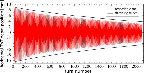
Refer to caption

Figure 23: (Color) Example of horizontal turn-by-turn beam oscillation after the pulse of an horizontal kicker magnet measured at the ESRF electron storage ring. A special sextupole setting was used to minimize amplitude-dependent detuning and chromaticity. The decreasing amplitude is believed to be the result of radiation damping (black curve, damping time of 7 ms, corresponding to about 2500 turns).

Refer to caption

Refer to caption

Figure 24: (Color) Example of horizontal turn-by-turn spectra measured at the ESRF electron storage ring. The upper plots are the FFT of the real signal x~(N)=x(N)/βx~𝑥𝑁𝑥𝑁subscript𝛽𝑥\tilde{x}(N)=x(N)/\sqrt{\beta_{x}} computed over 1024 and 512 turns, respectively. Despite the longer signal, the spectrum with 1024 turns shows higher background noise, which is attributed to radiation damping. In both cases, the region [0.5,1] is the mirrored copy (i.e. complex conjugate) of the region [0,0.5]. The bottom plot shows the FFT over 512 turns of the complex signal hx(N)=x~(N)ip~x(N)subscript𝑥𝑁~𝑥𝑁𝑖subscript~𝑝𝑥𝑁h_{x}(N)=\tilde{x}(N)-i\tilde{p}_{x}(N): There is no mirroring around 0.5, but the background noise is higher than in the simple FFT of x~~𝑥\tilde{x} (center plot) and some spectral lines are no longer visible. For a complete (up to the first order) classification of all spectral lines, see Table IV of Ref. prstab_strength .

Another aspect limiting the applicability of the multi-BPM signals in electron machine is represented by radiation damping. Ideally, the greater the number of turns with exploitable data (i.e. before decoherence smooths out the signal to zero), the higher the spectral resolution and hence the quality of the RDT measurement. At the ESRF a special sextupole setting was found to provide low amplitude-dependent detuning and linear chromaticity in both planes, so to minimize decoherence. However, the damping time being of about 2500 turns, the signal is sufficiently depressed to compromise the whole measurement already after 1024 turns (see Fig. 23). It has been observed that the spectral background noise increases with the number of turns used to perform the FFT of the turn-by-turn signal (see upper plots of Fig. 24): An effect which is believed to be related to radiation damping. Moreover, when analyzing the complex signal hxsubscript𝑥h_{x} constructed between two consecutive BPMs the background noise is enhanced (see bottom plot of Fig. 24). The sextupolar spectral lines being intrinsically of limited height, it is of capital interest to keep the spectral background noise as low as possible, so to enhance the signal-to-noise ratio. For this reason, even if 2048 turns may be stored by each BPM, only 256 or 512 are routinely used at the ESRF in order to carry out the harmonic analysis, a trade off between enhancement of spectral resolution and minimization background noise.

A new approach has been then developed to measure (a different kind of) RDTs from single-BPM data, r~(N)=r(N)/βr~𝑟𝑁𝑟𝑁subscript𝛽𝑟\tilde{r}(N)=r(N)/\sqrt{\beta_{r}}, in order to avoid the noise enhancement whenever data from two or three BPMs are used. By using single-BPM data the issue of synchronization between the monitors is no longer of concern, the harmonic analysis at each BPM being independent of the data acquired by the others.

The bottom plot of Fig. 24 shows a typical horizontal spectrum of hxsubscript𝑥h_{x} with the excited spectral lines: Besides the principal tune line generated by the main quadrupoles, quadrupole errors (beta-beat) excite a line at the frequency 1Qx1subscript𝑄𝑥1-Q_{x}, Hh(1,0)subscript𝐻10H_{h}(-1,0), while betatron coupling is visible from the presence of a secondary line at the frequency corresponding to the vertical tune, Hh(0,1)subscript𝐻01H_{h}(0,1), and its reciprocal, Hh(1,0)subscript𝐻10H_{h}(-1,0). The main sextupoles (chromatic and harmonic) generate several lines, among which Hh(±2,0)subscript𝐻plus-or-minus20H_{h}(\pm 2,0) and Hh(0,±2)subscript𝐻0plus-or-minus2H_{h}(0,\pm 2). Skew sextupole lines appear also at the position QxQysubscript𝑄𝑥subscript𝑄𝑦Q_{x}-Q_{y}, Hh(1,1)subscript𝐻11H_{h}(1,-1), and 1QxQy1subscript𝑄𝑥subscript𝑄𝑦1-Q_{x}-Q_{y}, Hh(1,1)subscript𝐻11H_{h}(-1,-1): their origin will be discussed later. Other lines generated by 2-nd order sextupolar terms are more visible in the spectrum of x~~𝑥\tilde{x} (center plot of Fig. 24).

The harmonic analysis of the real signal r~~𝑟\tilde{r} produces a spectrum that is mirrored around 0.5 (in tune units). By looking at Table IV of Ref. prstab_strength and Fig. 24 it is clear that secondary spectral lines of the complex signal hrsubscript𝑟h_{r} and excited by either coupling or sextupoles, become indistinguishable. For instance, the two sextupolar horizontal spectral lines Hh(2,0)subscript𝐻20H_{h}(2,0), located at the frequency 2Qx2subscript𝑄𝑥2Q_{x}, and Hh(2,0)subscript𝐻20H_{h}(-2,0), located at 12Qx12subscript𝑄𝑥1-2Q_{x}, are excited by the two different RDTs, f1200subscript𝑓1200f_{1200} and f3000subscript𝑓3000f_{3000}, respectively. The latter are distinguishable and measurable from the FFT of the complex signal hxsubscript𝑥h_{x}, while the mirroring around 0.5 prevents such distinction if the FFT is performed on the real signal x~~𝑥\tilde{x}. An example may help understanding this merging. A complex signal hxsubscript𝑥h_{x} contains two harmonics in the following combination

hx(N)=A+ei(4πQxN+ψ)+Aei(4πQxN+θ).subscript𝑥𝑁subscript𝐴superscript𝑒𝑖4𝜋𝑄𝑥𝑁𝜓subscript𝐴superscript𝑒𝑖4𝜋𝑄𝑥𝑁𝜃\displaystyle h_{x}(N)=A_{+}e^{i(4\pi QxN+\psi)}+A_{-}e^{i(-4\pi QxN+\theta)}\ .

The first term would correspond ideally at the spectral line Hh(2,0)subscript𝐻20H_{h}(2,0), while the second to Hh(2,0)subscript𝐻20H_{h}(-2,0). The FFT of hx(N)subscript𝑥𝑁h_{x}(N) would yield two spectral lines located at 2Qx2subscript𝑄𝑥2Q_{x} and 12Qx12subscript𝑄𝑥1-2Q_{x}, respectively, with measurable amplitudes (A+subscript𝐴A_{+} and Asubscript𝐴A_{-}) and phases (ψ𝜓\psi and θ𝜃\theta). The real part of hx(N)subscript𝑥𝑁h_{x}(N), corresponding to the single-BPM turn-by-turn data x~~𝑥\tilde{x}, reads

x~~𝑥\displaystyle\tilde{x} =\displaystyle= {hx}(N)subscript𝑥𝑁\displaystyle\Re\{h_{x}\}(N)
=\displaystyle= A+ei(4πQxN+ψ)+ei(4πQxN+ψ)2+limit-fromsubscript𝐴superscript𝑒𝑖4𝜋𝑄𝑥𝑁𝜓superscript𝑒𝑖4𝜋𝑄𝑥𝑁𝜓2\displaystyle A_{+}\frac{e^{i(4\pi QxN+\psi)}+e^{-i(4\pi QxN+\psi)}}{2}+
Aei(4πQxN+θ)+ei(4πQxNθ)2subscript𝐴superscript𝑒𝑖4𝜋𝑄𝑥𝑁𝜃superscript𝑒𝑖4𝜋𝑄𝑥𝑁𝜃2\displaystyle A_{-}\frac{e^{i(-4\pi QxN+\theta)}+e^{i(4\pi QxN-\theta)}}{2}
=\displaystyle= [A+eiψ+Aeiθ]2ei4πQxN+c.c..formulae-sequencedelimited-[]subscript𝐴superscript𝑒𝑖𝜓subscript𝐴superscript𝑒𝑖𝜃2superscript𝑒𝑖4𝜋𝑄𝑥𝑁𝑐𝑐\displaystyle\frac{\left[A_{+}e^{i\psi}+A_{-}e^{-i\theta}\right]}{2}e^{i4\pi QxN}+c.c.\qquad.

The omitted term represents the complex conjugate of the first (i.e. its mirrored copy) and contains no additional information. The FFT of x~(N)~𝑥𝑁\tilde{x}(N) would still generate two spectral lines H(±2,0)𝐻plus-or-minus20H(\pm 2,0), which are however complex conjugates. This implies that the only (complex) observable left is [A+eiψ+Aeiθ]delimited-[]subscript𝐴superscript𝑒𝑖𝜓subscript𝐴superscript𝑒𝑖𝜃\left[A_{+}e^{i\psi}+A_{-}e^{-i\theta}\right], while the four quantities A±subscript𝐴plus-or-minusA_{\pm}, ψ𝜓\psi and θ𝜃\theta are no longer measurable. Back to the RDT context, the consequence of analyzing the single-BPM signal instead of hrsubscript𝑟h_{r} is that only linear combinations of RDTs are directly measurable. It will be shown that this is still sufficient to infer lattice errors and provide a correction scheme.

Generally speaking, each line in the spectrum of x~(N)~𝑥𝑁\tilde{x}(N) is the superposition of two lines in the spectrum of hx(N)subscript𝑥𝑁h_{x}(N), according to

H(nx,ny)=[Hh(nx,ny)+Hh(nx,ny)]2.𝐻subscript𝑛𝑥subscript𝑛𝑦delimited-[]subscript𝐻subscript𝑛𝑥subscript𝑛𝑦subscript𝐻subscript𝑛𝑥subscript𝑛𝑦2\displaystyle H(n_{x},n_{y})=\frac{\left[H_{h}(n_{x},n_{y})+H_{h}(-n_{x},-n_{y})\right]}{2}\ . (129)

H(nx,ny)𝐻subscript𝑛𝑥subscript𝑛𝑦H(n_{x},n_{y}) without suffix denotes a line in spectrum of the real signal x~(N)~𝑥𝑁\tilde{x}(N). Hh(nx,ny)subscript𝐻subscript𝑛𝑥subscript𝑛𝑦H_{h}(n_{x},n_{y}) refers to a generic line in the spectrum of the complex signal hx(n)subscript𝑥𝑛h_{x}(n). Identical relations hold for the vertical spectrum.

Appendix C Quadrupole errors and tune-line amplitude

In Table 2 (easier) first-order RDTs fjklmsubscript𝑓𝑗𝑘𝑙𝑚f_{jklm} for skew quadrupole and normal sextupole spectral lines are used, while for skew sextupoles (more complex) second-order ORDTs gjklmsubscript𝑔𝑗𝑘𝑙𝑚g_{jklm} are invoked. The latter are also used in Table 9 for normal octupoles. In this section motivations and conditions for such a choice are provided. It will be shown how this is related to the removal of RDTs generated by focusing errors when using the modulated beta functions (i.e. computed from a lattice including quadrupole errors) rather than those of the ideal lattice.

Parenthetically, a novel procedure for using single-BPM turn-by-turn data to measure the beta functions is described, which is complementary to the traditional approach based on the direct measurement of the phase advance between two consecutive BPMs Castro . The latter is independent on calibration errors, but requires a perfect synchronization among the BPMs. The proposed scheme, on the contrary, necessitates well calibrated monitors but does not need any synchronization, as for the nonlinear analysis of Table 2.

In the Appendix of Ref. prstab_coup the complete Lie series of Eq. (108) was computed in presence of betatron coupling, i.e. with the normal form transformation F𝐹F defined exclusively by coupling RDTs, namely

F=𝐹absent\displaystyle F= f1001ζx,+ζy,+f1001ζx,ζy,++f1010ζx,+ζy,+subscript𝑓1001subscript𝜁𝑥subscript𝜁𝑦superscriptsubscript𝑓1001subscript𝜁𝑥subscript𝜁𝑦subscript𝑓1010subscript𝜁𝑥subscript𝜁𝑦\displaystyle f_{1001}\zeta_{x,+}\zeta_{y,-}+f_{1001}^{*}\zeta_{x,-}\zeta_{y,+}+f_{1010}\zeta_{x,+}\zeta_{y,+} (130)
+f1010ζxζy.superscriptsubscript𝑓1010superscriptsubscript𝜁𝑥superscriptsubscript𝜁𝑦\displaystyle\hskip 14.22636pt+f_{1010}^{*}\zeta_{x}^{-}\zeta_{y}^{-}\ .

Recursive expressions for the Poisson brackets at any order were derived leading to the following expression for the turn-by-turn evolution of the complex Courant-Snyder coordinates

hxsubscript𝑥\displaystyle h_{x} =\displaystyle= cosh(2𝒫)ζx,isinh(2𝒫)[f1001𝒫ζy,+f1010𝒫ζy,+]2𝒫subscript𝜁𝑥𝑖2𝒫delimited-[]subscript𝑓1001𝒫subscript𝜁𝑦subscript𝑓1010𝒫subscript𝜁𝑦\displaystyle\hskip-1.42271pt\cosh{(2\mathcal{P})}\ \zeta_{x,-}-\hskip-2.84544pti\sinh{(2\mathcal{P})}\left[\frac{f_{1001}}{\mathcal{P}}\zeta_{y,-}+\frac{f_{1010}}{\mathcal{P}}\zeta_{y,+}\right]\hskip-2.84544pt
\displaystyle\hskip 14.22636pt\Uparrow\hskip 113.81102pt\Uparrow\hskip 48.36958pt\Uparrow
Hh(1,0)Hh(0,1)Hh(0,1)subscript𝐻10subscript𝐻01subscript𝐻01\displaystyle\hskip 5.69046ptH_{h}(1,0)\hskip 79.6678ptH_{h}(0,1)\hskip 14.22636ptH_{h}(0,-1)
hysubscript𝑦\displaystyle h_{y} =\displaystyle= cosh(2𝒫)ζy,isinh(2𝒫)[f1001𝒫ζx,+f1010𝒫ζx,+]2𝒫subscript𝜁𝑦𝑖2𝒫delimited-[]subscriptsuperscript𝑓1001𝒫subscript𝜁𝑥subscript𝑓1010𝒫subscript𝜁𝑥\displaystyle\hskip-1.42271pt\cosh{(2\mathcal{P})}\ \zeta_{y,-}-\hskip-2.84544pti\sinh{(2\mathcal{P})}\left[\frac{f^{*}_{1001}}{\mathcal{P}}\zeta_{x,-}+\frac{f_{1010}}{\mathcal{P}}\zeta_{x,+}\right]\hskip-2.84544pt
\displaystyle\hskip 14.22636pt\Uparrow\hskip 113.81102pt\Uparrow\hskip 48.36958pt\Uparrow
Vh(0,1)Vh(1,0)Vh(1,0)subscript𝑉01subscript𝑉10subscript𝑉10\displaystyle\hskip 5.69046ptV_{h}(0,1)\hskip 79.6678ptV_{h}(1,0)\hskip 19.91684ptV_{h}(-1,0)

where

2𝒫2𝒫\displaystyle 2\mathcal{P} =\displaystyle= |2f1001|2+|2f1010|2.superscript2subscript𝑓10012superscript2subscript𝑓10102\displaystyle\sqrt{-|2f_{1001}|^{2}+|2f_{1010}|^{2}}\ . (133)

According to Eq. (129) the tune lines of the real Courant-Snyder coordinates read

H(1,0)𝐻10\displaystyle H(1,0) =\displaystyle= cosh(2𝒫)22Ixei(2πNQx+ψx,0)+c.c.,formulae-sequence2𝒫22subscript𝐼𝑥superscript𝑒𝑖2𝜋𝑁subscript𝑄𝑥subscript𝜓𝑥0𝑐𝑐\displaystyle\frac{\cosh{(2\mathcal{P})}}{2}\sqrt{2I_{x}}e^{i(2\pi NQ_{x}+\psi_{x,0})}+c.c.\quad,\qquad (134)
V(0,1)𝑉01\displaystyle V(0,1) =\displaystyle= cosh(2𝒫)22Iyei(2πNQy+ψy,0)+c.c.,formulae-sequence2𝒫22subscript𝐼𝑦superscript𝑒𝑖2𝜋𝑁subscript𝑄𝑦subscript𝜓𝑦0𝑐𝑐\displaystyle\frac{\cosh{(2\mathcal{P})}}{2}\sqrt{2I_{y}}e^{i(2\pi NQ_{y}+\psi_{y,0})}+c.c.\quad,\qquad (135)

where c.c.formulae-sequence𝑐𝑐c.c. stands for complex conjugate. Note that in presence of pure coupling Hh(1,0)=Vh(0,1)=0subscript𝐻10subscript𝑉010H_{h}(-1,0)=V_{h}(0,-1)=0.

The same algebra may be applied to another extreme case with normal quadrupole errors only, i.e. with the normal form transformation F𝐹F defined exclusively by focusing error RDTs

F=f2000ζx,+2+f2000ζx,2+f0020ζy,+2+f0020ζy,2.𝐹subscript𝑓2000superscriptsubscript𝜁𝑥2superscriptsubscript𝑓2000superscriptsubscript𝜁𝑥2subscript𝑓0020superscriptsubscript𝜁𝑦2superscriptsubscript𝑓0020superscriptsubscript𝜁𝑦2\displaystyle F=f_{2000}\zeta_{x,+}^{2}+f_{2000}^{*}\zeta_{x,-}^{2}+f_{0020}\zeta_{y,+}^{2}+f_{0020}^{*}\zeta_{y,-}^{2}\ .\qquad (136)

The result is

hxsubscript𝑥\displaystyle h_{x} =\displaystyle= cosh(4|f2000|)ζx,isinh(4|f2000|)eiq2000ζx,+,4subscript𝑓2000subscript𝜁𝑥𝑖4subscript𝑓2000superscript𝑒𝑖subscript𝑞2000subscript𝜁𝑥\displaystyle\cosh{(4|f_{2000}|)}\ \zeta_{x,-}-i\sinh{(4|f_{2000}|)}\ e^{iq_{2000}}\ \zeta_{x,+}\ ,
absent\displaystyle\hskip 42.67912pt\Uparrow\hskip 102.43008pt\Uparrow
Hh(1,0)Hh(1,0)subscript𝐻10subscript𝐻10\displaystyle\hskip 34.14322ptH_{h}(1,0)\hskip 62.59596ptH_{h}(-1,0)
hysubscript𝑦\displaystyle h_{y} =\displaystyle= cosh(4|f0020|)ζy,isinh(4|f0020|)eiq0020ζy,+,4subscript𝑓0020subscript𝜁𝑦𝑖4subscript𝑓0020superscript𝑒𝑖subscript𝑞0020subscript𝜁𝑦\displaystyle\cosh{(4|f_{0020}|)}\ \zeta_{y,-}-i\sinh{(4|f_{0020}|)}\ e^{iq_{0020}}\ \zeta_{y,+}\ ,
absent\displaystyle\hskip 42.67912pt\Uparrow\hskip 102.43008pt\Uparrow
Vh(0,1)Vh(0,1)subscript𝑉01subscript𝑉01\displaystyle\hskip 34.14322ptV_{h}(0,1)\hskip 62.59596ptV_{h}(0,-1)

where

q2000subscript𝑞2000\displaystyle q_{2000} =\displaystyle= arg{f2000}andq0020=arg{f0020},argsubscript𝑓2000andsubscript𝑞0020argsubscript𝑓0020\displaystyle\hbox{arg}\left\{f_{2000}\right\}\quad\hbox{and}\quad q_{0020}=\hbox{arg}\left\{f_{0020}\right\}\ ,\qquad (139)
f2000subscript𝑓2000\displaystyle f_{2000} =\displaystyle= wWδKw,1βxwe2iΔϕw,x8(1e4πiQx),superscriptsubscript𝑤𝑊𝛿subscript𝐾𝑤1superscriptsubscript𝛽𝑥𝑤superscript𝑒2𝑖Δsubscriptitalic-ϕ𝑤𝑥81superscript𝑒4𝜋𝑖subscript𝑄𝑥\displaystyle\frac{\sum\limits_{w}^{W}\delta K_{w,1}\beta_{x}^{w}e^{2i\Delta\phi_{w,x}}}{8(1-e^{4\pi iQ_{x}})}\ , (140)
f0020subscript𝑓0020\displaystyle f_{0020} =\displaystyle= wWδKw,1βywe2iΔϕw,y8(1e4πiQy),superscriptsubscript𝑤𝑊𝛿subscript𝐾𝑤1superscriptsubscript𝛽𝑦𝑤superscript𝑒2𝑖Δsubscriptitalic-ϕ𝑤𝑦81superscript𝑒4𝜋𝑖subscript𝑄𝑦\displaystyle\frac{\sum\limits_{w}^{W}\delta K_{w,1}\beta_{y}^{w}e^{2i\Delta\phi_{w,y}}}{8(1-e^{4\pi iQ_{y}})}\ , (141)

with βx,ysubscript𝛽𝑥𝑦\beta_{x,y} and Δϕx,yΔsubscriptitalic-ϕ𝑥𝑦\Delta\phi_{x,y} are the the C-S parameters of the ideal lattice (i.e. without focusing errors δKw,1𝛿subscript𝐾𝑤1\delta K_{w,1}). Conversely to coupling, pure quadrupole errors excite directly the two lines Hh(1,0)subscript𝐻10H_{h}(-1,0) and Vh(0,1)subscript𝑉01V_{h}(0,-1). Applying again Eq. (129) the tune lines of the real Courant-Snyder coordinates read

H(1,0)𝐻10\displaystyle H(1,0) =\displaystyle= 12[cosh(4|f2000|)+isinh(4|f2000|)eiq2000]12delimited-[]4subscript𝑓2000𝑖4subscript𝑓2000superscript𝑒𝑖subscript𝑞2000\displaystyle\frac{1}{2}\Big{[}\cosh{(4|f_{2000}|)}+i\sinh{(4|f_{2000}|)}e^{-iq_{2000}}\Big{]} (142)
×2Ixei(2πNQx+ψx,0)+c.c.,\displaystyle\hskip 28.45274pt\times\sqrt{2I_{x}}e^{i(2\pi NQ_{x}+\psi_{x,0})}+c.c.\quad,\qquad
V(0,1)𝑉01\displaystyle V(0,1) =\displaystyle= 12[cosh(4|f0020|)+isinh(4|f0020|)eiq0020]12delimited-[]4subscript𝑓0020𝑖4subscript𝑓0020superscript𝑒𝑖subscript𝑞0020\displaystyle\frac{1}{2}\Big{[}\cosh{(4|f_{0020}|)}+i\sinh{(4|f_{0020}|)}e^{-iq_{0020}}\Big{]} (143)
×2Iyei(2πNQy+ψy,0)+c.c.,\displaystyle\hskip 28.45274pt\times\sqrt{2I_{y}}e^{i(2\pi NQ_{y}+\psi_{y,0})}+c.c.\quad,\qquad

In the more general case with both quadrupole and coupling errors similar results may be derived. However, Eqs. (134)-(135) and (142)-(143) already reveal an intrinsic feature of linear lattice errors: The amplitude of the tune lines H(1,0)𝐻10H(1,0) and V(0,1)𝑉01V(0,1) are modified by the RDTs. The implication of that is twofold. First, it becomes impossible to use single-BPM turn-by-turn data to disentangle and measure coupling and beta-beat RDTs, because the tune lines used to extract them from the secondary lines in Refs. Rogelio1 ; Andrea-thesis ; prstab_strength depend on the RDTs too. For the same reason, measurement of sextupolar combined RDTs of Table 2 will be corrupted.

A way out from this inconvenient situation is represented by measuring (and correcting) lattice errors before carrying out the turn-by-turn analysis with an independent technique, such as the orbit response matrix (ORM) and LOCO analysis of Ref. ORM . In Ref. prstab_esr_coupling the procedure to evaluate first-order focusing and coupling RDTs from ORM measurement is described in detail. It can be hence assumed that f2000subscript𝑓2000f_{2000}, f0020subscript𝑓0020f_{0020}, f1001subscript𝑓1001f_{1001}, and f1010subscript𝑓1010f_{1010} be known prior to the turn-by-turn analysis. At the ESRF, with (peak) beta-beating usually corrected up to ±5%plus-or-minuspercent5\pm 5\% and betatron coupling so to have an emittance ratio lower than 111‰, typical values of 𝒫𝒫\mathcal{P}, |f2000|subscript𝑓2000|f_{2000}| and |f0020|subscript𝑓0020|f_{0020}| are lower than 102superscript10210^{-2}, see Fig. 25. Hence the perturbation introduced by coupling to the tune-line amplitudes of Eqs. (134) and (135) is negligible, 1cosh(2𝒫)<10412𝒫superscript1041-\cosh{(2\mathcal{P})}<10^{-4}. The same is true only partially for quadrupole errors: while 1cosh(4|f2000|)1cosh(4|f0020|)<104similar-to-or-equals14subscript𝑓200014subscript𝑓0020superscript1041-\cosh{(4|f_{2000}|)}\simeq 1-\cosh{(4|f_{0020}|)}<10^{-4}, the residual modulation introduced by the hyperbolic sines in Eqs. (142) and (143) may not be ignored, remaining of the level of percents. If such a modulation is not removed, it will be propagated as an error in the nonlinear error model.
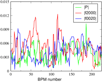
Refer to caption

Figure 25: (Color) Comparison between the coupling RDT factor 𝒫𝒫\mathcal{P} (green) and the focusing error RDTs f2000subscript𝑓2000f_{2000} (red), f0020subscript𝑓0020f_{0020} (blue) inferred from ORM measurement at the ESRF electron storage ring after correction (peak beta-beating of about ±5%plus-or-minuspercent5\pm 5\% and an emittance ration lower than 111‰). All three quantities are of the same order of magnitude, though well below 102superscript10210^{-2} level.

The task of making the tune-line amplitudes constant along the ring is actually much easier than it may appear. From Eq. (142) (the same applies to the vertical plane) the tune-line amplitude reads

|H(1,0)|𝐻10\displaystyle|H(1,0)| =\displaystyle= 2Ix2{1+2sinh(4|f2000|)×\displaystyle\frac{\sqrt{2I_{x}}}{2}\Bigg{\{}1+2\sinh{(4|f_{2000}|)}\times
[sinh(4|f2000|)+cosh(4|f2000|)sinq2000]}1/2.\displaystyle\hskip-14.22636pt\Big{[}\sinh{(4|f_{2000}|)}+\cosh{(4|f_{2000}|)}\sin{q_{2000}}\Big{]}\Bigg{\}}^{1/2}\ .

In the ideal lattice, the Courant-Snyder coordinate x~=x/βx~𝑥𝑥subscript𝛽𝑥\tilde{x}=x/\sqrt{\beta_{x}} would provide a a tune-line amplitude

|H(1,0)|0subscript𝐻100\displaystyle|H(1,0)|_{0} =\displaystyle= 2Ix2.2subscript𝐼𝑥2\displaystyle\frac{\sqrt{2I_{x}}}{2}\ . (145)

It is straightforward to prove that by scaling the beta function by a factor c𝑐c, βx1=cβxsubscript𝛽𝑥1𝑐subscript𝛽𝑥\beta_{x1}=c\beta_{x}, the tune-line amplitude scales as

|H(1,0)|𝐻10\displaystyle|H(1,0)| =\displaystyle= 1c2Ix2.1𝑐2subscript𝐼𝑥2\displaystyle\frac{1}{\sqrt{c}}\frac{\sqrt{2I_{x}}}{2}\ . (146)

Hence, it is enough to replace the ideal beta function βxsubscript𝛽𝑥\beta_{x} with

βx1subscript𝛽𝑥1\displaystyle\beta_{x1} =\displaystyle= βx{1+2sinh(4|f2000|)[sinh(4|f2000|)\displaystyle\beta_{x}\Bigg{\{}1+2\sinh{(4|f_{2000}|)}\Big{[}\sinh{(4|f_{2000}|)} (147)
+cosh(4|f2000|)sinq2000]}\displaystyle\hskip 28.45274pt+\cosh{(4|f_{2000}|)}\sin{q_{2000}}\Big{]}\Bigg{\}}

to retrieve a RDT-independent tune line, |H(1,0)|=2Ix/2𝐻102subscript𝐼𝑥2|H(1,0)|=\sqrt{2I_{x}}/2. Equation (147) provides an analytical expression for the horizontal beta-beating introduced by quadrupole errors:

ΔβxβxΔsubscript𝛽𝑥subscript𝛽𝑥\displaystyle\frac{\Delta\beta_{x}}{\beta_{x}} =\displaystyle= 2sinh(4|f2000|)[sinh(4|f2000|)\displaystyle 2\sinh{(4|f_{2000}|)}\Big{[}\sinh{(4|f_{2000}|)}
+cosh(4|f2000|)sinq2000].\displaystyle\hskip 73.97733pt+\cosh{(4|f_{2000}|)}\sin{q_{2000}}\Big{]}\ .

The same algebra applied to the vertical plane leads to

ΔβyβyΔsubscript𝛽𝑦subscript𝛽𝑦\displaystyle\frac{\Delta\beta_{y}}{\beta_{y}} =\displaystyle= 2sinh(4|f0020|)[sinh(4|f0020|)\displaystyle 2\sinh{(4|f_{0020}|)}\Big{[}\sinh{(4|f_{0020}|)}
+cosh(4|f0020|)sinq0020].\displaystyle\hskip 73.97733pt+\cosh{(4|f_{0020}|)}\sin{q_{0020}}\Big{]}\ .

In Fig.26 a comparison between the beta-beating as computed by MADX and by Eqs. (C) and (C) is shown. The lattice error model loaded in MADX is derived from an ORM measurement carried out at the ESRF storage ring. First-order RDTs f2000subscript𝑓2000f_{2000} and f0020subscript𝑓0020f_{0020} may be computed from the focusing errors via Eqs. (140) and (141). For a more accurate comparison, the RDTs used in Fig.26 are inferred from the harmonic analysis of single-particle tracking data, after isolating the Hh(1,0)subscript𝐻10H_{h}(-1,0) and Vh(0,1)subscript𝑉01V_{h}(0,-1) of Eqs. (C) and (C). The agreement is remarkable.
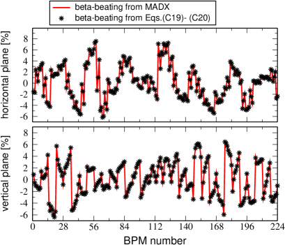
Refer to caption

Figure 26: (Color) Comparison between the beta-beating computed by MADX after loading an error model constructed from an ORM measurement at the ESRF storage ring (red) and that evaluated from Eqs (C) and (C) (black stars).

In practice then, the perturbations introduced by the focusing error RDTs f2000subscript𝑓2000f_{2000} and f0020subscript𝑓0020f_{0020} of Eqs. (140) and (141) may be absorbed by replacing the ideal C-S parameters βx,ysubscript𝛽𝑥𝑦\beta_{x,y} and Δϕx,yΔsubscriptitalic-ϕ𝑥𝑦\Delta\phi_{x,y} with the modulated ones βx1,y1subscript𝛽𝑥1𝑦1\beta_{x1,y1} and Δϕx1,y1Δsubscriptitalic-ϕ𝑥1𝑦1\Delta\phi_{x1,y1}. By doing so, the new Courant-Snyder coordinates will no longer show quadrupole errors, and the beta-beat RDTs vanish, i.e.

f2000(βx,Δϕx)subscript𝑓2000subscript𝛽𝑥Δsubscriptitalic-ϕ𝑥\displaystyle f_{2000}(\beta_{x},\Delta\phi_{x}) \displaystyle\neq 0butf2000(βx1,Δϕx1)0,0butsubscript𝑓2000subscript𝛽𝑥1Δsubscriptitalic-ϕ𝑥10\displaystyle 0\quad\hbox{but}\quad f_{2000}(\beta_{x1},\Delta\phi_{x1})\equiv 0\ ,\qquad (150)
f0020(βy,Δϕy)subscript𝑓0020subscript𝛽𝑦Δsubscriptitalic-ϕ𝑦\displaystyle f_{0020}(\beta_{y},\Delta\phi_{y}) \displaystyle\neq 0butf0020(βx1,Δϕx1)0.0butsubscript𝑓0020subscript𝛽𝑥1Δsubscriptitalic-ϕ𝑥10\displaystyle 0\quad\hbox{but}\quad f_{0020}(\beta_{x1},\Delta\phi_{x1})\equiv 0\ .\qquad (151)

Physically this corresponds to the fact that not including focusing errors in the computation of the C-S parameters results in mismatched functions and a phase space topology (ellipses) dependent on the longitudinal position along the ring (through the s𝑠s-dependent beta-beating RDTs f2000subscript𝑓2000f_{2000} and f0020subscript𝑓0020f_{0020}). When, instead, the C-S parameters used to compute the C-S coordinates properly account for all normal quadrupole forces, the corresponding phase space topology becomes invariant along the ring (and circular).

Even though focusing errors and coupling may be efficiently measured and corrected from ORM measurement, the inferred model results usually from a best fit procedure which converges towards the measured matrix up to a certain degree of precision. Provided that coupling is well corrected (e.g. cosh(2𝒫)=12𝒫1\cosh{(2\mathcal{P})}=1 up to a sufficient level), the same single-BPM turn-by-turn data may be used to validate and possibly to further correct the beta functions. The starting point are focusing RDTs that, despite the use of C-S parameters obtained from the error model, may still be nonzero because of residual fit errors, i.e. 0f2000(βx,Δϕx),f0020(βx,Δϕx)1formulae-sequence0subscript𝑓2000subscript𝛽𝑥Δsubscriptitalic-ϕ𝑥much-less-thansubscript𝑓0020subscript𝛽𝑥Δsubscriptitalic-ϕ𝑥10\neq f_{2000}(\beta_{x},\Delta\phi_{x}),\ f_{0020}(\beta_{x},\Delta\phi_{x})\ll 1. It is then reasonable to assume that cosh(4|f2000|)cosh(4|f0020|)=1similar-to-or-equals4subscript𝑓20004subscript𝑓00201\cosh{(4|f_{2000}|)}\simeq\cosh{(4|f_{0020}|)}=1 up to a sufficient level of tolerance. Equation (C) then simplifies to

|H(1,0)|=2Ix2{1+8|f2000|sinq2000+O(|f2000|2)}1/2.𝐻102subscript𝐼𝑥2superscript18subscript𝑓2000subscript𝑞2000𝑂superscriptsubscript𝑓2000212\displaystyle|H(1,0)|=\frac{\sqrt{2I_{x}}}{2}\Big{\{}1+8|f_{2000}|\sin{q_{2000}}+O(|f_{2000}|^{2})\Big{\}}^{1/2}.
(152)

The above expression contains a constant term, 2Ix/22subscript𝐼𝑥2\sqrt{2I_{x}}/2, and an oscillating one proportional to the residual focusing RDT, |f2000|sinq2000subscript𝑓2000subscript𝑞2000|f_{2000}|\sin{q_{2000}}. If the number of oscillations along the ring is sufficiently large and the number of BPM enough to cover uniformly the path, by averaging the tune-line amplitudes among all BPMs, the oscillating term cancels out and the invariant may be retrieved:

2Ix21Nn=1N|H(1,0)|n,similar-to-or-equals2subscript𝐼𝑥21𝑁superscriptsubscript𝑛1𝑁subscript𝐻10𝑛\displaystyle\sqrt{2I_{x}}\simeq 2\frac{1}{N}\sum_{n=1}^{N}{|H(1,0)|_{n}}\ , (153)
2Iy21Nn=1N|V(0,1)|n,similar-to-or-equals2subscript𝐼𝑦21𝑁superscriptsubscript𝑛1𝑁subscript𝑉01𝑛\displaystyle\sqrt{2I_{y}}\simeq 2\frac{1}{N}\sum_{n=1}^{N}{|V(0,1)|_{n}}\ , (154)

where N𝑁N is the number of available BPMs (not necessarily synchronized over the same turns and/or bunches) and |H(1,0)|nsubscript𝐻10𝑛|H(1,0)|_{n} are the tune-line amplitudes measured at the different monitors. More intriguingly, the same single-BPM turn-by-turn data may be post-processed to extract the true beta function at its location. Once the average tune-line amplitude is computed, <|H(1,0)|>absent𝐻10absent<|H(1,0)|> (<|V(0,1)|>absent𝑉01absent<|V(0,1)|>), at each BPM the beta function may be scaled by a factor c=[|H(1,0)|n/<|H(1,0)|>]2𝑐superscriptdelimited-[]subscript𝐻10𝑛expectation𝐻102c=[\ |H(1,0)|_{n}/<|H(1,0)|>]^{2} (c=[|V(0,1)|n/<|V(0,1)|>]2𝑐superscriptdelimited-[]subscript𝑉01𝑛expectation𝑉012c=[\ |V(0,1)|_{n}/<|V(0,1)|>]^{2}) as done for Eq. (147). The result is then straightforward:

βx1,n=(|H(1,0)|n<|H(1,0)|>)2βx,n,subscript𝛽𝑥1𝑛superscriptsubscript𝐻10𝑛absent𝐻10absent2subscript𝛽𝑥𝑛\displaystyle\beta_{x1,n}=\left(\frac{|H(1,0)|_{n}}{<|H(1,0)|>}\right)^{2}\beta_{x,n}\ , (155)
βy1,n=(|V(0,1)|n<|V(0,1)|>)2βy,n,subscript𝛽𝑦1𝑛superscriptsubscript𝑉01𝑛absent𝑉01absent2subscript𝛽𝑦𝑛\displaystyle\beta_{y1,n}=\left(\frac{|V(0,1)|_{n}}{<|V(0,1)|>}\right)^{2}\beta_{y,n}\ , (156)

where βx,nsubscript𝛽𝑥𝑛\beta_{x,n} denotes the initial horizontal beta function obtained from the lattice error model created, for instance, from the ORM measurement and fit, while βx1,nsubscript𝛽𝑥1𝑛\beta_{x1,n} are those corrected by the harmonic turn-by-turn analysis.
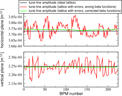
Refer to caption

Refer to caption

Figure 27: (Color) Top: Evolution of the tune-line amplitudes along the SERF storage ring obtained from single-particle tracking with the ideal lattice (black curve), with lattice errors included in the tracking but not in the beta functions (red), and with the beta functions corrected after minimizing the spread between the tune-line amplitudes among the BPMs (green). Bottom: Comparison between the expected beta-beating as computed by MADX (magenta curve) and the once inferred from the minimization of the spread among the tune-line amplitudes (black stars). Note how the tune-line amplitude pattern (red curve, upper plot) matches that of the beta-beating (bottom plot).

In Fig. 27 the results from a numerical test carried out from single-particle tracking with the same focusing errors and coupling of Fig. 25 is shown. Single-BPM turn-by-turn data are represented by the particle coordinates stored at the 224 BPMs of the ESRF storage ring for 256 turns. The Courant-Snyder variable is constructed from the ideal beta functions (hence without including the focusing errors). Once the average tune-line amplitude is computed, the new beta functions are computed from the ratio between the tune-line amplitude at the BPM and the mean value. The resulting beta-beating is compared with the one computed by MADX confirming the excellent agreement, while the spread between the tune-line amplitude evaluated at the 224 BPMs with the new beta functions drops dramatically. Note how the tune-line amplitude pattern (red curve in the upper plot) matches that of the beta-beating (bottom plot).

The use of the C-S parameters that already include focusing errors in evaluating the first-order RDTs of Table 3 not only will correctly account for the modulation introduced by the beta functions βx,ysubscript𝛽𝑥𝑦\beta_{x,y}, but has a tremendous impact in simplifying the second-order analysis of coupling and normal sextupole RDTs of Tables 13 and 13, respectively: The first-order beta-beat RDTs being all zero (as well as the corresponding Hamiltonian coefficients), second-order ORDTs gjklmsubscript𝑔𝑗𝑘𝑙𝑚g_{jklm} are equivalent to the first-order RDTs fjklm(1)superscriptsubscript𝑓𝑗𝑘𝑙𝑚1f_{jklm}^{(1)}. For this reason the in Table 2 the latter are used in the entries corresponding to skew quadrupoles and normal sextupoles and no beta-beat RDT is reported in the tune lines. Second-order ORDTs gjklmsubscript𝑔𝑗𝑘𝑙𝑚g_{jklm} are instead used for the skew sextupole-like entries because they are generated by nonzero coupling and normal sextupole RDTs.

Focusing errors hence, if not included in the lattice model, modulate the tune-line amplitudes and thus the beta functions. The modulation is independent on the initial conditions (action and phase). Another, more complex, amplitude-dependent modulation is introduced at the second order by normal sextupoles, requiring a careful preliminary analysis in order to make it negligible. In the example of Eq. (126), when computing the second-order contribution to the spectral line Vh(0,2)subscript𝑉02V_{h}(0,-2), proportional to ζy,+2superscriptsubscript𝜁𝑦2\zeta_{y,+}^{2}, the sets of indexes jklm𝑗𝑘𝑙𝑚jklm and pqrt𝑝𝑞𝑟𝑡pqrt were selected by solving the following systems for abcd=0020𝑎𝑏𝑐𝑑0020abcd=0020:

{j+p1=ak+q1=bl+r1=cm+t=dor{j+p=ak+q=bl+r2=cm+t1=d.cases𝑗𝑝1𝑎𝑘𝑞1𝑏𝑙𝑟1𝑐𝑚𝑡𝑑orcases𝑗𝑝𝑎𝑘𝑞𝑏𝑙𝑟2𝑐𝑚𝑡1𝑑\displaystyle\left\{\begin{array}[]{l}j+p-1=a\\ k+q-1=b\\ l+r-1=c\\ m+t=d\end{array}\right.\qquad\hbox{or}\qquad\left\{\begin{array}[]{l}j+p=a\\ k+q=b\\ l+r-2=c\\ m+t-1=d\end{array}\right.\quad. (165)

The vertical tune line Vh(0,1)subscript𝑉01V_{h}(0,1) (identical considerations apply to the horizontal one) receives contributions from all terms proportional to ζy,subscript𝜁𝑦\zeta_{y,-}: These may come from those selected by abcd=0001𝑎𝑏𝑐𝑑0001abcd=0001, but also from abcd=1101𝑎𝑏𝑐𝑑1101abcd=1101, which is proportional to |ζx|2ζy,superscriptsubscript𝜁𝑥2subscript𝜁𝑦|\zeta_{x}|^{2}\zeta_{y,-}, as well as from abcd=0012𝑎𝑏𝑐𝑑0012abcd=0012, which scales with |ζy|2ζy,superscriptsubscript𝜁𝑦2subscript𝜁𝑦|\zeta_{y}|^{2}\zeta_{y,-}. Only coupling and focusing errors may contribute to abcd=0001𝑎𝑏𝑐𝑑0001abcd=0001, whereas normal sextupoles excite the terms introduced by abcd=1101𝑎𝑏𝑐𝑑1101abcd=1101 and abcd=0012𝑎𝑏𝑐𝑑0012abcd=0012 (skew sextupoles RDTs also contribute, but are here neglected, as they are assumed to be generated by tilted normal sextupoles and hence to be a small fraction of the normal sextupole RDTs). By solving the two systems of Eq. (165) with these two later conditions, and repeating the same algebra for the horizontal tune line, it can be shown that

Hh(1,0)subscript𝐻10\displaystyle H_{h}(1,0) =\displaystyle= {1+THx|ζx|2+THy|ζy|2}ζx,,1subscript𝑇𝐻𝑥superscriptsubscript𝜁𝑥2subscript𝑇𝐻𝑦superscriptsubscript𝜁𝑦2subscript𝜁𝑥\displaystyle\left\{1+T_{Hx}|\zeta_{x}|^{2}+T_{Hy}|\zeta_{y}|^{2}\right\}\zeta_{x,-}\quad,\quad (166)
Vh(0,1)subscript𝑉01\displaystyle V_{h}(0,1) =\displaystyle= {1+TVx|ζx|2+TVy|ζy|2}ζy,,1subscript𝑇𝑉𝑥superscriptsubscript𝜁𝑥2subscript𝑇𝑉𝑦superscriptsubscript𝜁𝑦2subscript𝜁𝑦\displaystyle\left\{1+T_{Vx}|\zeta_{x}|^{2}+T_{Vy}|\zeta_{y}|^{2}\right\}\zeta_{y,-}\quad,\quad (167)

where THx,Hysubscript𝑇𝐻𝑥𝐻𝑦T_{Hx,Hy} and TVx,Vysubscript𝑇𝑉𝑥𝑉𝑦T_{Vx,Vy} vary along the ring and are quadratic functions of the first-order normal sextupoles RDTs (f3000(1),f1002(1)superscriptsubscript𝑓30001superscriptsubscript𝑓10021f_{3000}^{(1)},\ f_{1002}^{(1)}, and the like). Similar expressions apply also for the lines Hh(1,0)subscript𝐻10H_{h}(-1,0), proportional to ζx,+subscript𝜁𝑥\zeta_{x,+}, and Vh(0,1)subscript𝑉01V_{h}(0,-1), proportional to ζy,+subscript𝜁𝑦\zeta_{y,+}. The tune lines of the real Courant-Snyder signals x~~𝑥\tilde{x} and y~~𝑦\tilde{y} are modulated too, since H(1,0)=(Hh(1,0)+Hh(1,0))/2𝐻10subscript𝐻10subscript𝐻102H(1,0)=(H_{h}(1,0)+H_{h}(-1,0))/2 and V(0,1)=(Vh(0,1)+Vh(0,1))/2𝑉01subscript𝑉01subscript𝑉012V(0,1)=(V_{h}(0,1)+V_{h}(0,-1))/2. Sextupoles therefore modify to the second order (i.e. quadratically in their RDTs and hence in their strengths) the tune-line amplitudes, which are no longer equivalent to 2Ix,y/22subscript𝐼𝑥𝑦2\sqrt{2I_{x,y}}/2 (first two rows of Table 2). Equations (166) and (167) reveal also the nonlinear coupling introduced by sextupoles which makes the tune-line amplitude in one plane dependent on the action |ζ|𝜁|\zeta| of the other. If not negligible, this nonlinear modulation may corrupt (or prevent) the evaluation of the invariants (2Ix,y)2subscript𝐼𝑥𝑦(2I_{x,y}) from the tune-line amplitudes and hence the overall analysis discussed here, which is based on the formulas of Table 2.
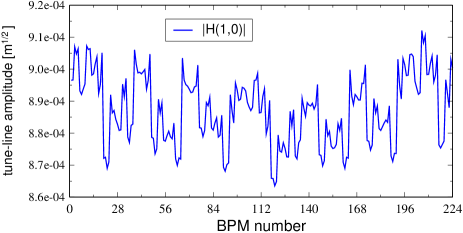
Refer to caption

Refer to caption

Figure 28: (Color) Example of variation of the horizontal (top) and vertical (bottom) tune-line amplitudes along the ESRF storage ring (224 BPMs, tracking simulations and FFT with initial conditions x0=8subscript𝑥08x_{0}=8 mm and y0=2.0subscript𝑦02.0y_{0}=2.0 mm, last row of table 16). Normal sextupoles induce a modulation in both planes of about 2%percent22\%, which would be zero in their absence.

Given a certain sextupole setting, THx,Hysubscript𝑇𝐻𝑥𝐻𝑦T_{Hx,Hy} and TVx,Vysubscript𝑇𝑉𝑥𝑉𝑦T_{Vx,Vy} are fixed. It is then of interest to estimate the largest beam oscillation amplitude that keeps the modulation below a tolerable level. To this end, preliminary single-particle tracking simulations at different initial conditions x0subscript𝑥0x_{0} and y0subscript𝑦0y_{0} (i.e. amplitudes) may be carried out. By storing the particle positions at all BPMs and performing the FFT of the Courant-Snyder coordinates x~~𝑥\tilde{x} and y~~𝑦\tilde{y}, the tune-line amplitudes may be plotted along the ring and their modulation evaluated against x0subscript𝑥0x_{0} and y0subscript𝑦0y_{0}. In Fig. 28 an example with betatron oscillations of x0=10subscript𝑥010x_{0}=10 mm and y0=2.2subscript𝑦02.2y_{0}=2.2 mm (large values by ESRF standards) is shown. Focusing errors are included in the model when computing the beta functions and the residual modulation of about 3%percent33\% is generated exclusively by sextupole RDTs. Results from a more complete scan of the ESRF storage ring are reported in Table 16. They suggest to limit the transverse oscillation to x03.5similar-to-or-equalssubscript𝑥03.5x_{0}\simeq 3.5 mm and y01similar-to-or-equalssubscript𝑦01y_{0}\simeq 1 mm, corresponding to 2Ix2Iy3.1×104similar-to-or-equals2subscript𝐼𝑥2subscript𝐼𝑦similar-to-or-equals3.1superscript104\sqrt{2I_{x}}\simeq\sqrt{2I_{y}}\simeq 3.1\times 10^{-4} m1/2 with relative variation of about 0.2%percent0.20.2\%, well within the measurement statistical fluctuations of about 1%percent11\%. Larger oscillations would induce a beneficial larger spectral resolution (higher ratio between sextupolar secondary lines and background noise), but also a larger modulation of the tune-line amplitudes, which is detrimental for the correct evaluation of the invariants 2Ix,y2subscript𝐼𝑥𝑦2I_{x,y}, hampering in turn the correct measurements of sextupolar RDTs.

Table 16: Dependence of tune-line amplitudes mean value and rms modulation against initial conditions evaluated from single-particle tracking and FFT of the particle position recorded at the 224 BPMs if the ESRF storage ring. The sextupole setting is the same used in the experiments and the focusing errors are included in the lattice model when computing the β𝛽\beta functions used to normalize x𝑥x and y𝑦y.
(x0,y0)subscript𝑥0subscript𝑦0(x_{0},y_{0}) (|H(1,0)|,|V(0,1)|)𝐻10𝑉01(|H(1,0)|,|V(0,1)|) (|H(1,0)|,|V(0,1)|)𝐻10𝑉01(|H(1,0)|,|V(0,1)|) rel.
mean value rms modul. modul.
(mm) m1/2 m1/2
(0.4, 0.1) (0.3, 0.3)×1040.30.3superscript104(0.3,\ 0.3)\times 10^{-4} (3.1, 2.7)×1093.12.7superscript109(3.1,\ 2.7)\times 10^{-9} 104similar-toabsentsuperscript104\sim 10^{-4}
(1.2, 0.5) (1.0, 1.4)×1041.01.4superscript104(1.0,\ 1.4)\times 10^{-4} (4.6, 5.0)×1084.65.0superscript108(4.6,\ 5.0)\times 10^{-8} <103absentsuperscript103<10^{-3}
(2.2, 0.5) (2.0, 1.4)×1042.01.4superscript104(2.0,\ 1.4)\times 10^{-4} (0.1, 0.1)×1060.10.1superscript106(0.1,\ 0.1)\times 10^{-6} <103absentsuperscript103<10^{-3}
(2.2, 0.7) (2.0, 2.0)×1042.02.0superscript104(2.0,\ 2.0)\times 10^{-4} (0.2, 0.2)×1060.20.2superscript106(0.2,\ 0.2)\times 10^{-6} 0.1%similar-toabsentpercent0.1\sim 0.1\%
(2.8, 0.8) (2.6, 2.6)×1042.62.6superscript104(2.6,\ 2.6)\times 10^{-4} (0.4, 0.4)×1060.40.4superscript106(0.4,\ 0.4)\times 10^{-6} 0.2%similar-toabsentpercent0.2\sim 0.2\%
(4.5, 0.8) (4.1, 2.6)×1044.12.6superscript104(4.1,\ 2.6)\times 10^{-4} (0.8, 0.9)×1060.80.9superscript106(0.8,\ 0.9)\times 10^{-6} 0.3%similar-toabsentpercent0.3\sim 0.3\%
(4.4, 0.9) (4.1, 3.0)×1044.13.0superscript104(4.1,\ 3.0)\times 10^{-4} (0.9, 1.1)×1060.91.1superscript106(0.9,\ 1.1)\times 10^{-6} 0.4%similar-toabsentpercent0.4\sim 0.4\%
(8.0, 2.0) (8.9, 6.9)×1048.96.9superscript104(8.9,\ 6.9)\times 10^{-4} (1.1, 1.5)×1051.11.5superscript105(1.1,\ 1.5)\times 10^{-5} 2%similar-toabsentpercent2\sim 2\%

As reported in Ref.Bartolini1 , the spectral line Hh(1,0)subscript𝐻10H_{h}(-1,0) of the complex C-S signals x~ip~x~𝑥𝑖subscript~𝑝𝑥\tilde{x}-i\tilde{p}_{x} receives a contribution from the normal octupole term x4superscript𝑥4x^{4} via two ORDTs, g3100subscript𝑔3100g_{3100} and g2011subscript𝑔2011g_{2011}. It can be shown that

Hh(1,0)subscript𝐻10\displaystyle H_{h}(-1,0) =\displaystyle= [3g3100(2Ix)3/2+4g2011(2Ix)1/2(2Iy)]×\displaystyle\left[3g_{3100}(2I_{x})^{3/2}+4g_{2011}(2I_{x})^{1/2}(2I_{y})\right]\times (168)
(2i)ei(2πQxN+ψx0).2𝑖superscript𝑒𝑖2𝜋subscript𝑄𝑥𝑁subscript𝜓𝑥0\displaystyle(-2i)e^{-i(2\pi Q_{x}N+\psi_{x0})}\ .

This implies that, on top of the focusing errors not included in the model and second-order normal sextupole terms, the tune line H(1,0)𝐻10H(1,0) of the real C-S signal x~~𝑥\tilde{x} receives a contribution from octupolar terms, since H(1,0)=1/2[Hh(1,0)+Hh(1,0)]𝐻1012delimited-[]subscript𝐻10subscript𝐻10H(1,0)=1/2[H_{h}(1,0)+H_{h}(-1,0)]. Three problems arise at large excitation amplitude and or with large octupolar components in the lattice: (i)𝑖(i) The tune phase is affected by octupolar terms and the linear lattice modelling discussed in Sec. IV.2 is corrupted; (ii)𝑖𝑖(ii) It is no longer possible to extract any linear combination of g3100subscript𝑔3100g_{3100} and g2011subscript𝑔2011g_{2011}, because of the different dependence on the action of the two terms, (2Ix)3/2proportional-toabsentsuperscript2subscript𝐼𝑥32\propto(2I_{x})^{3/2} and (2Ix)1/2(2Iy)proportional-toabsentsuperscript2subscript𝐼𝑥122subscript𝐼𝑦\propto(2I_{x})^{1/2}(2I_{y}) respectively; (iii)𝑖𝑖𝑖(iii) The tune line amplitude is no longer equal to (2Ix)1/2superscript2subscript𝐼𝑥12(2I_{x})^{1/2} and the computation of the other CRDTs from Tables 2 and 9 are affected by an intrinsic error. Equivalent considerations apply for the vertical tune line, affected by the y4superscript𝑦4y^{4} octupolar terms, g0013subscript𝑔0013g_{0013} and g1102subscript𝑔1102g_{1102}.

In conclusion, the turn-by-turn analysis of the nonlinear lattice model may be carried out and the formulas of Tables 2 and 2 applied provided that: (i𝑖i) an independent measurement of linear lattice errors, and hence of coupling and beta-beat RDTs, is performed prior the harmonic analysis; (ii𝑖𝑖ii) focusing errors are included when computing the C-S parameters to be used when evaluating the first-order RDTs of Table 3 and when normalizing the measured turn-by-turn data before performing the FFT, x~=x/βx~𝑥𝑥subscript𝛽𝑥\tilde{x}=x/\sqrt{\beta_{x}} and y~=y/βy~𝑦𝑦subscript𝛽𝑦\tilde{y}=y/\sqrt{\beta_{y}}; If a residual important modulation of the tune-line amplitudes along the ring is observed, the BPM beta functions may be further corrected by requiring that each tune-line amplitude be equal to the mean value (among all BPMs); (iii𝑖𝑖𝑖iii) the transverse beam excitation is conveniently chosen as a trade off between maximizing the spectral signal-to-noise ratio and minimizing the tune-line amplitude modulation induced by sextupoles and octupoles. This will result in tune lines having the same amplitude along the ring (|H(1,0)|2Ix/2similar-to-or-equals𝐻102subscript𝐼𝑥2|H(1,0)|\simeq\sqrt{2I_{x}}/2 and |V(0,1)|2Iy/2similar-to-or-equals𝑉012subscript𝐼𝑦2|V(0,1)|\simeq\sqrt{2I_{y}}/2), in zero beta-beat RDTs, and hence in the possibility of using first-order RDTs for the analysis of normal sextupole errors.

Appendix D Combined RDTs from single-BPM turn-by-turn data

In this Appendix formulas for the single-BPM combined RDTs (CRDTs) of Tables 2 and 9 are derived from the results of Appendix B. As discussed in Appendix C it is assumed that quadrupole errors are included in the computation of the C-S parameters, i.e. that the modulated beta functions are used in evaluating x~=x/βx~𝑥𝑥subscript𝛽𝑥\tilde{x}=x/\sqrt{\beta_{x}} and y~=y/βy~𝑦𝑦subscript𝛽𝑦\tilde{y}=y/\sqrt{\beta_{y}}, and that transverse oscillations are sufficiently small to neglect the interference of sextupole and octupole RDTs on the tune lines and to avoid amplitude-dependent detuning: This will ensure that the two sums in Eqs. (A) and (A) do not contain the secondary lines Hh(±1,0)subscript𝐻plus-or-minus10H_{h}(\pm 1,0) and Vh(0,±1)subscript𝑉0plus-or-minus1V_{h}(0,\pm 1). Results for the skew quadrupole CRDTs are presented for completeness, even though they are not considered suitable for a refined evaluation of betatron coupling (as mentioned in Appendix C). Equations (A) and (A) may be rewritten as

hx(N)=2Ixei(2πQxN+ψx0)subscript𝑥𝑁limit-from2subscript𝐼𝑥superscript𝑒𝑖2𝜋subscript𝑄𝑥𝑁subscript𝜓𝑥0\displaystyle h_{x}(N)=\sqrt{2I_{x}}e^{i(2\pi Q_{x}N+\psi_{x0})}\ - (169)
2ijklmjgjklm(2Ix)j+k12(2Iy)l+m2×\displaystyle\qquad\qquad 2i\sum_{jklm}{jg_{jklm}(2I_{x})^{\frac{j+k-1}{2}}(2I_{y})^{\frac{l+m}{2}}}\ \times
ei[(1j+k)(2πQxN+ψx0)+(ml)(2πQyN+ψy0)],superscript𝑒𝑖delimited-[]1𝑗𝑘2𝜋subscript𝑄𝑥𝑁subscript𝜓𝑥0𝑚𝑙2𝜋subscript𝑄𝑦𝑁subscript𝜓𝑦0\displaystyle\qquad\qquad e^{i[(1-j+k)(2\pi Q_{x}N+\psi_{x0})+(m-l)(2\pi Q_{y}N+\psi_{y0})]}\ ,

and, equivalently for the vertical plane,

hy(N)=2Iyei(2πQyN+ψy0)subscript𝑦𝑁limit-from2subscript𝐼𝑦superscript𝑒𝑖2𝜋subscript𝑄𝑦𝑁subscript𝜓𝑦0\displaystyle h_{y}(N)=\sqrt{2I_{y}}e^{i(2\pi Q_{y}N+\psi_{y0})}\ - (170)
2ijklmlgjklm(2Ix)j+k2(2Iy)l+m12×\displaystyle\qquad\qquad 2i\sum_{jklm}{lg_{jklm}(2I_{x})^{\frac{j+k}{2}}(2I_{y})^{\frac{l+m-1}{2}}}\times
ei[(kj)(2πQxN+ψx0)+(1l+m)(2πQyN+ψy0)].superscript𝑒𝑖delimited-[]𝑘𝑗2𝜋subscript𝑄𝑥𝑁subscript𝜓𝑥01𝑙𝑚2𝜋subscript𝑄𝑦𝑁subscript𝜓𝑦0\displaystyle\qquad\qquad e^{i[(k-j)(2\pi Q_{x}N+\psi_{x0})+(1-l+m)(2\pi Q_{y}N+\psi_{y0})]}\ \ .

gjklmsubscript𝑔𝑗𝑘𝑙𝑚g_{jklm} are the ORDT of Tables 13,  13 and 14, measurable at the location of a generic BPM. The four index are selected according to the type of the magnetic elements exciting the RDTs and obey to the the selection rules of Table 17. The real parts of the above expressions read

x~(N)~𝑥𝑁\displaystyle\tilde{x}(N) =\displaystyle= 2Ix2[ei(2πQxN+ψx0)+c.c]+\displaystyle\frac{\sqrt{2I_{x}}}{2}\left[e^{i(2\pi Q_{x}N+\psi_{x0})}+c.c\right]\ +
2jklmj(2Ix)j+k12(2Iy)l+m2×\displaystyle\hskip-14.22636pt2\sum_{jklm}{j(2I_{x})^{\frac{j+k-1}{2}}(2I_{y})^{\frac{l+m}{2}}}\ \times
{gjklmei[(1j+k)(2πQxN+ψx0)+(ml)(2πQyN+ψy0)]},subscript𝑔𝑗𝑘𝑙𝑚superscript𝑒𝑖delimited-[]1𝑗𝑘2𝜋subscript𝑄𝑥𝑁subscript𝜓𝑥0𝑚𝑙2𝜋subscript𝑄𝑦𝑁subscript𝜓𝑦0\displaystyle\hskip-14.22636pt\Im\left\{g_{jklm}e^{i[(1-j+k)(2\pi Q_{x}N+\psi_{x0})+(m-l)(2\pi Q_{y}N+\psi_{y0})]}\right\}\ ,
y~(N)~𝑦𝑁\displaystyle\tilde{y}(N) =\displaystyle= 2Iy2[ei(2πQyN+ψy0)+c.c]+\displaystyle\frac{\sqrt{2I_{y}}}{2}\left[e^{i(2\pi Q_{y}N+\psi_{y0})}+c.c\right]\ +
2jklml(2Ix)j+k2(2Iy)l+m12×\displaystyle\hskip-14.22636pt2\sum_{jklm}{l(2I_{x})^{\frac{j+k}{2}}(2I_{y})^{\frac{l+m-1}{2}}}\ \times
{gjklmei[(kj)(2πQxN+ψx0)+(1l+m)(2πQyN+ψy0)]}.subscript𝑔𝑗𝑘𝑙𝑚superscript𝑒𝑖delimited-[]𝑘𝑗2𝜋subscript𝑄𝑥𝑁subscript𝜓𝑥01𝑙𝑚2𝜋subscript𝑄𝑦𝑁subscript𝜓𝑦0\displaystyle\hskip-14.22636pt\Im\left\{g_{jklm}e^{i[(k-j)(2\pi Q_{x}N+\psi_{x0})+(1-l+m)(2\pi Q_{y}N+\psi_{y0})]}\right\}\ .

In deriving the above equations, the relation {iz}={z}𝑖𝑧𝑧\Re\{iz\}=-\Im\{z\}, valid for any complex number z𝑧z, is used. c.c.formulae-sequence𝑐𝑐c.c. stands for complex conjugate. The following relations then apply

{(2Ix)=(2|H(1,0)|)2ψx0=arg{H(1,0)},\displaystyle\left\{\begin{aligned} (2I_{x})&=&(2|H(1,0)|)^{2}\\ \psi_{x0}&=&\hbox{arg}\{H(1,0)\}\end{aligned}\right.\ , (173)
{(2Iy)=(2|V(0,1)|)2ψy0=arg{V(0,1)}.\displaystyle\left\{\begin{aligned} (2I_{y})&=&(2|V(0,1)|)^{2}\\ \psi_{y0}&=&\hbox{arg}\{V(0,1)\}\end{aligned}\right.\ . (174)
Table 17: Selection of index relative to the magnets.
multipole kind    magnetic term index relations
normal quadrupole x2superscript𝑥2x^{2} j+k=2m+l=0formulae-sequence𝑗𝑘2𝑚𝑙0j+k=2\quad m+l=0
normal quadrupole y2superscript𝑦2y^{2} j+k=0m+l=2formulae-sequence𝑗𝑘0𝑚𝑙2j+k=0\quad m+l=2
skew quadrupole xy𝑥𝑦xy j+k=1m+l=1formulae-sequence𝑗𝑘1𝑚𝑙1j+k=1\quad m+l=1
normal sextupole x3superscript𝑥3x^{3} j+k=3m+l=0formulae-sequence𝑗𝑘3𝑚𝑙0j+k=3\quad m+l=0
normal sextupole xy2𝑥superscript𝑦2xy^{2} j+k=1m+l=2formulae-sequence𝑗𝑘1𝑚𝑙2j+k=1\quad m+l=2
skew sextupole y3superscript𝑦3y^{3} j+k=0m+l=3formulae-sequence𝑗𝑘0𝑚𝑙3j+k=0\quad m+l=3
skew sextupole x2ysuperscript𝑥2𝑦x^{2}y j+k=2m+l=1formulae-sequence𝑗𝑘2𝑚𝑙1j+k=2\quad m+l=1
normal octupole x4superscript𝑥4x^{4} j+k=4m+l=0formulae-sequence𝑗𝑘4𝑚𝑙0j+k=4\quad m+l=0
normal octupole y4superscript𝑦4y^{4} j+k=0m+l=4formulae-sequence𝑗𝑘0𝑚𝑙4j+k=0\quad m+l=4
normal octupole x2y2superscript𝑥2superscript𝑦2x^{2}y^{2} j+k=2m+l=2formulae-sequence𝑗𝑘2𝑚𝑙2j+k=2\quad m+l=2

Coupling CRDTs. By replacing gjklmsubscript𝑔𝑗𝑘𝑙𝑚g_{jklm} with the first-order RDTs fjklm(1)superscriptsubscript𝑓𝑗𝑘𝑙𝑚1f_{jklm}^{(1)} and selecting in Eq. (D) those terms satisfying the conditions j+k=1𝑗𝑘1j+k=1 and m+l=1𝑚𝑙1m+l=1 the following harmonics are generated

22Iy{f1001(1)ei(2πQyN+ψy0)]+f1010(1)ei(2πQyN+ψy0)]}=\displaystyle 2\sqrt{2I_{y}}\Im\left\{f_{1001}^{(1)}e^{i(2\pi Q_{y}N+\psi_{y0})]}+f_{1010}^{(1)}e^{-i(2\pi Q_{y}N+\psi_{y0})]}\right\}= (175)
2Iyi[(f1001(1)f1010(1))ei(2πQyN+ψy0)\displaystyle\frac{\sqrt{2I_{y}}}{i}\left[\left(f_{1001}^{(1)}-f_{1010}^{(1)*}\right)e^{i(2\pi Q_{y}N+\psi_{y0})}-\right.
(f1001(1)f1010(1))ei(2πQyN+ψy0)]=\displaystyle\hskip 31.2982pt\left.\left(f_{1001}^{(1)*}-f_{1010}^{(1)}\right)e^{-i(2\pi Q_{y}N+\psi_{y0})}\right]=
2Iyi[Fxyei(2πQyN+ψy0)c.c.],\displaystyle\frac{\sqrt{2I_{y}}}{i}\left[F_{xy}e^{i(2\pi Q_{y}N+\psi_{y0})}-c.c.\right]\ ,

where the coupling CRDT is defined as Fxy=f1001(1)f1010(1)subscript𝐹𝑥𝑦superscriptsubscript𝑓10011superscriptsubscript𝑓10101F_{xy}=f_{1001}^{(1)}-f_{1010}^{(1)*} and excites the spectral line is H(0,1)𝐻01H(0,1), whose amplitude and phase are then

{|H(0,1)|=2Iy|Fxy|arg{H(0,1)}=qFxy+32π+ψy0.\displaystyle\left\{\begin{aligned} |H(0,1)|&=\sqrt{2I_{y}}|F_{xy}|\\ \hbox{arg}\{H(0,1)\}&=q_{F_{xy}}+\frac{3}{2}\pi+\psi_{y0}\end{aligned}\right.\ . (176)

(2Iy)2subscript𝐼𝑦(2I_{y}) and ψy0subscript𝜓𝑦0\psi_{y0} are measurable from the vertical tune line V(0,1)𝑉01V(0,1), via Eq. (174), yielding

{Fxy=f1001(1)f1010(1)|Fxy|=|H(0,1)|/(2|V(0,1)|)qFxy=arg{H(0,1)}32πarg{V(0,1)}.\displaystyle\left\{\begin{aligned} F_{xy}&=f_{1001}^{(1)}-f_{1010}^{(1)*}\\ |F_{xy}|&=|H(0,1)|/(2|V(0,1)|)\\ q_{F_{xy}}&=\hbox{arg}\{H(0,1)\}-\frac{3}{2}\pi-\hbox{arg}\{V(0,1)\}\end{aligned}\right.\ .\hskip 28.45274pt (177)

The same algebra repeated for the vertical signal of Eq. (D) reads

22Ix{f0110(1)ei(2πQxN+ψx0)]+f1010(1)ei(2πQxN+ψx0)]}=\displaystyle 2\sqrt{2I_{x}}\Im\left\{f_{0110}^{(1)}e^{i(2\pi Q_{x}N+\psi_{x0})]}+f_{1010}^{(1)}e^{-i(2\pi Q_{x}N+\psi_{x0})]}\right\}=
2Ixi[(f0110(1)f1010(1))ei(2πQxN+ψx0)\displaystyle\frac{\sqrt{2I_{x}}}{i}\left[\left(f_{0110}^{(1)}-f_{1010}^{(1)*}\right)e^{i(2\pi Q_{x}N+\psi_{x0})}-\right.
(f0110(1)f1010(1))ei(2πQxN+ψx0)]=\displaystyle\hskip 31.2982pt\left.\left(f_{0110}^{(1)*}-f_{1010}^{(1)}\right)e^{-i(2\pi Q_{x}N+\psi_{x0})}\right]=
2Ixi[Fyxei(2πQxN+ψx0)c.c.],\displaystyle\frac{\sqrt{2I_{x}}}{i}\left[F_{yx}e^{i(2\pi Q_{x}N+\psi_{x0})}-c.c.\right]\ , (178)

where the coupling CRDT is defined as Fyx=f0110(1)f1010(1)subscript𝐹𝑦𝑥superscriptsubscript𝑓01101superscriptsubscript𝑓10101F_{yx}=f_{0110}^{(1)}-f_{1010}^{(1)*} and excites the spectral line is V(1,0)𝑉10V(1,0), whose amplitude and phase are then

{|V(1,0)|=2Ix|Fyx|arg{V(1,0)}=qFyx+32π+ψx0.\displaystyle\left\{\begin{aligned} |V(1,0)|&=\sqrt{2I_{x}}|F_{yx}|\\ \hbox{arg}\{V(1,0)\}&=q_{F_{yx}}+\frac{3}{2}\pi+\psi_{x0}\end{aligned}\right.\ . (179)

(2Ix)2subscript𝐼𝑥(2I_{x}) and ψx0subscript𝜓𝑥0\psi_{x0} are measurable from the horizontal tune line H(1,0)𝐻10H(1,0), via Eq. (173), yielding

{Fyx=f0110(1)f1010(1)|Fyx|=|V(1,0)|/(2|H(1,0)|)qFyx=arg{V(1,0)}32πarg{H(1,0)}.\displaystyle\left\{\begin{aligned} F_{yx}&=f_{0110}^{(1)}-f_{1010}^{(1)*}\\ |F_{yx}|&=|V(1,0)|/(2|H(1,0)|)\\ q_{F_{yx}}&=\hbox{arg}\{V(1,0)\}-\frac{3}{2}\pi-\hbox{arg}\{H(1,0)\}\end{aligned}\right.\ .\hskip 28.45274pt (180)

Equations (177) and (180) prove the skew quadrupole entries in Tables 2 and  2. Interestingly, one may think of inverting the linear system

{Fxy=f1001(1)f1010(1)Fyx=f1001(1)f1010(1),\displaystyle\left\{\begin{aligned} F_{xy}&=f_{1001}^{(1)}-f_{1010}^{(1)*}\\ F_{yx}&=f_{1001}^{(1)*}-f_{1010}^{(1)*}\\ \end{aligned}\right.\ ,\hskip 28.45274pt (181)

to extract the coupling RDTs from the two CRDTs. Unfortunately, the system is degenerate and this is not possible. Nevertheless, the following relation applies

Fxy0={Fxy}{Fyx}0.subscript𝐹𝑥𝑦0subscript𝐹𝑥𝑦subscript𝐹𝑦𝑥0\displaystyle F_{xy0}=\Re\{F_{xy}\}-\Re\{F_{yx}\}\equiv 0\ . (182)

Fxy0subscript𝐹𝑥𝑦0F_{xy0} may be then used to asses the reliability of the harmonic analysis, as far as coupling is concerned, in the same way F0subscript𝐹0F_{0} of Eq. (7) does it for the sextupolar analysis.

Normal sextupole CRDTs. Normal sextupoles excite several spectral lines. As for the coupling case, ORDTs gjklmsubscript𝑔𝑗𝑘𝑙𝑚g_{jklm} are replaced by first-order RDTs fjklm(1)superscriptsubscript𝑓𝑗𝑘𝑙𝑚1f_{jklm}^{(1)}. The potential term proportional to x3superscript𝑥3x^{3} excites the lines H(±2,0)𝐻plus-or-minus20H(\pm 2,0) and H(0,0)𝐻00H(0,0). The latter represents an offset and is not considered an Observable, as it contains dispersive terms, BPM offsets and contributions from other RDTs. By making use of Eq. (129) and selecting in Eq. (D) the RDTs exciting H(±2,0)𝐻plus-or-minus20H(\pm 2,0), the following harmonics are generated

4Ix{3f3000(1)e2i(2πQxN+ψx0)]+f1200(1)e2i(2πQxN+ψx0)]}=\displaystyle 4I_{x}\Im\left\{3f_{3000}^{(1)}e^{-2i(2\pi Q_{x}N+\psi_{x0})]}+f_{1200}^{(1)}e^{2i(2\pi Q_{x}N+\psi_{x0})]}\right\}=
(2Ix)i[(3f3000(1)f1200(1))e2i(2πQxN+ψx0)\displaystyle\frac{(2I_{x})}{i}\left[\left(3f_{3000}^{(1)}-f_{1200}^{(1)*}\right)e^{-2i(2\pi Q_{x}N+\psi_{x0})}-\right.
(3f3000(1)f1200(1))e2i(2πQxN+ψx0)]=\displaystyle\hskip 31.2982pt\left.\left(3f_{3000}^{(1)*}-f_{1200}^{(1)}\right)e^{2i(2\pi Q_{x}N+\psi_{x0})}\right]=
(2Ix)i[FNS3e2i(2πQxN+ψx0)c.c.],\displaystyle\frac{(2I_{x})}{i}\left[F_{NS3}e^{-2i(2\pi Q_{x}N+\psi_{x0})}-c.c.\right]\ , (183)

where the corresponding sextupolar CRDT is defined as FNS3=3f3000(1)f1200(1)subscript𝐹𝑁𝑆33superscriptsubscript𝑓30001superscriptsubscript𝑓12001F_{NS3}=3f_{3000}^{(1)}-f_{1200}^{(1)*} and excites the spectral line is H(2,0)𝐻20H(-2,0), whose amplitude and phase are then

{|H(2,0)|=(2Ix)|FNS3|arg{H(2,0)}=qFNS3+32π2ψx0.\displaystyle\left\{\begin{aligned} |H(-2,0)|&=(2I_{x})|F_{NS3}|\\ \hbox{arg}\{H(-2,0)\}&=q_{F_{NS3}}+\frac{3}{2}\pi-2\psi_{x0}\end{aligned}\right.\ . (184)

As for the coupling case, the tune line is used to extract amplitude and phase of FNS3subscript𝐹𝑁𝑆3F_{NS3}:

{FNS3=3f3000(1)f1200(1)|FNS3|=|H(2,0)|/(4|H(1,0)|2)qFNS3=arg{H(2,0)}32π+2arg{H(1,0)}.\displaystyle\left\{\begin{aligned} F_{NS3}&=3f_{3000}^{(1)}-f_{1200}^{(1)*}\\ |F_{NS3}|&=|H(-2,0)|/(4|H(1,0)|^{2})\\ q_{F_{NS3}}&=\hbox{arg}\{H(-2,0)\}-\frac{3}{2}\pi+2\hbox{arg}\{H(1,0)\}\end{aligned}\right..\hskip 28.45274pt (185)

The mixing potential term proportional to xy2𝑥superscript𝑦2xy^{2} excite several lines: H(0,±2)𝐻0plus-or-minus2H(0,\pm 2) in the horizontal spectrum, V(±1,±1)𝑉plus-or-minus1plus-or-minus1V(\pm 1,\pm 1) and V(±1,1)𝑉plus-or-minus1minus-or-plus1V(\pm 1,\mp 1) in the vertical. By repeating the same algebra in the sums of Eqs. (D) and (D) the following relations are derived:

{FNS2=f1020(1)f0120(1)|FNS2|=|H(0,2)|/(4|V(0,1)|2)qFNS2=arg{H(0,2)}32π+2arg{V(0,1)},\displaystyle\left\{\begin{aligned} F_{NS2}&=f_{1020}^{(1)}-f_{0120}^{(1)}\\ |F_{NS2}|&=|H(0,-2)|/(4|V(0,1)|^{2})\\ q_{F_{NS2}}&=\hbox{arg}\{H(0,-2)\}-\frac{3}{2}\pi+2\hbox{arg}\{V(0,1)\}\end{aligned}\right.,\hskip 28.45274pt (186)
{FNS1=2f1020(1)f0111(1)|FNS1|=|V(1,1)|/(4|H(1,0)||V(0,1)|)qFNS1=arg{V(1,1)}32π+arg{H(1,0)}+arg{V(0,1)},\displaystyle\left\{\begin{aligned} F_{NS1}&=2f_{1020}^{(1)}-f_{0111}^{(1)*}\\ |F_{NS1}|&=|V(-1,-1)|/(4|H(1,0)||V(0,1)|)\\ q_{F_{NS1}}&=\hbox{arg}\{V(-1,-1)\}-\frac{3}{2}\pi\ +\\ &\hskip 14.22636pt\hbox{arg}\{H(1,0)\}+\hbox{arg}\{V(0,1)\}\end{aligned}\right.,\hskip 45.52458pt (187)
{FNS0=2f0120(1)f0111(1)|FNS0|=|V(1,1)|/(4|H(1,0)||V(0,1)|)qFNS0=arg{V(1,1)}32πarg{H(1,0)}+arg{V(0,1)}.\displaystyle\left\{\begin{aligned} F_{NS0}&=2f_{0120}^{(1)*}-f_{0111}^{(1)}\\ |F_{NS0}|&=|V(1,-1)|/(4|H(1,0)||V(0,1)|)\\ q_{F_{NS0}}&=\hbox{arg}\{V(1,-1)\}-\frac{3}{2}\pi\ -\\ &\hskip 14.22636pt\hbox{arg}\{H(1,0)\}+\hbox{arg}\{V(0,1)\}\end{aligned}\right..\hskip 54.06006pt (188)

It is worthwhile noticing that the choice has been made here to select those lines laying within 0 and 0.5 in tune units, starting from betatron tunes of the ESRF storage ring, whose fractional parts are Qx=0.44subscript𝑄𝑥0.44Q_{x}=0.44 and Qy=0.39subscript𝑄𝑦0.39Q_{y}=0.39: H(2,0)𝐻20H(-2,0) appears at 12Qx=0.1212subscript𝑄𝑥0.121-2Q_{x}=0.12, H(0,2)𝐻02H(0,-2) at 12Qy=0.2212subscript𝑄𝑦0.221-2Q_{y}=0.22, V(1,1V(-1,-1) at 1QxQy=0.171subscript𝑄𝑥subscript𝑄𝑦0.171-Q_{x}-Q_{y}=0.17 and V(1,1)𝑉11V(1,-1) at QxQy=0.05subscript𝑄𝑥subscript𝑄𝑦0.05Q_{x}-Q_{y}=0.05. This choice is however arbitrary. Their complex conjugates may be used as well, V(1,1)𝑉11V(-1,1) instead of V(1,1)𝑉11V(1,-1) for instance, on condition to modify accordingly the computation of the CRDT phase.

Skew sextupole CRDTs. The potential term proportional to y3superscript𝑦3y^{3} excites the lines V(0,±2)𝑉0plus-or-minus2V(0,\pm 2) and V(0,0)𝑉00V(0,0) (not used). After selecting the RDTs in Eq. (D) exciting these lines and repeating the same algebra carried out for the normal sextupole, the following harmonics are generated

4Iy{3g0030e2i(2πQyN+ψy0)]+g0012e2i(2πQyN+ψy0)]}=\displaystyle 4I_{y}\Im\left\{3g_{0030}e^{-2i(2\pi Q_{y}N+\psi_{y0})]}+g_{0012}e^{2i(2\pi Q_{y}N+\psi_{y0})]}\right\}=
(2Iy)i[(3g0030g0012)e2i(2πQyN+ψy0)\displaystyle\frac{(2I_{y})}{i}\left[\left(3g_{0030}-g_{0012}^{*}\right)e^{-2i(2\pi Q_{y}N+\psi_{y0})}-\right.
(3g0030g0012)e2i(2πQyN+ψy0)]=\displaystyle\hskip 31.2982pt\left.\left(3g_{0030}^{*}-g_{0012}\right)e^{2i(2\pi Q_{y}N+\psi_{y0})}\right]=
(2Iy)i[FSS3e2i(2πQyN+ψy0)c.c.].\displaystyle\frac{(2I_{y})}{i}\left[F_{SS3}e^{-2i(2\pi Q_{y}N+\psi_{y0})}-c.c.\right]\ . (189)

The corresponding skew sextupolar CRDT reads FSS3=3g0030g0012subscript𝐹𝑆𝑆33superscriptsubscript𝑔0030superscriptsubscript𝑔0012F_{SS3}=3g_{0030}^{*}-g_{0012}^{*}. FSS3subscript𝐹𝑆𝑆3F_{SS3} excites the spectral line V(0,2)𝑉02V(0,-2), whose amplitude and phase are then

{|V(0,2)|=(2Iy)|FSS3|arg{V(0,2)}=qFSS3+32π2ψy0,\displaystyle\left\{\begin{aligned} |V(0,-2)|&=(2I_{y})|F_{SS3}|\\ \hbox{arg}\{V(0,-2)\}&=q_{F_{SS3}}+\frac{3}{2}\pi-2\psi_{y0}\end{aligned}\right.\ , (190)

yielding

{FSS3=3g3000g1200|FSS3|=|V(0,2)|/(4|V(1,0)|2)qFSS3=arg{V(0,2)}32π+2arg{V(0,1)}.\displaystyle\left\{\begin{aligned} F_{SS3}&=3g_{3000}-g_{1200}^{*}\\ |F_{SS3}|&=|V(0,-2)|/(4|V(1,0)|^{2})\\ q_{F_{SS3}}&=\hbox{arg}\{V(0,-2)\}-\frac{3}{2}\pi+2\hbox{arg}\{V(0,1)\}\end{aligned}\right..\hskip 28.45274pt (191)

The mixing potential term proportional to x2ysuperscript𝑥2𝑦x^{2}y excites several lines: V(±2,0)𝑉plus-or-minus20V(\pm 2,0) in the vertical spectrum, H(±1,±1)𝐻plus-or-minus1plus-or-minus1H(\pm 1,\pm 1) and H(±1,1)𝐻plus-or-minus1minus-or-plus1H(\pm 1,\mp 1) in the horizontal one. By repeating the same algebra in the sums of Eqs. (D) and (D), the following relations are derived:

{FSS2=g2010,Vg0210|FSS2|=|V(2,0)|/(4|H(1,0)|2)qFSS2=arg{V(2,0)}32π+2arg{H(1,0)},\displaystyle\left\{\begin{aligned} F_{SS2}&=g_{2010,V}^{*}-g_{0210}^{*}\\ |F_{SS2}|&=|V(-2,0)|/(4|H(1,0)|^{2})\\ q_{F_{SS2}}&=\hbox{arg}\{V(-2,0)\}-\frac{3}{2}\pi+2\hbox{arg}\{H(1,0)\}\end{aligned}\right.,\hskip 28.45274pt (192)
{FSS1=2g2010,Hg1101|FSS1|=|H(1,1)|/(4|H(1,0)||V(0,1)|)qFSS1=arg{H(1,1)}32π+arg{H(1,0)}+arg{V(0,1)},\displaystyle\left\{\begin{aligned} F_{SS1}&=2g_{2010,H}-g_{1101}^{*}\\ |F_{SS1}|&=|H(-1,-1)|/(4|H(1,0)||V(0,1)|)\\ q_{F_{SS1}}&=\hbox{arg}\{H(-1,-1)\}-\frac{3}{2}\pi\ +\\ &\hskip 14.22636pt\hbox{arg}\{H(1,0)\}+\hbox{arg}\{V(0,1)\}\end{aligned}\right.,\hskip 45.52458pt (193)
{FSS0=g11102g2001|FSS0|=|H(1,1)|/(4|H(1,0)||V(0,1)|)qFSS0=arg{H(1,1)}32πarg{H(1,0)}+arg{V(0,1)}.\displaystyle\left\{\begin{aligned} F_{SS0}&=g_{1110}-2g_{2001}^{*}\\ |F_{SS0}|&=|H(1,-1)|/(4|H(1,0)||V(0,1)|)\\ q_{F_{SS0}}&=\hbox{arg}\{H(1,-1)\}-\frac{3}{2}\pi\ -\\ &\hskip 14.22636pt\hbox{arg}\{H(1,0)\}+\hbox{arg}\{V(0,1)\}\end{aligned}\right..\hskip 54.06006pt (194)

Normal octupole CRDTs. In Table 15 Ref. Bartolini1 the list of spectral lines of the complex C-S signals x~ip~x~𝑥𝑖subscript~𝑝𝑥\tilde{x}-i\tilde{p}_{x} (y~ip~y~𝑦𝑖subscript~𝑝𝑦\tilde{y}-i\tilde{p}_{y}) excited by normal octupole terms (x4+y46x2y2)superscript𝑥4superscript𝑦46superscript𝑥2superscript𝑦2(x^{4}+y^{4}-6x^{2}y^{2}) is provided. The catalog is not complete, as two lines are missing, of which more later (the complete list may be found in Ref.Bartolini1 , though two terms f1120subscript𝑓1120f_{1120} and f1102subscript𝑓1102f_{1102} are mistakenly swapped). As far as the potential term x4superscript𝑥4x^{4} is concerned the lines H(±3,0)𝐻plus-or-minus30H(\pm 3,0) are excited. By making use of Eq. (129) and selecting in Eq. (D) the RDTs exciting this line, the following harmonics are generated

2(2Ix)3/2×\displaystyle 2(2I_{x})^{3/2}\times
{4g4000e3i(2πQxN+ψx0)]+g1300e3i(2πQxN+ψx0)]}=\displaystyle\Im\left\{4g_{4000}e^{-3i(2\pi Q_{x}N+\psi_{x0})]}+g_{1300}e^{3i(2\pi Q_{x}N+\psi_{x0})]}\right\}=
(2Ix)3/2i[(4g4000g1300)e3i(2πQxN+ψx0)\displaystyle\frac{(2I_{x})^{3/2}}{i}\left[\left(4g_{4000}-g_{1300}^{*}\right)e^{-3i(2\pi Q_{x}N+\psi_{x0})}-\right.
(4g4000g1300)e3i(2πQxN+ψx0)]=\displaystyle\hskip 31.2982pt\left.\left(4g_{4000}^{*}-g_{1300}\right)e^{3i(2\pi Q_{x}N+\psi_{x0})}\right]=
(2Ix)3/2i[FNO3e3i(2πQxN+ψx0)c.c.],\displaystyle\frac{(2I_{x})^{3/2}}{i}\left[-F_{NO3}e^{3i(2\pi Q_{x}N+\psi_{x0})}-c.c.\right]\ , (195)

where the CRDT is defined as FNO3=4g4000g1300subscript𝐹𝑁𝑂34superscriptsubscript𝑔4000subscript𝑔1300F_{NO3}=4g_{4000}^{*}-g_{1300} and excites the spectral line is H(3,0)𝐻30H(3,0), whose amplitude and phase are then

{|H(3,0)|=(2Ix)3/2|FNO3|arg{H(3,0)}=qFNO3+π2+3ψx0,\displaystyle\left\{\begin{aligned} |H(3,0)|&=(2I_{x})^{3/2}|F_{NO3}|\\ \hbox{arg}\{H(3,0)\}&=q_{F_{NO3}}+\frac{\pi}{2}+3\psi_{x0}\end{aligned}\right.\ , (196)

and

{FNO3=4g4000g1300|FNO3|=|H(3,0)|/(8|H(1,0)|3)qFNO3=arg{H(3,0)}π23arg{H(1,0)}.\displaystyle\left\{\begin{aligned} F_{NO3}&=4g_{4000}^{*}-g_{1300}\\ |F_{NO3}|&=|H(3,0)|/(8|H(1,0)|^{3})\\ q_{F_{NO3}}&=\hbox{arg}\{H(3,0)\}-\frac{\pi}{2}-3\hbox{arg}\{H(1,0)\}\end{aligned}\right..\hskip 28.45274pt (197)

the spectral line H(3,0)𝐻30H(3,0) of the real C-S signal x~~𝑥\tilde{x} is used because for the ESRF tune working point this is the one laying within 0 and 0.5 . The vertical potential term y4superscript𝑦4y^{4} excites the vertical lines V(0,±3)𝑉0plus-or-minus3V(0,\pm 3), resulting in

{FNO5=4g0040g0013|FNO5|=|V(0,3)|/(8|V(0,1)|3)qFNO5=arg{V(0,3)}π23arg{V(0,1)}.\displaystyle\left\{\begin{aligned} F_{NO5}&=4g_{0040}^{*}-g_{0013}\\ |F_{NO5}|&=|V(0,3)|/(8|V(0,1)|^{3})\\ q_{F_{NO5}}&=\hbox{arg}\{V(0,3)\}-\frac{\pi}{2}-3\hbox{arg}\{V(0,1)\}\end{aligned}\right..\hskip 28.45274pt (198)

As far as the mixing potential term x2y2superscript𝑥2superscript𝑦2x^{2}y^{2} is concerned, the lines H(±1,2)𝐻plus-or-minus12H(\pm 1,2) and V(2,±1)𝑉2plus-or-minus1V(2,\pm 1) are generated by four CRDTs:

{FNO4=2g2020,Hg1102|FNO4|=|H(1,2)|/(8|H(1,0)||V(0,1)|2)qFNO4=arg{H(1,2)}π2arg{H(1,0)}2arg{V(0,1)},\displaystyle\left\{\begin{aligned} F_{NO4}&=2g_{2020,H}^{*}-g_{1102}\\ |F_{NO4}|&=|H(1,2)|/(8|H(1,0)||V(0,1)|^{2})\\ q_{F_{NO4}}&=\hbox{arg}\{H(1,2)\}-\frac{\pi}{2}\\ &\hskip 14.22636pt-\hbox{arg}\{H(1,0)\}-2\hbox{arg}\{V(0,1)\}\end{aligned}\right.,\hskip 28.45274pt (199)
{FNO2=2g2002g1120|FNO2|=|H(1,2)|/(8|H(1,0)||V(0,1)|2)qFNO2=arg{H(1,2)}+π2+arg{H(1,0)}2arg{V(0,1)},\displaystyle\left\{\begin{aligned} F_{NO2}&=2g_{2002}-g_{1120}^{*}\\ |F_{NO2}|&=|H(-1,2)|/(8|H(1,0)||V(0,1)|^{2})\\ q_{F_{NO2}}&=\hbox{arg}\{H(-1,2)\}+\frac{\pi}{2}\\ &\hskip 14.22636pt+\hbox{arg}\{H(1,0)\}-2\hbox{arg}\{V(0,1)\}\end{aligned}\right.,\hskip 28.45274pt (200)
{FNO1=2g0220g2011|FNO1|=|V(2,1)|/(8|H(1,0)|2|V(0,1)|)qFNO1=arg{V(2,1)}+π22arg{H(1,0)}+arg{V(0,1)},\displaystyle\left\{\begin{aligned} F_{NO1}&=2g_{0220}-g_{2011}^{*}\\ |F_{NO1}|&=|V(2,-1)|/(8|H(1,0)|^{2}|V(0,1)|)\\ q_{F_{NO1}}&=\hbox{arg}\{V(2,-1)\}+\frac{\pi}{2}\\ &\hskip 14.22636pt-2\hbox{arg}\{H(1,0)\}+\hbox{arg}\{V(0,1)\}\end{aligned}\right.,\hskip 28.45274pt (201)
{FNO0=2g2020,Vg0211|FNO0|=|V(2,1)|/(8|H(1,0)|2|V(0,1)|)qFNO0=arg{V(2,1)}π22arg{H(1,0)}arg{V(0,1)}.\displaystyle\left\{\begin{aligned} F_{NO0}&=2g_{2020,V}^{*}-g_{0211}\\ |F_{NO0}|&=|V(2,1)|/(8|H(1,0)|^{2}|V(0,1)|)\\ q_{F_{NO0}}&=\hbox{arg}\{V(2,1)\}-\frac{\pi}{2}\\ &\hskip 14.22636pt-2\hbox{arg}\{H(1,0)\}-\hbox{arg}\{V(0,1)\}\end{aligned}\right..\hskip 28.45274pt (202)

References

  • (1) D.D. Caussyn, M. Ball, B. Brabson, J. Collins, S.A. Crtis, V. Derenchuk, D. Duplantis, G. East, M. Ellison, T. ellison, D. Friesel, B. Hamilton, W.P. jones, W. Lamble, S.Y. lee, D. Li, M.G. Minty, T. Sloan, G. Xu, A.W. Chao, K.Y. Ng, S. Tepikian, Experimental Studies of Nonlinear Beam Dynamics, Phys. Rev. A 46, 7942 (1992).
  • (2) A. Bazzani, E. Todesco, G. Turchetti, G. Servizi, A Normal Form Approach to the Theory of the Nonlinear Betatronic Motion, CERN 94-02 (1994).
  • (3) É. Forest et al., Normal Form Methods for Complicated Periodic Systems: a Comlpete Solution using Differential Algebra, Particle Accelerators, vol. 24 (1989), pp. 91-113.
  • (4) R. Bartolini and F. Schmidt, Normal Form via Tracking or Beam Data, LHC Project note 132 (revised 3rdsuperscript3𝑟𝑑3^{rd} revision May 2005), Part. Accelerators. 59, pp. 93–106, (1998).
  • (5) R. Tomás García, Direct Measurement of Resonance Driving Terms in the Super Proton Synchrotron (SPS) of CERN using Beam Position Monitors, PhD thesis, CERN-THESIS-2003-010 (2003).
  • (6) A. Franchi, Studies and Measurements of Linear Coupling and Nonlinearities in Hadron Circular Accelerators, PhD thesis, GSI DISS 2006-07 (2006).
  • (7) A. Franchi, R. Tomás García and F. Schmidt, Magnet Strength Measurement in Circular Accelerators from Beam Position Monitor Data, Phys. Rev. ST Accel. Beams vol. 10, 074001 (2007)
  • (8) J. S. Kolski, R. J. Macek, R. C. McCrady, and X. Pang, Independent component analysis applied to long bunch beams in the Los Alamos Proton Storage Ring, Phys. Rev. ST Accel. Beams, vol. 15, 112802 (2012); X. Pang and S.Y. Lee, Independent component analysis for beam measurements , J. Appl. Phys. vol. 106, 074902 (2009); X. Pang, Ph.D. thesis, Indiana University, 2009.
  • (9) R. Bartolini, I. P. S. Martin, J. H. Rowland, P. Kuske and F. Schmidt, Correction of multiple nonlinear resonances in storage rings, Phys. Rev. ST Accel. Beams, vol. 11, 104002 (2008);
  • (10) T. Bach, S. Gilardoni, M. Giovannozzi, C. Hernalsteens, A. Lachaize, G. Sterbini, R. Tomás and R. Wasef, CERN PS optical properties measured with turn-by-turn orbit data, Proceedings of IPAC2013, p 2627, Shanghai, China (2009).
  • (11) J. Laskar, C. Froeschlé and A. Celletti, The Measure of Chaos by the Numerical Analysis of the Fundamental Frequencies. Application to the Standard Mapping, Physica D 56, 253-269 (1992).
  • (12) R.Bartolini, A. Bazzani, M. Giovannozzi, W. Scandale and E. Todesco, Tune evaluation in simulations and experiments CERN SL/95-84 (AP) (1995).
  • (13) N. Minty and F. Zimmermann, Measurement and Control of Charged Particle Beams, Springer, Berlin, 2003 (ISBN 3-540-44197-5).
  • (14) R. E. Meller, A. W. Chao, J. M. Pereson, S. G. Peggs and M. Furman, Decoherence of kicked beamsm SSC-N-360, 1987.
  • (15) B. K. Scheidt and F. Epaud, Installation and Commissioning of a Complete Upgrade of the BPM System for the ESRF Storage ring, Proceedings of DIPAC09, p 50, Basel, Switzerland, (2009).
  • (16) A. Kosicek Modified Digital Filtering Makes Possible True and Pure Turn-by-Turn Measurements, Proceedings of BIW08, p 186, Lake Tahoe, USA (2008).
  • (17) W. Herr, F. Schmidt A MAD-X Primer, CERN AB Note, CERN-AB-2004-027-ABP (2004)
  • (18) R. Tomás, Normal form of particle motion under the influence of an AC dipole, Phys. Rev. ST Accel. Beams vol. 5, 054001 (2002).
  • (19) S. White, E. Maclean and R. Tomás, Direct amplitude detuning measurement with ac dipole, Phys. Rev. ST Accel. Beams, vol. 16, 071002 (2013).
  • (20) D. Martin, Results of SR SY Surveys October SD 2013, ESRF survey note ESRF-TS-ALGE/1722DM (2013).
  • (21) J. Jacob, Y. Papaphilippou and A.Ropert, Parameter List of the ESRF Accelerator Complex, ESRF note ESRF/MACH 04/60 (2004).
  • (22) J. Bengtsson and J. Irwin, Analytical calculation of smear and tune shift, SSC Note, SSC-232, Berkeley, CA, (1990)
  • (23) A. Franchi, S. Gilardoni and M. Giovannozzi, Progresses in the studies of adiabatic splitting of charged particle beams by crossing nonlinear resonances, Phys. Rev. ST Accel. Beams, vol. 12, 014001 (2009).
  • (24) R. Tomás, M. Bai, R. Calaga, W. Fischer, A. Franchi and G. Rumolo, “Measurement of global and local resonance terms”, Phys. Rev. ST Accel. Beams 8, issue 2, 024001 (2005).
  • (25) P. Castro García, , Luminosity and beta function measurement at the electron-positron collider ring LEP, PhD thesis, CERN-SL-96-070-BI (1996).
  • (26) A. Franchi, E. Métral, and R. Tomás García, Emittance sharing and exchange driven by linear betatron coupling in circular accelerators, Phys. Rev. ST Accel. Beams, vol. 10, 064003 (2007).
  • (27) J. Safranek, Experimental determination of Storage Ring Optics Using Orbit Response Measurements, Nucl. Instr. and Meth. A, vol. 388, pp. 27-36 (1996).
  • (28) A. Franchi, L. Farvacque, J. Chavanne, F. Ewald, B. Nash, K. Scheidt and R. Tomás, Vertical emittance reduction and preservation in electron storage rings via resonance driving terms correction, Phys. Rev. ST Accel. Beams, vol. 14, 034002, (2011),
  • (29) G. Vanbavinckhove, M. Aiba, A. Nadji, L. Nadolski , R.Tomás, and M-A. Tordeux, Linear and non-linear optics measurements at SOLEIL, Proceedings of PAC09, p 3877, Vancouver, BC, Canada, 2009.