Feasibility-Seeking and Superiorization Algorithms Applied to Inverse Treatment Planning in Radiation Therapy

Abstract.

We apply the recently proposed superiorization methodology (SM) to the inverse planning problem in radiation therapy. The inverse planning problem is represented here as a constrained minimization problem of the total variation (TV) of the intensity vector over a large system of linear two-sided inequalities. The SM can be viewed conceptually as lying between feasibility-seeking for the constraints and full-fledged constrained minimization of the objective function subject to these constraints. It is based on the discovery that many feasibility-seeking algorithms (of the projection methods variety) are perturbation-resilient, and can be proactively steered toward a feasible solution of the constraints with a reduced, thus superiorized, but not necessarily minimal, objective function value.

December 3, 2013. Revised: January 30, 2014

1. Introduction

Computationally demanding numerical minimization techniques are often used in optimizing the treatment plan of different types of intensity-modulated radiation therapy (IMRT), for example, in volumetric-modulated arc therapy (VMAT). However, some commonly employed objective functions and corresponding minimization techniques are not necessarily the most appropriate for achieving the desired radiation dose distribution behavior in the patient. This disconnect occurs because minimal solutions to some current minimization formulations are not guaranteed to provide the desired dose coverage, conformality, and homogeneity. Therefore, the considerable computational cost associated with some of these minimization techniques may not be justified.

We propose to apply the recently developed novel superiorization method (SM) that improves computational tractability by aiming at a solution that is guaranteed to satisfy the IMRT planning constraints and results in a reduced, but not necessarily minimal, value of the objective function.

The SM can be viewed conceptually as lying between feasibility-seeking for the constraints and full-fledged constrained minimization of the objective function subject to these constraints. It is based on the discovery that many feasibility-seeking algorithms (of the projection methods variety) are perturbation-resilient, and can be proactively steered toward a feasible solution of the constraints with a reduced, but not necessarily minimal, objective function value.

The SM is, thus, capable of producing “superior feasible solutions” by employing less-demanding feasibility-seeking projection methods. Therefore, it may replace current computationally demanding constrained minimization methods, and potentially lead to shorter computational times and improved dose distributions.

The paper is laid out as follows. In Section 2 we briefly acquaint the reader with the inverse problem of radiation therapy treatment planning and the corresponding mathematical model. In Section 3, a short review of the SM is given, and in Section 4, we present an illustrative example that shows how SM can be used to plan a prostate cancer IMRT case. Finally, in Section 5 we provide our conclusions.

2. The inverse problem of radiation therapy treatment planning

Inverse planning is at the heart of intensity-modulated treatment procedures and critically determines the quality of the resulting treatment plan. Usually, the attending radiation oncologist defines the planning target volumes (PTV) and the organs at risk (OAR), prescribes the minimum and maximum target doses, threshold doses and/or volumes not to be exceeded in OAR, and gives importance factors for each. These constraints give rise to an inverse problem. A solution method is run to find a treatment plan consisting of intensities and timing of beam apertures that produce a clinically acceptable dose distribution.

However, as practiced now, the therapeutic capacity of these applications is underutilized because of the computing performance of some of the currently used minimization methods. In this work, we suggest to use the SM to reach an acceptable treatment plan. Let us first briefly describe the inverse problem at hand; for more technical details related to different types of IMRT, the reader may consult review articles, such as, [A, B, C, P, Q], to name but a few.

IMRT-type techniques are currently the most advanced form of external radiation therapy. Similar to its predecessor, 3D conformal radiation therapy (3DCRT), the physician must clearly define the objective of the treatment plan by specifying dose and/or volume constraints for the PTV and OARs that aim at maximum tumor cell killing while minimizing damage to the patient’s normal tissues. Whereas 3DCRT uses static apertures, the treatment plan resulting from solving the corresponding IMRT problem is composed of multiple field directions and the movement of computer controlled pairs of multileaf collimator (MLC) leaves for each treatment angle.

The MLC leaves dynamically change during treatment and modulate the beam to achieve the objectives of the physician-defined treatment plan. The beam, therefore, can be conceptually subdivided into a two-dimensional grid of beam subunits called beamlets. Finding a clinically acceptable treatment plan comprised of beam apertures and weights for the multiple directions and possible locations of the MLCs is the goal of the inverse treatment planning problem. In the next paragraph, we discuss a typical model for the inverse treatment planning problem that leads to a constrained minimization problem, which in turn, fits the SM framework.

Denote the physician-prescribed dose to the PTV by a dose vector $d=(d_{j})_{j=1}^{J}\in R^{J}$, where $d_{j}$ is the dose in voxel $j$ of the fully-discretized patient’s cross-section. The dose distribution $d$ is known to have a linear relationship with the intensities of the beamlets, denoted by an intensity vector $x=(x_{i})_{i=1}^{I}\in R^{I}$, such that $x_{i}$ is the intensity of the beamlet $i$. The dose computation problem is formulated as a linear system of equations

(2.1) $$Ax=d,$$

where $A$ is the $J\times I$ dose-influence matrix that, when multiplied with the beamlet intensity vector, $x$, computes the dose, $d$, at voxels in the patient anatomy. Here, $I$ is the total number of beamlets, and $J$ is the total number of voxels.

Further assume that there are $S$ structures (PTV and OAR), for $s=1,2,\ldots,S,$ and let $O_{s}$ be the set of voxel indices that belong to each structure, $s$,

(2.2) $$O_{s}=\{j_{s,1},j_{s,2,}\ldots j_{s,m(s)}\},$$

where $m(s)$ is the number of voxels in the $s$ structure. Then the system matrix $A$ can be partitioned into blocks

(2.3) $$A=\left(\begin{array}[c]{c}A_{1}\\ A_{2}\\ \vdots\\ A_{S}\end{array}\right),$$

so that a submatrix $A_{s}$ will contain the rows of $A$ whose indices appear in $O_{s},$ and $d_{(s)}$ will be the corresponding subvector of $d$ and the system (2.1) becomes

(2.4) $$\left(\begin{array}[c]{c}A_{1}\\ A_{2}\\ \vdots\\ A_{S}\end{array}\right)x=\left(\begin{array}[c]{c}d_{(1)}\\ d_{(2)}\\ \vdots\\ d_{(S)}\end{array}\right).$$

This typically used method of computing dose does not yet encompass the acceptance criteria by which a solution is evaluated by the physician. For treatment planning, the physician is also required to prescribe a target dose for each PTV and an upper dose constraint for all OARs. However, the acceptance criteria commonly used to accept or reject a solution are in a dose-volume constraints (DVCs) format. Such criteria specify what percentage part of the structure may deviate from the prescribed dose and by how much (percentage-wise).

Inclusion of such DVCs in the problem model leads to a mixed-integer programming (MIP) optimization problem which for typical clinical case sizes is not easy to solve without resorting to heuristic methods. Attempts to refrain from MIP are not yet well-developed, see, e.g., [O].

Following a well-trodden path in this area, with roots in [E] and [F], we replace the system (2.1) by a more flexible model in which the physician specifies lower- and upper-dose bounds vectors, $\underline{d}$ and $\overline{d},$ respectively, on all voxels in the respective structures. For an OAR structure we define:

(2.5) $$\overline{d_{(s)}}\equiv d_{(s)},$$

and for any target structures $s$ such as the PTV we define:

(2.6) $$\underline{d_{(s)}}\equiv d_{(s)}.$$

Hence, for an OAR we specify:

(2.7) $$0\leq A_{s}x\leq d_{(s)},$$

and for a target structure, $s$, we require

(2.8) $$d_{(s)}\leq A_{s}x\leq e_{(s)},$$

where $e_{(s)}$ is an additional clinically-specified upper-bound subvector on the target, which provides a homogeneity constraint for the target dose. Denoting by $a^{t}$ the $t$th row of the matrix $A,$ the inequalities of (2.7) are, component-wise,

(2.9) $$0\leq\left\langle a^{{\displaystyle j_{s,\ell}}},x\right\rangle\leq d_{(s)},\text{ for all }\ell=1,2,\ldots,m(s),\text{ }$$

where $j_{s,\ell}\in O_{s}$, for a structure $s,$ and $\left\langle\cdot,\cdot\right\rangle$ stands for the inner product. The inequalities of (2.8) are,

(2.10) $$d_{(s)}\leq\left\langle a^{{\displaystyle j_{s,\ell}}},x\right\rangle\leq e_{(s)},\text{ for all }\ell=1,2,\ldots,m(s).$$

This leads to a system of linear inequalities

(2.11) $$\left(\begin{array}[c]{c}\underline{d}_{(1)}\\ \underline{d}_{(2)}\\ \vdots\\ \underline{d}_{(S)}\end{array}\right)\leq\left(\begin{array}[c]{c}A_{1}\\ A_{2}\\ \vdots\\ A_{S}\end{array}\right)x\leq\left(\begin{array}[c]{c}\overline{d}_{(1)}\\ \overline{d}_{(2)}\\ \vdots\\ \overline{d}_{(S)}\end{array}\right)$$

which serves as the constraints set for the minimization problem. For the objective function $\phi$ we use the total variation (TV) of the intensity vector $x,$ given by

(2.12) $$\phi\left(X\right)=TV(X)=\sum\limits_{u=1}^{U-1}\sum\limits_{u=1}^{V-1}\sqrt{\left(x_{u+1,v}-x_{u,v}\right)^{2}+\left(x_{u,v+1}-x_{u,v}\right)^{2}},$$

where the two-dimensional array is obtained from the intensity vector $x$ by $X=\left\{x_{u,v}\right\}{}_{u=1,{\text{ }}v=1}^{U,{\text{ }}V}$ where $u$ and $v$ are integers (and $uv=J$). The use of TV minimization in radiation therapy treatment planning was suggested by Zhu et al. in [G], which they solved using typical minimization approaches, rather than a feasibility problem (2.11). The TV function regularizes the objective function and the inverse problem is formulated as an exact constrained minimization, which results in a substantial computational burden.

Our approach leads us to the constrained minimization problem (3.1) with (2.12) as the objective and (2.11) as the constraints. But instead of attempting to solve this optimization problem we use the superiorization methodology described in the next section.

3. A short review of the SM

The superiorization methodology (SM) of [H, I] is intended for nonlinear constrained minimization (CM) problems of the form

(3.1) $$\mathrm{minimize}\left\{\phi(x)\mid x\in C\right\},$$

where $\phi:R^{J}\rightarrow R$ is an objective function and $C\subseteq\Theta\subseteq{R^{J}}$ is a given feasible set defined by a family of constraints $\{C_{i}\}_{i=1}^{I},$ where each set $C_{i}$ is a nonempty closed convex subset of $R^{J},$ so that $C=\cap_{i=1}^{I}C_{i}\neq\emptyset$. Consult [H] and [I] for details and references on the origins and development of SM.

In a nutshell, the new paradigm of superiorization lies between feasibility-seeking and CM. It is not quite trying to solve the full fledged CM; rather, the task is to find a feasible point that is superior (with respect to the objective function value) to one returned by a feasibility-seeking only algorithm.

The SM is beneficial for problems for which an exact CM algorithm has not yet been discovered, or when existing exact optimization algorithms are time consuming or require too much computer resources for realistic large problems. If, in such cases, there exist (space- and time-) efficient iterative feasibility-seeking projection methods that provide constraints-compatible solutions, then they can be turned by the SM into methods that will be practically useful from the point of view of the function to be optimized. Examples of such situations are given in [H, I].

We associate with the feasible set $C$ a proximity function ${Prox}_{C}:\Theta\rightarrow R_{+}$, whose value indicates how incompatible a vector $x\in\Theta$ is with the constraints. For any given $\varepsilon>0$, a point $x\in\Theta$ for which ${Prox}_{C}(x)\leq\varepsilon$ is called an $\varepsilon$-compatible solution for $C$. We assume that we have a feasibility-seeking algorithmic operator $\boldsymbol{A}_{C}:R^{J}\rightarrow\Theta$, that defines a Basic Algorithm whose iterative step, given the current iterate vector $x^{k}$, calculates the next iterate $x^{k+1}$ by

(3.2) $$x^{k+1}=\boldsymbol{A}_{C}\left(x^{k}\right).$$

Given $C\subseteq R^{J}$, a proximity function ${Prox}_{C}$, a sequence $\left\{x^{k}\right\}_{k=0}^{\infty}\subset\Theta$ and an $\varepsilon>0,$ then an element $x^{K}$ of the sequence which has the properties: (i) ${Prox}_{C}\left(x^{K}\right)\leq\varepsilon,$ and (ii) ${Prox}_{C}\left(x^{k}\right)>\varepsilon$ for all $0\leq k<K,$ is called an $\varepsilon$-output of the sequence $\left\{x^{k}\right\}_{k=0}^{\infty}$ with respect to the pair $(C,$ ${Prox}_{C})$. We denote it by $O\left(C,\varepsilon,\left\{x^{k}\right\}_{k=0}^{\infty}\right)=x^{K}$, $O$ standing for output.

Clearly, an $\varepsilon$-output $O\left(C,\varepsilon,\left\{x^{k}\right\}_{k=0}^{\infty}\right)$ of a sequence $\left\{x^{k}\right\}_{k=0}^{\infty}$ might or might not exist, but if it does, then it is unique. If $\left\{x^{k}\right\}_{k=0}^{\infty}$ is produced by an algorithm intended for the feasible set $C,$ such as the Basic Algorithm (3.2 ), without a termination criterion, then $O\left(C,\varepsilon,\left\{x^{k}\right\}_{k=0}^{\infty}\right)$ is the output produced by that algorithm when it includes the termination rule to stop when an $\varepsilon$-compatible solution for $C$ is reached.

In order to “superiorize” such an algorithm we need it to have strong perturbation resilience in the sense that for every $\varepsilon>0,$ for which an $\varepsilon$-output is defined for a sequence generated by the Basic Algorithm, for every $x^{0}\in\Theta$, we have also that the $\varepsilon^{\prime}$-output is defined for every $\varepsilon^{\prime}>\varepsilon$ and for every sequence $\left\{y^{k}\right\}_{k=0}^{\infty}$ generated by $y^{k+1}=\boldsymbol{A}_{C}\left(y^{k}+\beta_{k}v^{k}\right),$ for all $k\geq 0,$ where the vector sequence $\left\{v^{k}\right\}_{k=0}^{\infty}$ is bounded and the scalars $\left\{\beta_{k}\right\}_{k=0}^{\infty}$ are such that $\beta_{k}\geq 0$, for all $k\geq 0,$ and $\sum_{k=0}^{\infty}\beta_{k}<\infty$. See our recent [H] for details.

Along with the constraints set $C\subseteq R^{J}$, we look at an objective function $\phi:R^{J}\rightarrow R$, with the convention that a point in $R^{J}$ for which the value of $\phi$ is smaller is considered superior to a point in $R^{J}$ for which the value of $\phi$ is larger.

The essential idea of the SM is to make use of the perturbations in order to transform a strongly perturbation resilient algorithm that seeks a constraints-compatible solution for $C$ (i.e., is seeking feasibility) into one whose outputs are equally good from the point of view of constraints-compatibility, but are superior (not necessarily optimal) according to the objective function $\phi$.

This is done by producing from the Basic Algorithm another algorithm, called its superiorized version, that makes sure not only that the $\beta_{k}v^{k}$ are bounded perturbations, but also that $\phi\left(y^{k}+\beta_{k}v^{k}\right)\leq\phi\left(y^{k}\right)$, for $k\geq L$ for some integer $L\geq 0$. The Superiorized Version of the Basic Algorithm assumes that we have available a summable sequence $\left\{\eta_{\ell}\right\}_{\ell=0}^{\infty}$ of positive real numbers (for example, $\eta_{\ell}=a^{\ell}$, where $0<a<1$) and it generates, simultaneously with the sequence $\left\{y^{k}\right\}_{k=0}^{\infty}$ in $\Theta$, sequences $\left\{v^{k}\right\}_{k=0}^{\infty}$ and $\left\{\beta_{k}\right\}_{k=0}^{\infty}$. The latter is generated as a subsequence of $\left\{\eta_{\ell}\right\}_{\ell=0}^{\infty}$, resulting in a nonnegative summable sequence $\left\{\beta_{k}\right\}_{k=0}^{\infty}$. The algorithm further depends on a specified initial point $y^{0}\in\Theta$ and on a positive integer $N$. It makes use of a logical variable called loop. The Superiorized Version of the Basic Algorithm is presented next by its pseudo-code.

The Superiorized Version of the Basic Algorithm

set $k=0$

set $y^{k}=y^{0}$

set $\ell=-1$

repeat

      set $n=0$

      set $y^{k,n}=y^{k}$

      while $n$$<$$N$

            set $v^{k,n}$ to be a nonascending vector for $\phi$ at $y^{k,n}$

            set loop=true

            while loop

                  set $\ell=\ell+1$

                  set $\beta_{k,n}=\eta_{\ell}$

                  set $z=y^{k,n}+\beta_{k,n}v^{k,n}$

                  if $\phi\left(z\right)$$\leq$$\phi\left(y^{k}\right)$ then

                        set $n$$=$$n+1$

                        set $y^{k,n}$$=$$z$

                        set loop = false

      set $y^{k+1}$$=$$\boldsymbol{A}_{C}\left(y^{k,N}\right)$

      set $k=k+1$

      Analysis of the Superiorized Version of the Basic Algorithm [H, I], shows that it produces outputs that are essentially as constraints-compatible as those produced by the original (not superiorized) Basic Algorithm. However, due to the repeated steering of the process toward reducing the value of the objective function $\phi$, we can expect that the output of the Superiorized Version will be superior (from the point of view of $\phi$) to the output of the original algorithm. A recent work that includes results about the SM appears in this volume [D].

4. Demonstrative examples

The anonymized pelvic planning CT (computed tomography) of a prostate cancer patient was employed for the IMRT treatment planning using our proposed method. Seven equispaced fields were used for targeting the PTV. The acceptance criteria were set using the RTOG 0815 randomized trial protocol [J]. The following dose intervals were chosen empirically and used as the lower- and upper- dose constraints: Rectum [0-30], Bladder [0-75], Body [0-5], Small Bowel [0-20] and Prostate (PTV) [81-82].

Our demonstration of the approach was done by comparing the outputs of a TV-superiorization algorithm with an, otherwise identical, algorithm that aimed at only satisfying the dose constraints, without applying the SM. Here $\boldsymbol{A}_{C}$ was chosen to be the algebraic reconstruction technique (ART) for inequalities [K]. It was proven to be bounded perturbation resilient (although without using this term) in [L], and strongly perturbation resilient in [I].

From a radiation delivery stand point, a solution that is easy to deliver is one that has a piecewise constant intensety-beamlet map. The reason has to do with the physical constraints coming from the MLCs, they require that the beamlets have a small number of signal levels. It was, therefore, suggested in the literature to use total-variation (TV) to force the solution to be piecewise constant [M, N].

We performed two experiments with different starting conditions. For the first experiment, we initiated the algorithm with the zero vector of beamlet intensities and for the second experiment all beamlet intensities were given the value 10. Tables 1 and 2 summarize the results for the two experiments, and in Figure 1 we present the associated DVH (dose-volume histogram) curves for the prostate plan.

For the first experiment, the TV-superiorization algorithm produced a solution that met the acceptance criteria after 12 iterations whereas the feasibility-seeking algorithm was not able to reach an acceptable solution after this number of iterations. For the second experiment, the TV-superiorization algorithm reached an acceptable solution even faster, i.e., after 7 iterations, and the feasibility-seeking algorithm again failed some of the acceptance criteria after this number of iterations.

Table 1. RTOG 0815 acceptance criteria and results of experiment 1 described in Section 4 (TVS stands for TV-superiorization)

$$\begin{array}[c]{|c|c|c|}\hline\cr\text{Acceptance criteria}&\text{Exp 1 with TVS}&\text{Exp 1 without TVS}\\ \hline\cr\text{PTV: Min Allowed Dose: 75.24 Gy}&\text{75.24 Gy}&\text{56.13 Gy}\\ \hline\cr\text{PTV: Max Allowed Dose: 84.74 Gy}&\text{84.69 Gy}&\text{89.42 Gy}\\ \hline\cr\text{Rectum: No more than 50\% of the}&\text{34.50 \%}&\text{8.50 \%}\\ \text{volume should exceed 60.00 Gy}&\text{}&\text{}\\ \hline\cr\text{Rectum: Max Dose}&\text{82.64 Gy}&\text{82.71 Gy}\\ \hline\cr\end{array}$$

Table 2. RTOG 0815 acceptance criteria and results of experiment 2 described in Section 4 (TVS stands for TV-superiorization)

$$\begin{array}[c]{|c|c|c|}\hline\cr\text{Acceptance criteria}&\text{Exp 2 with TVS}&\text{Exp 2 without TVS}\\ \hline\cr\text{PTV: Min Allowed Dose: 75.24 Gy}&\text{77.80 Gy}&\text{76.15 Gy}\\ \hline\cr\text{PTV: Max Allowed Dose: 84.74 Gy}&\text{84.71 Gy}&\text{87.63 Gy}\\ \hline\cr\text{Rectum: No more than 50\% of the}&\text{36.90 \%}&\text{40.50 \%}\\ \text{volume should exceed 60.00 Gy}&\text{}&\text{}\\ \hline\cr\text{Rectum: Max Dose}&\text{84.09 Gy}&\text{87.25 Gy}\\ \hline\cr\end{array}$$

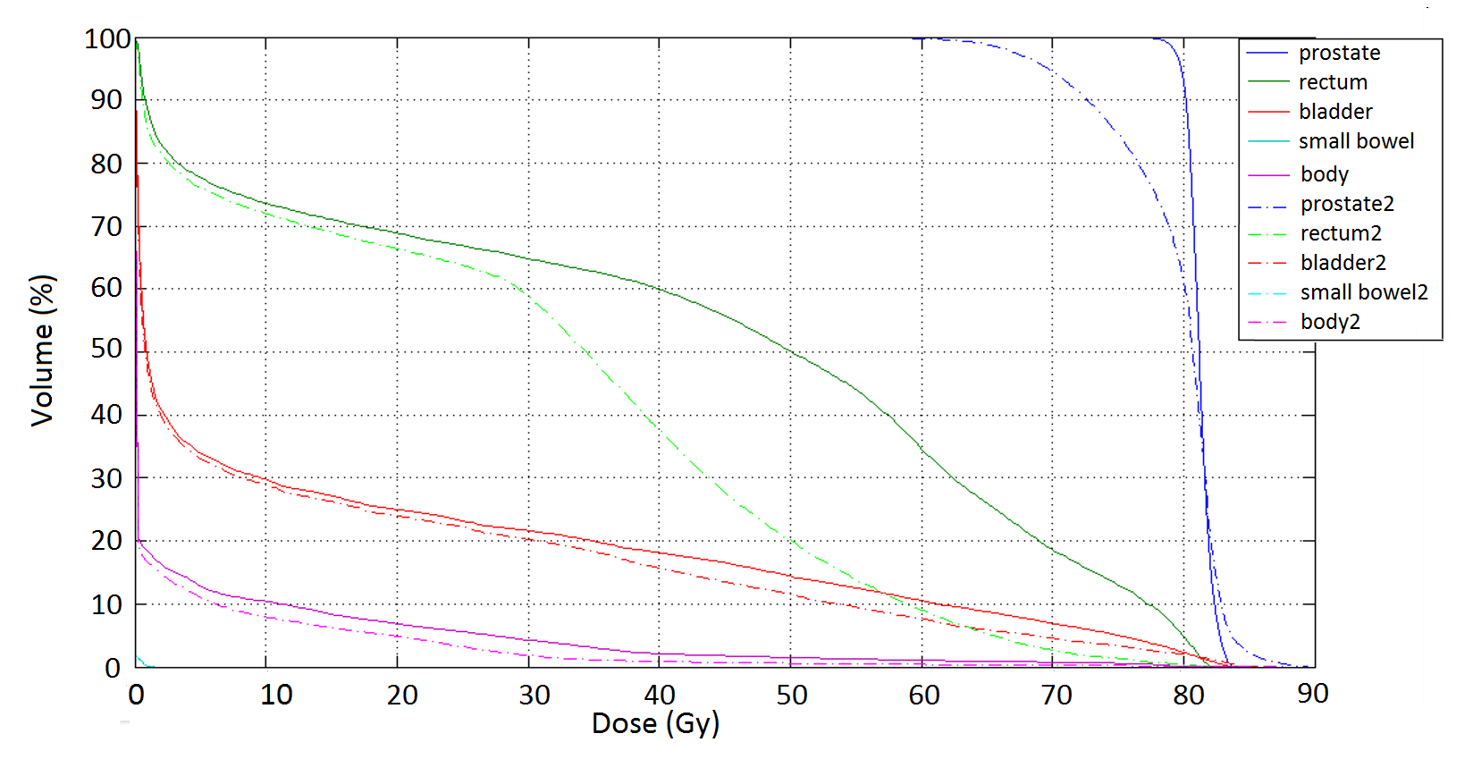
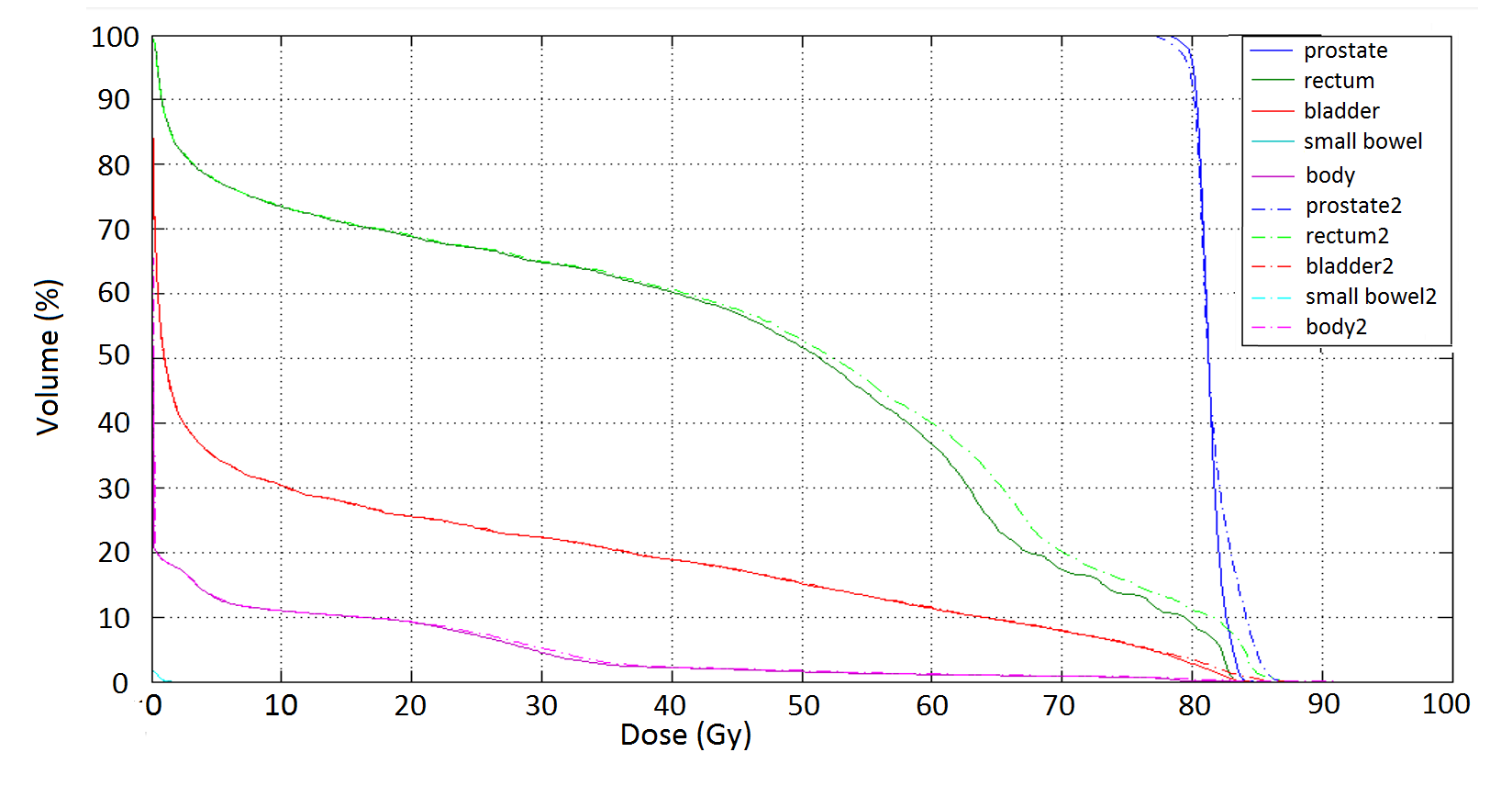
Figure 1. Dose volume histograms (DVH) of the two experiments. Solid lines represent the algorithm with TV-superiorization (broken lines represent the algorithm without TV-superiorization). The first (top) took 12 iterations and the second (bottom) took 7 iterations.

5. Conclusions

Our proposed method successfully produced conformal solutions that met the acceptance criteria while an otherwise identical algorithm without superiorization failed to do so with the same number of iterations. Future work will assess the computational gain of the superiorization method compared to a conventional method and investigate its utility for computationally more complex problems that can be found in modulated techniques for arc therapy.

Acknowledgements. This work is supported by the U.S. Department of Defense Prostate Cancer Research Program Award No. W81XWH-12-1-0122, by grant number 2009012 from the United States–Israel Binational Science Foundation (BSF) and by the U.S. Department of the Army Award No. W81XWH-10-1-0170. Some of the material was presented as a poster at the Technology for Innovation in Radiation Oncology, Joint Workshop of the American Society for Radiation Oncology (ASTRO), the National Cancer Institute (NCI) and the American Association of Physicists in Medicine (AAPM), National Institutes of Health (NIH), Bethesda, MD, USA, June 13–14, 2013.

References

- [A] K. Otto, Volumetric modulated arc therapy: IMRT in a single gantry arc, Medical Physics 35 (2008), 310–317.
- [B] S. Webb, The physical basis of IMRT and inverse planning, British Journal of Radiology 76 (2003), 678–689.
- [C] T. Bortfeld, IMRT: a review and preview, Physics in Medicine and Biology 51 (2006), R363–R379.
- [D] H.H. Bauschke and V.R. Koch, Projection methods: Swiss army knives for solving feasibility and best approximation problems with halfspaces, The Conference on Infinite Products and Their Applications (Technion, Haifa, Israel, 2012), Contemporary Mathematics, accepted for publication. http://arxiv.org/abs/1301.4506v1.
- [E] M.D. Altschuler and Y. Censor, Feasibility solutions in radiation therapy treatment planning, in: Proceedings of the Eighth International Conference on the Use of Computers in Radiation Therapy, IEEE Computer Society Press, Silver Spring, MD, USA (1984), 220–224.
- [F] Y. Censor, M.D. Altschuler and W.D. Powlis, A computational solution of the inverse problem in radiation-therapy treatment planning, Applied Mathematics and Computation 25 (1988), 57–87.
- [G] L. Zhu, L. Lee, Y. Ma, Y. Ye, R. Mazzeo and L. Xing, Using total-variation regularization for intensity modulated radiation therapy inverse planning with field-specific numbers of segments, Physics in Medicine and Biology 53 (2008), 6653–6672.
- [H] Y. Censor, R. Davidi, G.T. Herman, R.W. Schulte and L. Tetruashvili, Projected subgradient minimization versus superiorization, Journal of Optimization Theory and Applications, accepted for publication. DOI:10.1007/s10957-013-0408-3.
- [I] G.T. Herman, E. Garduño, R. Davidi and Y. Censor Superiorization: An optimization heuristic for medical physics, Medical Physics 39 (2012), 5532–5546.
-
[J]
Radiation Therapy Oncology Group: RTOG 0815
Protocol Information.
http://www.rtog.org/ClinicalTrials/ProtocolTable/StudyDetails.aspx?study=0815.Updated: 1/30/2014. - [K] G.T. Herman and A. Lent A family of iterative quadratic optimization algorithms for pairs of inequalities with application in diagnostic radiology, Mathematical Programming Studies 9 (1978), 15–29.
- [L] D. Butnariu, R. Davidi, G.T. Herman and I.G. Kazantsev Stable convergence behavior under summable perturbations of a class of projection methods for convex feasibility and optimization problems, IEEE Journal of Selected Topics In Signal Processing 1 (2007), 540–547.
- [M] K.T. Block , M. Uecker and J. Frahm Undersampled radial MRI with multiple coils. Iterative image reconstruction using a total variation constraint, Magnetic Resonance in Medicine 57 (2007), 1086–1098.
- [N] V. Kolehmainen, A. Vanne, S. Siltanen, S. Jrvenp, J.P. Kaipio, M. Lassas and M. Kalke Parallelized Bayesian inversion for three-dimensional dental x-ray imaging, IEEE Transactions on Medical Imaging 25 (2006), 218–228.
- [O] W. Chen, G.T. Herman and Y. Censor, Algorithms for satisfying dose-volume constraints in intensity-modulated radiation therapy, in: Y. Censor, M. Jiang and A.K. Louis (Editors), Mathematical Methods in Biomedical Imaging and Intensity-Modulated Radiation Therapy (IMRT), Edizioni della Normale, Pisa, Italy, (2008) 97–106.
- [P] C. Yu, Intensity-modulated arc therapy with dynamic multileaf collimation: an alternative to tomotherapy, Physics in Medicine and Biology 40 (1995), 1435–1449.
- [Q] S. M. Crooks and L. Xing, Application of constrained least-squares techniques to IMRT treatment planning, International Journal of Radiation Oncology, Biology and Physics 54 (2002), 1217–1224.