SISSA 04/2014/FISI

On the Validity of the Effective Field Theory
for Dark Matter Searches at the LHC
Part II: Complete Analysis for the s𝑠s-channel

Giorgio Busonia,111giorgio.busoni@sissa.it, Andrea De Simonea,222andrea.desimone@sissa.it,

Johanna Gramlingb,333johanna.gramling@unige.ch, Enrico Morganteb,444enrico.morgante@unige.ch, Antonio Riottob,555antonio.riotto@unige.ch

a SISSA and INFN, Sezione di Trieste, via Bonomea 265, I-34136 Trieste, Italy
b Section de Physique, Université de Genève,
24 quai E. Ansermet, CH-1211 Geneva, Switzerland

Abstract

We generalize in several directions our recent analysis of the limitations to the use of the effective field theory approach to study dark matter at the LHC. Firstly, we study the full list of operators connecting fermion DM to quarks and gluons, corresponding to integrating out a heavy mediator in the s𝑠s-channel; secondly, we provide analytical results for the validity of the EFT description for both s=8𝑠8\sqrt{s}=8 TeV and 141414 TeV; thirdly, we make use of a MonteCarlo event generator approach to assess the validity of our analytical conclusions. We apply our results to revisit the current collider bounds on the ultraviolet cut-off scale of the effective field theory and show that these bounds are weakened once the validity conditions of the effective field theory are imposed.

1 Introduction

While there are many cosmological and astrophysical evidences that our universe contains a sizable amount of dark Matter (DM), i.e. a component which clusters at small scales, its nature is still a mystery. Various considerations point towards the possibility that DM is made of neutral particles whose mass and interactions are dictated by physics in the electroweak energy range. If so, the DM relic density of these particles, assuming they were in thermal equilibrium during the evolution of the universe, turns out to be

(ΩDMh20.110)3×1026cm3/secσvann,subscriptΩDMsuperscript20.1103superscript1026superscriptcm3secsubscriptdelimited-⟨⟩𝜎𝑣ann\left(\frac{\Omega_{\rm DM}h^{2}}{0.110}\right)\approx\frac{3\times 10^{-26}{\rm cm}^{3}/{\rm sec}}{\langle\sigma v\rangle_{\rm ann}}, (1.1)

where σvannsubscriptdelimited-⟨⟩𝜎𝑣ann\langle\sigma v\rangle_{\rm ann} is the (thermally-averaged) annihilation cross section. A weak interaction strength provides the abundance in the right range measured by the Planck collaboration: ΩDM=0.315±0.0175subscriptΩDMplus-or-minus0.3150.0175\Omega_{\rm DM}=0.315\pm 0.0175 [1]. This numerical coincidence represents the main reason why it is generically believed that DM is made of weakly-interacting particles with a mass in the range (102104)superscript102superscript104(10^{2}-10^{4}) GeV.

Currently, there are several ways to search for such DM candidates. Apart from the indirect [2] and direct [3] searches, DM particles (if they are light enough) might reveal themselves in particle colliders, namely at the LHC. Many LHC searches for DM are based on the idea of looking at events with missing energy plus a single jet or photon, emitted from the initial state in pp𝑝𝑝pp collisions (for alternative kinds of DM searches at the LHC see e.g. Refs. [4, 5, 6, 7, 8, 9])

ppχ+χ¯+jet/photon,𝑝𝑝𝜒¯𝜒jetphotonpp\to\chi+\overline{\chi}+{\rm jet/photon}, (1.2)

where χ𝜒\chi indicates the DM particle. Several results are already available from two LHC collaborations [10, 11, 12, 13, 14, 15, 16, 17].

In order to avoid the overwhelming model-dependence introduced by the plethora of DM models discussed in the literature, DM searches at the LHC have made use of the Effective Field Theory (EFT) [18, 19, 20, 21, 22, 23, 24, 25, 26, 27, 28]. This approach is a very powerful and economical way to grasp the main features of a physical process, only in terms of the degrees of freedom which are excited at the scale of the process. EFT techniques are successfully applied in many branches of physics, and in particular they have become a standard way to present experimental results for DM searches.

However, as far as collider searches are concerned, with the LHC being such a powerful machine, it is not guaranteed that the events used to constrain an effective interaction are not occurring at an energy scale larger than the cutoff scale of the effective description. In other words, some (or many) events of DM production may occur with such a high momentum transfer that the EFT is not a good description anymore. The question about the validity of the EFT for collider searches of DM has become pressing (see also Refs. [29, 30, 21, 31, 7, 32, 33, 34, 35]), especially in the perspective of analysing the data from the future LHC run at (13-14) TeV.

Let us consider a simple model where there is a heavy mediator of mass M𝑀M, to which the quarks and DM are coupled with couplings gqsubscript𝑔𝑞g_{q} and gχsubscript𝑔𝜒g_{\chi}, respectively. The EFT is a good approximation only at low energies. Indeed, it is possible at low energies to integrate out the heavy mediator from the theory and obtain a tower of operators. The matching condition of the ultra-violet (UV) theory with the mediator and its low-energy effective counterpart implies Λ=M/gqgχΛ𝑀subscript𝑔𝑞subscript𝑔𝜒\Lambda={M}/{\sqrt{g_{q}g_{\chi}}}. A DM production event occurs at an energy at which the EFT is reliable as long as Qtr<Msubscript𝑄tr𝑀Q_{\rm tr}<M, where Qtrsubscript𝑄trQ_{\rm tr} is the momentum transfer in the process; this, together with the condition of perturbativity of the couplings gq,χ<4πsubscript𝑔𝑞𝜒4𝜋g_{q,\chi}<4\pi, implies

Λ>Qtrgqgχ>Qtr4π.Λsubscript𝑄trsubscript𝑔𝑞subscript𝑔𝜒subscript𝑄tr4𝜋\Lambda>\frac{Q_{\rm tr}}{\sqrt{g_{q}g_{\chi}}}>\frac{Q_{\rm tr}}{4\pi}\,. (1.3)

If, in addition, one assumes the momentum transfer to occur in the s𝑠s-channel, then kinematics imposes Qtr>2mDMsubscript𝑄tr2subscript𝑚DMQ_{\rm tr}>2m_{\rm DM}, so Eq. (1.3) becomes

Λ>mDM2π.Λsubscript𝑚DM2𝜋\Lambda>\frac{m_{\rm DM}}{2\pi}\,. (1.4)

This is a very minimal requirement which is refined event-by-event by the stronger condition Eq. (1.3), which depends on mDMsubscript𝑚DMm_{\rm DM} through Qtrsubscript𝑄trQ_{\rm tr}. It is clear that the details of condition (1.3) depend on the values of the couplings in the UV theory. In the following, for definiteness, we will mostly identify the mass of the new degrees of freedom M𝑀M with the suppression scale of the operator ΛΛ\Lambda. This is equivalent to consider couplings in the UV theory of 𝒪(1)𝒪1{\cal O}(1). So, we will deal with the condition (but we will discuss also the impact of taking couplings larger than 1)

QtrΛ.less-than-or-similar-tosubscript𝑄trΛQ_{\rm tr}\lesssim\Lambda\,. (1.5)

In Ref. [29] we have started the discussion of the limitations to the use of the EFT approach for DM searches at the LHC by adopting a toy model where the heavy mediator is exchanged in the s𝑠s-channel and by introducing a few quantities which quantify the error made when using effective operators to describe processes with very high momentum transfer. Our criteria indicated up to what cutoff energy scale, and with what precision, the effective description is valid, depending on the DM mass and couplings. In this paper we significantly extend our previous work along four different directions:

  1. 1.

    we consider the full list of operators connecting fermion DM to quarks and corresponding to integrating out the heavy mediator in the s𝑠s-channel;

  2. 2.

    we provide analytical results for the validity of the EFT description for both s=8𝑠8\sqrt{s}=8 TeV and 141414 TeV;

  3. 3.

    we follow a MonteCarlo approach to assess the validity of the EFT and compare this fully numerical results with the analytical calculations;

  4. 4.

    we apply our results to revisit the current experimental bounds on the effective operator scale; by requiring that only the events which are “safe” from the EFT point of view should be considered, the bounds get weakened.

The rest of the present paper is organized as follows. In Section 2 we present and discuss the results of our analytical approach to assess the validity of EFT. In Section 3, the fully numerical approach is described and the results are compared with the analytical calculations. In Section 4 we analyze the impact of the limitation of the validity of the EFT for the current limits from the LHC searches. Finally, we draw our conclusions in Section 5. The details of the analytical results can be found in the Appendix A.

2 Validity of the EFT: analytical approach

2.1 Operators and cross sections

The starting point of our analysis is the list of the 18 operators reported in Tab. 1 which are commonly used in the literature [18]. We have considered not only the operators connecting the DM fermion to quarks (D1-D10), but also those involving gluon field strengths (D11-D14). Furthermore, the operators can originate from heavy mediators exchange in the s𝑠s-channel. For instance, the D1’ (D5) operators may be originated by the tree-level s𝑠s-channel exchange of a very heavy scalar (vector) boson S𝑆S (Vμsubscript𝑉𝜇V_{\mu}), with lagrangians

D1subscriptsuperscriptD1\displaystyle\mathscr{L}_{\rm D1^{\prime}} superset-of\displaystyle\supset 12M2S2gqq¯qSgχχ¯χS,12superscript𝑀2superscript𝑆2subscript𝑔𝑞¯𝑞𝑞𝑆subscript𝑔𝜒¯𝜒𝜒𝑆\displaystyle\frac{1}{2}M^{2}S^{2}-g_{q}\bar{q}qS-g_{\chi}\bar{\chi}\chi S\,, (2.1)
D5subscriptD5\displaystyle\mathscr{L}_{\rm D5} superset-of\displaystyle\supset 12M2VμVμgqq¯γμqVμgχχ¯γμχVμ.12superscript𝑀2superscript𝑉𝜇subscript𝑉𝜇subscript𝑔𝑞¯𝑞superscript𝛾𝜇𝑞subscript𝑉𝜇subscript𝑔𝜒¯𝜒superscript𝛾𝜇𝜒subscript𝑉𝜇\displaystyle\frac{1}{2}M^{2}V^{\mu}V_{\mu}-g_{q}\bar{q}\gamma^{\mu}qV_{\mu}-g_{\chi}\bar{\chi}\gamma^{\mu}\chi V_{\mu}\,. (2.2)

Notice the presence of the “primed” operators D1𝐷superscript1D1^{\prime}D4𝐷superscript4D4^{\prime}, very similar to the ones often considered D1𝐷1D1D4𝐷4D4, respectively, but with a different normalization, independent of the quark masses. In fact, they may arise from integrating out heavy scalars which do not take a vacuum expectation value and therefore do not give rise to quark masses. 111 A normalization proportional to the quark mass is common in many models motivated by flavour physics, but in general the coefficient Λ3superscriptΛ3\Lambda^{3} at the denominator can have a different form. For example, if the effective operators come from a Naturalness-motivated new physics theory like Supersymmetry or Composite Higgs Models, assuming a U(2)3𝑈superscript23U(2)^{3} flavour symmetry [36, 37] the normalization would be λt,b1Λ2mqmt,bsubscript𝜆𝑡𝑏1superscriptΛ2subscript𝑚𝑞subscript𝑚𝑡𝑏\lambda_{t,b}\frac{1}{\Lambda^{2}}\frac{m_{q}}{m_{t,b}} (2.3) where ΛΛ\Lambda is an energy scale of the order some TeV related to the Electroweak Symmetry Breaking and mt,b,λt,bsubscript𝑚𝑡𝑏subscript𝜆𝑡𝑏m_{t,b},\lambda_{t,b} are the mass and the Yukawa coupling with the Higgs of the top/bottom quark, depending on whether the quark q𝑞q is up-like or down-like. In the present work, we will be agnostic about this point, and we’ll keep both the primed and unprimed operators into account on the same footing as all others.

Name Operator Coefficient
D1 χ¯χq¯q¯𝜒𝜒¯𝑞𝑞\bar{\chi}\chi\;\bar{q}q mq/Λ3subscript𝑚𝑞superscriptΛ3{m_{q}}/{\Lambda^{3}}
D1’ χ¯χq¯q¯𝜒𝜒¯𝑞𝑞\bar{\chi}\chi\;\bar{q}q 1/Λ21superscriptΛ2{1}/{\Lambda^{2}}
D2 χ¯γ5χq¯q¯𝜒superscript𝛾5𝜒¯𝑞𝑞\bar{\chi}\gamma^{5}\chi\;\bar{q}q imq/Λ3𝑖subscript𝑚𝑞superscriptΛ3i{m_{q}}/{\Lambda^{3}}
D2’ χ¯γ5χq¯q¯𝜒superscript𝛾5𝜒¯𝑞𝑞\bar{\chi}\gamma^{5}\chi\;\bar{q}q i/Λ2𝑖superscriptΛ2{i}/{\Lambda^{2}}
D3 χ¯χq¯γ5q¯𝜒𝜒¯𝑞superscript𝛾5𝑞\bar{\chi}\chi\;\bar{q}\gamma^{5}q imq/Λ3𝑖subscript𝑚𝑞superscriptΛ3i{m_{q}}/{\Lambda^{3}}
D3’ χ¯χq¯γ5q¯𝜒𝜒¯𝑞superscript𝛾5𝑞\bar{\chi}\chi\;\bar{q}\gamma^{5}q i/Λ2𝑖superscriptΛ2{i}/{\Lambda^{2}}
D4 χ¯γ5χq¯γ5q¯𝜒superscript𝛾5𝜒¯𝑞superscript𝛾5𝑞\bar{\chi}\gamma^{5}\chi\;\bar{q}\gamma^{5}q mq/Λ3subscript𝑚𝑞superscriptΛ3{m_{q}}/{\Lambda^{3}}
D4’ χ¯γ5χq¯γ5q¯𝜒superscript𝛾5𝜒¯𝑞superscript𝛾5𝑞\bar{\chi}\gamma^{5}\chi\;\bar{q}\gamma^{5}q 1/Λ21superscriptΛ2{1}/{\Lambda^{2}}
D5 χ¯γμχq¯γμq¯𝜒subscript𝛾𝜇𝜒¯𝑞superscript𝛾𝜇𝑞\bar{\chi}\gamma_{\mu}\chi\;\bar{q}\gamma^{\mu}q 1/Λ21superscriptΛ2{1}/{\Lambda^{2}}
D6 χ¯γμγ5χq¯γμq¯𝜒subscript𝛾𝜇superscript𝛾5𝜒¯𝑞superscript𝛾𝜇𝑞\bar{\chi}\gamma_{\mu}\gamma^{5}\chi\;\bar{q}\gamma^{\mu}q 1/Λ21superscriptΛ2{1}/{\Lambda^{2}}
D7 χ¯γμχq¯γμγ5q¯𝜒subscript𝛾𝜇𝜒¯𝑞superscript𝛾𝜇superscript𝛾5𝑞\bar{\chi}\gamma_{\mu}\chi\;\bar{q}\gamma^{\mu}\gamma^{5}q 1/Λ21superscriptΛ2{1}/{\Lambda^{2}}
D8 χ¯γμγ5χq¯γμγ5q¯𝜒subscript𝛾𝜇superscript𝛾5𝜒¯𝑞superscript𝛾𝜇superscript𝛾5𝑞\bar{\chi}\gamma_{\mu}\gamma^{5}\chi\;\bar{q}\gamma^{\mu}\gamma^{5}q 1/Λ21superscriptΛ2{1}/{\Lambda^{2}}
D9 χ¯σμνχq¯σμνq¯𝜒subscript𝜎𝜇𝜈𝜒¯𝑞superscript𝜎𝜇𝜈𝑞\bar{\chi}\sigma_{\mu\nu}\chi\;\bar{q}\sigma^{\mu\nu}q 1/Λ21superscriptΛ2{1}/{\Lambda^{2}}
D10 χ¯σμνγ5χq¯σμνq¯𝜒subscript𝜎𝜇𝜈superscript𝛾5𝜒¯𝑞superscript𝜎𝜇𝜈𝑞\bar{\chi}\sigma_{\mu\nu}\gamma^{5}\chi\;\bar{q}\sigma^{\mu\nu}q\; i/Λ2𝑖superscriptΛ2{i}/{\Lambda^{2}}
D11 χ¯χGμνGμν¯𝜒𝜒superscript𝐺𝜇𝜈subscript𝐺𝜇𝜈\bar{\chi}\chi\;G^{\mu\nu}G_{\mu\nu}\; αs/4Λ3subscript𝛼𝑠4superscriptΛ3{\alpha_{s}}/{4\Lambda^{3}}
D12 χ¯γ5χGμνGμν¯𝜒superscript𝛾5𝜒superscript𝐺𝜇𝜈subscript𝐺𝜇𝜈\bar{\chi}\gamma^{5}\chi\;G^{\mu\nu}G_{\mu\nu}\; iαs/4Λ3𝑖subscript𝛼𝑠4superscriptΛ3{i\alpha_{s}}/{4\Lambda^{3}}
D13 χ¯χGμνG~μν¯𝜒𝜒superscript𝐺𝜇𝜈subscript~𝐺𝜇𝜈\bar{\chi}\chi\;G^{\mu\nu}\tilde{G}_{\mu\nu}\; iαs/4Λ3𝑖subscript𝛼𝑠4superscriptΛ3{i\alpha_{s}}/{4\Lambda^{3}}
D14 χ¯γ5χGμνG~μν¯𝜒superscript𝛾5𝜒superscript𝐺𝜇𝜈subscript~𝐺𝜇𝜈\bar{\chi}\gamma^{5}\chi\;G^{\mu\nu}\tilde{G}_{\mu\nu}\; αs/4Λ3subscript𝛼𝑠4superscriptΛ3{\alpha_{s}}/{4\Lambda^{3}}
Table 1: Operators used throughout this work. The nomenclature is mostly taken from Ref. [21].

We have computed the tree-level differential cross sections in the transverse momentum pTsubscript𝑝Tp_{\rm T} and rapidity η𝜂\eta of the final jet for the hard scattering process with gluon radiation from the initial state f(p1)+f¯(p2)χ(p3)+χ(p4)+g(k)𝑓subscript𝑝1¯𝑓subscript𝑝2𝜒subscript𝑝3𝜒subscript𝑝4𝑔𝑘f(p_{1})+\bar{f}(p_{2})\to\chi(p_{3})+\chi(p_{4})+g(k), where f𝑓f is either a quark (for operators D1-D10), or a gluon (for operators D11-D14). The results are conveniently written in terms of the momentum transfer in the s𝑠s-channel

Qtr2=(p1+p2k)2=x1x2sspT(x1eη+x2eη),superscriptsubscript𝑄tr2superscriptsubscript𝑝1subscript𝑝2𝑘2subscript𝑥1subscript𝑥2𝑠𝑠subscript𝑝Tsubscript𝑥1superscript𝑒𝜂subscript𝑥2superscript𝑒𝜂Q_{\rm tr}^{2}=(p_{1}+p_{2}-k)^{2}={x_{1}x_{2}s}-\sqrt{s}\,p_{\rm T}\left(x_{1}e^{-\eta}+x_{2}e^{\eta}\right)\,, (2.4)

where x1,x2subscript𝑥1subscript𝑥2x_{1},x_{2} are the fractions of momentum carried by initial partons and η,pT𝜂subscript𝑝T\eta,p_{\rm T} are the pseudo-rapidity and the transverse momentum of the final state gluon, respectively. The expressions are of course valid for all admitted values of the parameters. It’s only when integrated numerically over the PDFs and over η,pT𝜂subscript𝑝T\eta,p_{\rm T} that the dependence on these values comes in. We obtain

d2σ^dpTdη|D1evaluated-atsuperscriptd2^𝜎dsubscript𝑝Td𝜂𝐷superscript1\displaystyle\left.\dfrac{\textrm{d}^{2}\hat{\sigma}}{\textrm{d}p_{\rm T}\textrm{d}\eta}\right|_{D1^{\prime}} =\displaystyle= αs36π21pT1Λ4[Qtr24mDM2]3/2[1+Qtr4(x1x2s)2]Qtr,subscript𝛼𝑠36superscript𝜋21subscript𝑝T1superscriptΛ4superscriptdelimited-[]superscriptsubscript𝑄tr24superscriptsubscript𝑚DM232delimited-[]1superscriptsubscript𝑄tr4superscriptsubscript𝑥1subscript𝑥2𝑠2subscript𝑄tr\displaystyle\frac{\alpha_{s}}{36\pi^{2}}\frac{1}{p_{\rm T}}\frac{1}{\Lambda^{4}}\frac{\left[Q_{\rm tr}^{2}-4m_{\rm DM}^{2}\right]^{3/2}\left[1+\frac{Q_{\rm tr}^{4}}{(x_{1}x_{2}s)^{2}}\right]}{\,Q_{\rm tr}}\,, (2.5)
d2σ^dpTdη|D4evaluated-atsuperscriptd2^𝜎dsubscript𝑝Td𝜂𝐷superscript4\displaystyle\left.\dfrac{\textrm{d}^{2}\hat{\sigma}}{\textrm{d}p_{\rm T}\textrm{d}\eta}\right|_{D4^{\prime}} =\displaystyle= αs36π21pT1Λ4Qtr[Qtr24mDM2]1/2[1+Qtr4(x1x2s)2],subscript𝛼𝑠36superscript𝜋21subscript𝑝T1superscriptΛ4subscript𝑄trsuperscriptdelimited-[]superscriptsubscript𝑄tr24superscriptsubscript𝑚DM212delimited-[]1superscriptsubscript𝑄tr4superscriptsubscript𝑥1subscript𝑥2𝑠2\displaystyle\frac{\alpha_{s}}{36\pi^{2}}\frac{1}{p_{\rm T}}\frac{1}{\Lambda^{4}}Q_{\rm tr}\left[Q_{\rm tr}^{2}-4m_{\rm DM}^{2}\right]^{1/2}\left[1+\frac{Q_{\rm tr}^{4}}{(x_{1}x_{2}s)^{2}}\right]\,, (2.6)
d2σ^dpTdη|D5evaluated-atsuperscriptd2^𝜎dsubscript𝑝Td𝜂𝐷5\displaystyle\left.\dfrac{\textrm{d}^{2}\hat{\sigma}}{\textrm{d}p_{\rm T}\textrm{d}\eta}\right|_{D5} =\displaystyle= αs27π21pT1Λ4[Qtr24mDM2]1/2[Qtr2+2mDM2][1+Qtr4(x1x2s)22pT2x1x2s]Qtr,subscript𝛼𝑠27superscript𝜋21subscript𝑝T1superscriptΛ4superscriptdelimited-[]superscriptsubscript𝑄tr24superscriptsubscript𝑚DM212delimited-[]superscriptsubscript𝑄tr22superscriptsubscript𝑚DM2delimited-[]1superscriptsubscript𝑄tr4superscriptsubscript𝑥1subscript𝑥2𝑠22superscriptsubscript𝑝T2subscript𝑥1subscript𝑥2𝑠subscript𝑄tr\displaystyle\frac{\alpha_{s}}{27\pi^{2}}\frac{1}{p_{\rm T}}\frac{1}{\Lambda^{4}}\frac{\left[Q_{\rm tr}^{2}-4m_{\rm DM}^{2}\right]^{1/2}\left[Q_{\rm tr}^{2}+2m_{\rm DM}^{2}\right]\left[1+\frac{Q_{\rm tr}^{4}}{(x_{1}x_{2}s)^{2}}-2\frac{p_{\rm T}^{2}}{x_{1}x_{2}s}\right]}{\,Q_{\rm tr}}\,, (2.7)
d2σ^dpTdη|D8evaluated-atsuperscriptd2^𝜎dsubscript𝑝Td𝜂𝐷8\displaystyle\left.\dfrac{\textrm{d}^{2}\hat{\sigma}}{\textrm{d}p_{\rm T}\textrm{d}\eta}\right|_{D8} =\displaystyle= αs27π21pT1Λ4[Qtr24mDM2]3/2[1+Qtr4(x1x2s)22pT2x1x2s]Qtr,subscript𝛼𝑠27superscript𝜋21subscript𝑝T1superscriptΛ4superscriptdelimited-[]superscriptsubscript𝑄tr24superscriptsubscript𝑚DM232delimited-[]1superscriptsubscript𝑄tr4superscriptsubscript𝑥1subscript𝑥2𝑠22superscriptsubscript𝑝T2subscript𝑥1subscript𝑥2𝑠subscript𝑄tr\displaystyle\frac{\alpha_{s}}{27\pi^{2}}\frac{1}{p_{\rm T}}\frac{1}{\Lambda^{4}}\frac{\left[Q_{\rm tr}^{2}-4m_{\rm DM}^{2}\right]^{3/2}\left[1+\frac{Q_{\rm tr}^{4}}{(x_{1}x_{2}s)^{2}}-2\frac{p_{\rm T}^{2}}{x_{1}x_{2}s}\right]}{\,Q_{\rm tr}}\,, (2.8)
d2σ^dpTdη|D9evaluated-atsuperscriptd2^𝜎dsubscript𝑝Td𝜂𝐷9\displaystyle\left.\dfrac{\textrm{d}^{2}\hat{\sigma}}{\textrm{d}p_{\rm T}\textrm{d}\eta}\right|_{D9} =\displaystyle= 2αs27π21pT1Λ4Qtr4mDM2[Qtr2+2mDM2][1+Qtr4(x1x2s)2+4pT2(1Qtr21x1x2s)]Qtr,2subscript𝛼𝑠27superscript𝜋21subscript𝑝T1superscriptΛ4subscript𝑄tr4superscriptsubscript𝑚DM2delimited-[]superscriptsubscript𝑄tr22superscriptsubscript𝑚DM2delimited-[]1superscriptsubscript𝑄tr4superscriptsubscript𝑥1subscript𝑥2𝑠24superscriptsubscript𝑝T21superscriptsubscript𝑄tr21subscript𝑥1subscript𝑥2𝑠subscript𝑄tr\displaystyle\frac{2\alpha_{s}}{27\pi^{2}}\frac{1}{p_{\rm T}}\frac{1}{\Lambda^{4}}\frac{\sqrt{Q_{\rm tr}-4m_{\rm DM}^{2}}\left[Q_{\rm tr}^{2}+2m_{\rm DM}^{2}\right]\left[1+\frac{Q_{\rm tr}^{4}}{(x_{1}x_{2}s)^{2}}+4p_{\rm T}^{2}\left(\frac{1}{Q_{\rm tr}^{2}}-\frac{1}{x_{1}x_{2}s}\right)\right]}{\,Q_{\rm tr}}\,,
d2σ^dpTdη|D11evaluated-atsuperscriptd2^𝜎dsubscript𝑝Td𝜂𝐷11\displaystyle\left.\dfrac{\textrm{d}^{2}\hat{\sigma}}{\textrm{d}p_{\rm T}\textrm{d}\eta}\right|_{D11} =\displaystyle= 3αs3256π2Λ6(x1x2s)3(Qtr2x1x2s)2(Qtr24mDM2)3/2pTQtr[14Qtr2pT2x1x2s+8Qtr4+21pT4(x1x2s)2\displaystyle\frac{3\alpha_{s}^{3}}{256\pi^{2}\Lambda^{6}}\frac{(x_{1}x_{2}s)^{3}}{(Q_{\rm tr}^{2}-x_{1}x_{2}s)^{2}}\frac{(Q_{\rm tr}^{2}-4m_{\rm DM}^{2})^{3/2}}{p_{\rm T}Q_{\rm tr}}\left[1-4\frac{Q_{\rm tr}^{2}-p_{\rm T}^{2}}{x_{1}x_{2}s}+\frac{8Q_{\rm tr}^{4}+21p_{\rm T}^{4}}{(x_{1}x_{2}s)^{2}}\right. (2.10)
2Qtr25Qtr4+4Qtr2pT2+5pT4(x1x2s)3+Qtr48Qtr4+8Qtr2pT2+5pT4(x1x2s)44Qtr8Qtr2+pT2(x1x2s)52superscriptsubscript𝑄tr25superscriptsubscript𝑄tr44superscriptsubscript𝑄tr2superscriptsubscript𝑝T25superscriptsubscript𝑝T4superscriptsubscript𝑥1subscript𝑥2𝑠3superscriptsubscript𝑄tr48superscriptsubscript𝑄tr48superscriptsubscript𝑄tr2superscriptsubscript𝑝T25superscriptsubscript𝑝T4superscriptsubscript𝑥1subscript𝑥2𝑠44superscriptsubscript𝑄tr8superscriptsubscript𝑄tr2superscriptsubscript𝑝T2superscriptsubscript𝑥1subscript𝑥2𝑠5\displaystyle-2Q_{\rm tr}^{2}\frac{5Q_{\rm tr}^{4}+4Q_{\rm tr}^{2}p_{\rm T}^{2}+5p_{\rm T}^{4}}{(x_{1}x_{2}s)^{3}}+Q_{\rm tr}^{4}\frac{8Q_{\rm tr}^{4}+8Q_{\rm tr}^{2}p_{\rm T}^{2}+5p_{\rm T}^{4}}{(x_{1}x_{2}s)^{4}}-4Q_{\rm tr}^{8}\frac{Q_{\rm tr}^{2}+p_{\rm T}^{2}}{(x_{1}x_{2}s)^{5}}
+Qtr12(x1x2s)6],\displaystyle\left.+\frac{Q_{\rm tr}^{12}}{(x_{1}x_{2}s)^{6}}\right]\,,
d2σ^dpTdη|D12evaluated-atsuperscriptd2^𝜎dsubscript𝑝Td𝜂𝐷12\displaystyle\left.\dfrac{\textrm{d}^{2}\hat{\sigma}}{\textrm{d}p_{\rm T}\textrm{d}\eta}\right|_{D12} =\displaystyle= 3αs3256π2Λ6(x1x2s)3(Qtr2x1x2s)2QtrQtr24mDM2pT[14Qtr2pT2x1x2s+8Qtr4+21pT4(x1x2s)2\displaystyle\frac{3\alpha_{s}^{3}}{256\pi^{2}\Lambda^{6}}\frac{(x_{1}x_{2}s)^{3}}{(Q_{\rm tr}^{2}-x_{1}x_{2}s)^{2}}\frac{Q_{\rm tr}\sqrt{Q_{\rm tr}^{2}-4m_{\rm DM}^{2}}}{p_{\rm T}}\left[1-4\frac{Q_{\rm tr}^{2}-p_{\rm T}^{2}}{x_{1}x_{2}s}+\frac{8Q_{\rm tr}^{4}+21p_{\rm T}^{4}}{(x_{1}x_{2}s)^{2}}\right. (2.11)
2Qtr25Qtr4+4Qtr2pT2+5pT4(x1x2s)3+Qtr48Qtr4+8Qtr2pT2+5pT4(x1x2s)44Qtr8Qtr2+pT2(x1x2s)52superscriptsubscript𝑄tr25superscriptsubscript𝑄tr44superscriptsubscript𝑄tr2superscriptsubscript𝑝T25superscriptsubscript𝑝T4superscriptsubscript𝑥1subscript𝑥2𝑠3superscriptsubscript𝑄tr48superscriptsubscript𝑄tr48superscriptsubscript𝑄tr2superscriptsubscript𝑝T25superscriptsubscript𝑝T4superscriptsubscript𝑥1subscript𝑥2𝑠44superscriptsubscript𝑄tr8superscriptsubscript𝑄tr2superscriptsubscript𝑝T2superscriptsubscript𝑥1subscript𝑥2𝑠5\displaystyle-2Q_{\rm tr}^{2}\frac{5Q_{\rm tr}^{4}+4Q_{\rm tr}^{2}p_{\rm T}^{2}+5p_{\rm T}^{4}}{(x_{1}x_{2}s)^{3}}+Q_{\rm tr}^{4}\frac{8Q_{\rm tr}^{4}+8Q_{\rm tr}^{2}p_{\rm T}^{2}+5p_{\rm T}^{4}}{(x_{1}x_{2}s)^{4}}-4Q_{\rm tr}^{8}\frac{Q_{\rm tr}^{2}+p_{\rm T}^{2}}{(x_{1}x_{2}s)^{5}}
+Qtr12(x1x2s)6],\displaystyle\left.+\frac{Q_{\rm tr}^{12}}{(x_{1}x_{2}s)^{6}}\right]\,,
d2σ^dpTdη|D13evaluated-atsuperscriptd2^𝜎dsubscript𝑝Td𝜂𝐷13\displaystyle\left.\dfrac{\textrm{d}^{2}\hat{\sigma}}{\textrm{d}p_{\rm T}\textrm{d}\eta}\right|_{D13} =\displaystyle= 3αs3256π2Λ6(x1x2s)3(Qtr2x1x2s)2(Qtr24mDM2)3/2pTQtr[14Qtr2x1x2s+8Qtr4+8Qtr2pT2+5pT4(x1x2s)2\displaystyle\frac{3\alpha_{s}^{3}}{256\pi^{2}\Lambda^{6}}\frac{(x_{1}x_{2}s)^{3}}{(Q_{\rm tr}^{2}-x_{1}x_{2}s)^{2}}\frac{(Q_{\rm tr}^{2}-4m_{\rm DM}^{2})^{3/2}}{p_{\rm T}Q_{\rm tr}}\left[1-4\frac{Q_{\rm tr}^{2}}{x_{1}x_{2}s}+\frac{8Q_{\rm tr}^{4}+8Q_{\rm tr}^{2}p_{\rm T}^{2}+5p_{\rm T}^{4}}{(x_{1}x_{2}s)^{2}}\right. (2.12)
2Qtr25Qtr4+6Qtr2pT23pT4(x1x2s)3+Qtr48Qtr4+8Qtr2pT2+5pT4(x1x2s)44Qtr8Qtr2+pT2(x1x2s)52superscriptsubscript𝑄tr25superscriptsubscript𝑄tr46superscriptsubscript𝑄tr2superscriptsubscript𝑝T23superscriptsubscript𝑝T4superscriptsubscript𝑥1subscript𝑥2𝑠3superscriptsubscript𝑄tr48superscriptsubscript𝑄tr48superscriptsubscript𝑄tr2superscriptsubscript𝑝T25superscriptsubscript𝑝T4superscriptsubscript𝑥1subscript𝑥2𝑠44superscriptsubscript𝑄tr8superscriptsubscript𝑄tr2superscriptsubscript𝑝T2superscriptsubscript𝑥1subscript𝑥2𝑠5\displaystyle-2Q_{\rm tr}^{2}\frac{5Q_{\rm tr}^{4}+6Q_{\rm tr}^{2}p_{\rm T}^{2}-3p_{\rm T}^{4}}{(x_{1}x_{2}s)^{3}}+Q_{\rm tr}^{4}\frac{8Q_{\rm tr}^{4}+8Q_{\rm tr}^{2}p_{\rm T}^{2}+5p_{\rm T}^{4}}{(x_{1}x_{2}s)^{4}}-4Q_{\rm tr}^{8}\frac{Q_{\rm tr}^{2}+p_{\rm T}^{2}}{(x_{1}x_{2}s)^{5}}
+Qtr12(x1x2s)6],\displaystyle\left.+\frac{Q_{\rm tr}^{12}}{(x_{1}x_{2}s)^{6}}\right]\,,
d2σ^dpTdη|D14evaluated-atsuperscriptd2^𝜎dsubscript𝑝Td𝜂𝐷14\displaystyle\left.\dfrac{\textrm{d}^{2}\hat{\sigma}}{\textrm{d}p_{\rm T}\textrm{d}\eta}\right|_{D14} =\displaystyle= 3αs3256π2Λ6(x1x2s)3(Qtr2x1x2s)2QtrQtr24mDM2pT[14Qtr2x1x2s+8Qtr4+8Qtr2pT2+5pT4(x1x2s)2\displaystyle\frac{3\alpha_{s}^{3}}{256\pi^{2}\Lambda^{6}}\frac{(x_{1}x_{2}s)^{3}}{(Q_{\rm tr}^{2}-x_{1}x_{2}s)^{2}}\frac{Q_{\rm tr}\sqrt{Q_{\rm tr}^{2}-4m_{\rm DM}^{2}}}{p_{\rm T}}\left[1-4\frac{Q_{\rm tr}^{2}}{x_{1}x_{2}s}+\frac{8Q_{\rm tr}^{4}+8Q_{\rm tr}^{2}p_{\rm T}^{2}+5p_{\rm T}^{4}}{(x_{1}x_{2}s)^{2}}\right. (2.13)
2Qtr25Qtr4+6Qtr2pT23pT4(x1x2s)3+Qtr48Qtr4+8Qtr2pT2+5pT4(x1x2s)44Qtr8Qtr2+pT2(x1x2s)52superscriptsubscript𝑄tr25superscriptsubscript𝑄tr46superscriptsubscript𝑄tr2superscriptsubscript𝑝T23superscriptsubscript𝑝T4superscriptsubscript𝑥1subscript𝑥2𝑠3superscriptsubscript𝑄tr48superscriptsubscript𝑄tr48superscriptsubscript𝑄tr2superscriptsubscript𝑝T25superscriptsubscript𝑝T4superscriptsubscript𝑥1subscript𝑥2𝑠44superscriptsubscript𝑄tr8superscriptsubscript𝑄tr2superscriptsubscript𝑝T2superscriptsubscript𝑥1subscript𝑥2𝑠5\displaystyle-2Q_{\rm tr}^{2}\frac{5Q_{\rm tr}^{4}+6Q_{\rm tr}^{2}p_{\rm T}^{2}-3p_{\rm T}^{4}}{(x_{1}x_{2}s)^{3}}+Q_{\rm tr}^{4}\frac{8Q_{\rm tr}^{4}+8Q_{\rm tr}^{2}p_{\rm T}^{2}+5p_{\rm T}^{4}}{(x_{1}x_{2}s)^{4}}-4Q_{\rm tr}^{8}\frac{Q_{\rm tr}^{2}+p_{\rm T}^{2}}{(x_{1}x_{2}s)^{5}}
+Qtr12(x1x2s)6].\displaystyle\left.+\frac{Q_{\rm tr}^{12}}{(x_{1}x_{2}s)^{6}}\right]\,.

The reader can find the details of the derivation of Eqs. (2.5)-(2.13) in Appendix A. As for the other operators, we get

d2σ^dpTdη|D2=d2σ^dpTdη|D4evaluated-atsuperscriptd2^𝜎dsubscript𝑝Td𝜂𝐷superscript2evaluated-atsuperscriptd2^𝜎dsubscript𝑝Td𝜂𝐷superscript4\displaystyle\left.\dfrac{\textrm{d}^{2}\hat{\sigma}}{\textrm{d}p_{\rm T}\textrm{d}\eta}\right|_{D2^{\prime}}=\left.\dfrac{\textrm{d}^{2}\hat{\sigma}}{\textrm{d}p_{\rm T}\textrm{d}\eta}\right|_{D4^{\prime}}\qquad d2σ^dpTdη|D3=d2σ^dpTdη|D1evaluated-atsuperscriptd2^𝜎dsubscript𝑝Td𝜂𝐷superscript3evaluated-atsuperscriptd2^𝜎dsubscript𝑝Td𝜂𝐷superscript1\displaystyle\left.\dfrac{\textrm{d}^{2}\hat{\sigma}}{\textrm{d}p_{\rm T}\textrm{d}\eta}\right|_{D3^{\prime}}=\left.\dfrac{\textrm{d}^{2}\hat{\sigma}}{\textrm{d}p_{\rm T}\textrm{d}\eta}\right|_{D1^{\prime}} d2σ^dpTdη|D6=d2σ^dpTdη|D8evaluated-atsuperscriptd2^𝜎dsubscript𝑝Td𝜂𝐷6evaluated-atsuperscriptd2^𝜎dsubscript𝑝Td𝜂𝐷8\displaystyle\qquad\left.\dfrac{\textrm{d}^{2}\hat{\sigma}}{\textrm{d}p_{\rm T}\textrm{d}\eta}\right|_{D6}=\left.\dfrac{\textrm{d}^{2}\hat{\sigma}}{\textrm{d}p_{\rm T}\textrm{d}\eta}\right|_{D8} (2.14)
d2σ^dpTdη|D7=d2σ^dpTdη|D5evaluated-atsuperscriptd2^𝜎dsubscript𝑝Td𝜂𝐷7evaluated-atsuperscriptd2^𝜎dsubscript𝑝Td𝜂𝐷5\displaystyle\left.\dfrac{\textrm{d}^{2}\hat{\sigma}}{\textrm{d}p_{\rm T}\textrm{d}\eta}\right|_{D7}=\left.\dfrac{\textrm{d}^{2}\hat{\sigma}}{\textrm{d}p_{\rm T}\textrm{d}\eta}\right|_{D5} d2σ^dpTdη|D9=d2σ^dpTdη|D10,evaluated-atsuperscriptd2^𝜎dsubscript𝑝Td𝜂𝐷9evaluated-atsuperscriptd2^𝜎dsubscript𝑝Td𝜂𝐷10\displaystyle\left.\dfrac{\textrm{d}^{2}\hat{\sigma}}{\textrm{d}p_{\rm T}\textrm{d}\eta}\right|_{D9}=\left.\dfrac{\textrm{d}^{2}\hat{\sigma}}{\textrm{d}p_{\rm T}\textrm{d}\eta}\right|_{D10}\,, (2.15)

in the limit of massless light quarks. The operators D1𝐷1D1D4𝐷4D4 are simply related to D1𝐷superscript1D1^{\prime}D4𝐷superscript4D4^{\prime} by a straightforward rescaling

d2σ^dpTdη|D1,D2,D3,D4=(mqΛ)2d2σ^dpTdη|D1,D2,D3,D4.evaluated-atsuperscriptd2^𝜎dsubscript𝑝Td𝜂𝐷1𝐷2𝐷3𝐷4evaluated-atsuperscriptsubscript𝑚𝑞Λ2superscriptd2^𝜎dsubscript𝑝Td𝜂𝐷superscript1𝐷superscript2𝐷superscript3𝐷superscript4\left.\dfrac{\textrm{d}^{2}\hat{\sigma}}{\textrm{d}p_{\rm T}\textrm{d}\eta}\right|_{D1,D2,D3,D4}=\left(\frac{m_{q}}{\Lambda}\right)^{2}\left.\dfrac{\textrm{d}^{2}\hat{\sigma}}{\textrm{d}p_{\rm T}\textrm{d}\eta}\right|_{{D1^{\prime},D2^{\prime},D3^{\prime},D4^{\prime}}}\,. (2.16)

We checked that the differences between the cross sections for D1𝐷superscript1D1^{\prime}D4𝐷superscript4D4^{\prime} computed for mq0subscript𝑚𝑞0m_{q}\neq 0 and those reported above assuming mq=0subscript𝑚𝑞0m_{q}=0 are at the per-mille level, so the approximation mq=0subscript𝑚𝑞0m_{q}=0 which we used in all our analytical calculations is justified. The cross sections for the UV completions of dim-6 operators, with s𝑠s-channel exchange of a mediator of mass Mmedsubscript𝑀medM_{\rm med}, are simply obtained by the replacement 1/Λ4gq2gχ2/[Qtr2Mmed2]21superscriptΛ4superscriptsubscript𝑔𝑞2superscriptsubscript𝑔𝜒2superscriptdelimited-[]superscriptsubscript𝑄tr2superscriptsubscript𝑀med221/\Lambda^{4}\to g_{q}^{2}g_{\chi}^{2}/[Q_{\rm tr}^{2}-M_{\rm med}^{2}]^{2}.

In order to get the cross sections initiated by the colliding protons one needs to average over the PDFs. For example, for processes with initial state quarks

d2σdpTdη|Di=qdx1dx2[fq(x1)fq¯(x2)+fq(x2)fq¯(x1)]d2σ^dpTdη|Di.evaluated-atsuperscriptd2𝜎dsubscript𝑝Td𝜂𝐷𝑖evaluated-atsubscript𝑞dsubscript𝑥1dsubscript𝑥2delimited-[]subscript𝑓𝑞subscript𝑥1subscript𝑓¯𝑞subscript𝑥2subscript𝑓𝑞subscript𝑥2subscript𝑓¯𝑞subscript𝑥1superscriptd2^𝜎dsubscript𝑝Td𝜂𝐷𝑖\left.\dfrac{\textrm{d}^{2}\sigma}{\textrm{d}p_{\rm T}\textrm{d}\eta}\right|_{Di}=\sum_{q}\int\textrm{d}x_{1}\textrm{d}x_{2}[f_{q}(x_{1})f_{\bar{q}}(x_{2})+f_{q}(x_{2})f_{\bar{q}}(x_{1})]\left.\dfrac{\textrm{d}^{2}\hat{\sigma}}{\textrm{d}p_{\rm T}\textrm{d}\eta}\right|_{Di}\,. (2.17)

We have performed the analytical calculation only for the emission of an initial state gluon (identified with the final jet observed experimentally). The extension to include also the smaller contribution coming from initial radiation of quarks (qgχχ+q𝑞𝑔𝜒𝜒𝑞qg\to\chi\chi+q) is done numerically in Section 3.

2.2 Results and discussion

In what regions of the parameter space (Λ,mDM)Λsubscript𝑚DM(\Lambda,m_{\rm DM}) is the effective description accurate and reliable? The truncation to the lowest-dimensional operator of the EFT expansion is accurate only if the momentum transfer is smaller than an energy scale of the order of ΛΛ\Lambda, see Eqs. (1.5). Therefore we want to compute the fraction of events with momentum transfer lower than the EFT cutoff scale. To this end we define the ratio of the cross section obtained in the EFT with the requirement Qtr<Λsubscript𝑄trΛQ_{\rm tr}<\Lambda on the PDF integration domain, over the total cross section obtained in the EFT.

RΛtotσ|Qtr<Λσ=pTminpTmaxdpT22dηd2σdpTdη|Qtr<ΛpTminpTmaxdpT22dηd2σdpTdη.superscriptsubscript𝑅Λtotevaluated-at𝜎subscript𝑄trΛ𝜎evaluated-atsuperscriptsubscriptsuperscriptsubscript𝑝Tminsuperscriptsubscript𝑝Tmaxdsubscript𝑝Tsuperscriptsubscript22d𝜂superscriptd2𝜎dsubscript𝑝Td𝜂subscript𝑄trΛsuperscriptsubscriptsuperscriptsubscript𝑝Tminsuperscriptsubscript𝑝Tmaxdsubscript𝑝Tsuperscriptsubscript22d𝜂superscriptd2𝜎dsubscript𝑝Td𝜂R_{\Lambda}^{\rm tot}\equiv\frac{\sigma|_{Q_{\rm tr}<\Lambda}}{\sigma}=\frac{\int_{p_{\rm T}^{\rm min}}^{p_{\rm T}^{\rm max}}\textrm{d}p_{\rm T}\int_{-2}^{2}\textrm{d}\eta\left.\dfrac{\textrm{d}^{2}\sigma}{\textrm{d}p_{\rm T}\textrm{d}\eta}\right|_{Q_{\rm tr}<\Lambda}}{\int_{p_{\rm T}^{\rm min}}^{p_{\rm T}^{\rm max}}\textrm{d}p_{\rm T}\int_{-2}^{2}\textrm{d}\eta\dfrac{\textrm{d}^{2}\sigma}{\textrm{d}p_{\rm T}\textrm{d}\eta}}. (2.18)

To sum over the possible pT,ηsubscript𝑝T𝜂p_{\rm T},\eta of the jets, we integrate the differential cross sections over values typically considered in the experimental searches. We consider pTmin=500GeVsuperscriptsubscript𝑝Tmin500GeVp_{\rm T}^{\rm min}=500{\rm\,GeV} (as used in the signal region SR4 of [12]), |η|<2𝜂2|\eta|<2 and the two cases with center-of-mass energies s=𝑠absent\sqrt{s}= 8 TeV and 14 TeV. For pTmaxsuperscriptsubscript𝑝Tmaxp_{\rm T}^{\rm max} we used 1, 2 TeV for s=8,14𝑠814\sqrt{s}=8,14 TeV, respectively. The sum over quark flavours is performed only considering u,d,c,s𝑢𝑑𝑐𝑠u,d,c,s quarks.

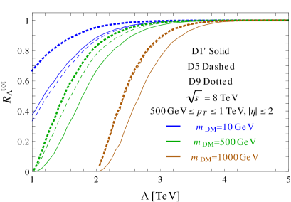
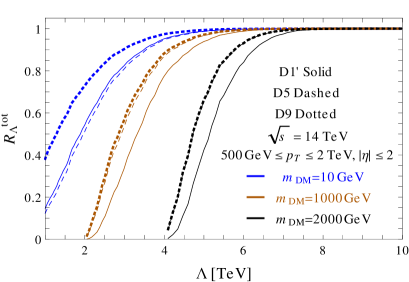
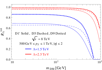
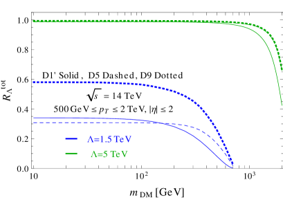
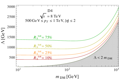
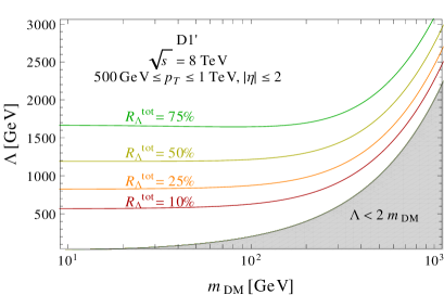
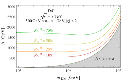
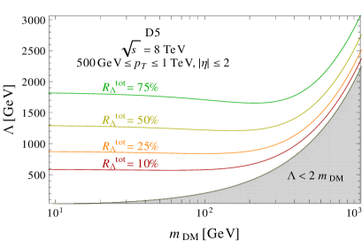
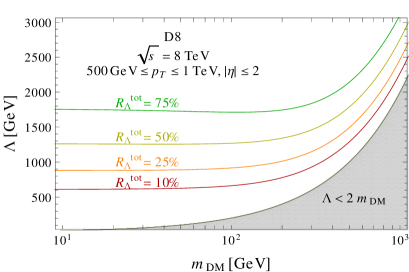
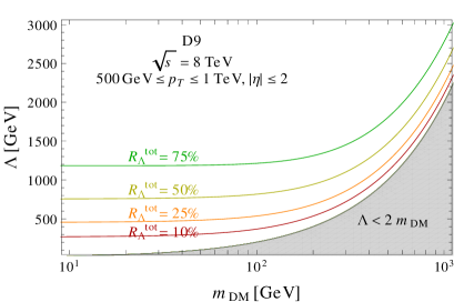
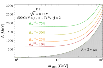
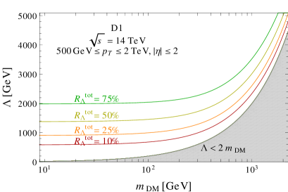
We first study the behavior of the ratio RΛtotsuperscriptsubscript𝑅ΛtotR_{\Lambda}^{\rm tot}, as a function of ΛΛ\Lambda and mDMsubscript𝑚DMm_{\rm DM} The results are shown in Fig. 1. We show only results for representative operators D1,D5,D9𝐷superscript1𝐷5𝐷9D1^{\prime},D5,D9. This ratio RΛtotsuperscriptsubscript𝑅ΛtotR_{\Lambda}^{\rm tot} gets closer to unity for large values of ΛΛ\Lambda, as in this case the effect of the cutoff becomes negligible. The ratio drops for large mDMsubscript𝑚DMm_{\rm DM} because the momentum transfer increases in this regime. This confirms our precedent analysis of Ref. [29], that the EFT works better for large ΛΛ\Lambda and small mDMsubscript𝑚DMm_{\rm DM}. Notice also that, going from s=8TeV𝑠8TeV\sqrt{s}=8{\rm TeV} to s=14TeV𝑠14TeV\sqrt{s}=14{\rm TeV}, the results scale almost linearly with the energy, so for the same value of the ratio mDM/Λsubscript𝑚DMΛm_{\rm DM}/\Lambda one obtains nearly the same RΛtotsuperscriptsubscript𝑅ΛtotR_{\Lambda}^{\rm tot}.

Refer to caption
Refer to caption
Refer to caption
Refer to caption
Figure 1: The ratio RΛtotsuperscriptsubscript𝑅ΛtotR_{\Lambda}^{\rm tot} defined in Eq. (2.18) for operators D1𝐷superscript1D1^{\prime} (solid lines), D5𝐷5D5 (dashed lines) and D9𝐷9D9 (dotted lines) as a function of ΛΛ\Lambda and mDMsubscript𝑚DMm_{\rm DM}, for s=8𝑠8\sqrt{s}=8 TeV (left panel) and 141414 TeV (right panel).
Refer to caption
Refer to caption
Refer to caption
Refer to caption
Refer to caption
Refer to caption
Refer to caption
Refer to caption
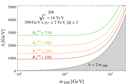
Figure 2: Contours for the ratio RΛtotsuperscriptsubscript𝑅ΛtotR_{\Lambda}^{\rm tot}, defined in Eq. (2.18), on the plane (mDM,Λ)subscript𝑚DMΛ(m_{\rm DM},\Lambda), for the different operators. We set s=8TeV,|η|2formulae-sequence𝑠8TeV𝜂2\sqrt{s}=8{\rm TeV},|\eta|\leq 2 and 500GeV<pT<1TeV500GeVsubscript𝑝T1TeV500{\rm\,GeV}<p_{\rm T}<1{\rm TeV}.
Refer to caption
Refer to caption
Refer to caption
Refer to caption
Refer to caption
Refer to caption
Refer to caption
Refer to caption
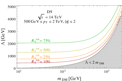
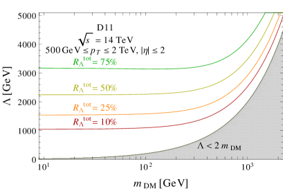
Figure 3: Contours for the ratio RΛtotsuperscriptsubscript𝑅ΛtotR_{\Lambda}^{\rm tot}, defined in Eq. (2.18), on the plane (mDM,Λ)subscript𝑚DMΛ(m_{\rm DM},\Lambda), for the different operators. We set s=14TeV,|η|2formulae-sequence𝑠14TeV𝜂2\sqrt{s}=14{\rm TeV},|\eta|\leq 2 and 500GeV<pT<2TeV500GeVsubscript𝑝T2TeV500{\rm\,GeV}<p_{\rm T}<2{\rm TeV}.

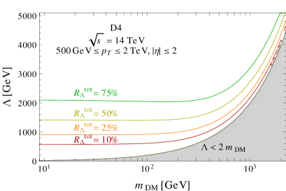
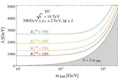
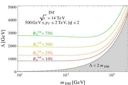
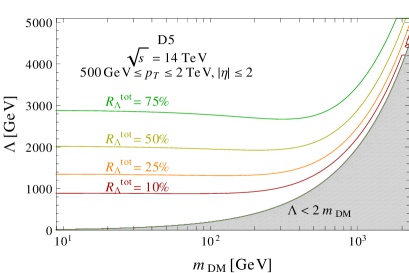
Next, we turn to study the contours of constant values of the quantity RΛtotsuperscriptsubscript𝑅ΛtotR_{\Lambda}^{\rm tot}, in the plane (mDM,Λ)subscript𝑚DMΛ(m_{\rm DM},\Lambda). These contour curves for the different operators are shown in Fig. 2 for s=8𝑠8\sqrt{s}=8 TeV and in Fig. 3 for s=14𝑠14\sqrt{s}=14 TeV. The requirement that at least 50% of the events occur with momentum transfer below the cutoff scale ΛΛ\Lambda requires such a cutoff scale to be above 1TeVsimilar-toabsent1TeV\sim 1{\rm TeV} for s=8TeV𝑠8TeV\sqrt{s}=8\,{\rm TeV}, or above 2TeVsimilar-toabsent2TeV\sim 2{\rm TeV} for s=14TeV𝑠14TeV\sqrt{s}=14\,{\rm TeV}. Note also that the contours for D1𝐷1D1D4𝐷4D4 differ by the corresponding contours for D1𝐷superscript1D1^{\prime}D4𝐷superscript4D4^{\prime} by 𝒪(1)𝒪1{\cal O}(1) factors, due to the different weighting of the quarks’ PDFs. On the other hand, the experimental bounds on the scale of the operators D1𝐷1D1D4𝐷4D4 are much lower (of the order of tens of GeV), as such operators experience an additional suppression of mq/Λsubscript𝑚𝑞Λm_{q}/\Lambda. This means that the bounds on D1𝐷1D1D4𝐷4D4 are not reliable from the point of view of EFT validity.

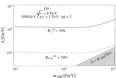
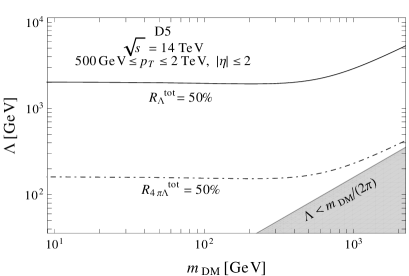
We stress once again that the precise definition of a cutoff scale for an EFT is only possible when the details of the UV completion are known. The most conservative regime is when the couplings of the UV theory reach their maximal values allowed by perturbativity. In such a situation, the requirement on the momentum transfer becomes Qtr<4πΛsubscript𝑄tr4𝜋ΛQ_{\rm tr}<4\pi\Lambda. We show the effect of varying the cutoff scale in Fig. 4, for the representative contour RΛtot=50%superscriptsubscript𝑅Λtotpercent50R_{\Lambda}^{\rm tot}=50\% of D5. As it should be clear, the variation of the cutoff scale is equivalent to a change of the unknown couplings of the UV theory. All the operators have very similar results, as the contours scale linearly with the cutoff. As a comparison, we show as a shaded area the region Λ>mDM/(2π)Λsubscript𝑚DM2𝜋\Lambda>m_{\rm DM}/(2\pi) often used as a benchmark for the validity of the EFT (see Eq. (1.4)). The 50% contour is above such a region, meaning that the parameter space regions of validity of the effective operator approach is smaller than commonly considered.
Refer to caption
Refer to caption
Figure 4: 50% contours for the ratio RΛtotsuperscriptsubscript𝑅ΛtotR_{\Lambda}^{\rm tot} for the operator D5𝐷5D5, varying the cutoff Qtr<Λsubscript𝑄trΛQ_{\rm tr}<\Lambda (solid line) and Qtr<4πΛsubscript𝑄tr4𝜋ΛQ_{\rm tr}<4\pi\Lambda (dot-dashed line). We have also shown the region corresponding to Λ<mDM/(2π)Λsubscript𝑚DM2𝜋\Lambda<m_{\rm DM}/(2\pi) (gray shaded area), often used as a benchmark for the validity of the EFT. We set s=8𝑠8\sqrt{s}=8 TeV (left panel) and s=14𝑠14\sqrt{s}=14 TeV (right panel).

To close this section let us comment on another question one may ask: what is the difference between interpreting data with an effective operator and with its simplest UV completion? This question has already been addressed in Ref. [29] for the operator D1𝐷superscript1D1^{\prime}, by studying the ratio of the cross sections obtained with the UV theory and with the effective operator. For each of the operators in Table 1 one can write a simple UV-complete Lagrangian, see e.g. Eqs. (2.1)-(2.2). The very same analysis can be repeated for all the other operators and we checked that the same qualitative conclusions can be drawn. In particular, if ΛΛ\Lambda is not larger than a few TeV, interpreting the experimental data in terms of EFT or in terms of a simplified model with a mediator can make a significant difference.

3 Comparison with MonteCarlo Simulations

In order to perform an alternative check of our analytical results and to be able to compare to the experimental limits as close as possible, we present in this section the results of numerical event simulations.

3.1 Simulation and analysis description

We made use of MadGraph 5[38] to simulate pp𝑝𝑝pp collisions at s=8𝑠8\sqrt{s}=8 TeV and s=14𝑠14\sqrt{s}=14 TeV. Both PDF sets CTEQ6L1 and MSTW2008LO (discussed in Ref. [39]) are employed. The PDF choice affects the cross section, but only minimally the acceptance. Hence, the change in contours of RΛtotsuperscriptsubscript𝑅ΛtotR_{\Lambda}^{\rm tot} is negligible. Since MSTW2008LO is used for the analytical calculations, this set is also used where direct comparisons between simulation and calculation are shown. For the comparison to the experimental results, CTEQ6L1 is used instead. Only u,d,c,s𝑢𝑑𝑐𝑠u,d,c,s quarks were considered, both in the initial and in the final state.

According to the event kinematics we have evaluated whether or not the conditions of validity discussed in Section 2 are fulfilled. Specifically, we have checked if Eqs. (1.3) and (1.4) are fulfilled, that is, if the following condition is satisfied

Λ>Qtrgqgχ>2mDMgqgχ.Λsubscript𝑄trsubscript𝑔𝑞subscript𝑔𝜒2subscript𝑚DMsubscript𝑔𝑞subscript𝑔𝜒\Lambda>\frac{Q_{\rm tr}}{\sqrt{g_{q}g_{\chi}}}>2\frac{m_{\rm DM}}{\sqrt{g_{q}g_{\chi}}}\,. (3.1)

Samples of 20000 events were simulated for each operator, scanning DM mass values of 10, 50, 80, 100, 400, 600, 800 and 1000 GeV and cutoff scales of 250, 500, 1000, 1500, 2000, 2500 and 3000 GeV in the case of s=8𝑠8\sqrt{s}=8 TeV collisions. When increasing the collision energy to s=14𝑠14\sqrt{s}=14 TeV, the DM mass of 2000 GeV and cutoff scales of 4000 and 5000 GeV were added.

From the simulated samples the fraction of events fulfilling Λ>Qtr/gqgχΛsubscript𝑄trsubscript𝑔𝑞subscript𝑔𝜒\Lambda>Q_{\rm tr}/\sqrt{g_{q}g_{\chi}} for each pair of DM mass and cutoff scale can be evaluated, if one assumes a certain value for the couplings gχgqsubscript𝑔𝜒subscript𝑔𝑞\sqrt{g_{\chi}g_{q}} connecting the cutoff scale ΛΛ\Lambda and the mediator mass M𝑀M via Λ=M/gqgχΛ𝑀subscript𝑔𝑞subscript𝑔𝜒\Lambda=M/\sqrt{g_{q}g_{\chi}}. As above, gqgχsubscript𝑔𝑞subscript𝑔𝜒g_{q}g_{\chi} was assumed to be 1.

Refer to caption
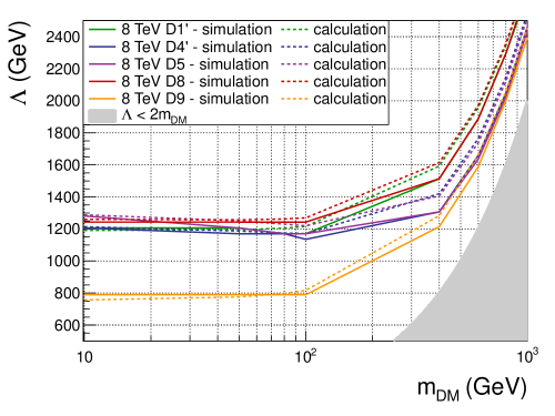
Figure 5: Comparison of the contour RΛtot=50%superscriptsubscript𝑅Λtotpercent50R_{\Lambda}^{\rm tot}=50\% for the analytical calculation (dashed line) and the simulation (solid line) for the different operators D1𝐷superscript1D1^{\prime}, D4𝐷superscript4D4^{\prime}, D5𝐷5D5, D8𝐷8D8 and D9𝐷9D9. The results agree within less than 7 %.

3.2 Results

In order to confirm that analytical and numerical results are in agreement, Figure 5 shows a comparison for the operators D1𝐷superscript1D1^{\prime}, D4𝐷superscript4D4^{\prime}, D5𝐷5D5, D8𝐷8D8 and D9𝐷9D9. The results were obtained for the scenario of one radiated gluon jet above 500 GeV within |η|<2𝜂2|\eta|<2. The contours of RΛtot=50%superscriptsubscript𝑅Λtotpercent50R_{\Lambda}^{\rm tot}=50\% from analytical and numerical evaluation agree within less than 7 %. The remaining differences could be due to the upper jet pTsubscript𝑝Tp_{\rm T} cut not imposed during event simulation but needed for the analytical calculation, and the details of the fitting procedures.
Refer to caption
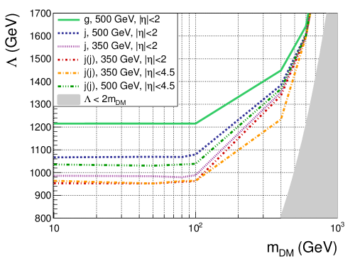
Figure 6: The changes of the contour of RΛtot=50%superscriptsubscript𝑅Λtotpercent50R_{\Lambda}^{\rm tot}=50\% are shown for several variations from the analytically calculated scenario to a scenario close to the cuts used in the ATLAS monojet analysis exemplarily for the operator D5𝐷5D5 at s=8𝑠8\sqrt{s}=8 TeV. In the legend, “g” means only gluon radiation, “j” stands for either quark- or gluon-initiated jets, “j(j)” means a second jet is allowed.

Next, we vary the kinematical constraints step by step from the scenario considered in the analytical calculations, namely one radiated gluon jet above 500 GeV within |η|<2𝜂2|\eta|<2, to a scenario closest to the analysis cuts applied in the ATLAS monojet analysis [12]. More specifically, the leading jet is allowed to come from either a gluon or a quark being radiated, the leading jet pTsubscript𝑝Tp_{\rm T} cut is changed from 500 GeV to 350 GeV, a second jet is allowed and its range in η𝜂\eta is enlarged to |η|<4.5𝜂4.5|\eta|<4.5. No further cuts are applied at simulation level.

The effect of the variation of the cuts can be seen in Figure 6. Allowing not only for a gluon jet but also taking into account the possibility of a quark jet changes the RΛtotsuperscriptsubscript𝑅ΛtotR_{\Lambda}^{\rm tot} contours appreciably. The change from lowering the pTsubscript𝑝Tp_{\rm T} of the leading jet has a smaller effect. Allowing for a second jet and enhancing its rapidity range barely changes the RΛtotsuperscriptsubscript𝑅ΛtotR_{\Lambda}^{\rm tot} contour, especially at large mDMsubscript𝑚DMm_{\rm DM} values.

If the collision energy is augmented to s=14𝑠14\sqrt{s}=14 TeV, all the RΛtotsuperscriptsubscript𝑅ΛtotR_{\Lambda}^{\rm tot} contours increase. As seen for s=8𝑠8\sqrt{s}=8 TeV, moving to the scenario closer to the experimental analysis leads to contours that are at most 30%similar-toabsentpercent30\sim 30\% lower in ΛΛ\Lambda.

After having extracted RΛtotsuperscriptsubscript𝑅ΛtotR_{\Lambda}^{\rm tot} for each WIMP and mediator mass, a curve can be fitted through the points obtained in the plane of RΛtotsuperscriptsubscript𝑅ΛtotR_{\Lambda}^{\rm tot} and ΛΛ\Lambda. The following functional form is used for this purpose

RΛtot=[1ea(Λ2mDMb)c][1ed(Λ+2mDMb)e].superscriptsubscript𝑅Λtotdelimited-[]1superscript𝑒𝑎superscriptΛ2subscript𝑚DM𝑏𝑐delimited-[]1superscript𝑒𝑑superscriptΛ2subscript𝑚DM𝑏𝑒R_{\Lambda}^{\rm tot}=\left[1-e^{-a\left(\frac{\Lambda-2m_{\rm DM}}{b}\right)^{c}}\right]\left[1-e^{-d\left(\frac{\Lambda+2m_{\rm DM}}{b}\right)^{e}}\right]\,. (3.2)

Further, the parameters are fitted for each DM mass separately. From these fits, the points denoting a cutoff scale where RΛtotsuperscriptsubscript𝑅ΛtotR_{\Lambda}^{\rm tot} equals e.g. 50% can be extracted for each DM mass, and the lines of constant RΛtotsuperscriptsubscript𝑅ΛtotR_{\Lambda}^{\rm tot} can be plotted in the usual limit-setting plane ΛΛ\Lambda vs. mDMsubscript𝑚DMm_{\rm DM}. Table 2 collects the values of the fitting parameters for all operators except D12-D14, for which no experimental analysis exists.

s=8𝑠8\sqrt{s}=8 TeV s=14𝑠14\sqrt{s}=14 TeV
Operator a b c d e
D1 1.32 787.13 1.39 1.08 1.53
D1’ 1.30 1008.25 1.49 0.77 1.83
D4 1.65 702.93 1.14 0.65 1.75
D4’ 1.51 859.83 1.22 0.48 1.92
D5 1.54 816.83 1.18 0.50 1.85
D8 1.23 964.62 1.50 0.91 1.59
D9 1.43 681.92 1.15 1.02 1.35
D11 1.23 1002.33 1.49 0.82 1.69
Operator a b c d e
D1 0.89 1017.37 1.45 1.28 1.24
D1’ 0.43 909.66 1.59 0.53 1.37
D4 1.23 996.82 1.25 0.80 1.48
D4’ 0.76 982.75 1.33 0.37 1.63
D5 0.78 894.86 1.25 0.39 1.54
D8 0.48 945.09 1.55 0.74 1.24
D9 0.91 891.65 1.21 1.23 1.04
D11 0.68 1250.49 1.58 0.81 1.35
Table 2: Coefficient for the fitting functions for RΛtotsuperscriptsubscript𝑅ΛtotR_{\Lambda}^{\rm tot} in Eq. (3.2), in the cases s=𝑠absent\sqrt{s}= 8 and 14 TeV. The fitting functions describe processes where quarks and/or gluons are radiated, the final state contains 1 or 2 jets, where the leading jet has minimum pTsubscript𝑝Tp_{\rm T} of 350 GeV while the second jet is allowed to be within |η|<4.5𝜂4.5|\eta|<4.5. See text for further details.

4 Implications of the limited validity of EFT in DM searches at LHC

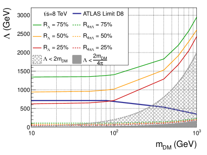
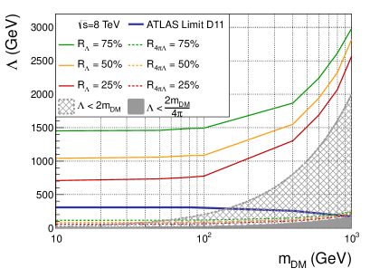
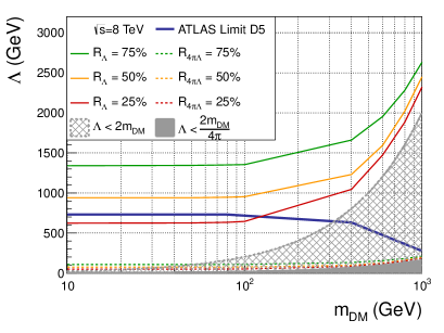
Figure 7 shows the experimental limits obtained from the ATLAS monojet analysis [12] in the plane (Λ(\Lambda, mDMsubscript𝑚DMm_{\rm DM}), for the opearators D5, D8 and D11. The contours of RΛtotsuperscriptsubscript𝑅ΛtotR_{\Lambda}^{\rm tot} for 25%, 50% and 75% are superimposed. The experimental limits are placed in a region where about 30% of the events can be expected to fulfill the EFT conditions - the exact number depends on the operator considered. Especially the limit on the gluon operator D11𝐷11D11 seems questionnable. For comparison, dashed lines show the contours of RΛtotsuperscriptsubscript𝑅ΛtotR_{\Lambda}^{\rm tot} for the extreme case of couplings gqgχ=4πsubscript𝑔𝑞subscript𝑔𝜒4𝜋\sqrt{g_{q}g_{\chi}}=4\pi, presenting the limiting case for which the theory is still considered perturbative.
Refer to caption
Refer to caption
Refer to caption
Figure 7: 25%, 50% and 75% contours for the ratio RΛtotsuperscriptsubscript𝑅ΛtotR_{\Lambda}^{\rm tot}, compared to the experimental limits from ATLAS [12] (blue line). Also indicated are the contours of RΛtotsuperscriptsubscript𝑅ΛtotR_{\Lambda}^{\rm tot} in the extreme case when setting the couplings gqgχ=4πsubscript𝑔𝑞subscript𝑔𝜒4𝜋\sqrt{g_{q}g_{\chi}}=4\pi (dashed lines). Results are shown for different operators: D5 (upper left panel), D8 (upper right panel) and D11 (lower panel).

Unfortuntately, there is no possibility to measure Qtrsubscript𝑄trQ_{\rm tr} in data, on an event-by-event basis. So the information on what is the fraction of the events to cut out comes from analytical computations or a numerical simulation, as we explained in this paper. To assess the impact of the limited validity of the EFT on the current collider bounds, we adopt the procedure that relies on the assumption that the pTsubscript𝑝Tp_{\rm T} (or MET) distributions with the Qtrsubscript𝑄trQ_{\rm tr} cut are simply a rescaling of those without the cut. A more refined study should account for possible kinematic shape changes with the jet transverse momentum and/or missing energy and DM mass222Preliminary studies indicate that the method adopted in this paper is quite reasonable for cuts with Qtr<750subscript𝑄tr750Q_{\rm tr}<750 GeV or weaker [40]..

Very naively, neglecting the statistical and systematical uncertainties, the number of signal events in a given EFT model has to be less than the experimental observation, Nsignal(Λ,mDM)<Nexptsubscript𝑁signalΛsubscript𝑚DMsubscript𝑁exptN_{\rm signal}(\Lambda,m_{\rm DM})<N_{\rm expt}. The cross section due to an operator of mass dimension d𝑑d scale like Λ2(d4)superscriptΛ2𝑑4\Lambda^{-2(d-4)}, so Nsignal(Λ,mDM)=Λ2(d4)N~signal(mDM)subscript𝑁signalΛsubscript𝑚DMsuperscriptΛ2𝑑4subscript~𝑁signalsubscript𝑚DMN_{\rm signal}(\Lambda,m_{\rm DM})=\Lambda^{-2(d-4)}\tilde{N}_{\rm signal}(m_{\rm DM}), and the experimental lower bound in the scale of the operator becomes

Λ>[N~signal(mDM)/Nexp]1/[2(d4)]Λexpt..Λsuperscriptdelimited-[]subscript~𝑁signalsubscript𝑚DMsubscript𝑁exp1delimited-[]2𝑑4subscriptΛexpt\Lambda>\left[\tilde{N}_{\rm signal}(m_{\rm DM})/N_{\rm exp}\right]^{1/[2(d-4)]}\equiv\Lambda_{\rm expt.}\,. (4.1)

Now, if we do not consider any information about the shapes of the pTsubscript𝑝Tp_{\rm T} or MET distributions, the experimental bound only comes from the total number of events passing given cuts. The fact that a fraction of the events involve a transfer momentum exceeding the cutoff scale of the EFT means that the number of signal events for placing a limit gets reduced by a factor RΛtotsuperscriptsubscript𝑅ΛtotR_{\Lambda}^{\rm tot}. Therefore, actually Nsignal(Λ,mDM)RΛtot(mDM)Nsignal(Λ,mDM)subscript𝑁signalΛsubscript𝑚DMsuperscriptsubscript𝑅Λtotsubscript𝑚DMsubscript𝑁signalΛsubscript𝑚DMN_{\rm signal}(\Lambda,m_{\rm DM})\to R_{\Lambda}^{\rm tot}(m_{\rm DM})N_{\rm signal}(\Lambda,m_{\rm DM}), so the new limit is found by solving the implicit equation

Λ>[RΛtot(mDM)]1/2[(d4)][Nsignal(mDM)/Nexp]1/[2(d4)]=[RΛtot(mDM)]1/[2(d4)]ΛexptΛsuperscriptdelimited-[]superscriptsubscript𝑅Λtotsubscript𝑚DM12delimited-[]𝑑4superscriptdelimited-[]subscript𝑁signalsubscript𝑚DMsubscript𝑁exp1delimited-[]2𝑑4superscriptdelimited-[]superscriptsubscript𝑅Λtotsubscript𝑚DM1delimited-[]2𝑑4subscriptΛexpt\Lambda>[R_{\Lambda}^{\rm tot}(m_{\rm DM})]^{1/2[(d-4)]}[N_{\rm signal}(m_{\rm DM})/N_{\rm exp}]^{1/[2(d-4)]}=[R_{\Lambda}^{\rm tot}(m_{\rm DM})]^{1/[2(d-4)]}\Lambda_{\rm expt} (4.2)

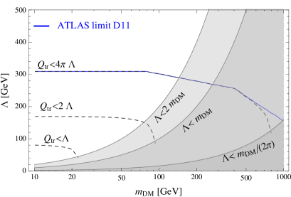
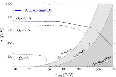
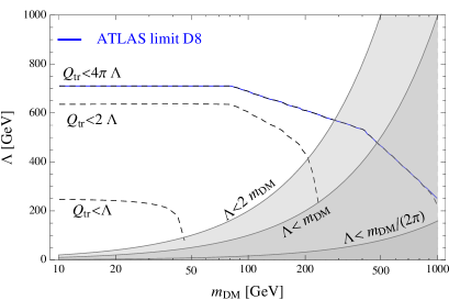
and it turns out to be weaker than ΛexptsubscriptΛexpt\Lambda_{\rm expt}. In Fig. 8 we show the new limits for the dim-6 operators D5, D8 and the dim-7 operator D11, for the conditions Qtr<Λ,2Λ,4πΛsubscript𝑄trΛ2Λ4𝜋ΛQ_{\rm tr}<\Lambda,2\Lambda,4\pi\Lambda, corresponding different choices of the UV couplings: gqgχ=1,2,4πsubscript𝑔𝑞subscript𝑔𝜒124𝜋\sqrt{g_{q}g_{\chi}}=1,2,4\pi, respectively. The curves are obtained solving Eq. 4.2 with RΛtot,R2Λtot,R4πΛtotsuperscriptsubscript𝑅Λtotsuperscriptsubscript𝑅2Λtotsuperscriptsubscript𝑅4𝜋ΛtotR_{\Lambda}^{\rm tot},R_{2\Lambda}^{\rm tot},R_{4\pi\Lambda}^{\rm tot} respectively. The ATLAS bound reported is the 90%CL observed limit. The functions RΛtotsuperscriptsubscript𝑅ΛtotR_{\Lambda}^{\rm tot} used are taken from the fitting functions described in Table 2, which include both quark and gluon jets, and the same cuts as the “Signal Region 3” used by ATLAS. As expected, the weaker is the condition on Qtrsubscript𝑄trQ_{\rm tr}, the more the new limits approach the ATLAS bound. In the case of extreme couplings gqgχ=4πsubscript𝑔𝑞subscript𝑔𝜒4𝜋\sqrt{g_{q}g_{\chi}}=4\pi, the condition on the momentum transfer is very conservative Qtr<4πΛsubscript𝑄tr4𝜋ΛQ_{\rm tr}<4\pi\Lambda. For D5 and D8, the new limit is indisinguishable from the ATLAS one, meaning that the experimental results are safe from the EFT point of view, in this limiting situation. For D11, even for extreme values of the couplings, the bound at large DM masses must be corrected. In general, for couplings of order one, the limits which are safe from the EFT point of view are appreciably weaker than those reported. We encourage the experimental collaborations to take this point into account when publishing their limits.
Refer to caption
Refer to caption
Refer to caption
Figure 8: The experimental limits by ATLAS [12] on the suppression scale ΛΛ\Lambda are shown as solid blue lines. The updated limits taking into account EFT validity are shown as dashed black lines, for Qtr<Λ,2Λ,4πΛsubscript𝑄trΛ2Λ4𝜋ΛQ_{\rm tr}<\Lambda,2\Lambda,4\pi\Lambda, corresponding to different choices of the UV couplings: gqgχ=1,2,4πsubscript𝑔𝑞subscript𝑔𝜒124𝜋\sqrt{g_{q}g_{\chi}}=1,2,4\pi, respectively. The corresponding kinematical constraints (Eq. (3.1)) are denoted by gray bands. The different plots refer to different operators: D5 (upper left panel), D8 (upper right panel) and D11 (lower panel).

5 Conclusions

The search for DM is one of the main targets of LHC analyses. In this paper we have continued our previous investigation to assess the validity of the EFT commonly used in interpreting such searches. Following Ref. [29], we have studied the quantity RΛtotsuperscriptsubscript𝑅ΛtotR_{\Lambda}^{\rm tot} (see Eq.( 2.18), which quantifies the error made when using effective operators to describe processes with very high momentum transfer. Our criterion indicates up to what cutoff energy scale the effective description is valid, depending on the DM mass and couplings. We have performed the analysis for the full list of EFT operators, connecting fermion DM particles and quarks or gluons, used by the ATLAS and CMS collaborations and originated from the exchange of heavy mediators in the s𝑠s-channel. We have also extended our analysis to the case of s=𝑠absent\sqrt{s}= 14 TeV. Furthermore, we have validated our analytical results by performing numerical event simulations which reproduce the experimental situation in the closest possible way. Our results indicate that the range of validity of the EFT is significantly limited in the parameter space (Λ,mDM)Λsubscript𝑚DM(\Lambda,m_{\rm DM}). While our findings are valid for the s𝑠s-channel, a similar analysis is under way for the t𝑡t-channel [41] where similar results are obtained.

Does it mean that the EFT is not the best tool to interpret the current LHC data of DM searches? The answer is yes and no. On the negative side, our results clearly cry out for an overcoming of the EFT, most possibly through identifying a handful of classes of models (able to reproduce the EFT operators in the heavy mediator limit); this would allow a consistent analysis of the current and future LHC data by consistently taking into account the role played by the mediator. On the positive side, keep working with the EFT allows to avoid the overwhelming model-dependence generated by the many DM models proposed so far. Nonetheless, as we have shown in section 4, the price to pay is a deterioration of the limits presented so far.

Acknowledgments

We thank A. Brennan, C. Doglioni, G. Iacobucci, T. Jacques, S. Schramm and S. Vallecorsa for many interesting conversations. ADS acknowledges partial support from the European Union FP7 ITN INVISIBLES (Marie Curie Actions, PITN-GA-2011-289442). JG acknowledges partial support from UNIGE and SNF grant 200020-144493, “High-Energy Hadron Interactions: ATLAS at the CERN LHC”.

Appendix A Three-body Cross Sections

A.1 Generalities

In this Appendix we show the details of the calculations of the tree-level cross sections for the hard scattering process f(p1)+f¯(p2)χ(p3)+χ(p4)+g(k)𝑓subscript𝑝1¯𝑓subscript𝑝2𝜒subscript𝑝3𝜒subscript𝑝4𝑔𝑘f(p_{1})+\bar{f}(p_{2})\to\chi(p_{3})+\chi(p_{4})+g(k), where f𝑓f is either a quark (operators D1-D10) or a gluon (D11-D14), and the final gluon is emitted from the initial state.

The differential cross section is generically given by

dσ^=||2¯4(p1p2)dΦ3,𝑑^𝜎¯superscript24subscript𝑝1subscript𝑝2dsubscriptΦ3d\hat{\sigma}=\frac{\sum\overline{|{\cal M}|^{2}}}{4(p_{1}\cdot p_{2})}\textrm{d}\Phi_{3}\,, (A.1)

where the three-body phase space is

dΦ3=(2π)4δ(4)(p1+p2p3p4k)dp3(2π)32p30dp4(2π)32p40dk(2π)32k0.dsubscriptΦ3superscript2𝜋4superscript𝛿4subscript𝑝1subscript𝑝2subscript𝑝3subscript𝑝4𝑘dsubscriptp3superscript2𝜋32superscriptsubscript𝑝30dsubscriptp4superscript2𝜋32superscriptsubscript𝑝40dksuperscript2𝜋32superscript𝑘0\textrm{d}\Phi_{3}=(2\pi)^{4}\delta^{(4)}(p_{1}+p_{2}-p_{3}-p_{4}-k)\frac{{\rm d}\textbf{p}_{3}}{(2\pi)^{3}2p_{3}^{0}}\frac{{\rm d}\textbf{p}_{4}}{(2\pi)^{3}2p_{4}^{0}}\frac{{\rm d}\textbf{k}}{(2\pi)^{3}2k^{0}}\,. (A.2)

A.2 Matrix Elements

In the limit of massless light quarks, they have definite helicity and it makes no difference for the cross sections whether there is q𝑞q or γ5qsuperscript𝛾5𝑞\gamma^{5}q in the operator. Therefore the following identifications between pairs of operators hold:

D1D3,D2D4,D5D7,D6D8,D9D10,𝐷superscript1𝐷superscript3𝐷superscript2𝐷superscript4𝐷5𝐷7𝐷6𝐷8𝐷9𝐷10D1^{\prime}\leftrightarrow D3^{\prime},\qquad D2^{\prime}\leftrightarrow D4^{\prime},\qquad D5\leftrightarrow D7,\qquad D6\leftrightarrow D8,\qquad D9\leftrightarrow D10\,, (A.3)

while the “primed” and “unprimed” operators are related as in Eq. (2.16). For definiteness, we choose to work with D1,D4,D5,D8,D9𝐷superscript1𝐷superscript4𝐷5𝐷8𝐷9D1^{\prime},D4^{\prime},D5,D8,D9 and D11D14𝐷11𝐷14D11-D14.

The amplitudes are given by

D1subscript𝐷superscript1\displaystyle{\cal M}_{D1^{\prime}} =\displaystyle= igs1Λ2ϵμa(k)[v¯(p2)(p1k)γμTau(p1)(p1k)2v¯(p2)γμTa(p2k)u(p1)(p2k)2]u¯(p3)v(p4),𝑖subscript𝑔𝑠1superscriptΛ2superscriptsubscriptitalic-ϵ𝜇absent𝑎𝑘delimited-[]¯𝑣subscript𝑝2subscriptcancel𝑝1cancel𝑘superscript𝛾𝜇superscript𝑇𝑎𝑢subscript𝑝1superscriptsubscript𝑝1𝑘2¯𝑣subscript𝑝2superscript𝛾𝜇superscript𝑇𝑎subscriptcancel𝑝2cancel𝑘𝑢subscript𝑝1superscriptsubscript𝑝2𝑘2¯𝑢subscript𝑝3𝑣subscript𝑝4\displaystyle-ig_{s}\frac{1}{\Lambda^{2}}\epsilon_{\mu}^{*a}(k)\left[\frac{\bar{v}(p_{2})({\cancel{p}_{1}}-\cancel{k})\gamma^{\mu}T^{a}u(p_{1})}{(p_{1}-k)^{2}}-\frac{\bar{v}(p_{2})\gamma^{\mu}T^{a}({\cancel{p}_{2}}-\cancel{k})u(p_{1})}{(p_{2}-k)^{2}}\right]\bar{u}(p_{3})v(p_{4})\,, (A.4)
D4subscript𝐷superscript4\displaystyle{\cal M}_{D4^{\prime}} =\displaystyle= igs1Λ2ϵμa(k)[v¯(p2)γ5(p1k)γμTau(p1)(p1k)2v¯(p2)γμTa(p2k)γ5u(p1)(p2k)2]𝑖subscript𝑔𝑠1superscriptΛ2superscriptsubscriptitalic-ϵ𝜇absent𝑎𝑘delimited-[]¯𝑣subscript𝑝2superscript𝛾5subscriptcancel𝑝1cancel𝑘superscript𝛾𝜇superscript𝑇𝑎𝑢subscript𝑝1superscriptsubscript𝑝1𝑘2¯𝑣subscript𝑝2superscript𝛾𝜇superscript𝑇𝑎subscriptcancel𝑝2cancel𝑘superscript𝛾5𝑢subscript𝑝1superscriptsubscript𝑝2𝑘2\displaystyle-ig_{s}\frac{1}{\Lambda^{2}}\epsilon_{\mu}^{*a}(k)\left[\frac{\bar{v}(p_{2})\gamma^{5}({\cancel{p}_{1}}-\cancel{k})\gamma^{\mu}T^{a}u(p_{1})}{(p_{1}-k)^{2}}-\frac{\bar{v}(p_{2})\gamma^{\mu}T^{a}({\cancel{p}_{2}}-\cancel{k})\gamma^{5}u(p_{1})}{(p_{2}-k)^{2}}\right] (A.5)
×u¯(p3)γ5v(p4),absent¯𝑢subscript𝑝3superscript𝛾5𝑣subscript𝑝4\displaystyle\times\bar{u}(p_{3})\gamma^{5}v(p_{4})\,,
D5subscript𝐷5\displaystyle{\cal M}_{D5} =\displaystyle= igsgνρΛ2ϵμa(k)[v¯(p2)γν(p1k)γμTau(p1)(p1k)2v¯(p2)γμTa(p2k)γνu(p1)(p2k)2]𝑖subscript𝑔𝑠subscript𝑔𝜈𝜌superscriptΛ2superscriptsubscriptitalic-ϵ𝜇absent𝑎𝑘delimited-[]¯𝑣subscript𝑝2superscript𝛾𝜈subscriptcancel𝑝1cancel𝑘superscript𝛾𝜇superscript𝑇𝑎𝑢subscript𝑝1superscriptsubscript𝑝1𝑘2¯𝑣subscript𝑝2superscript𝛾𝜇superscript𝑇𝑎subscriptcancel𝑝2cancel𝑘superscript𝛾𝜈𝑢subscript𝑝1superscriptsubscript𝑝2𝑘2\displaystyle-ig_{s}\frac{g_{\nu\rho}}{\Lambda^{2}}\epsilon_{\mu}^{*a}(k)\left[\frac{\bar{v}(p_{2})\gamma^{\nu}({\cancel{p}_{1}}-\cancel{k})\gamma^{\mu}T^{a}u(p_{1})}{(p_{1}-k)^{2}}-\frac{\bar{v}(p_{2})\gamma^{\mu}T^{a}({\cancel{p}_{2}}-\cancel{k})\gamma^{\nu}u(p_{1})}{(p_{2}-k)^{2}}\right] (A.6)
×u¯(p3)γρv(p4),absent¯𝑢subscript𝑝3superscript𝛾𝜌𝑣subscript𝑝4\displaystyle\times\bar{u}(p_{3})\gamma^{\rho}v(p_{4})\,,
D8subscript𝐷8\displaystyle{\cal M}_{D8} =\displaystyle= igsgνρΛ2ϵμa(k)[v¯(p2)γνγ5(p1k)γμTau(p1)(p1k)2v¯(p2)γμTa(p2k)γνγ5u(p1)(p2k)2]𝑖subscript𝑔𝑠subscript𝑔𝜈𝜌superscriptΛ2superscriptsubscriptitalic-ϵ𝜇absent𝑎𝑘delimited-[]¯𝑣subscript𝑝2superscript𝛾𝜈superscript𝛾5subscriptcancel𝑝1cancel𝑘superscript𝛾𝜇superscript𝑇𝑎𝑢subscript𝑝1superscriptsubscript𝑝1𝑘2¯𝑣subscript𝑝2superscript𝛾𝜇superscript𝑇𝑎subscriptcancel𝑝2cancel𝑘superscript𝛾𝜈superscript𝛾5𝑢subscript𝑝1superscriptsubscript𝑝2𝑘2\displaystyle-ig_{s}\frac{g_{\nu\rho}}{\Lambda^{2}}\epsilon_{\mu}^{*a}(k)\left[\frac{\bar{v}(p_{2})\gamma^{\nu}\gamma^{5}({\cancel{p}_{1}}-\cancel{k})\gamma^{\mu}T^{a}u(p_{1})}{(p_{1}-k)^{2}}-\frac{\bar{v}(p_{2})\gamma^{\mu}T^{a}({\cancel{p}_{2}}-\cancel{k})\gamma^{\nu}\gamma^{5}u(p_{1})}{(p_{2}-k)^{2}}\right] (A.7)
×u¯(p3)γργ5v(p4),absent¯𝑢subscript𝑝3superscript𝛾𝜌superscript𝛾5𝑣subscript𝑝4\displaystyle\times\bar{u}(p_{3})\gamma^{\rho}\gamma^{5}v(p_{4})\,,
D9subscript𝐷9\displaystyle{\cal M}_{D9} =\displaystyle= igs16gμρgνσΛ2ϵαa(k)[v¯(p2)σμν(p1k)γαTau(p1)(p1k)2v¯(p2)γαTa(p2k)σμνu(p1)(p2k)2]𝑖subscript𝑔𝑠16subscript𝑔𝜇𝜌subscript𝑔𝜈𝜎superscriptΛ2superscriptsubscriptitalic-ϵ𝛼absent𝑎𝑘delimited-[]¯𝑣subscript𝑝2superscript𝜎𝜇𝜈subscriptcancel𝑝1cancel𝑘superscript𝛾𝛼superscript𝑇𝑎𝑢subscript𝑝1superscriptsubscript𝑝1𝑘2¯𝑣subscript𝑝2superscript𝛾𝛼superscript𝑇𝑎subscriptcancel𝑝2cancel𝑘superscript𝜎𝜇𝜈𝑢subscript𝑝1superscriptsubscript𝑝2𝑘2\displaystyle-i\frac{g_{s}}{16}\frac{g_{\mu\rho}g_{\nu\sigma}}{\Lambda^{2}}\epsilon_{\alpha}^{*a}(k)\left[\frac{\bar{v}(p_{2})\sigma^{\mu\nu}({\cancel{p}_{1}}-\cancel{k})\gamma^{\alpha}T^{a}u(p_{1})}{(p_{1}-k)^{2}}-\frac{\bar{v}(p_{2})\gamma^{\alpha}T^{a}({\cancel{p}_{2}}-\cancel{k})\sigma^{\mu\nu}u(p_{1})}{(p_{2}-k)^{2}}\right] (A.8)
×u¯(p3)σρσv(p4),absent¯𝑢subscript𝑝3superscript𝜎𝜌𝜎𝑣subscript𝑝4\displaystyle\times\bar{u}(p_{3})\sigma^{\rho\sigma}v(p_{4})\,,
D11subscript𝐷11\displaystyle{\cal M}_{D11} =\displaystyle= gs34π1Λ3fabcϵμ(p1)ϵν(p2)ϵρ(k)u¯(p3)v(p4)superscriptsubscript𝑔𝑠34𝜋1superscriptΛ3subscript𝑓𝑎𝑏𝑐subscriptitalic-ϵ𝜇subscript𝑝1subscriptitalic-ϵ𝜈subscript𝑝2superscriptsubscriptitalic-ϵ𝜌𝑘¯𝑢subscript𝑝3𝑣subscript𝑝4\displaystyle\frac{g_{s}^{3}}{4\pi}\frac{1}{\Lambda^{3}}f_{abc}\epsilon_{\mu}(p_{1})\epsilon_{\nu}(p_{2})\epsilon_{\rho}^{*}(k)\bar{u}(p_{3})v(p_{4}) (A.9)
[(gμσ(2p1k)ρ+gρσ(2kp1)μgμρ(k+p1)σ)((p1k)νp2σ(p1k)p2gσν)(p1k)2\displaystyle\left[\frac{(g^{\mu\sigma}(2p_{1}-k)^{\rho}+g^{\rho\sigma}(2k-p_{1})^{\mu}-g^{\mu\rho}(k+p_{1})^{\sigma})((p_{1}-k)^{\nu}p_{2\sigma}-(p_{1}-k)\cdot p_{2}g_{\sigma}^{\nu})}{(p_{1}-k)^{2}}\right.
(gνσ(2p2k)ρ+gρσ(2kp2)νgνρ(k+p2)σ)((p2k)μp1σ(p2k)p1gσμ)(p2k)2superscript𝑔𝜈𝜎superscript2subscript𝑝2𝑘𝜌superscript𝑔𝜌𝜎superscript2𝑘subscript𝑝2𝜈superscript𝑔𝜈𝜌superscript𝑘subscript𝑝2𝜎superscriptsubscript𝑝2𝑘𝜇subscript𝑝1𝜎subscript𝑝2𝑘subscript𝑝1superscriptsubscript𝑔𝜎𝜇superscriptsubscript𝑝2𝑘2\displaystyle-\frac{(g^{\nu\sigma}(2p_{2}-k)^{\rho}+g^{\rho\sigma}(2k-p_{2})^{\nu}-g^{\nu\rho}(k+p_{2})^{\sigma})((p_{2}-k)^{\mu}p_{1\sigma}-(p_{2}-k)\cdot p_{1}g_{\sigma}^{\mu})}{(p_{2}-k)^{2}}
(gμν(p1p2)σ+gνσ(p1+2p2)μgμσ(2p1+p2)ν)((p1+p2)ρkσk(p1+p2)gσρ)(p1+p2)2superscript𝑔𝜇𝜈superscriptsubscript𝑝1subscript𝑝2𝜎superscript𝑔𝜈𝜎superscriptsubscript𝑝12subscript𝑝2𝜇superscript𝑔𝜇𝜎superscript2subscript𝑝1subscript𝑝2𝜈superscriptsubscript𝑝1subscript𝑝2𝜌subscript𝑘𝜎𝑘subscript𝑝1subscript𝑝2superscriptsubscript𝑔𝜎𝜌superscriptsubscript𝑝1subscript𝑝22\displaystyle-\frac{(g^{\mu\nu}(p_{1}-p_{2})^{\sigma}+g^{\nu\sigma}(p_{1}+2p_{2})^{\mu}-g^{\mu\sigma}(2p_{1}+p_{2})^{\nu})((p_{1}+p_{2})^{\rho}k_{\sigma}-k\cdot(p_{1}+p_{2})g_{\sigma}^{\rho})}{(p_{1}+p_{2})^{2}}
+gμν(p1p2)ρ+gνρ(p2+k)μgμρ(k+p1)ν],\displaystyle\left.+g^{\mu\nu}(p_{1}-p_{2})^{\rho}+g^{\nu\rho}(p_{2}+k)^{\mu}-g^{\mu\rho}(k+p_{1})^{\nu}\right]\,,
D12subscript𝐷12\displaystyle{\cal M}_{D12} =\displaystyle= igs34π1Λ3fabcϵμ(p1)ϵν(p2)ϵρ(k)u¯(p3)γ5v(p4)𝑖superscriptsubscript𝑔𝑠34𝜋1superscriptΛ3subscript𝑓𝑎𝑏𝑐subscriptitalic-ϵ𝜇subscript𝑝1subscriptitalic-ϵ𝜈subscript𝑝2superscriptsubscriptitalic-ϵ𝜌𝑘¯𝑢subscript𝑝3superscript𝛾5𝑣subscript𝑝4\displaystyle i\frac{g_{s}^{3}}{4\pi}\frac{1}{\Lambda^{3}}f_{abc}\epsilon_{\mu}(p_{1})\epsilon_{\nu}(p_{2})\epsilon_{\rho}^{*}(k)\bar{u}(p_{3})\gamma^{5}v(p_{4}) (A.10)
[(gμσ(2p1k)ρ+gρσ(2kp1)μgμρ(k+p1)σ)((p1k)νp2σ(p1k)p2gσν)(p1k)2\displaystyle\left[\frac{(g^{\mu\sigma}(2p_{1}-k)^{\rho}+g^{\rho\sigma}(2k-p_{1})^{\mu}-g^{\mu\rho}(k+p_{1})^{\sigma})((p_{1}-k)^{\nu}p_{2\sigma}-(p_{1}-k)\cdot p_{2}g_{\sigma}^{\nu})}{(p_{1}-k)^{2}}\right.
(gνσ(2p2k)ρ+gρσ(2kp2)νgνρ(k+p2)σ)((p2k)μp1σ(p2k)p1gσμ)(p2k)2superscript𝑔𝜈𝜎superscript2subscript𝑝2𝑘𝜌superscript𝑔𝜌𝜎superscript2𝑘subscript𝑝2𝜈superscript𝑔𝜈𝜌superscript𝑘subscript𝑝2𝜎superscriptsubscript𝑝2𝑘𝜇subscript𝑝1𝜎subscript𝑝2𝑘subscript𝑝1superscriptsubscript𝑔𝜎𝜇superscriptsubscript𝑝2𝑘2\displaystyle-\frac{(g^{\nu\sigma}(2p_{2}-k)^{\rho}+g^{\rho\sigma}(2k-p_{2})^{\nu}-g^{\nu\rho}(k+p_{2})^{\sigma})((p_{2}-k)^{\mu}p_{1\sigma}-(p_{2}-k)\cdot p_{1}g_{\sigma}^{\mu})}{(p_{2}-k)^{2}}
(gμν(p1p2)σ+gνσ(p1+2p2)μgμσ(2p1+p2)ν)((p1+p2)ρkσk(p1+p2)gσρ)(p1+p2)2superscript𝑔𝜇𝜈superscriptsubscript𝑝1subscript𝑝2𝜎superscript𝑔𝜈𝜎superscriptsubscript𝑝12subscript𝑝2𝜇superscript𝑔𝜇𝜎superscript2subscript𝑝1subscript𝑝2𝜈superscriptsubscript𝑝1subscript𝑝2𝜌subscript𝑘𝜎𝑘subscript𝑝1subscript𝑝2superscriptsubscript𝑔𝜎𝜌superscriptsubscript𝑝1subscript𝑝22\displaystyle-\frac{(g^{\mu\nu}(p_{1}-p_{2})^{\sigma}+g^{\nu\sigma}(p_{1}+2p_{2})^{\mu}-g^{\mu\sigma}(2p_{1}+p_{2})^{\nu})((p_{1}+p_{2})^{\rho}k_{\sigma}-k\cdot(p_{1}+p_{2})g_{\sigma}^{\rho})}{(p_{1}+p_{2})^{2}}
+gμν(p1p2)ρ+gνρ(p2+k)μgμρ(k+p1)ν],\displaystyle\left.+g^{\mu\nu}(p_{1}-p_{2})^{\rho}+g^{\nu\rho}(p_{2}+k)^{\mu}-g^{\mu\rho}(k+p_{1})^{\nu}\right]\,,
D13subscript𝐷13\displaystyle{\cal M}_{D13} =\displaystyle= gs34π1Λ3fabcϵμ(p1)ϵν(p2)ϵρ(k)u¯(p3)v(p4)superscriptsubscript𝑔𝑠34𝜋1superscriptΛ3subscript𝑓𝑎𝑏𝑐subscriptitalic-ϵ𝜇subscript𝑝1subscriptitalic-ϵ𝜈subscript𝑝2superscriptsubscriptitalic-ϵ𝜌𝑘¯𝑢subscript𝑝3𝑣subscript𝑝4\displaystyle-\frac{g_{s}^{3}}{4\pi}\frac{1}{\Lambda^{3}}f_{abc}\epsilon_{\mu}(p_{1})\epsilon_{\nu}(p_{2})\epsilon_{\rho}^{*}(k)\bar{u}(p_{3})v(p_{4}) (A.11)
[(gσμ(2p1k)ρ+gσρ(2kp1)μgμρ(k+p1)σ)(ϵσνηχp2η(p1k)χ))(p1k)2\displaystyle\left[\frac{(g_{\sigma}^{\mu}(2p_{1}-k)^{\rho}+g_{\sigma}^{\rho}(2k-p_{1})^{\mu}-g^{\mu\rho}(k+p_{1})_{\sigma})(\epsilon^{\sigma\nu\eta\chi}p_{2\eta}(p_{1}-k)_{\chi}))}{(p_{1}-k)^{2}}\right.
+(gσν(2p2k)ρ+gσρ(2kp2)νgνρ(k+p2)σ)(ϵσμηχp1η(p2k)χ)(p2k)2superscriptsubscript𝑔𝜎𝜈superscript2subscript𝑝2𝑘𝜌superscriptsubscript𝑔𝜎𝜌superscript2𝑘subscript𝑝2𝜈superscript𝑔𝜈𝜌subscript𝑘subscript𝑝2𝜎superscriptitalic-ϵ𝜎𝜇𝜂𝜒subscript𝑝1𝜂subscriptsubscript𝑝2𝑘𝜒superscriptsubscript𝑝2𝑘2\displaystyle+\frac{(g_{\sigma}^{\nu}(2p_{2}-k)^{\rho}+g_{\sigma}^{\rho}(2k-p_{2})^{\nu}-g^{\nu\rho}(k+p_{2})_{\sigma})(\epsilon^{\sigma\mu\eta\chi}p_{1\eta}(p_{2}-k)_{\chi})}{(p_{2}-k)^{2}}
+(gμν(p1p2)σ+gσν(p1+2p2)μgσμ(2p1+p2)ν)(ϵρησχkη(p1+p2)χ)(p1+p2)2superscript𝑔𝜇𝜈subscriptsubscript𝑝1subscript𝑝2𝜎superscriptsubscript𝑔𝜎𝜈superscriptsubscript𝑝12subscript𝑝2𝜇superscriptsubscript𝑔𝜎𝜇superscript2subscript𝑝1subscript𝑝2𝜈superscriptitalic-ϵ𝜌𝜂𝜎𝜒subscript𝑘𝜂subscriptsubscript𝑝1subscript𝑝2𝜒superscriptsubscript𝑝1subscript𝑝22\displaystyle+\frac{(g^{\mu\nu}(p_{1}-p_{2})_{\sigma}+g_{\sigma}^{\nu}(p_{1}+2p_{2})^{\mu}-g_{\sigma}^{\mu}(2p_{1}+p_{2})^{\nu})(\epsilon^{\rho\eta\sigma\chi}k_{\eta}(p_{1}+p_{2})_{\chi})}{(p_{1}+p_{2})^{2}}
ϵμνρσ(p1+p2k)σ],\displaystyle\left.-\epsilon^{\mu\nu\rho\sigma}(p_{1}+p_{2}-k)_{\sigma}\right]\,,
D14subscript𝐷14\displaystyle{\cal M}_{D14} =\displaystyle= igs34π1Λ3fabcϵμ(p1)ϵν(p2)ϵρ(k)u¯(p3)γ5v(p4)𝑖superscriptsubscript𝑔𝑠34𝜋1superscriptΛ3subscript𝑓𝑎𝑏𝑐subscriptitalic-ϵ𝜇subscript𝑝1subscriptitalic-ϵ𝜈subscript𝑝2superscriptsubscriptitalic-ϵ𝜌𝑘¯𝑢subscript𝑝3superscript𝛾5𝑣subscript𝑝4\displaystyle-i\frac{g_{s}^{3}}{4\pi}\frac{1}{\Lambda^{3}}f_{abc}\epsilon_{\mu}(p_{1})\epsilon_{\nu}(p_{2})\epsilon_{\rho}^{*}(k)\bar{u}(p_{3})\gamma^{5}v(p_{4}) (A.12)
[(gσμ(2p1k)ρ+gσρ(2kp1)μgμρ(k+p1)σ)(ϵσνηχp2η(p1k)χ))(p1k)2\displaystyle\left[\frac{(g_{\sigma}^{\mu}(2p_{1}-k)^{\rho}+g_{\sigma}^{\rho}(2k-p_{1})^{\mu}-g^{\mu\rho}(k+p_{1})_{\sigma})(\epsilon^{\sigma\nu\eta\chi}p_{2\eta}(p_{1}-k)_{\chi}))}{(p_{1}-k)^{2}}\right.
+(gσν(2p2k)ρ+gσρ(2kp2)νgνρ(k+p2)σ)(ϵσμηχp1η(p2k)χ)(p2k)2superscriptsubscript𝑔𝜎𝜈superscript2subscript𝑝2𝑘𝜌superscriptsubscript𝑔𝜎𝜌superscript2𝑘subscript𝑝2𝜈superscript𝑔𝜈𝜌subscript𝑘subscript𝑝2𝜎superscriptitalic-ϵ𝜎𝜇𝜂𝜒subscript𝑝1𝜂subscriptsubscript𝑝2𝑘𝜒superscriptsubscript𝑝2𝑘2\displaystyle+\frac{(g_{\sigma}^{\nu}(2p_{2}-k)^{\rho}+g_{\sigma}^{\rho}(2k-p_{2})^{\nu}-g^{\nu\rho}(k+p_{2})_{\sigma})(\epsilon^{\sigma\mu\eta\chi}p_{1\eta}(p_{2}-k)_{\chi})}{(p_{2}-k)^{2}}
+(gμν(p1p2)σ+gσν(p1+2p2)μgσμ(2p1+p2)ν)(ϵρησχkη(p1+p2)χ)(p1+p2)2superscript𝑔𝜇𝜈subscriptsubscript𝑝1subscript𝑝2𝜎superscriptsubscript𝑔𝜎𝜈superscriptsubscript𝑝12subscript𝑝2𝜇superscriptsubscript𝑔𝜎𝜇superscript2subscript𝑝1subscript𝑝2𝜈superscriptitalic-ϵ𝜌𝜂𝜎𝜒subscript𝑘𝜂subscriptsubscript𝑝1subscript𝑝2𝜒superscriptsubscript𝑝1subscript𝑝22\displaystyle+\frac{(g^{\mu\nu}(p_{1}-p_{2})_{\sigma}+g_{\sigma}^{\nu}(p_{1}+2p_{2})^{\mu}-g_{\sigma}^{\mu}(2p_{1}+p_{2})^{\nu})(\epsilon^{\rho\eta\sigma\chi}k_{\eta}(p_{1}+p_{2})_{\chi})}{(p_{1}+p_{2})^{2}}
ϵμνρσ(p1+p2k)σ].\displaystyle\left.-\epsilon^{\mu\nu\rho\sigma}(p_{1}+p_{2}-k)_{\sigma}\right]\,.

where p1,p2subscript𝑝1subscript𝑝2p_{1},p_{2} are the initial momenta, k𝑘k the momenta of the gluon, and p3,p4subscript𝑝3subscript𝑝4p_{3},p_{4} the momenta of the DM particle/antiparticle, gssubscript𝑔𝑠g_{s} is the SU(3) gauge coupling and Tasuperscript𝑇𝑎T^{a} are the SU(3) generators in the fundamental representation.

The corresponding squared amplitudes, averaged over initial states (color and spin) and summed over the final states are

|D1|2¯¯superscriptsubscript𝐷superscript12\displaystyle\sum\overline{|{\cal M}_{D1^{\prime}}|^{2}} =\displaystyle= 169gs2Λ4[(p3p4)mDM2][(k(p1+p2))22(p1p2)(kp1+kp2p1p2)](kp1)(kp2),169superscriptsubscript𝑔𝑠2superscriptΛ4delimited-[]subscript𝑝3subscript𝑝4superscriptsubscript𝑚DM2delimited-[]superscript𝑘subscript𝑝1subscript𝑝222subscript𝑝1subscript𝑝2𝑘subscript𝑝1𝑘subscript𝑝2subscript𝑝1subscript𝑝2𝑘subscript𝑝1𝑘subscript𝑝2\displaystyle\frac{16}{9}\frac{g_{s}^{2}}{\Lambda^{4}}\frac{[(p_{3}\cdot p_{4})-m_{\rm DM}^{2}]\left[(k\cdot(p_{1}+p_{2}))^{2}-2(p_{1}\cdot p_{2})(k\cdot p_{1}+k\cdot p_{2}-p_{1}\cdot p_{2})\right]}{(k\cdot p_{1})(k\cdot p_{2})}\,\,,
|D4|2¯¯superscriptsubscript𝐷superscript42\displaystyle\sum\overline{|{\cal M}_{D4^{\prime}}|^{2}} =\displaystyle= 169gs2Λ4[(p3p4)+mDM2][(k(p1+p2))22(p1p2)(kp1+kp2p1p2)](kp1)(kp2),169superscriptsubscript𝑔𝑠2superscriptΛ4delimited-[]subscript𝑝3subscript𝑝4superscriptsubscript𝑚DM2delimited-[]superscript𝑘subscript𝑝1subscript𝑝222subscript𝑝1subscript𝑝2𝑘subscript𝑝1𝑘subscript𝑝2subscript𝑝1subscript𝑝2𝑘subscript𝑝1𝑘subscript𝑝2\displaystyle\frac{16}{9}\frac{g_{s}^{2}}{\Lambda^{4}}\frac{[(p_{3}\cdot p_{4})+m_{\rm DM}^{2}]\left[(k\cdot(p_{1}+p_{2}))^{2}-2(p_{1}\cdot p_{2})(k\cdot p_{1}+k\cdot p_{2}-p_{1}\cdot p_{2})\right]}{(k\cdot p_{1})(k\cdot p_{2})}\,,
|D5|2¯¯superscriptsubscript𝐷52\displaystyle\sum\overline{|{\cal M}_{D5}|^{2}} =\displaystyle= 329gs2Λ4[(kp1)[(kp1)+(kp2)3(p1p2)mDM2](kp2)\displaystyle-\frac{32}{9}\frac{g_{s}^{2}}{\Lambda^{4}}\left[\frac{(k\cdot p_{1})\left[(k\cdot p_{1})+(k\cdot p_{2})-3(p_{1}\cdot p_{2})-m_{\rm DM}^{2}\right]}{(k\cdot p_{2})}\right.
+(kp2)[(kp1)+(kp2)3(p1p2)mDM2](kp1)4(p1p2)𝑘subscript𝑝2delimited-[]𝑘subscript𝑝1𝑘subscript𝑝23subscript𝑝1subscript𝑝2superscriptsubscript𝑚DM2𝑘subscript𝑝14subscript𝑝1subscript𝑝2\displaystyle+\frac{(k\cdot p_{2})\left[(k\cdot p_{1})+(k\cdot p_{2})-3(p_{1}\cdot p_{2})-m_{\rm DM}^{2}\right]}{(k\cdot p_{1})}-4(p_{1}\cdot p_{2})
2(p1p2)(kp1)(kp2)[(kp3)((p1p3)+(p2p3))+(p1p2)(mDM2+(p1p2))\displaystyle{-2\frac{(p_{1}\cdot p_{2})}{(k\cdot p_{1})(k\cdot p_{2})}\left[(k\cdot p_{3})\left((p_{1}\cdot p_{3})+(p_{2}\cdot p_{3})\right)+(p_{1}\cdot p_{2})\left(m_{\rm DM}^{2}+(p_{1}\cdot p_{2})\right)\right.}
2(p1p3)(p2p3)]\displaystyle\left.-2(p_{1}\cdot p_{3})(p_{2}\cdot p_{3})\right]
+2(kp3)(p1p3)(p2p3)(p1p3)+(p2p3)2+2(p1p2)2+mDM2(p1p2)(kp2)2𝑘subscript𝑝3subscript𝑝1subscript𝑝3subscript𝑝2subscript𝑝3subscript𝑝1subscript𝑝3superscriptsubscript𝑝2subscript𝑝322superscriptsubscript𝑝1subscript𝑝22superscriptsubscript𝑚DM2subscript𝑝1subscript𝑝2𝑘subscript𝑝2\displaystyle+2\frac{(k\cdot p_{3})(p_{1}\cdot p_{3})-(p_{2}\cdot p_{3})(p_{1}\cdot p_{3})+(p_{2}\cdot p_{3})^{2}+2(p_{1}\cdot p_{2})^{2}+m_{\rm DM}^{2}(p_{1}\cdot p_{2})}{(k\cdot p_{2})}
+2(kp3)(p2p3)(p1p3)(p2p3)+(p1p3)2+2(p1p2)2+mDM2(p1p2)(kp1)],\displaystyle\left.+2\frac{(k\cdot p_{3})(p_{2}\cdot p_{3})-(p_{1}\cdot p_{3})(p_{2}\cdot p_{3})+(p_{1}\cdot p_{3})^{2}+2(p_{1}\cdot p_{2})^{2}+m_{\rm DM}^{2}(p_{1}\cdot p_{2})}{(k\cdot p_{1})}\right]\,,
|D8|2¯¯superscriptsubscript𝐷82\displaystyle\sum\overline{|{\cal M}_{D8}|^{2}} =\displaystyle= 329gs2Λ4[(kp1)[(kp1)+(kp2)3(p1p2)+mDM2+2(p3p4)](kp2)\displaystyle\frac{32}{9}\frac{g_{s}^{2}}{\Lambda^{4}}\left[\frac{(k\cdot p_{1})\left[(k\cdot p_{1})+(k\cdot p_{2})-3(p_{1}\cdot p_{2})+m_{\rm DM}^{2}+2(p_{3}\cdot p_{4})\right]}{(k\cdot p_{2})}\right.
+(kp2)[(kp1)+(kp2)3(p1p2)+mDM2+2(p3p4)](kp1)4(p1p2)𝑘subscript𝑝2delimited-[]𝑘subscript𝑝1𝑘subscript𝑝23subscript𝑝1subscript𝑝2superscriptsubscript𝑚DM22subscript𝑝3subscript𝑝4𝑘subscript𝑝14subscript𝑝1subscript𝑝2\displaystyle+\frac{(k\cdot p_{2})\left[(k\cdot p_{1})+(k\cdot p_{2})-3(p_{1}\cdot p_{2})+m_{\rm DM}^{2}+2(p_{3}\cdot p_{4})\right]}{(k\cdot p_{1})}-4(p_{1}\cdot p_{2})
+2(p1p2)(kp1)(kp2)[(p1p2)(2(p3p4)+mDM2)+(kp3)((p1p3)+(p2p3))\displaystyle+2\frac{(p_{1}\cdot p_{2})}{(k\cdot p_{1})(k\cdot p_{2})}\left[(p_{1}\cdot p_{2})\left(2(p_{3}\cdot p_{4})+m_{\rm DM}^{2}\right)+(k\cdot p_{3})\left((p_{1}\cdot p_{3})+(p_{2}\cdot p_{3})\right)\right.
+2(p1p3)(p2p3)(p1p2)2]\displaystyle\left.+2(p_{1}\cdot p_{3})(p_{2}\cdot p_{3})-(p_{1}\cdot p_{2})^{2}\right]
+2(p1p3)[(kp3)+(p2p3)](p2p3)2+(p1p2)[2(p1p2)mDM22(p3p4)](kp2)2subscript𝑝1subscript𝑝3delimited-[]𝑘subscript𝑝3subscript𝑝2subscript𝑝3superscriptsubscript𝑝2subscript𝑝32subscript𝑝1subscript𝑝2delimited-[]2subscript𝑝1subscript𝑝2superscriptsubscript𝑚DM22subscript𝑝3subscript𝑝4𝑘subscript𝑝2\displaystyle+2\frac{(p_{1}\cdot p_{3})\left[-(k\cdot p_{3})+(p_{2}\cdot p_{3})\right]-(p_{2}\cdot p_{3})^{2}+(p_{1}\cdot p_{2})\left[2(p_{1}\cdot p_{2})-m_{\rm DM}^{2}-2(p_{3}\cdot p_{4})\right]}{(k\cdot p_{2})}
+2(p2p3)[(kp3)+(p1p3)](p1p3)2+(p1p2)[2(p1p2)mDM22(p3p4)](kp1)],\displaystyle\left.+2\frac{(p_{2}\cdot p_{3})\left[-(k\cdot p_{3})+(p_{1}\cdot p_{3})\right]-(p_{1}\cdot p_{3})^{2}+(p_{1}\cdot p_{2})\left[2(p_{1}\cdot p_{2})-m_{\rm DM}^{2}-2(p_{3}\cdot p_{4})\right]}{(k\cdot p_{1})}\right]\,,
|D9|2¯¯superscriptsubscript𝐷92\displaystyle\sum\overline{|{\cal M}_{D9}|^{2}} =\displaystyle= 1289gs2Λ4[2[mDM2(kp3)]+(kp1)[(kp3)+(p1p3)(p2p3)+mDM2](kp2)\displaystyle\frac{128}{9}\frac{g_{s}^{2}}{\Lambda^{4}}\left[-2[m_{\rm DM}^{2}-(k\cdot p_{3})]+\frac{(k\cdot p_{1})\left[-(k\cdot p_{3})+(p_{1}\cdot p_{3})-(p_{2}\cdot p_{3})+m_{\rm DM}^{2}\right]}{(k\cdot p_{2})}\right. (A.17)
2(p1p2)[2(kp3)+(p1p3)+(p2p3)+mDM2](kp2)2subscript𝑝1subscript𝑝2delimited-[]2𝑘subscript𝑝3subscript𝑝1subscript𝑝3subscript𝑝2subscript𝑝3superscriptsubscript𝑚DM2𝑘subscript𝑝2\displaystyle-2\frac{(p_{1}\cdot p_{2})\left[-2(k\cdot p_{3})+(p_{1}\cdot p_{3})+(p_{2}\cdot p_{3})+m_{\rm DM}^{2}\right]}{(k\cdot p_{2})}
4[(kp3)(p2p3)][(p1p3)(p2p3)](kp2)4delimited-[]𝑘subscript𝑝3subscript𝑝2subscript𝑝3delimited-[]subscript𝑝1subscript𝑝3subscript𝑝2subscript𝑝3𝑘subscript𝑝2\displaystyle-4\frac{\left[(k\cdot p_{3})-(p_{2}\cdot p_{3})\right]\left[(p_{1}\cdot p_{3})-(p_{2}\cdot p_{3})\right]}{(k\cdot p_{2})}
+(kp2)[(kp3)+(p2p3)(p1p3)+mDM2](kp1)𝑘subscript𝑝2delimited-[]𝑘subscript𝑝3subscript𝑝2subscript𝑝3subscript𝑝1subscript𝑝3superscriptsubscript𝑚DM2𝑘subscript𝑝1\displaystyle+\frac{(k\cdot p_{2})\left[-(k\cdot p_{3})+(p_{2}\cdot p_{3})-(p_{1}\cdot p_{3})+m_{\rm DM}^{2}\right]}{(k\cdot p_{1})}
2(p1p2)[2(kp3)+(p1p3)+(p2p3)+mDM2](kp1)2subscript𝑝1subscript𝑝2delimited-[]2𝑘subscript𝑝3subscript𝑝1subscript𝑝3subscript𝑝2subscript𝑝3superscriptsubscript𝑚DM2𝑘subscript𝑝1\displaystyle-2\frac{(p_{1}\cdot p_{2})\left[-2(k\cdot p_{3})+(p_{1}\cdot p_{3})+(p_{2}\cdot p_{3})+m_{\rm DM}^{2}\right]}{(k\cdot p_{1})}
4[(kp3)(p1p3)][(p2p3)(p1p3)](kp1)4delimited-[]𝑘subscript𝑝3subscript𝑝1subscript𝑝3delimited-[]subscript𝑝2subscript𝑝3subscript𝑝1subscript𝑝3𝑘subscript𝑝1\displaystyle-4\frac{\left[(k\cdot p_{3})-(p_{1}\cdot p_{3})\right]\left[(p_{2}\cdot p_{3})-(p_{1}\cdot p_{3})\right]}{(k\cdot p_{1})}
2(p1p2)[(kp3)(p1p3)(p2p3)][2(kp3)+(p1p2)](kp1)(kp2)2subscript𝑝1subscript𝑝2delimited-[]𝑘subscript𝑝3subscript𝑝1subscript𝑝3subscript𝑝2subscript𝑝3delimited-[]2𝑘subscript𝑝3subscript𝑝1subscript𝑝2𝑘subscript𝑝1𝑘subscript𝑝2\displaystyle-2\frac{(p_{1}\cdot p_{2})\left[(k\cdot p_{3})-(p_{1}\cdot p_{3})-(p_{2}\cdot p_{3})\right]\left[2(k\cdot p_{3})+(p_{1}\cdot p_{2})\right]}{(k\cdot p_{1})(k\cdot p_{2})}
+2(p1p2)[4(p1p3)(p2p3)+mDM2(p1p2)](kp1)(kp2)],\displaystyle\left.+2\frac{(p_{1}\cdot p_{2})\left[-4(p_{1}\cdot p_{3})(p_{2}\cdot p_{3})+m_{\rm DM}^{2}(p_{1}\cdot p_{2})\right]}{(k\cdot p_{1})(k\cdot p_{2})}\right]\,,
|D11|2¯¯superscriptsubscript𝐷112\displaystyle\sum\overline{|{\cal M}_{D11}|^{2}} =\displaystyle= 332π2gs6Λ6[(p3p4)mDM2]{(kp1)3(kp2)(p1p2)+(kp2)3(kp1)(p1p2)+(p1p2)3(kp1)(kp2)\displaystyle\frac{3}{32\pi^{2}}\frac{g_{s}^{6}}{\Lambda^{6}}\left[(p_{3}\cdot p_{4})-m_{\rm DM}^{2}\right]\left\{\frac{(k\cdot p_{1})^{3}}{(k\cdot p_{2})(p_{1}\cdot p_{2})}+\frac{(k\cdot p_{2})^{3}}{(k\cdot p_{1})(p_{1}\cdot p_{2})}+\frac{(p_{1}\cdot p_{2})^{3}}{(k\cdot p_{1})(k\cdot p_{2})}\right. (A.18)
+3(kp1)(kp2)(p1p2)+(kp1)(p1p2)(kp1)2(kp2)+(kp2)(p1p2)(kp2)2(kp1)3𝑘subscript𝑝1𝑘subscript𝑝2subscript𝑝1subscript𝑝2𝑘subscript𝑝1subscript𝑝1subscript𝑝2superscript𝑘subscript𝑝12𝑘subscript𝑝2𝑘subscript𝑝2subscript𝑝1subscript𝑝2superscript𝑘subscript𝑝22𝑘subscript𝑝1\displaystyle+3\frac{(k\cdot p_{1})(k\cdot p_{2})}{(p_{1}\cdot p_{2})}+\frac{(k\cdot p_{1})(p_{1}\cdot p_{2})-(k\cdot p_{1})^{2}}{(k\cdot p_{2})}+\frac{(k\cdot p_{2})(p_{1}\cdot p_{2})-(k\cdot p_{2})^{2}}{(k\cdot p_{1})}
(kp1)(kp2)3(kk)(kp1)(p1p2)(kp2)(kp1)3(kk)(kp2)(p1p2)subscript𝑘subscript𝑝1superscript𝑘subscript𝑝23𝑘subscript𝑘𝑘subscript𝑝1subscript𝑝1subscript𝑝2subscript𝑘subscript𝑝2superscript𝑘subscript𝑝13𝑘subscript𝑘𝑘subscript𝑝2subscript𝑝1subscript𝑝2\displaystyle-\frac{(k_{-}\cdot p_{1})(k\cdot p_{2})^{3}}{(k\cdot k_{-})(k\cdot p_{1})(p_{1}\cdot p_{2})}-\frac{(k_{-}\cdot p_{2})(k\cdot p_{1})^{3}}{(k\cdot k_{-})(k\cdot p_{2})(p_{1}\cdot p_{2})}
+(kp1)(kk)(p1p2)[(kp1)2+(kp1)(kp2)(kp2)2]subscript𝑘subscript𝑝1𝑘subscript𝑘subscript𝑝1subscript𝑝2delimited-[]superscript𝑘subscript𝑝12𝑘subscript𝑝1𝑘subscript𝑝2superscript𝑘subscript𝑝22\displaystyle+\frac{(k_{-}\cdot p_{1})}{(k\cdot k_{-})(p_{1}\cdot p_{2})}[(k\cdot p_{1})^{2}+(k\cdot p_{1})(k\cdot p_{2})-(k\cdot p_{2})^{2}]
+(kp2)(kk)(p1p2)[(kp2)2+(kp1)(kp2)(kp1)2]subscript𝑘subscript𝑝2𝑘subscript𝑘subscript𝑝1subscript𝑝2delimited-[]superscript𝑘subscript𝑝22𝑘subscript𝑝1𝑘subscript𝑝2superscript𝑘subscript𝑝12\displaystyle+\frac{(k_{-}\cdot p_{2})}{(k\cdot k_{-})(p_{1}\cdot p_{2})}[(k\cdot p_{2})^{2}+(k\cdot p_{1})(k\cdot p_{2})-(k\cdot p_{1})^{2}]
+2(kp1)(kk)(kp1)[(kp2)2(p1p2)(kp2)]2subscript𝑘subscript𝑝1𝑘subscript𝑘𝑘subscript𝑝1delimited-[]superscript𝑘subscript𝑝22subscript𝑝1subscript𝑝2𝑘subscript𝑝2\displaystyle+2\frac{(k_{-}\cdot p_{1})}{(k\cdot k_{-})(k\cdot p_{1})}[(k\cdot p_{2})^{2}-(p_{1}\cdot p_{2})(k\cdot p_{2})]
+2(kp2)(kk)(kp2)[(kp1)2(p1p2)(kp1)]2subscript𝑘subscript𝑝2𝑘subscript𝑘𝑘subscript𝑝2delimited-[]superscript𝑘subscript𝑝12subscript𝑝1subscript𝑝2𝑘subscript𝑝1\displaystyle+2\frac{(k_{-}\cdot p_{2})}{(k\cdot k_{-})(k\cdot p_{2})}[(k\cdot p_{1})^{2}-(p_{1}\cdot p_{2})(k\cdot p_{1})]
+2(kp1)(kk)[(p1p2)+(kp1)2(kp2)]2subscript𝑘subscript𝑝1𝑘subscript𝑘delimited-[]subscript𝑝1subscript𝑝2𝑘subscript𝑝12𝑘subscript𝑝2\displaystyle+2\frac{(k_{-}\cdot p_{1})}{(k\cdot k_{-})}[(p_{1}\cdot p_{2})+(k\cdot p_{1})-2(k\cdot p_{2})]
+2(kp2)(kk)[(p1p2)+(kp2)2(kp1)]2subscript𝑘subscript𝑝2𝑘subscript𝑘delimited-[]subscript𝑝1subscript𝑝2𝑘subscript𝑝22𝑘subscript𝑝1\displaystyle+2\frac{(k_{-}\cdot p_{2})}{(k\cdot k_{-})}[(p_{1}\cdot p_{2})+(k\cdot p_{2})-2(k\cdot p_{1})]
+(kp1)+(kp2)+6(p1p2)},\displaystyle\left.+(k\cdot p_{1})+(k\cdot p_{2})+6(p_{1}\cdot p_{2})\right\}\,,
|D12|2¯¯superscriptsubscript𝐷122\displaystyle\sum\overline{|{\cal M}_{D12}|^{2}} =\displaystyle= 332π2gs6Λ6[(p3p4)+mDM2]{(kp1)3(kp2)(p1p2)+(kp2)3(kp1)(p1p2)+(p1p2)3(kp1)(kp2)\displaystyle\frac{3}{32\pi^{2}}\frac{g_{s}^{6}}{\Lambda^{6}}\left[(p_{3}\cdot p_{4})+m_{\rm DM}^{2}\right]\left\{\frac{(k\cdot p_{1})^{3}}{(k\cdot p_{2})(p_{1}\cdot p_{2})}+\frac{(k\cdot p_{2})^{3}}{(k\cdot p_{1})(p_{1}\cdot p_{2})}+\frac{(p_{1}\cdot p_{2})^{3}}{(k\cdot p_{1})(k\cdot p_{2})}\right. (A.19)
+3(kp1)(kp2)(p1p2)+(kp1)(p1p2)(kp1)2(kp2)+(kp2)(p1p2)(kp2)2(kp1)3𝑘subscript𝑝1𝑘subscript𝑝2subscript𝑝1subscript𝑝2𝑘subscript𝑝1subscript𝑝1subscript𝑝2superscript𝑘subscript𝑝12𝑘subscript𝑝2𝑘subscript𝑝2subscript𝑝1subscript𝑝2superscript𝑘subscript𝑝22𝑘subscript𝑝1\displaystyle+3\frac{(k\cdot p_{1})(k\cdot p_{2})}{(p_{1}\cdot p_{2})}+\frac{(k\cdot p_{1})(p_{1}\cdot p_{2})-(k\cdot p_{1})^{2}}{(k\cdot p_{2})}+\frac{(k\cdot p_{2})(p_{1}\cdot p_{2})-(k\cdot p_{2})^{2}}{(k\cdot p_{1})}
(kp1)(kp2)3(kk)(kp1)(p1p2)(kp2)(kp1)3(kk)(kp2)(p1p2)subscript𝑘subscript𝑝1superscript𝑘subscript𝑝23𝑘subscript𝑘𝑘subscript𝑝1subscript𝑝1subscript𝑝2subscript𝑘subscript𝑝2superscript𝑘subscript𝑝13𝑘subscript𝑘𝑘subscript𝑝2subscript𝑝1subscript𝑝2\displaystyle-\frac{(k_{-}\cdot p_{1})(k\cdot p_{2})^{3}}{(k\cdot k_{-})(k\cdot p_{1})(p_{1}\cdot p_{2})}-\frac{(k_{-}\cdot p_{2})(k\cdot p_{1})^{3}}{(k\cdot k_{-})(k\cdot p_{2})(p_{1}\cdot p_{2})}
+(kp1)(kk)(p1p2)[(kp1)2+(kp1)(kp2)(kp2)2]subscript𝑘subscript𝑝1𝑘subscript𝑘subscript𝑝1subscript𝑝2delimited-[]superscript𝑘subscript𝑝12𝑘subscript𝑝1𝑘subscript𝑝2superscript𝑘subscript𝑝22\displaystyle+\frac{(k_{-}\cdot p_{1})}{(k\cdot k_{-})(p_{1}\cdot p_{2})}[(k\cdot p_{1})^{2}+(k\cdot p_{1})(k\cdot p_{2})-(k\cdot p_{2})^{2}]
+(kp2)(kk)(p1p2)[(kp2)2+(kp1)(kp2)(kp1)2]subscript𝑘subscript𝑝2𝑘subscript𝑘subscript𝑝1subscript𝑝2delimited-[]superscript𝑘subscript𝑝22𝑘subscript𝑝1𝑘subscript𝑝2superscript𝑘subscript𝑝12\displaystyle+\frac{(k_{-}\cdot p_{2})}{(k\cdot k_{-})(p_{1}\cdot p_{2})}[(k\cdot p_{2})^{2}+(k\cdot p_{1})(k\cdot p_{2})-(k\cdot p_{1})^{2}]
+2(kp1)(kk)(kp1)[(kp2)2(p1p2)(kp2)]2subscript𝑘subscript𝑝1𝑘subscript𝑘𝑘subscript𝑝1delimited-[]superscript𝑘subscript𝑝22subscript𝑝1subscript𝑝2𝑘subscript𝑝2\displaystyle+2\frac{(k_{-}\cdot p_{1})}{(k\cdot k_{-})(k\cdot p_{1})}[(k\cdot p_{2})^{2}-(p_{1}\cdot p_{2})(k\cdot p_{2})]
+2(kp2)(kk)(kp2)[(kp1)2(p1p2)(kp1)]2subscript𝑘subscript𝑝2𝑘subscript𝑘𝑘subscript𝑝2delimited-[]superscript𝑘subscript𝑝12subscript𝑝1subscript𝑝2𝑘subscript𝑝1\displaystyle+2\frac{(k_{-}\cdot p_{2})}{(k\cdot k_{-})(k\cdot p_{2})}[(k\cdot p_{1})^{2}-(p_{1}\cdot p_{2})(k\cdot p_{1})]
+2(kp1)(kk)[(p1p2)+(kp1)2(kp2)]2subscript𝑘subscript𝑝1𝑘subscript𝑘delimited-[]subscript𝑝1subscript𝑝2𝑘subscript𝑝12𝑘subscript𝑝2\displaystyle+2\frac{(k_{-}\cdot p_{1})}{(k\cdot k_{-})}[(p_{1}\cdot p_{2})+(k\cdot p_{1})-2(k\cdot p_{2})]
+2(kp2)(kk)[(p1p2)+(kp2)2(kp1)]2subscript𝑘subscript𝑝2𝑘subscript𝑘delimited-[]subscript𝑝1subscript𝑝2𝑘subscript𝑝22𝑘subscript𝑝1\displaystyle+2\frac{(k_{-}\cdot p_{2})}{(k\cdot k_{-})}[(p_{1}\cdot p_{2})+(k\cdot p_{2})-2(k\cdot p_{1})]
+(kp1)+(kp2)+6(p1p2)},\displaystyle\left.+(k\cdot p_{1})+(k\cdot p_{2})+6(p_{1}\cdot p_{2})\right\}\,,
|D13|2¯¯superscriptsubscript𝐷132\displaystyle\sum\overline{|{\cal M}_{D13}|^{2}} =\displaystyle= 332π2gs6Λ6[(p3p4)mDM2]{(kp1)3(kp2)(p1p2)+(kp2)3(kp1)(p1p2)+(p1p2)3(kp1)(kp2)\displaystyle\frac{3}{32\pi^{2}}\frac{g_{s}^{6}}{\Lambda^{6}}\left[(p_{3}\cdot p_{4})-m_{\rm DM}^{2}\right]\left\{\frac{(k\cdot p_{1})^{3}}{(k\cdot p_{2})(p_{1}\cdot p_{2})}+\frac{(k\cdot p_{2})^{3}}{(k\cdot p_{1})(p_{1}\cdot p_{2})}+\frac{(p_{1}\cdot p_{2})^{3}}{(k\cdot p_{1})(k\cdot p_{2})}\right. (A.20)
+3(kp1)(kp2)(p1p2)+(kp1)(p1p2)(kp1)2(kp2)+(kp2)(p1p2)(kp2)2(kp1)3𝑘subscript𝑝1𝑘subscript𝑝2subscript𝑝1subscript𝑝2𝑘subscript𝑝1subscript𝑝1subscript𝑝2superscript𝑘subscript𝑝12𝑘subscript𝑝2𝑘subscript𝑝2subscript𝑝1subscript𝑝2superscript𝑘subscript𝑝22𝑘subscript𝑝1\displaystyle+3\frac{(k\cdot p_{1})(k\cdot p_{2})}{(p_{1}\cdot p_{2})}+\frac{(k\cdot p_{1})(p_{1}\cdot p_{2})-(k\cdot p_{1})^{2}}{(k\cdot p_{2})}+\frac{(k\cdot p_{2})(p_{1}\cdot p_{2})-(k\cdot p_{2})^{2}}{(k\cdot p_{1})}
(kp1)(kp2)3(kk)(kp1)(p1p2)(kp2)(kp1)3(kk)(kp2)(p1p2)subscript𝑘subscript𝑝1superscript𝑘subscript𝑝23𝑘subscript𝑘𝑘subscript𝑝1subscript𝑝1subscript𝑝2subscript𝑘subscript𝑝2superscript𝑘subscript𝑝13𝑘subscript𝑘𝑘subscript𝑝2subscript𝑝1subscript𝑝2\displaystyle-\frac{(k_{-}\cdot p_{1})(k\cdot p_{2})^{3}}{(k\cdot k_{-})(k\cdot p_{1})(p_{1}\cdot p_{2})}-\frac{(k_{-}\cdot p_{2})(k\cdot p_{1})^{3}}{(k\cdot k_{-})(k\cdot p_{2})(p_{1}\cdot p_{2})}
+(kp1)(kk)(p1p2)[(kp1)23(kp1)(kp2)+3(kp2)2]subscript𝑘subscript𝑝1𝑘subscript𝑘subscript𝑝1subscript𝑝2delimited-[]superscript𝑘subscript𝑝123𝑘subscript𝑝1𝑘subscript𝑝23superscript𝑘subscript𝑝22\displaystyle+\frac{(k_{-}\cdot p_{1})}{(k\cdot k_{-})(p_{1}\cdot p_{2})}[(k\cdot p_{1})^{2}-3(k\cdot p_{1})(k\cdot p_{2})+3(k\cdot p_{2})^{2}]
+(kp2)(kk)(p1p2)[(kp2)23(kp1)(kp2)+3(kp1)2]subscript𝑘subscript𝑝2𝑘subscript𝑘subscript𝑝1subscript𝑝2delimited-[]superscript𝑘subscript𝑝223𝑘subscript𝑝1𝑘subscript𝑝23superscript𝑘subscript𝑝12\displaystyle+\frac{(k_{-}\cdot p_{2})}{(k\cdot k_{-})(p_{1}\cdot p_{2})}[(k\cdot p_{2})^{2}-3(k\cdot p_{1})(k\cdot p_{2})+3(k\cdot p_{1})^{2}]
+2(kp1)(kk)(kp1)[(kp2)2(p1p2)(kp2)]2subscript𝑘subscript𝑝1𝑘subscript𝑘𝑘subscript𝑝1delimited-[]superscript𝑘subscript𝑝22subscript𝑝1subscript𝑝2𝑘subscript𝑝2\displaystyle+2\frac{(k_{-}\cdot p_{1})}{(k\cdot k_{-})(k\cdot p_{1})}[(k\cdot p_{2})^{2}-(p_{1}\cdot p_{2})(k\cdot p_{2})]
+2(kp2)(kk)(kp2)[(kp1)2(p1p2)(kp1)]2subscript𝑘subscript𝑝2𝑘subscript𝑘𝑘subscript𝑝2delimited-[]superscript𝑘subscript𝑝12subscript𝑝1subscript𝑝2𝑘subscript𝑝1\displaystyle+2\frac{(k_{-}\cdot p_{2})}{(k\cdot k_{-})(k\cdot p_{2})}[(k\cdot p_{1})^{2}-(p_{1}\cdot p_{2})(k\cdot p_{1})]
+2(kp1)(kk)[(p1p2)+(kp1)2(kp2)]2subscript𝑘subscript𝑝1𝑘subscript𝑘delimited-[]subscript𝑝1subscript𝑝2𝑘subscript𝑝12𝑘subscript𝑝2\displaystyle+2\frac{(k_{-}\cdot p_{1})}{(k\cdot k_{-})}[(p_{1}\cdot p_{2})+(k\cdot p_{1})-2(k\cdot p_{2})]
+2(kp2)(kk)[(p1p2)+(kp2)2(kp1)]2subscript𝑘subscript𝑝2𝑘subscript𝑘delimited-[]subscript𝑝1subscript𝑝2𝑘subscript𝑝22𝑘subscript𝑝1\displaystyle+2\frac{(k_{-}\cdot p_{2})}{(k\cdot k_{-})}[(p_{1}\cdot p_{2})+(k\cdot p_{2})-2(k\cdot p_{1})]
3(kp1)3(kp2)+2(p1p2)},\displaystyle\left.-3(k\cdot p_{1})-3(k\cdot p_{2})+2(p_{1}\cdot p_{2})\right\}\,,
|D14|2¯¯superscriptsubscript𝐷142\displaystyle\sum\overline{|{\cal M}_{D14}|^{2}} =\displaystyle= 332π2gs6Λ6[(p3p4)+mDM2]{(kp1)3(kp2)(p1p2)+(kp2)3(kp1)(p1p2)+(p1p2)3(kp1)(kp2)\displaystyle\frac{3}{32\pi^{2}}\frac{g_{s}^{6}}{\Lambda^{6}}\left[(p_{3}\cdot p_{4})+m_{\rm DM}^{2}\right]\left\{\frac{(k\cdot p_{1})^{3}}{(k\cdot p_{2})(p_{1}\cdot p_{2})}+\frac{(k\cdot p_{2})^{3}}{(k\cdot p_{1})(p_{1}\cdot p_{2})}+\frac{(p_{1}\cdot p_{2})^{3}}{(k\cdot p_{1})(k\cdot p_{2})}\right. (A.21)
+3(kp1)(kp2)(p1p2)+(kp1)(p1p2)(kp1)2(kp2)+(kp2)(p1p2)(kp2)2(kp1)3𝑘subscript𝑝1𝑘subscript𝑝2subscript𝑝1subscript𝑝2𝑘subscript𝑝1subscript𝑝1subscript𝑝2superscript𝑘subscript𝑝12𝑘subscript𝑝2𝑘subscript𝑝2subscript𝑝1subscript𝑝2superscript𝑘subscript𝑝22𝑘subscript𝑝1\displaystyle+3\frac{(k\cdot p_{1})(k\cdot p_{2})}{(p_{1}\cdot p_{2})}+\frac{(k\cdot p_{1})(p_{1}\cdot p_{2})-(k\cdot p_{1})^{2}}{(k\cdot p_{2})}+\frac{(k\cdot p_{2})(p_{1}\cdot p_{2})-(k\cdot p_{2})^{2}}{(k\cdot p_{1})}
(kp1)(kp2)3(kk)(kp1)(p1p2)(kp2)(kp1)3(kk)(kp2)(p1p2)subscript𝑘subscript𝑝1superscript𝑘subscript𝑝23𝑘subscript𝑘𝑘subscript𝑝1subscript𝑝1subscript𝑝2subscript𝑘subscript𝑝2superscript𝑘subscript𝑝13𝑘subscript𝑘𝑘subscript𝑝2subscript𝑝1subscript𝑝2\displaystyle-\frac{(k_{-}\cdot p_{1})(k\cdot p_{2})^{3}}{(k\cdot k_{-})(k\cdot p_{1})(p_{1}\cdot p_{2})}-\frac{(k_{-}\cdot p_{2})(k\cdot p_{1})^{3}}{(k\cdot k_{-})(k\cdot p_{2})(p_{1}\cdot p_{2})}
+(kp1)(kk)(p1p2)[(kp1)23(kp1)(kp2)+3(kp2)2]subscript𝑘subscript𝑝1𝑘subscript𝑘subscript𝑝1subscript𝑝2delimited-[]superscript𝑘subscript𝑝123𝑘subscript𝑝1𝑘subscript𝑝23superscript𝑘subscript𝑝22\displaystyle+\frac{(k_{-}\cdot p_{1})}{(k\cdot k_{-})(p_{1}\cdot p_{2})}[(k\cdot p_{1})^{2}-3(k\cdot p_{1})(k\cdot p_{2})+3(k\cdot p_{2})^{2}]
+(kp2)(kk)(p1p2)[(kp2)23(kp1)(kp2)+3(kp1)2]subscript𝑘subscript𝑝2𝑘subscript𝑘subscript𝑝1subscript𝑝2delimited-[]superscript𝑘subscript𝑝223𝑘subscript𝑝1𝑘subscript𝑝23superscript𝑘subscript𝑝12\displaystyle+\frac{(k_{-}\cdot p_{2})}{(k\cdot k_{-})(p_{1}\cdot p_{2})}[(k\cdot p_{2})^{2}-3(k\cdot p_{1})(k\cdot p_{2})+3(k\cdot p_{1})^{2}]
+2(kp1)(kk)(kp1)[(kp2)2(p1p2)(kp2)]2subscript𝑘subscript𝑝1𝑘subscript𝑘𝑘subscript𝑝1delimited-[]superscript𝑘subscript𝑝22subscript𝑝1subscript𝑝2𝑘subscript𝑝2\displaystyle+2\frac{(k_{-}\cdot p_{1})}{(k\cdot k_{-})(k\cdot p_{1})}[(k\cdot p_{2})^{2}-(p_{1}\cdot p_{2})(k\cdot p_{2})]
+2(kp2)(kk)(kp2)[(kp1)2(p1p2)(kp1)]2subscript𝑘subscript𝑝2𝑘subscript𝑘𝑘subscript𝑝2delimited-[]superscript𝑘subscript𝑝12subscript𝑝1subscript𝑝2𝑘subscript𝑝1\displaystyle+2\frac{(k_{-}\cdot p_{2})}{(k\cdot k_{-})(k\cdot p_{2})}[(k\cdot p_{1})^{2}-(p_{1}\cdot p_{2})(k\cdot p_{1})]
+2(kp1)(kk)[(p1p2)+(kp1)2(kp2)]2subscript𝑘subscript𝑝1𝑘subscript𝑘delimited-[]subscript𝑝1subscript𝑝2𝑘subscript𝑝12𝑘subscript𝑝2\displaystyle+2\frac{(k_{-}\cdot p_{1})}{(k\cdot k_{-})}[(p_{1}\cdot p_{2})+(k\cdot p_{1})-2(k\cdot p_{2})]
+2(kp2)(kk)[(p1p2)+(kp2)2(kp1)]2subscript𝑘subscript𝑝2𝑘subscript𝑘delimited-[]subscript𝑝1subscript𝑝2𝑘subscript𝑝22𝑘subscript𝑝1\displaystyle+2\frac{(k_{-}\cdot p_{2})}{(k\cdot k_{-})}[(p_{1}\cdot p_{2})+(k\cdot p_{2})-2(k\cdot p_{1})]
3(kp1)3(kp2)+2(p1p2)}.\displaystyle\left.-3(k\cdot p_{1})-3(k\cdot p_{2})+2(p_{1}\cdot p_{2})\right\}\,.

where the polarization 4-vector is defined as kP(kν)/kμP(kμ)subscript𝑘𝑃superscript𝑘𝜈superscript𝑘𝜇𝑃subscript𝑘𝜇k_{-}\equiv{P(k^{\nu})}/{\sqrt{k^{\mu}\cdot P(k_{\mu})}}, where P𝑃P is the parity operation.

A.3 Cross sections

Now, the next step is to compute the cross sections in the lab frame. To this end we proceed by first evaluating the matrix elements and the phase space density in the center-of-mass frame and then boosting the result to the lab frame. In the center-of-mass (c.o.m) frame, let us parametrize the four-momenta inolved in the process as

p1subscript𝑝1\displaystyle p_{1} =\displaystyle= xs2(1,0,0,1),p2=xs2(1,0,0,1),k=xs2(z0,z0k^),formulae-sequence𝑥𝑠21001subscript𝑝2𝑥𝑠21001𝑘𝑥𝑠2subscript𝑧0subscript𝑧0^𝑘\displaystyle x\frac{\sqrt{s}}{2}(1,0,0,1)\,,\qquad p_{2}=x\frac{\sqrt{s}}{2}(1,0,0,-1)\,,\qquad k=x\frac{\sqrt{s}}{2}(z_{0},z_{0}\hat{k})\,, (A.22)
p3subscript𝑝3\displaystyle p_{3} =\displaystyle= xs2(1y0,(1y0)2a2p^3),p4=xs2(1+y0z0,(1+y0z0)2a2p^4),𝑥𝑠21subscript𝑦0superscript1subscript𝑦02superscript𝑎2subscript^𝑝3subscript𝑝4𝑥𝑠21subscript𝑦0subscript𝑧0superscript1subscript𝑦0subscript𝑧02superscript𝑎2subscript^𝑝4\displaystyle x\frac{\sqrt{s}}{2}(1-y_{0},\sqrt{(1-y_{0})^{2}-a^{2}}\hat{p}_{3})\,,\quad p_{4}=x\frac{\sqrt{s}}{2}(1+y_{0}-z_{0},\sqrt{(1+y_{0}-z_{0})^{2}-a^{2}}\hat{p}_{4})\,,

where the two colliding partons carry equal momentum fractions x1=x2xsubscript𝑥1subscript𝑥2𝑥x_{1}=x_{2}\equiv x of the incoming protons, a2mDM/(xs)<1𝑎2subscript𝑚DM𝑥𝑠1a\equiv 2m_{\rm DM}/(x\sqrt{s})<1, k^=(0,sinθ0,cosθ0)^𝑘0subscript𝜃0subscript𝜃0\hat{k}=(0,\sin\theta_{0},\cos\theta_{0}), and θ0subscript𝜃0\theta_{0} is the polar angle of k^^𝑘\hat{k} with respect to the beam line, in the c.o.m. frame. With the subscript 0 we will refer to quantities evaluated in the c.o.m. frame. The polarization 4-vector ksubscript𝑘k_{-} in the c.o.m. frame simply reads k=(1/2)(1,0,sinθ0,cosθ0)subscript𝑘1210subscript𝜃0subscript𝜃0k_{-}=(1/\sqrt{2})(1,0,-\sin\theta_{0},-\cos\theta_{0}).

The conservation of three-momentum sets the angle θ0 3jsubscript𝜃03𝑗\theta_{0\,3j} between p^3subscript^𝑝3\hat{p}_{3} and k^^𝑘\hat{k} as: cosθ0 3j=(𝐩42𝐤2𝐩32)/2|𝐤||𝐩3|subscript𝜃03𝑗superscriptsubscript𝐩42superscript𝐤2superscriptsubscript𝐩322𝐤subscript𝐩3\cos\theta_{0\,3j}=(\mathbf{p}_{4}^{2}-\mathbf{k}^{2}-\mathbf{p}_{3}^{2})/{2|\mathbf{k}||\mathbf{p}_{3}|}. For the doubly-differential cross sections with respect to the energy and angle of the emitted gluon, in the c.o.m. frame, we obtain

d2σ^dz0dcosθ0|D1evaluated-atsuperscriptd2^𝜎dsubscript𝑧0dsubscript𝜃0𝐷superscript1\displaystyle\left.\frac{\textrm{d}^{2}\hat{\sigma}}{\textrm{d}z_{0}\textrm{d}\cos\theta_{0}}\right|_{D1^{\prime}} =\displaystyle= αs36π2x2sΛ4[1z04mDM2x2s]3/21z0[1+(1z0)2]z0sin2θ0,subscript𝛼𝑠36superscript𝜋2superscript𝑥2𝑠superscriptΛ4superscriptdelimited-[]1subscript𝑧04superscriptsubscript𝑚DM2superscript𝑥2𝑠321subscript𝑧0delimited-[]1superscript1subscript𝑧02subscript𝑧0superscript2subscript𝜃0\displaystyle\frac{\alpha_{s}}{36\pi^{2}}\frac{x^{2}s}{\Lambda^{4}}\frac{\left[1-z_{0}-\frac{4m_{\rm DM}^{2}}{x^{2}s}\right]^{3/2}}{\sqrt{1-z_{0}}}\frac{[1+(1-z_{0})^{2}]}{z_{0}\sin^{2}\theta_{0}}\,, (A.23)
d2σ^dz0dcosθ0|D4evaluated-atsuperscriptd2^𝜎dsubscript𝑧0dsubscript𝜃0𝐷superscript4\displaystyle\left.\frac{\textrm{d}^{2}\hat{\sigma}}{\textrm{d}z_{0}\textrm{d}\cos\theta_{0}}\right|_{D4^{\prime}} =\displaystyle= αs36π2x2sΛ4[1z04mDM2x2s]1/21z0[1+(1z0)2]z0sin2θ0,subscript𝛼𝑠36superscript𝜋2superscript𝑥2𝑠superscriptΛ4superscriptdelimited-[]1subscript𝑧04superscriptsubscript𝑚DM2superscript𝑥2𝑠121subscript𝑧0delimited-[]1superscript1subscript𝑧02subscript𝑧0superscript2subscript𝜃0\displaystyle\frac{\alpha_{s}}{36\pi^{2}}\frac{x^{2}s}{\Lambda^{4}}\frac{\left[1-z_{0}-\frac{4m_{\rm DM}^{2}}{x^{2}s}\right]^{1/2}}{\sqrt{1-z_{0}}}\frac{[1+(1-z_{0})^{2}]}{z_{0}\sin^{2}\theta_{0}}\,, (A.24)
d2σ^dz0dcosθ0|D5evaluated-atsuperscriptd2^𝜎dsubscript𝑧0dsubscript𝜃0𝐷5\displaystyle\left.\frac{\textrm{d}^{2}\hat{\sigma}}{\textrm{d}z_{0}\textrm{d}\cos\theta_{0}}\right|_{D5} =\displaystyle= αs108π2x2sΛ41z04mDM2x2s1z0(1z0+2mDM2x2s)(88z0+(3+cos2θ0)z02)z0sin2θ0,subscript𝛼𝑠108superscript𝜋2superscript𝑥2𝑠superscriptΛ41subscript𝑧04superscriptsubscript𝑚DM2superscript𝑥2𝑠1subscript𝑧01subscript𝑧02superscriptsubscript𝑚DM2superscript𝑥2𝑠88subscript𝑧032subscript𝜃0superscriptsubscript𝑧02subscript𝑧0superscript2subscript𝜃0\displaystyle\frac{\alpha_{s}}{108\pi^{2}}\frac{x^{2}s}{\Lambda^{4}}\frac{\sqrt{1-z_{0}-\frac{4m_{\rm DM}^{2}}{x^{2}s}}}{\sqrt{1-z_{0}}}\frac{(1-z_{0}+\frac{2m_{\rm DM}^{2}}{x^{2}s})(8-8z_{0}+(3+\cos 2\theta_{0})z_{0}^{2})}{z_{0}\sin^{2}\theta_{0}}\,, (A.25)
d2σ^dz0dcosθ0|D8evaluated-atsuperscriptd2^𝜎dsubscript𝑧0dsubscript𝜃0𝐷8\displaystyle\left.\frac{\textrm{d}^{2}\hat{\sigma}}{\textrm{d}z_{0}\textrm{d}\cos\theta_{0}}\right|_{D8} =\displaystyle= αs108π2x2sΛ4[1z04mDM2x2s]3/21z088z0+(3+cos2θ0)z02z0sin2θ0,subscript𝛼𝑠108superscript𝜋2superscript𝑥2𝑠superscriptΛ4superscriptdelimited-[]1subscript𝑧04superscriptsubscript𝑚DM2superscript𝑥2𝑠321subscript𝑧088subscript𝑧032subscript𝜃0superscriptsubscript𝑧02subscript𝑧0superscript2subscript𝜃0\displaystyle\frac{\alpha_{s}}{108\pi^{2}}\frac{x^{2}s}{\Lambda^{4}}\frac{[1-z_{0}-\frac{4m_{\rm DM}^{2}}{x^{2}s}]^{3/2}}{\sqrt{1-z_{0}}}\frac{8-8z_{0}+(3+\cos 2\theta_{0})z_{0}^{2}}{z_{0}\sin^{2}\theta_{0}}\,, (A.26)
d2σ^dz0dcosθ0|D9evaluated-atsuperscriptd2^𝜎dsubscript𝑧0dsubscript𝜃0𝐷9\displaystyle\left.\frac{\textrm{d}^{2}\hat{\sigma}}{\textrm{d}z_{0}\textrm{d}\cos\theta_{0}}\right|_{D9} =\displaystyle= αs27π2x2sΛ41z04mDM2x2s[1z0]3/2(1z0+2mDM2x2s)(48z0+6z02(1+cos2θ0)z03)z0sin2θ0,subscript𝛼𝑠27superscript𝜋2superscript𝑥2𝑠superscriptΛ41subscript𝑧04superscriptsubscript𝑚DM2superscript𝑥2𝑠superscriptdelimited-[]1subscript𝑧0321subscript𝑧02superscriptsubscript𝑚DM2superscript𝑥2𝑠48subscript𝑧06superscriptsubscript𝑧0212subscript𝜃0superscriptsubscript𝑧03subscript𝑧0superscript2subscript𝜃0\displaystyle\frac{\alpha_{s}}{27\pi^{2}}\frac{x^{2}s}{\Lambda^{4}}\frac{\sqrt{1-z_{0}-\frac{4m_{\rm DM}^{2}}{x^{2}s}}}{[1-z_{0}]^{3/2}}\frac{(1-z_{0}+\frac{2m_{\rm DM}^{2}}{x^{2}s})(4-8z_{0}+6z_{0}^{2}-(1+\cos 2\theta_{0})z_{0}^{3})}{z_{0}\sin^{2}\theta_{0}}\,,
d2σ^dz0dcosθ0|D11evaluated-atsuperscriptd2^𝜎dsubscript𝑧0dsubscript𝜃0𝐷11\displaystyle\left.\frac{\textrm{d}^{2}\hat{\sigma}}{\textrm{d}z_{0}\textrm{d}\cos\theta_{0}}\right|_{D11} =\displaystyle= 3αs3x4s232768π2Λ6[1z04mDM2x2s]3/2z01z0sin2θ0[128128(1+cos2θ0)z0\displaystyle\frac{3\alpha_{s}^{3}x^{4}s^{2}}{32768\pi^{2}\Lambda^{6}}\frac{\left[1-z_{0}-\frac{4m_{\rm DM}^{2}}{x^{2}s}\right]^{3/2}}{z_{0}\sqrt{1-z_{0}}\sin^{2}\theta_{0}}\left[128-128(1+\cos 2\theta_{0})z_{0}\right. (A.28)
+(304+64cos2θ0+16cos4θ0)z02128(1+cos2θ0)z03304642subscript𝜃0164subscript𝜃0superscriptsubscript𝑧0212812subscript𝜃0superscriptsubscript𝑧03\displaystyle+(304+64\cos 2\theta_{0}+16\cos 4\theta_{0})z_{0}^{2}-128(1+\cos 2\theta_{0})z_{0}^{3}
+(79+44cos2θ0+5cos4θ0)z04],\displaystyle\left.+(79+44\cos 2\theta_{0}+5\cos 4\theta_{0})z_{0}^{4}\right]\,,
d2σ^dz0dcosθ0|D12evaluated-atsuperscriptd2^𝜎dsubscript𝑧0dsubscript𝜃0𝐷12\displaystyle\left.\frac{\textrm{d}^{2}\hat{\sigma}}{\textrm{d}z_{0}\textrm{d}\cos\theta_{0}}\right|_{D12} =\displaystyle= 3αs3x4s232768π2Λ61z04mDM2x2s1z0z0sin2θ0[128128(1+cos2θ0)z0\displaystyle\frac{3\alpha_{s}^{3}x^{4}s^{2}}{32768\pi^{2}\Lambda^{6}}\frac{\sqrt{1-z_{0}-\frac{4m_{\rm DM}^{2}}{x^{2}s}}\sqrt{1-z_{0}}}{z_{0}\sin^{2}\theta_{0}}\left[128-128(1+\cos 2\theta_{0})z_{0}\right. (A.29)
+(304+64cos2θ0+16cos4θ0)z02128(1+cos2θ0)z03304642subscript𝜃0164subscript𝜃0superscriptsubscript𝑧0212812subscript𝜃0superscriptsubscript𝑧03\displaystyle+(304+64\cos 2\theta_{0}+16\cos 4\theta_{0})z_{0}^{2}-128(1+\cos 2\theta_{0})z_{0}^{3}
+(79+44cos2θ0+5cos4θ0)z04],\displaystyle\left.+(79+44\cos 2\theta_{0}+5\cos 4\theta_{0})z_{0}^{4}\right]\,,
d2σ^dz0dcosθ0|D13evaluated-atsuperscriptd2^𝜎dsubscript𝑧0dsubscript𝜃0𝐷13\displaystyle\left.\frac{\textrm{d}^{2}\hat{\sigma}}{\textrm{d}z_{0}\textrm{d}\cos\theta_{0}}\right|_{D13} =\displaystyle= 3αs3x4s232768π2Λ6[1z04mDM2x2s]3/2z01z0sin2θ0[128128(1+cos2θ0)z0\displaystyle\frac{3\alpha_{s}^{3}x^{4}s^{2}}{32768\pi^{2}\Lambda^{6}}\frac{\left[1-z_{0}-\frac{4m_{\rm DM}^{2}}{x^{2}s}\right]^{3/2}}{z_{0}\sqrt{1-z_{0}}\sin^{2}\theta_{0}}\left[128-128(1+\cos 2\theta_{0})z_{0}\right. (A.30)
+(240+128cos2θ0+16cos4θ0)z0216(11+4cos2θ0+cos4θ0)z032401282subscript𝜃0164subscript𝜃0superscriptsubscript𝑧02161142subscript𝜃04subscript𝜃0superscriptsubscript𝑧03\displaystyle+(240+128\cos 2\theta_{0}+16\cos 4\theta_{0})z_{0}^{2}-16(11+4\cos 2\theta_{0}+\cos 4\theta_{0})z_{0}^{3}
+(79+44cos2θ0+5cos4θ0)z04],\displaystyle\left.+(79+44\cos 2\theta_{0}+5\cos 4\theta_{0})z_{0}^{4}\right]\,,
d2σ^dz0dcosθ0|D14evaluated-atsuperscriptd2^𝜎dsubscript𝑧0dsubscript𝜃0𝐷14\displaystyle\left.\frac{\textrm{d}^{2}\hat{\sigma}}{\textrm{d}z_{0}\textrm{d}\cos\theta_{0}}\right|_{D14} =\displaystyle= 3αs3x4s232768π2Λ61z04mDM2x2s1z0z0sin2θ0[128128(1+cos2θ0)z0\displaystyle\frac{3\alpha_{s}^{3}x^{4}s^{2}}{32768\pi^{2}\Lambda^{6}}\frac{\sqrt{1-z_{0}-\frac{4m_{\rm DM}^{2}}{x^{2}s}}\sqrt{1-z_{0}}}{z_{0}\sin^{2}\theta_{0}}\left[128-128(1+\cos 2\theta_{0})z_{0}\right. (A.31)
+(240+128cos2θ0+16cos4θ0)z0216(11+4cos2θ0+cos4θ0)z032401282subscript𝜃0164subscript𝜃0superscriptsubscript𝑧02161142subscript𝜃04subscript𝜃0superscriptsubscript𝑧03\displaystyle+(240+128\cos 2\theta_{0}+16\cos 4\theta_{0})z_{0}^{2}-16(11+4\cos 2\theta_{0}+\cos 4\theta_{0})z_{0}^{3}
+(79+44cos2θ0+5cos4θ0)z04].\displaystyle\left.+(79+44\cos 2\theta_{0}+5\cos 4\theta_{0})z_{0}^{4}\right]\,.

Eq. (A.23)-(A.26) agree with the findings in Refs. [25, 24], up to the factor of 1/9, as we are considering colored colliding particles.

To get the cross sections in the lab frame we perform a boost along the z^^𝑧\hat{z}-axis, accounting for generic parton momentum fractions x1,x2subscript𝑥1subscript𝑥2x_{1},x_{2}. Also, the energy and angle of the emitted gluon are translated into momentum transfer pTsubscript𝑝Tp_{\rm T} and pseudo-rapidity η𝜂\eta. This way we get the translation of Eqs. (A.23)-(A.3) into the lab frame

d2σ^dpTdη|D1evaluated-atsuperscriptd2^𝜎dsubscript𝑝Td𝜂𝐷superscript1\displaystyle\left.\frac{\textrm{d}^{2}\hat{\sigma}}{\textrm{d}p_{\rm T}\textrm{d}\eta}\right|_{D1^{\prime}} =\displaystyle= αs36π2x1x2sΛ41pT[1f4mDM2x1x2s]3/2[1+(1f)2]1f,subscript𝛼𝑠36superscript𝜋2subscript𝑥1subscript𝑥2𝑠superscriptΛ41subscript𝑝Tsuperscriptdelimited-[]1𝑓4superscriptsubscript𝑚DM2subscript𝑥1subscript𝑥2𝑠32delimited-[]1superscript1𝑓21𝑓\displaystyle\frac{\alpha_{s}}{36\pi^{2}}\frac{x_{1}x_{2}s}{\Lambda^{4}}\frac{1}{p_{\rm T}}\frac{\left[1-f-\frac{4m_{\rm DM}^{2}}{x_{1}x_{2}s}\right]^{3/2}\left[1+\left(1-f\right)^{2}\right]}{\sqrt{1-f}}\,, (A.32)
d2σ^dpTdη|D4evaluated-atsuperscriptd2^𝜎dsubscript𝑝Td𝜂𝐷superscript4\displaystyle\left.\frac{\textrm{d}^{2}\hat{\sigma}}{\textrm{d}p_{\rm T}\textrm{d}\eta}\right|_{D4^{\prime}} =\displaystyle= αs36π2x1x2sΛ41fpT[1f4mDM2x1x2s]1/2[1+(1f)2],subscript𝛼𝑠36superscript𝜋2subscript𝑥1subscript𝑥2𝑠superscriptΛ41𝑓subscript𝑝Tsuperscriptdelimited-[]1𝑓4superscriptsubscript𝑚DM2subscript𝑥1subscript𝑥2𝑠12delimited-[]1superscript1𝑓2\displaystyle\frac{\alpha_{s}}{36\pi^{2}}\frac{x_{1}x_{2}s}{\Lambda^{4}}\frac{\sqrt{1-f}}{p_{\rm T}}\left[1-f-\frac{4m_{\rm DM}^{2}}{x_{1}x_{2}s}\right]^{1/2}\left[1+\left(1-f\right)^{2}\right]\,, (A.33)
d2σ^dpTdη|D5evaluated-atsuperscriptd2^𝜎dsubscript𝑝Td𝜂𝐷5\displaystyle\left.\frac{\textrm{d}^{2}\hat{\sigma}}{\textrm{d}p_{\rm T}\textrm{d}\eta}\right|_{D5} =\displaystyle= αs27π2x1x2sΛ41f4mDM2x1x2s1f[1f+2mDM2x1x2s][1+(1f)22pT2x1x2s]pT,subscript𝛼𝑠27superscript𝜋2subscript𝑥1subscript𝑥2𝑠superscriptΛ41𝑓4superscriptsubscript𝑚DM2subscript𝑥1subscript𝑥2𝑠1𝑓delimited-[]1𝑓2superscriptsubscript𝑚DM2subscript𝑥1subscript𝑥2𝑠delimited-[]1superscript1𝑓22superscriptsubscript𝑝T2subscript𝑥1subscript𝑥2𝑠subscript𝑝T\displaystyle\frac{\alpha_{s}}{27\pi^{2}}\frac{x_{1}x_{2}s}{\Lambda^{4}}\frac{\sqrt{1-f-\frac{4m_{\rm DM}^{2}}{x_{1}x_{2}s}}}{\sqrt{1-f}}\frac{\left[1-f+\frac{2m_{\rm DM}^{2}}{x_{1}x_{2}s}\right]\left[1+\left(1-f\right)^{2}-2\frac{p_{\rm T}^{2}}{x_{1}x_{2}s}\right]}{p_{\rm T}}\,, (A.34)
d2σ^dpTdη|D8evaluated-atsuperscriptd2^𝜎dsubscript𝑝Td𝜂𝐷8\displaystyle\left.\frac{\textrm{d}^{2}\hat{\sigma}}{\textrm{d}p_{\rm T}\textrm{d}\eta}\right|_{D8} =\displaystyle= αs27π2x1x2sΛ4[1f4mDM2x1x2s]3/21f1+(1f)22pT2x1x2spT,subscript𝛼𝑠27superscript𝜋2subscript𝑥1subscript𝑥2𝑠superscriptΛ4superscriptdelimited-[]1𝑓4superscriptsubscript𝑚DM2subscript𝑥1subscript𝑥2𝑠321𝑓1superscript1𝑓22superscriptsubscript𝑝T2subscript𝑥1subscript𝑥2𝑠subscript𝑝T\displaystyle\frac{\alpha_{s}}{27\pi^{2}}\frac{x_{1}x_{2}s}{\Lambda^{4}}\frac{[1-f-\frac{4m_{\rm DM}^{2}}{x_{1}x_{2}s}]^{3/2}}{\sqrt{1-f}}\frac{1+\left(1-f\right)^{2}-2\frac{p_{\rm T}^{2}}{x_{1}x_{2}s}}{p_{\rm T}}\,, (A.35)
d2σ^dpTdη|D9evaluated-atsuperscriptd2^𝜎dsubscript𝑝Td𝜂𝐷9\displaystyle\left.\frac{\textrm{d}^{2}\hat{\sigma}}{\textrm{d}p_{\rm T}\textrm{d}\eta}\right|_{D9} =\displaystyle= 2αs27π2x1x2sΛ41f4mDM2sx1x2[1f]3/2(1f+2mDM2x1x2s)[(1f)(1+(1f)2)+f4pT2x1x2s]pT,2subscript𝛼𝑠27superscript𝜋2subscript𝑥1subscript𝑥2𝑠superscriptΛ41𝑓4superscriptsubscript𝑚DM2𝑠subscript𝑥1subscript𝑥2superscriptdelimited-[]1𝑓321𝑓2superscriptsubscript𝑚DM2subscript𝑥1subscript𝑥2𝑠delimited-[]1𝑓1superscript1𝑓2𝑓4superscriptsubscript𝑝T2subscript𝑥1subscript𝑥2𝑠subscript𝑝T\displaystyle\frac{2\alpha_{s}}{27\pi^{2}}\frac{x_{1}x_{2}s}{\Lambda^{4}}\frac{\sqrt{1-f-\frac{4m_{\rm DM}^{2}}{sx_{1}x_{2}}}}{[1-f]^{3/2}}\frac{(1-f+\frac{2m_{\rm DM}^{2}}{x_{1}x_{2}s})\left[(1-f)(1+(1-f)^{2})+f\frac{4p_{\rm T}^{2}}{x_{1}x_{2}s}\right]}{p_{\rm T}}\,,
d2σ^dpTdη|D11evaluated-atsuperscriptd2^𝜎dsubscript𝑝Td𝜂𝐷11\displaystyle\left.\frac{\textrm{d}^{2}\hat{\sigma}}{\textrm{d}p_{\rm T}\textrm{d}\eta}\right|_{D11} =\displaystyle= 3αs3x12x22s2256π2Λ6(1f4mDM2sx1x2)3/2pTf21f[16pT4x12x22s2+8pT2x1x2sf+(18pT2x1x2s+5pT4x12x22s2)f2\displaystyle\frac{3\alpha_{s}^{3}x_{1}^{2}x_{2}^{2}s^{2}}{256\pi^{2}\Lambda^{6}}\frac{(1-f-\frac{4m_{\rm DM}^{2}}{sx_{1}x_{2}})^{3/2}}{p_{\rm T}f^{2}\sqrt{1-f}}\left[16\frac{p_{\rm T}^{4}}{x_{1}^{2}x_{2}^{2}s^{2}}+8\frac{p_{\rm T}^{2}}{x_{1}x_{2}s}f+(1-8\frac{p_{\rm T}^{2}}{x_{1}x_{2}s}+5\frac{p_{\rm T}^{4}}{x_{1}^{2}x_{2}^{2}s^{2}})f^{2}\right. (A.37)
+(2+8pT2x1x2s)f3+(34pT2x1x2s)f42f5+f6],\displaystyle+\left.(-2+8\frac{p_{\rm T}^{2}}{x_{1}x_{2}s})f^{3}+(3-4\frac{p_{\rm T}^{2}}{x_{1}x_{2}s})f^{4}-2f^{5}+f^{6}\right]\,,
d2σ^dpTdη|D12evaluated-atsuperscriptd2^𝜎dsubscript𝑝Td𝜂𝐷12\displaystyle\left.\frac{\textrm{d}^{2}\hat{\sigma}}{\textrm{d}p_{\rm T}\textrm{d}\eta}\right|_{D12} =\displaystyle= 3αs3x12x22s2256π2Λ61f4mDM2sx1x21fpTf2[16pT4x12x22s2+8pT2x1x2sf\displaystyle\frac{3\alpha_{s}^{3}x_{1}^{2}x_{2}^{2}s^{2}}{256\pi^{2}\Lambda^{6}}\frac{\sqrt{1-f-\frac{4m_{\rm DM}^{2}}{sx_{1}x_{2}}}\sqrt{1-f}}{p_{\rm T}f^{2}}\left[16\frac{p_{\rm T}^{4}}{x_{1}^{2}x_{2}^{2}s^{2}}+8\frac{p_{\rm T}^{2}}{x_{1}x_{2}s}f\right.
+(18pT2x1x2s+5pT4x12x22s2)f2+(2+8pT2x1x2s)f3+(34pT2x1x2s)f42f5+f6],\displaystyle\left.+(1-8\frac{p_{\rm T}^{2}}{x_{1}x_{2}s}+5\frac{p_{\rm T}^{4}}{x_{1}^{2}x_{2}^{2}s^{2}})f^{2}+(-2+8\frac{p_{\rm T}^{2}}{x_{1}x_{2}s})f^{3}+(3-4\frac{p_{\rm T}^{2}}{x_{1}x_{2}s})f^{4}-2f^{5}+f^{6}\right]\,,
d2σ^dpTdη|D13evaluated-atsuperscriptd2^𝜎dsubscript𝑝Td𝜂𝐷13\displaystyle\left.\frac{\textrm{d}^{2}\hat{\sigma}}{\textrm{d}p_{\rm T}\textrm{d}\eta}\right|_{D13} =\displaystyle= 3αs3x12x22s2256π2Λ6(1f4mDM2sx1x2)3/2pTf21f[16pT4x12x22s2+8(pT2x1x2s2pT4x12x22s2)f\displaystyle\frac{3\alpha_{s}^{3}x_{1}^{2}x_{2}^{2}s^{2}}{256\pi^{2}\Lambda^{6}}\frac{(1-f-\frac{4m_{\rm DM}^{2}}{sx_{1}x_{2}})^{3/2}}{p_{\rm T}f^{2}\sqrt{1-f}}\left[16\frac{p_{\rm T}^{4}}{x_{1}^{2}x_{2}^{2}s^{2}}+8(\frac{p_{\rm T}^{2}}{x_{1}x_{2}s}-2\frac{p_{\rm T}^{4}}{x_{1}^{2}x_{2}^{2}s^{2}})f\right.
+(112pT2x1x2s+5pT4x12x22s2)f2+(2+8pT2x1x2s)f3+(34pT2x1x2s)f42f5+f6],\displaystyle+\left.(1-12\frac{p_{\rm T}^{2}}{x_{1}x_{2}s}+5\frac{p_{\rm T}^{4}}{x_{1}^{2}x_{2}^{2}s^{2}})f^{2}+(-2+8\frac{p_{\rm T}^{2}}{x_{1}x_{2}s})f^{3}+(3-4\frac{p_{\rm T}^{2}}{x_{1}x_{2}s})f^{4}-2f^{5}+f^{6}\right]\,,
d2σ^dpTdη|D14evaluated-atsuperscriptd2^𝜎dsubscript𝑝Td𝜂𝐷14\displaystyle\left.\frac{\textrm{d}^{2}\hat{\sigma}}{\textrm{d}p_{\rm T}\textrm{d}\eta}\right|_{D14} =\displaystyle= 3αs3x12x22s2256π2Λ61f4mDM2sx1x21fpTf2[16pT4x12x22s2+8(pT2x1x2s2pT4x12x22s2)f\displaystyle\frac{3\alpha_{s}^{3}x_{1}^{2}x_{2}^{2}s^{2}}{256\pi^{2}\Lambda^{6}}\frac{\sqrt{1-f-\frac{4m_{\rm DM}^{2}}{sx_{1}x_{2}}}\sqrt{1-f}}{p_{\rm T}f^{2}}\left[16\frac{p_{\rm T}^{4}}{x_{1}^{2}x_{2}^{2}s^{2}}+8(\frac{p_{\rm T}^{2}}{x_{1}x_{2}s}-2\frac{p_{\rm T}^{4}}{x_{1}^{2}x_{2}^{2}s^{2}})f\right.
+(112pT2x1x2s+5pT4x12x22s2)f2+(2+8pT2x1x2s)f3+(34pT2x1x2s)f42f5+f6],\displaystyle+\left.(1-12\frac{p_{\rm T}^{2}}{x_{1}x_{2}s}+5\frac{p_{\rm T}^{4}}{x_{1}^{2}x_{2}^{2}s^{2}})f^{2}+(-2+8\frac{p_{\rm T}^{2}}{x_{1}x_{2}s})f^{3}+(3-4\frac{p_{\rm T}^{2}}{x_{1}x_{2}s})f^{4}-2f^{5}+f^{6}\right]\,,

where we have defined

f(pT,η,x1,x2)pT(x1eη+x2eη)x1x2s.𝑓subscript𝑝Tsubscript𝜂,subscript𝑥1subscript𝑥2subscript𝑝Tsubscript𝑥1superscript𝑒𝜂subscript𝑥2superscript𝑒𝜂subscript𝑥1subscript𝑥2𝑠f(p_{\rm T},\eta_{,}x_{1},x_{2})\equiv\frac{p_{\rm T}(x_{1}e^{-\eta}+x_{2}e^{\eta})}{x_{1}x_{2}\sqrt{s}}\,. (A.41)

For the emission of a photon, rather than a gluon, from a quark with charge Qqsubscript𝑄𝑞Q_{q} one simply replaces (4/3)αsQq2α43subscript𝛼𝑠superscriptsubscript𝑄𝑞2𝛼(4/3)\,\alpha_{s}\to Q_{q}^{2}\alpha in Eqs. (A.32)-(LABEL:d2sigmalabD9). From these expressions one reproduces the results reported in Eqs. (2.5)-(2.13).

References

  • [1] P. A. R. Ade et al. [Planck Collaboration], arXiv:1303.5076.
  • [2] For a recent review of the state-of-the-art, see e.g. M. Cirelli, Pramana 79, 1021 (2012) [arXiv:1202.1454].
  • [3] For a recent review of the state-of-the-art, see e.g. L. Baudis, Phys. Dark Univ.  1, 94 (2012) [arXiv:1211.7222].
  • [4] A. De Simone, V. Sanz and H. P. Sato, Phys. Rev. Lett.  105, 121802 (2010) [arXiv:1004.1567].
  • [5] Y. Bai and A. Rajaraman, arXiv:1109.6009.
  • [6] P. J. Fox, R. Harnik, R. Primulando and C. -T. Yu, Phys. Rev. D 86, 015010 (2012) [arXiv:1203.1662].
  • [7] R. C. Cotta, J. L. Hewett, M. P. Le and T. G. Rizzo, arXiv:1210.0525.
  • [8] Y. Bai and T. M. P. Tait, Phys. Lett. B 723, 384 (2013) [arXiv:1208.4361].
  • [9] N. F. Bell, J. B. Dent, A. J. Galea, T. D. Jacques, L. M. Krauss and T. J. Weiler, Phys. Rev. D 86, 096011 (2012) [arXiv:1209.0231].
  • [10] G. Aad et al. [ATLAS Collaboration], JHEP 1304, 075 (2013) [arXiv:1210.4491].
  • [11] S. Chatrchyan et al. [CMS Collaboration], Phys. Rev. Lett.  107, 201804 (2011) [arXiv:1106.4775].
  • [12] ATLAS-CONF-2012-147.
  • [13] CMS-PAS-EXO-12-048.
  • [14] G. Aad et al. [ATLAS Collaboration], Phys. Rev. Lett.  110, 011802 (2013) [arXiv:1209.4625].
  • [15] S. Chatrchyan et al. [CMS Collaboration)] Phys. Rev. Lett. 108, 261803 (2012) [arXiv:1204.0821].
  • [16] ATLAS-CONF-2012-085.
  • [17] CMS-PAS-EXO-11-058.
  • [18] M. Beltran, D. Hooper, E. W. Kolb, Z. A. C. Krusberg and T. M. P. Tait, JHEP 1009, 037 (2010) [arXiv:1002.4137].
  • [19] J. Goodman, M. Ibe, A. Rajaraman, W. Shepherd, T. M. P. Tait and H. -B. Yu, Phys. Lett. B 695, 185 (2011) [arXiv:1005.1286].
  • [20] Y. Bai, P. J. Fox and R. Harnik, JHEP 1012, 048 (2010) [arXiv:1005.3797].
  • [21] J. Goodman, M. Ibe, A. Rajaraman, W. Shepherd, T. M. P. Tait and H. -B. Yu, Phys. Rev. D 82, 116010 (2010) [arXiv:1008.1783].
  • [22] A. Rajaraman, W. Shepherd, T. M. P. Tait and A. M. Wijangco, Phys. Rev. D 84, 095013 (2011) [arXiv:1108.1196].
  • [23] P. J. Fox, R. Harnik, J. Kopp and Y. Tsai, Phys. Rev. D 85, 056011 (2012) [arXiv:1109.4398]
  • [24] H. Dreiner, M. Huck, M. Kramer, D. Schmeier and J. Tattersall, Phys. Rev. D 87, 075015 (2013) [arXiv:1211.2254].
  • [25] Y. J. Chae and M. Perelstein, JHEP 1305, 138 (2013) arXiv:1211.4008.
  • [26] A. De Simone, A. Monin, A. Thamm and A. Urbano, JCAP 1302, 039 (2013) [arXiv:1301.1486].
  • [27] H. Dreiner, D. Schmeier and J. Tattersall, Europhys. Lett.  102, 51001 (2013) arXiv:1303.3348.
  • [28] J. -Y. Chen, E. W. Kolb and L. -T. Wang, arXiv:1305.0021.
  • [29] G. Busoni, A. De Simone, E. Morgante and A. Riotto, Physics Letters B 728C (2014) [arXiv:1307.2253].
  • [30] O. Buchmueller, M. J. Dolan and C. McCabe, JHEP 1401, 025 (2014) [arXiv:1308.6799].
  • [31] H. Dreiner, M. Huck, M. Kramer, D. Schmeier and J. Tattersall, Phys. Rev. D 87, 075015 (2013) [arXiv:1211.2254].
  • [32] P. J. Fox and C. Williams, Phys. Rev. D 87, 054030 (2013) [arXiv:1211.6390].
  • [33] H. An, X. Ji and L. -T. Wang, JHEP 1207, 182 (2012) [arXiv:1202.2894].
  • [34] I. M. Shoemaker and L. Vecchi, Phys. Rev. D 86, 015023 (2012) [arXiv:1112.5457].
  • [35] P. J. Fox, R. Harnik, J. Kopp and Y. Tsai, Phys. Rev. D 84, 014028 (2011) [arXiv:1103.0240].
  • [36] R. Barbieri, G. Isidori, J. Jones-Perez, P. Lodone and D. M. Straub, Eur. Phys. J. C 71 (2011) 1725 [arXiv:1105.2296 [hep-ph]].
  • [37] R. Barbieri, D. Buttazzo, F. Sala and D. M. Straub, JHEP 1207 (2012) 181 [arXiv:1203.4218 [hep-ph]].
  • [38] J. Alwall, M. Herquet, F. Maltoni, O. Mattelaer, T. Stelzer, JHEP 1106(2011)128 [arXiv:1106.0522].
  • [39] A. D. Martin, W. J. Stirling, R. S. Thorne and G. Watt, Eur. Phys. J. C 63, 189 (2009) [arXiv:0901.0002]; S. Alekhin, S. Alioli, R. D. Ball, V. Bertone, J. Blumlein, M. Botje, J. Butterworth and F. Cerutti et al., arXiv:1101.0536.
  • [40] C. Doglioni and S. Schramm, private communication.
  • [41] G. Busoni, A. De Simone, T. Jacques, E. Morgante and A. Riotto, to appear.