Localized epidemic detection in networks with overwhelming noise

Abstract

We consider the problem of detecting an epidemic in a population where individual diagnoses are extremely noisy. The motivation for this problem is the plethora of examples (influenza strains in humans, or computer viruses in smartphones, etc.) where reliable diagnoses are scarce, but noisy data plentiful. In flu/phone-viruses, exceedingly few infected people/phones are professionally diagnosed (only a small fraction go to a doctor) but less reliable secondary signatures (e.g., people staying home, or greater-than-typical upload activity) are more readily available.

These secondary data are often plagued by unreliability: many people with the flu do not stay home, and many people that stay home do not have the flu. This paper identifies the precise regime where knowledge of the contact network enables finding the needle in the haystack: we provide a distributed, efficient and robust algorithm that can correctly identify the existence of a spreading epidemic from highly unreliable local data. Our algorithm requires only local-neighbor knowledge of this graph, and in a broad array of settings that we describe, succeeds even when false negatives and false positives make up an overwhelming fraction of the data available. Our results show it succeeds in the presence of partial information about the contact network, and also when there is not a single “patient zero,” but rather many (hundreds, in our examples) of initial patient-zeroes, spread across the graph.

1 Introduction

Any study, analysis or curbing of an epidemic begins with the fundamental question: is the phenomenon that we experience indeed an epidemic? The identification of such processes, be they malicious malware spreading on computer networks, memes on social networks, or trends in public opinion, is of major interest across several disciplines.

A common characteristic is a stark absence of reliable information: patients with flu-like symptoms rarely visit a medical professional. More typical, however, is the availability of significant amounts of information indicating a secondary signature of the outbreak: flu patients may stay home from work, infected computers may exhibit somewhat encumbered performance, adopters of a new technological trend (e.g., smart-watch) may show new usage patterns, or may simply “self-report.” While more plentiful, such data may be riddled with false positives and negatives.

Further complicating the problem is the fact that the underlying network is rarely fully known and in practice it may be possible to recover only a very limited, local, subgraph near any infected node. In the setting of an epidemic, there may be multiple epidemic sources rather than a single “patient zero.” In the early phase of the HIV epidemic, this was precisely the nature of the data, since “patient zero” was unknown, and a “hidden backbone” connected the initially identified patients (Auerbach et al. (1984)).

This paper addresses the algorithmic and statistical challenges that this problem poses on large scale networks. We consider the basic robust graph-learning problem in the most dire information-restricted setting: at some instant in time we are informed that a given subset of nodes exhibiting unusual behaviour (in the computer setting) or are sick. Exact reporting times are unaccessible, and moreover we assume we are unable to observe the time evolution of the sickness reporting process. Given this single snapshot in time, the statistical inference problem is to determine if there is an epidemic, spreading in a diffusive process, which propagates through the network from one or possibly many initial nodes, or rather nodes have become infected via an independent, external mechanism.

Algorithmically, we seek an efficient, scalable algorithm with minimal computational and information requirements. In particular, we assume each node has some knowledge of its neighbourhood (our simulations show that this too need only be approximate).

Often, the two processes of random infection and epidemic spread, exist in parallel. For example, a video may be posted by multiple members in a social network, and spread across the network by sharing; technology trends may be spread by mass-media advertisement, as well as word-of-mouth effects. We discuss this possibility explicitly, and we ask which proliferation mechanism dominates: are more people exposed to this media by their friends, or is it more common to watch it first through an external website.

We describe a class of algorithms for this decision making, or statistical hypothesis testing problem. Our algorithm requires only local information, and it is computationally efficient. Furthermore, the algorithm can be applied in a distributed fashion. Our theoretical results show that it works even when the fraction of false negatives and positives goes to 1 – i.e., even as an overwhelming majority of information we see is in fact false. Our simulation results corroborate this finding.

2 Problem definition, related work and our contribution

In this section we describe the basic model we consider, review related work, and then explain our contributions.

2.1 The Basic Model

The problem we consider is an extension of the scenario described in Milling et al. (2012, 2013). Consider a graph $G=(V,E)$, where the number of nodes is $N=|V|.$ The decision making task at hand is distinguishing between the two following alternative scenarios.

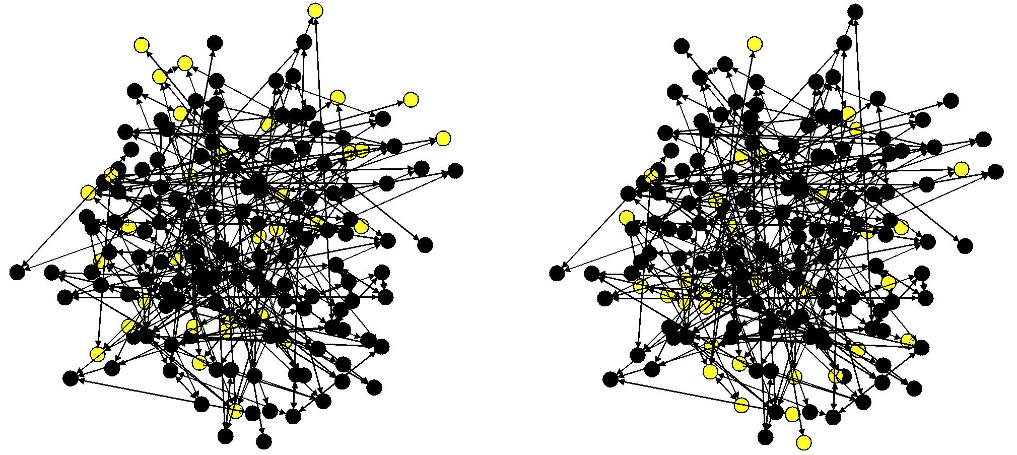
• An epidemic: At time $t=0$, an arbitrary subset of nodes is infected. The infection then spreads according to a standard suceptible-infectedmodel (Ganesh et al. (2005)). That is, infected nodes infect their neighbors according to an exponential clock set on each edge. We denote the set of infected nodes at time $T$ as $S=S(T)$, and the infection size as $|S|=\alpha(N)N$. At this time, each infected node reports it is infected with probability $q(N)$. We denote the set of truly reporting nodes by $S_{r}\subseteq S$, and thus call $S\setminus S_{r}$ the false negatives. In addition, there are $f|S_{r}|$ nodes, picked uniformly over the network, that also report infected. The intersection of these nodes with $S^{c}$, represent false positives. A reporting process illustration is presented in Fig 2.1.

• Uniform reporting: Each node, independently of all others, reports an infection with some probability. The problem is most interesting when this probability is chosen so that the expected numbers of reporting nodes in each scenario match.

Thus in summary, the key parameters that define our setting are as follows: $N$ is the total number of nodes; $\alpha(N)$ is the fraction of nodes ultimately infected, denoted by $S$; $q(N)$ is the probability that a node in $S$ will report, and hence $(1-q)$ is the false negative rate; $f$ controls the fraction of false positives, which scale as $f/(1+f)$, and hence goes to $100\%$ as $f\rightarrow\infty$.

Many settings exhibit the above structure. Influenza and allergies are known to produce similar symptoms – without a professional diagnosis, these may often be confused, even more so when the only indication of either is absence from work or school. Influenza of course is the epidemic, whereas allergies affect near and distant neighbors independently. Technology adoption shares similar traits. Word of mouth advertising spreads like an epidemic, where as mass media advertisement affects customers independently.

Figure 2.1: An illustration of the epidemic reporting process. The contagion spans the red nodes, numbered by the infection order, starting from “patient zero”, numbered by one. The infected network fraction is $\alpha=0.25$ . There are two truly reporting nodes, $\left(q=0.4\right)$ denoted by red and yellow stripes. In addition, there are two more false positives $\left(f=1\right)$, in black and yellow stripes.

A sample reporting map of the two processes is displayed in Fig. 2.2. When the reporting probability increases, $q(N)\rightarrow 1$, there exists a large connected component with a ball-like shape about the set of “patient-zero”s and the problem is easier. Likewise, the problem is more difficult when $f(N)\rightarrow\infty$, as the truly reporting nodes are washed out by the sea of falsely reporting nodes. We describe a class of algorithms that is shown to converge correctly even in settings where $q(N)\rightarrow 0$ and $f(N)\rightarrow\infty$.

Figure 2.2: Reporting map samples. The reporting nodes are in yellow. (left) A reporting sample in a uniform reporting setting. (right) An epidemic reporting scenario map. It is difficult to distinguish between the two hypotheses visually.

2.2 Prior Work

The predictive (forward) analysis of our SI model, as in (Ganesh et al. (2005)), is tightly related to results in First Passage Percolation theory (Blair-Stahn (2010)). These and related works focus on modeling the epidemic spread characteristics, for example, estimating the infection rate for different topologies (e.g., Gopalan et al. (2011)), predicting the first time the infection exceeds a given boundary, and so on. These are, therefore, prediction problems, or forward problems: given the initial conditions, predict what happens in the future.

Our work focuses on the inverse question: given (a noisy version of) what happened, solve the inference problem to decide if the process is an epidemic or a random illness. Recently, related inference questions have gained considerable attention. Of particular interest are estimating the model parameters, such as transmission rate, either by MCMC methods (Streftaris & Gibson ), or a Bayesian approach (Demiris & O’neill ). Another frequently discussed question is the identification of the epidemic source (e.g., Shah & Zaman ; Karamchandani & Franceschetti (2013)).

The work that most closely relates to ours paper is Milling et al. (2012, 2013). They consider a similar model, and seek to solve the same problem. The key differences here are that the algorithm and analysis are completely different, with some important consequences. In those works, the authors rely on tools from first passage percolation, which in some settings (for some graph topologies, for initial infection conditions) may be fragile. For example, it is not clear if the algorithms given there are able to handle large numbers of initial seeds. Our results in Section 5 indicate that our algorithm is largely insensitive to the number of initial infections, and works well for even hundreds of spread out “patients zero.” A second important difference comes on the algorithmic front. Our algorithm is inherently local. As we describe below, it essentially counts nodes with many infected neighbors, at a high level bearing similarity to triangle-counting as a proxy for graph clustering (Watts & Strogatz (1998)). This allows our algorithm to be run in parallel, and most significantly, requires only local knowledge of the graph – something that may be critical in applications. In Section 5 we compare the performance of our new algorithm, and find that both on synthetic (e.g., Erdos-Renyi) graphs as well as real-world networks (e.g., part of the Facebook graph) our algorithm produces statistically much better results, and significantly less computational cost. As we explain below, our algorithm’s running time scales with the number of reporting infected nodes, which may be far smaller than the number of total nodes.

2.3 Our Contributions

There are two factors which control the “difficulty” of the hypothesis testing problem we have posed. First, the more the false negatives (i.e., the smaller the set $S_{r}$), the more the epidemic statistically resembles the random illness. Second, in the limit when all infected nodes report, the presence (or absence) of a large connected component is easy to test, and sufficient to solve the decision problem. Finally, the topology of the graph itself plays an important role. The more connected the graph is, the more the two processes become statistically identical. In the limiting case where the contact network is the complete graph, the two processes are indistinguishable.

From the algorithmic standpoint, there is a further regime of interest: the very small infection setting. It is interesting to understand in this setting, how well an algorithm using only minimal graph information, can perform.

Our contributions are statistical and algorithmic, and address both regimes discussed above. Specifically, the key contributions of this work are as follows.

• Algorithm: We provide a simple distributed algorithm that runs in time linear in the number of reporting infected nodes, can be easily parallelized, and requires minimal knowledge of the graph: each infected node is required to know only information about its local neighborhood.

• Statistical Performance: We give sufficient conditions for our algorithm to correctly identify the infection cause (epidemic or random). In particular, we give conditions that guarantee that our algorithm succeeds even when the number of infected nodes is a $O(N)$, i.e., a constant fraction of all the nodes. We also consider the small-infection regime. We show here that our algorithm succeeds even if each node only knows the graph up to its 1-hop neighbors.

• Experiments: we provide experiments on synthetic (random) graphs, as well as real-world graphs. We show that our algorithm’s performance is at least as good as the theory predicts. Moreover, its efficiency allows it to scale easily to very large networks. We compare to state-of-the-art and demonstrate that our algorithm is both faster and more accurate.

3 The Algorithm: Hotspot Aggregator

The intuition behind our algorithm is simple: in an epidemic, having sick neighbors is more common than in the case of a random illness.

Definition 1.

For $B_{i}(l)$ denoting the radius-$l$ ball about node $i$, and $NN_{i}(K)$ denoting the set of the $K$ nearest neighbors of node $i$, we define the following indicator random variables:

$$H_{i}^{NN}(K,s)=\begin{cases}1&\left|\{v\in NN_{i}(K)\cap S\}\right|\geq s\\ 0&\text{otherwise}\end{cases}$$

and a similar indicator, $H_{i}^{B}(l,s),$ for the radius-$l$ ball. These indicators are true only if there are enough (more than $s$) reporting nodes in the immediate neighborhood of $i$. These are equivalent with appropriate correspondence of $l$ and $K$, and so we use them interchangeably. If the indicator evaluates to 1, we call node $i$ a hotspot. The above intuition suggests that there are more hotspots in an epidemic than in a random infection. Thus the number of hotspots, i.e., the sum of these indicators over reporting infected nodes, suggests a threshold test, that can correctly classify the infection cause. This is precisely the crux of Hotspot Aggregator Algorithm, Algorithm 1.

Input: Threshold values $K,\>T.$

Output: An epidemic or a random reporting scenario

  ${\rm counter}\leftarrow 0$

  for $i=1$ to $N_{\mbox{{\tiny{reporting}}}}$ do

     ${\rm counter}\leftarrow{\rm counter}+H^{NN}_{i}(K,K)$

  end for

  if ${\rm counter}>T$ then

     return epidemic

  else

     return uniform reporting

  end if

Algorithm 1 The hotspot aggregator

Theoretical/Practical Implementation. The algorithm depends on the nearest-neighbor threshold value $K$, and the parameter $T$. The theorems that make up our main results in the next section, demand a careful choice for $K$ and $T$ that requires approximate knowledge of the false positive rate and the graph topology. As we detail in the appendix, for some topologies the values for $K$ and $T$ can be computed analytically. More generally, the optimal values can be computed through simulation. On the other hand, our experimental results in Section 5 suggest that the algorithm’s performance is quite stable. For instance, choosing $K$ corresponding to the $r$-hop neighborhood in a graph, for $r=2,3$ yields uniformly good computational results (see Section 5 for more).

Algorithm Information and Complexity. The complete graph information (its global structure) requires $O\left(N^{2}\right)$ to encode. In contrast, our algorithm requires only the vector $C$, which contains the number of reporting nodes within each local environment. The length of $C$ is the number of reporting nodes, denoted by $N_{\mbox{{\tiny{reporting}}}}$, where for many cases of interest, $N_{\mbox{{\tiny{reporting}}}}$ can be as small as $O(\log(N))$ or even lower. In addition to being a parsimonious representation of the information required by our algorithm, the vector $C$ may be reconstructed by knowledge of only the local neighborhood of the reporting nodes, rather than the whole graph. As discussed above, such local information is often the only reasonably accessible/reliable information.

The algorithm’s complexity is $o(N_{\mbox{{\tiny{reporting}}}})$ and it scales with the number of reporting nodes (which, again, is typically vanishingly small compared to the to the number of nodes in the network). Similarly, the memory requirement is also very small and therefore this algorithm is easily scalable.

Algorithm Performance. As the noise increases, so does the difficulty of the decision problem . In the next section we discuss the convergence properties of the algorithm under extremely noisy conditions and present specific choices for the parameters $T$ and $K$. We show that under relaxed topological constraints, the algorithm converges correctly even when the number of falsely reporting nodes is $\Theta(N)$, irrespective of the number of truly reporting nodes, which may be even $\omega(1)$. In an extreme scenario, where the number of false positives is $\Theta(N)$ greater than the truly reporting nodes number, Corollary 4 shows the local environment about every reporting nodes should contain $\Theta(\log N)$ nodes. However, if the number of falsely reporting nodes is $o(N)$, then it possible to apply the algorithm on a local environment which contains only a finite number of nodes, as shown in Theorem 5.

4 Main Results: Correctness & Convergence

Before we proceed, we require some preliminary definitions.The infection boundary is the set of infected nodes that have a non-infected node in their local neighborhood. An alternative definition for a boundary is a set of infected nodes for which at least one of the $k$ nearest neighbors is not infected.

Definition 2.

The $l$th order boundary $\partial S(l)$ is a subset of infected nodes, $\partial S(l)\subseteq S$, such that for every $i\in\partial S(l)$ we have $B_{i}(l)\cap S^{c}\neq\emptyset$, i.e., there exists $j\notin S$ in the ball $B_{i}(l)$. Alternatively, the $k$th order border set is a subset of infected nodes, $DS(k)\subseteq S$, such that for every $i\in DS(k)$ we have $NN_{i}(k)\cap S^{c}\neq\emptyset$. We denote by $\gamma(k)=1-\left|DS(k)\right|/|S|$ the fraction of interior nodes, i.e., nodes for which their local neighborhood is contained in the infected region.

As discussed in the introduction, this decision problem’s difficulty increases with the number of false positives and false negatives. The most challenging setting is when the number of false positives is $\Theta(N)$, regardless of the number of truly reporting nodes, which may be $\omega(1).$ We call this the dense regime. As shown in our first theorem, in this regime, if $\gamma(K)$ is non zero for $K=O(\log N)$, the algorithm converges correctly. Alternatively, assume the number of truly reporting node is also $\Theta(N)$. If $\gamma\left(K\in O(1)\right)$ is non zero then the algorithm converges as well.

The algorithm succeeds when the number of hotspots in the epidemic and random scenarios differ significantly. The hotspot indicator is a Bernoulli random variable, hence computing the expectation of their sum across reporting nodes is straightforward. However, these Bernoulli random variables are correlated, in proportion to their graph distance to each other. Thus the key technical portion of the proof involves controlling the variance of this sum, by appropriately harnessing large deviation results for sums of correlated random variables.

Theorem 3.

Assume the number of reporting nodes, whether truly reporting or falsely reporting, is $\Theta(N)$. Assume there exist values $K,\gamma$ such that

a) $\Pr\left(\gamma(K)\neq 0\right)\rightarrow 1$ for $N\rightarrow\infty$

b) $K=\left\lceil\log(\gamma^{-1}\left(f+1\right))\right\rceil.$

Then, the hotspot aggregator algorithm with parameters $K$ and

$$T = \frac{N_{\mbox{{\tiny{reporting}}}}}{2}\left(\frac{\gamma p_{in}^{K}}{\left(f+1\right)}+p^{K}\right)$$

classifies correctly with high probability. The type I error and type II error decay rates are $o\left(\exp(-cN_{\mbox{{\tiny{reporting}}}})\right)$, where $c$ is a constant that depends on the problem parameters.

As an immediate corollary of this result, we see that in the large-infection-regime, our algorithm succeeds even as the numbers of false negatives and positives are overwhelmingly greater than the number of truly infected reporting nodes. The proof follows immediately from the theorem, and the details are deferred to the appendix.

Corollary 4.

For a large infection with $\Theta(N)$ infected nodes (i.e., $\alpha=\mbox{$\Theta$(1) }),$ the algorithm converges correctly if conditions (a) and (b) above are satisfied, even when the reporting probability goes to zero and noise ratio goes to infinity, i.e., $q\in\omega\left(N^{-1}\right)$ and $f\in\omega\left(q^{-1}\right)$.

In particular, if the number of truly reporting nodes is $\Theta(N)$, then the algorithm converges correctly if $\gamma(K=const)>0$. Alternatively, the algorithm converges correctly for every network such that $\gamma(K=2\log N)>0$. This holds, for example, for grids and tree like networks, even if the noise is $f\in\Theta(N)$.

Proof.

Denote the epidemic (uniform reporting) indicator as $\mathcal{I}$ (respectively, $\tilde{\mathcal{I}}$ ), the reporting probability of an infected node in the epidemic scenario by $p_{in}$.and the node reporting probability in the uniform reporting scenario as $p$. In the uniform reporting scenario, the probability that a local hotspot indicator is true is

$$\Pr\left(|\{v\in NN_{i}(k)\cap S_{\mbox{{\tiny{reporting}}}}\}|\geq k\right) = p^{k}.$$

Therefore, the expected number of hotspots in the uniform reporting case $\sum_{i\in V}H_{i}|\tilde{\mathcal{I}}$ is

$$\mathbb{E}\left(\sum_{i\in V}H_{i}|\tilde{\mathcal{I}}\right)=\sum_{i\in V}\mathbb{E}\left(H_{i}|\mathcal{\tilde{\mathcal{I}}}\right)=N_{\mbox{{\tiny{reporting}}}}p^{k}.$$

In the epidemic setting, the hotspot number is greater than the interior (non-boundary) hotspot number. Therefore,

$$\mathbb{E}\left(\sum_{i\in V}H_{i}|\mathcal{I}\right)\geq\mathbb{E}\left(\sum_{i\in S,i\notin DS}H_{i}|\mathcal{I}\right)\geq\frac{\gamma N_{\mbox{{\tiny{reporting}}}}}{\left(f+1\right)}p_{in}^{k}$$

where we used the fact that the expected number of truly reporting nodes is $N_{\mbox{{\tiny{reporting}}}}/\left(f+1\right)$ and applied Lemma 9 (stated in the appendix).

Set $T=N_{\mbox{{\tiny{reporting}}}}\left(\frac{\gamma p_{in}^{k}}{\left(f+1\right)}+p^{k}\right)/2$. Applying Lemma 6, choose

$$K\geq\log(\gamma^{-1}\left(f+1\right))\geq\log(\gamma^{-1}\left(f+1\right))p/p_{in}.$$ (4.1)

Now the key step is to evaluate the error rates, despite the correlation. To do this, we use a Hoeffding-like large deviation theorem (see Corollary 2.6 in Janson (2004)) for graph-structured correlation decay patterns. We can form a dependence graph $\Gamma$ among these $N_{\mbox{{\tiny{reporting}}}}$ random variables, drawing an edge between any two non-independent random variables. Note, then, that for each two nodes, $i$ and $j$, the hotspot indicators $H_{i}$ and $H_{j}$ are independent iff the corresponding environments $B_{i}$ and $B_{j}$, or $NN_{i}$ and $NN_{j}$ are disjoint. The number of nodes in each local environment of the $k$ nearest neighbors of $i$ is also $k$, so the number of nodes with disjoint local environments is at least $N-k^{2}$. In other words, the maximal node degree in $\Gamma$ is $k^{2}$.

Set $P=p^{K},P_{in}=\gamma p_{in}^{k}/(f+1)$. Then, adapting some concentration inequalities from Janson (2004), we can show that the type I error, $E_{I}:=\Pr\left(\sum_{i\in V}H_{i}|\tilde{\mathcal{I}}\geq T\right)$ is bounded by

$$E_{I}\leq\exp\left(-N_{\mbox{{\tiny{reporting}}}}\frac{\left(P_{in}-P\right)^{2}}{16\left(K^{2}+1\right)\left(P+\left(P_{in}-P\right)/6\right)}\right)$$

In the epidemic scenario, the total number of hotspots is at least as great as the number of interior hotspots. Therefore, the type II error is bounded by

$$E_{II}=\Pr\left(\sum_{i\in V}H_{i}|\mathcal{I}<T\right)\leq\Pr\left(\sum_{i\in S,i\notin DS}H_{i}|\mathcal{I}<T\right)$$

and similarly, the latter quantity is bounded by

$$\exp\left(-N_{\mbox{{\tiny{reporting}}}}\frac{\left(P_{in}-P\right)^{2}}{16\left(K^{2}+1\right)P_{in}}\right)$$

As shown in the appendix, these errors tend to zero under the conditions of this theorem. ∎

Applying Theorem 3 and Corollary4. As with the algorithm, applying the theorem or corollary requires calculating values of $\gamma(K)$ and $K$. As we show in the appendix, $\gamma(K)$ can often be explicitly (analytically) computed, and if that is not available, it can be easily computed numerically. In the appendix, we also present explicit instructions on the application of the hotspot algorithm for general networks, including specific finite size networks for which the statistical ensemble is unknown. When $\gamma(K)$ is known, one can simply find the minimal value of $K$ such

$$K\geq\log\left(\gamma(K)\right)+\log\left(f+1\right),$$

and substitute the corresponding value in the threshold. For example, for $d$-dimensional grids one can choose $K=\left\lceil\log(f+1)\right\rceil$ and

$$T=\frac{N_{\mbox{{\tiny{reporting}}}}}{2}\left(\frac{p_{in}^{K}}{\left(f+1\right)}+p^{K}\right),$$

while for a tree like network, such as an Erdos-Renyi network, choose $K$ such that $K\geq\log K+\left\lceil\log(f+1)\right\rceil$ and

$$T=\frac{N_{\mbox{{\tiny{reporting}}}}}{2}\left(\frac{p_{in}^{K}}{K\left(f+1\right)}+p^{K}\right).$$

If the function $\gamma(K)$ is not known or if it difficult to describe analytically and solve for $K,$ one can apply the bound $\gamma(K)\geq 1/\alpha N$ in eq. 4.1 and obtain a corresponding value for the threshold $T$.

As long as the probability to find a node for which the local environment is contained in the infected region is non-zero, the algorithm converges correctly. This is a very lenient requirement, which only fails for nearly full-mesh graphs, such that with high probability, for every ball, either there are less than $\log N$ nodes, $|B_{i}(l)|\leq\log N$, or the number of nodes in the ball is infinitely higher than $\log N$, $\log N/|B_{i}(l)|\rightarrow 0$ . Indeed, an alternative description for uniform reporting is a contagion on an underlining full mesh grid, and in this case the two processes are identical.

Small Infections

We now consider the setting of very small infections, and prove that in these settings, one can take $K$ to be a constant ($K\in\Theta(1)$), and moreover can choose this constant so that even the presence of a single hotspot indicates an epidemic infection.

Theorem 5.

Assume the total number of reporting nodes, is $N^{1-\beta}$, while the number of truthfully reporting nodes is $N^{\rho}$ and the truly reporting probability is $q(N)=N^{-\mu}$. Set $K=\left\lceil 1/\beta\right\rceil-1$ . If $\gamma(K)\in\omega\left(\log^{-1}(N)\right),$ then the hotspot aggregator algorithm with parameters $K$ and threshold $T=1$ classifies correctly with high probability if $K\mu\leq\rho.$ In particular, if $1>\beta>0.5$, than the hotspot algorithm with $K=1$ classifies correctly under the same conditions.

In this last case, the algorithm simply counts the expected number of infected neighboring pairs.

Proof.

For each two nodes, $i$ and $j$, the hotspot indicators $H_{i}$ and $H_{j}$ are independent iff the corresponding environment $B_{i}$ and $B_{j}$ are disjoint, $B_{i}\cap B_{j}=\emptyset$, otherwise they are positively correlated. In the uniform reporting scenario, define the probability that all the hotspot indicators are false as $P_{ep}\triangleq\Pr\left(\forall i\in N_{\mbox{{\tiny{reporting}}}},H_{i}=0\right)$. The probability for such event is bounded by:

$$P_{ep} \geq \prod_{i=0}^{N_{\mbox{{\tiny{reporting}}}}-1}\Pr(H_{i}=0,H_{j}=0|B_{i}\cap B_{j}=\emptyset)$$

$$= \left(1-p^{k}\right)^{N_{\mbox{{\tiny{reporting}}}}}.$$

Therefore, as $p\rightarrow 0$ ,$N_{\mbox{{\tiny{reporting}}}}\rightarrow\infty$

$$\Pr\left(\forall i\in N_{\mbox{{\tiny{reporting}}}},H_{i}=0\right)\rightarrow\exp\left(-p^{k}N_{\mbox{{\tiny{reporting}}}}\right)$$

According to the central limit theorem, $N_{\mbox{{\tiny{reporting}}}}=pN$ with high probability. By Applying Lemma 9 and choosing $k$ such that $p^{k}\in O(N^{-1})$, we have $\Pr\left(\forall i\in N_{\mbox{{\tiny{reporting}}}},H_{i}=0|\mathcal{\tilde{\mathcal{I}}}\right)\rightarrow 1.$

Similarly to Theorem 3, set $P_{in}=p_{in}^{k}$, $N^{\prime}_{\mbox{{\tiny{reporting}}}}=\gamma N{}_{\mbox{{\tiny{reporting}}}}/(f+1)$. In the epidemic setting, we can again apply Corollary 2.6 in Janson (2004), but now with a deviation of $t=N^{\prime}_{\mbox{{\tiny{reporting}}}}P$.

Then, the type II error is bounded by

$$E_{II}\leq\exp\left(-\frac{N^{\prime}_{\mbox{{\tiny{reporting}}}}P\left(1-\left(K^{2}+1\right)/4N\right)}{2\left(K^{2}+1\right)}\right).$$

The type II error tends to zero if $N^{\prime}_{\mbox{{\tiny{reporting}}}}P\rightarrow\infty.$ The latter condition can also be written as $q\alpha\gamma\left(q^{K}+\left(\alpha qf\right)^{K}\right)\in\omega\left(N^{-1}\right)$, while the condition for the type II correct convergence is $\left(\alpha qf\right)^{K+1}\in O(N^{-1}).$ ∎

In particular, if $N_{\mbox{{\tiny{reporting}}}}/N\in O(N^{-0.5})$, and $q^{2}\alpha\in\omega\left(N^{-1}\right)$ then it is sufficient to choose $K=1$, i.e., to count the number of infected nearest neighbors pairs.

This result is particularly useful for small infections (for example, $\alpha\in\Theta\left(N^{-0.3}\right)$). It shows that it is possible to detect epidemics using the hotspot aggregator algorithm even when the ratio of the number of false positives to the number of infected nodes tends to infinity (for example, $f\in\Theta\left(N^{0.7}\right)$), and the ratio of truly reporting nodes number to the number of infected nodes tends to infinity (for example, $q\in\Theta\left(N^{-0.3}\right)$), a quadratic “needle in a haystack” scenario.

Finally, note that the requirement for the algorithm convergence is that the boundary would not contain all the nodes. Therefore, even if multiple sources of an epidemic exist, then as long as this condition is satisfied, the algorithm converges correctly. Put differently, the hotspots aggregator will converge correctly as long as there are sources that had the chance to infect their local environment, rather than infect a large portion of the network. Hence, this algorithm is able to identify and nip contagions in the bud.

Next, we deploy this algorithm on both random network models, such as Erdos-Renyi networks or scale-free networks, and real-world networks, such as an enterprise email network, the Internet AS topology and Facebook.

5 Experiments

We perform empirical tests of our algorithm on both synthetic and real data. We focus on demonstrating its accuracy, running time and scalability in numerous settings. These simulations also demonstrate the ease-of-use of our algorithm in real experiments. While the theorems themselves require some care in choosing the parameters of the algorithm, here we find that 1, 2, and 3-hop local neighborhoods perform extremely well across a wide range of settings, including the setting of an overwhelming number of false positives, and the setting of up to 200 infection seeds (initial infected nodes).

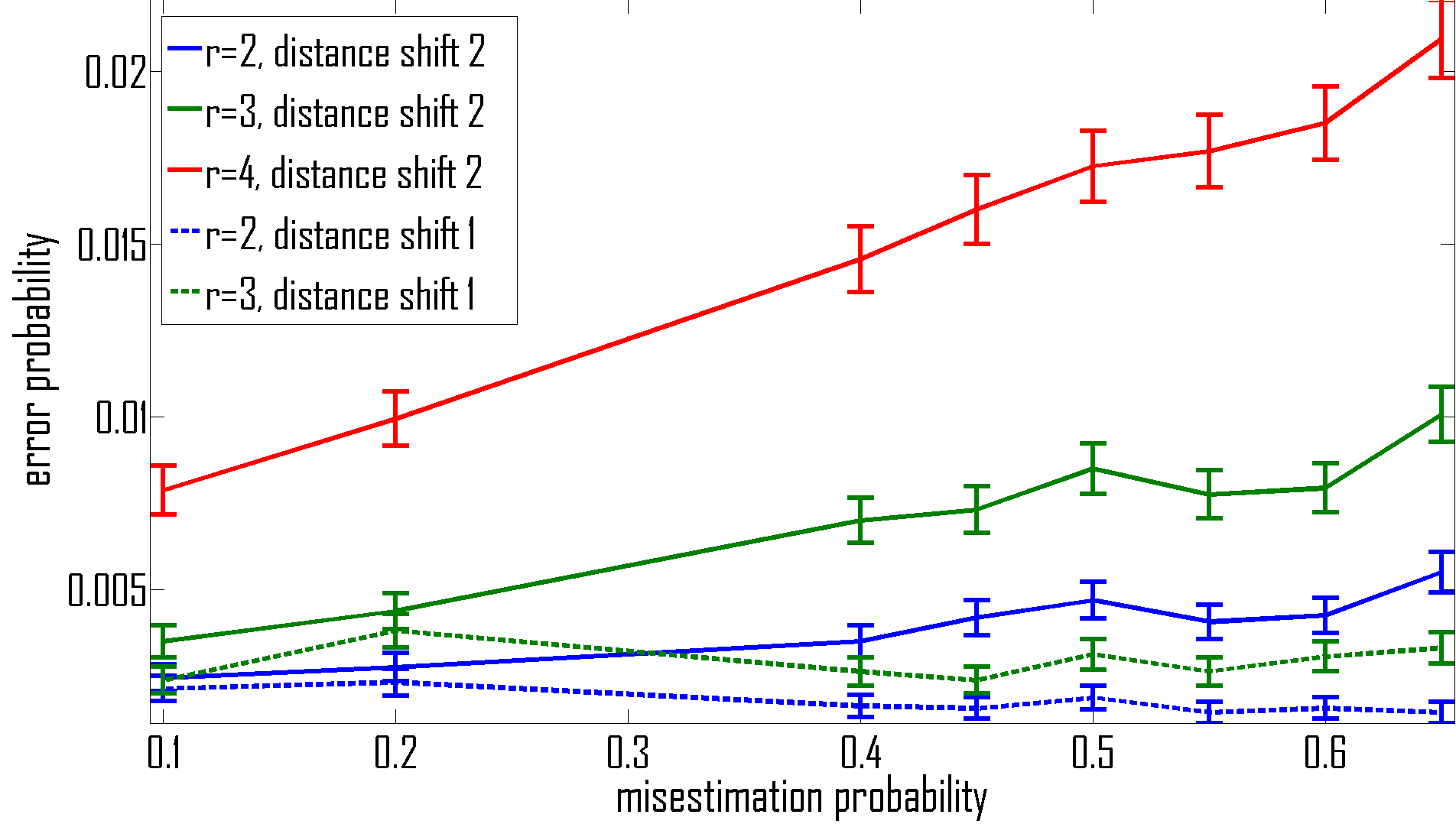
Synthetic Graphs. We consider the algorithm performance in the acute regime, where the number of false positives and false negatives each tends to infinity. We tested this (Fig. 5.1) on an Erdos-Renyi graph in the regime where the giant component emerges, $G(N=8000,p=2/N$) (Durrett (2010)). The error rate decays rapidly as the size of the graph increases, as predicted by Theorem 5, even as the fraction of truly reporting nodes among the reporting nodes tends to zero. Moreover there are infinitely more false negatives than true positives, as the network size increases. We also compare against the Median-ball-algorithm given in Milling et al. (2013). While the Median algorithm may be converging, we see that the convergence of our algorithms for $l=1,2,3,4$ is remarkably faster.

Interestingly, in this experiment, the $l=4$ version of our algorithms seems to have a slightly worse performance compared to $l=1,2$. This is likely because the regime of $G(N,p)$ we consider has diameter $\Theta\left(\log N\right)$, and thus even 4-hop neighborhoods are considerable in size.

In real-world networks, the degree distribution often follows a power law. For random power law networks, the network diameter is, like in the $G(N,p)$ , $\Theta(\log N)$, or even $\Theta(\log\left(\log N\right))$ (Cohen & Havlin (2003)). In such small-world networks, choosing a large ball radius deteriorates inference performance due to an overflow of the local ball about an infected node to an uncontaminated region.

Figure 5.1: The mean error rate for different ball radii for an Erdos Renyi graph $G(N,p=2/N)$. In this configuration, the number of false reporting nodes tends to infinity, while the fraction of truly reporting nodes among the reporting nodes tends to zero. In addition, the true reporting probability tends to zero, so that the number of false negative is infinitely higher than the number of true positives. Furthermore, the epidemic size is small, $O(N^{0.3})$. The simulation details are elaborated in the appendix.

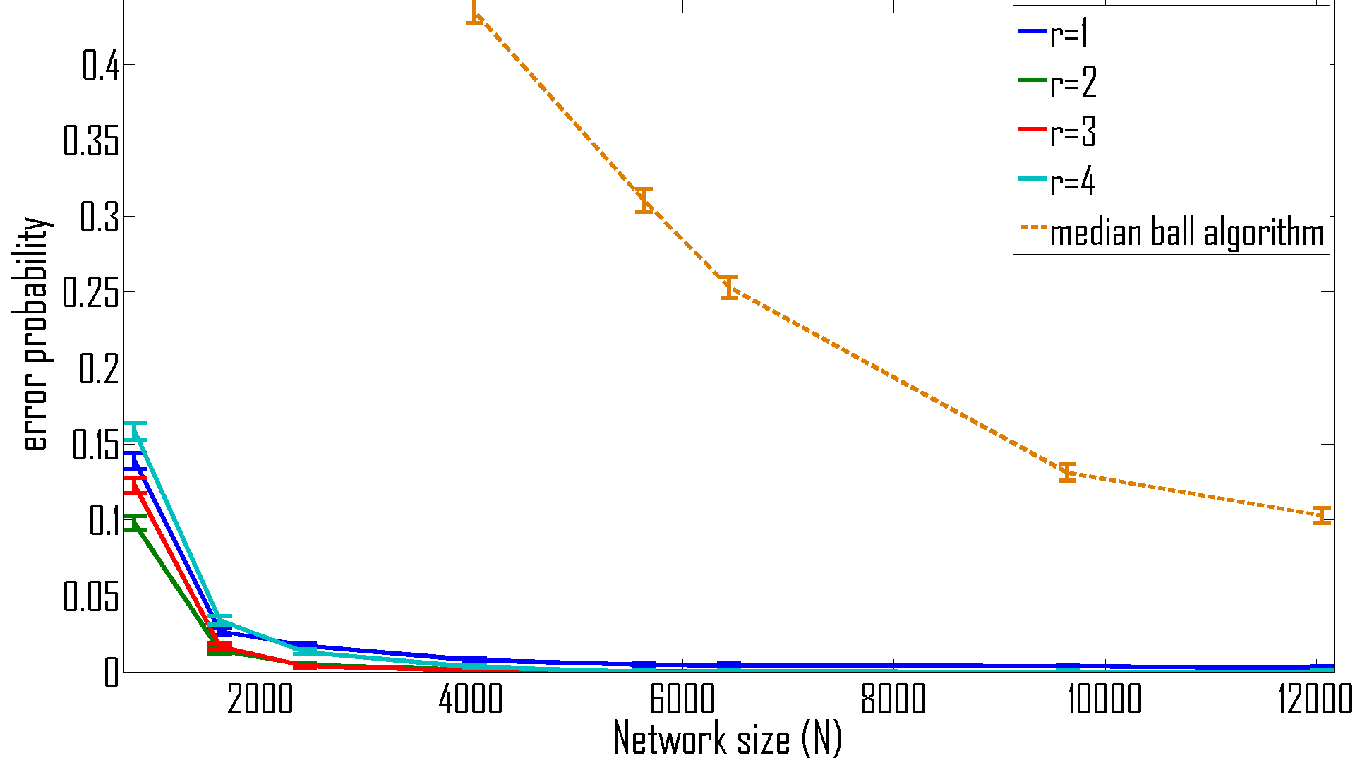
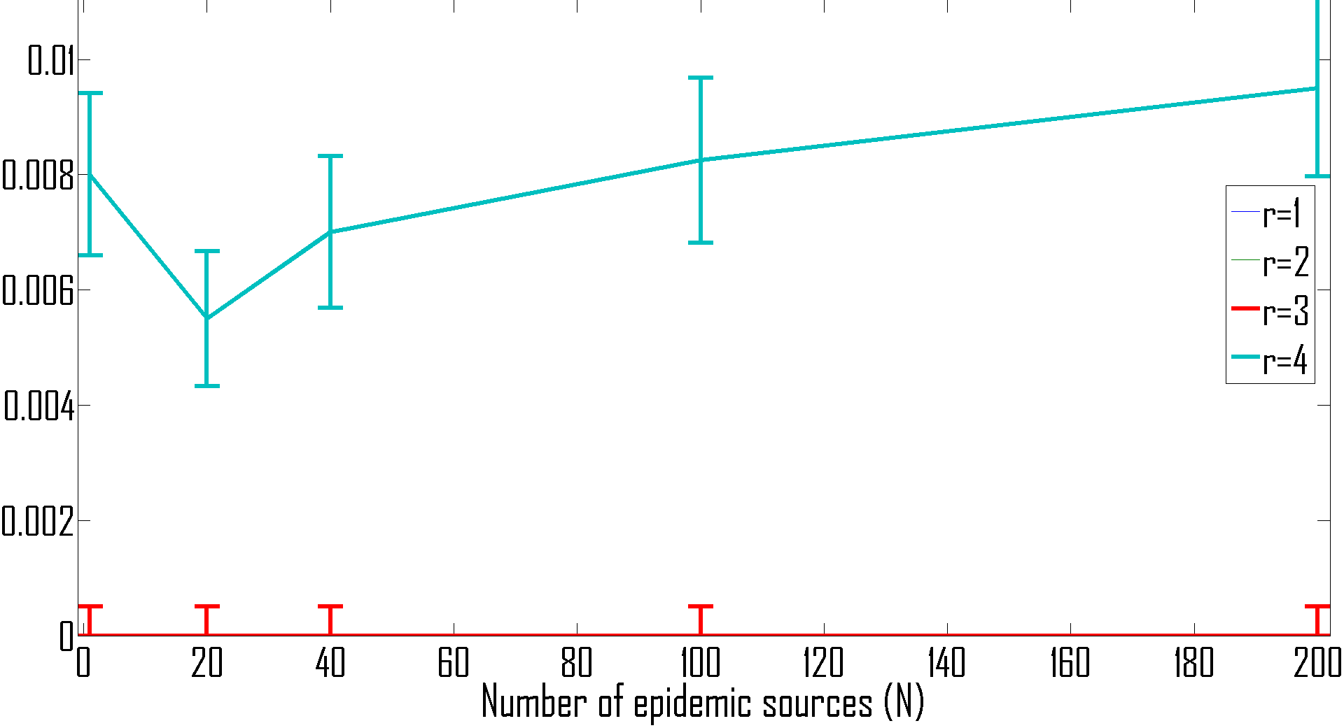
Real World Graphs. We next consider a real world graph, namely, the enterprise email network of Enron employees (Klimt & Yang ). In part, this is motivated by the fact that many computer viruses spread by email attachments. Figure 5.2 shows the setting of a small infection, with a very large fraction of false negatives, a large majority of false positives, and many initial sources of infection. Our results demonstrate the stability of our algorithm with respect to the number of initial infection seeds. Even with as many as 200 initial seeds, the performance of our algorithm is hardly affected. We note again a better performance for radius values $r=1,2,3$ in our algorithm; this is for the same reason as discussed above.

Additional instances of diffusive processes are the sharing of viral media and the adoption of memes on social networks. We examined the identification of such phenomena by testing our algorithm on a network of $63K$ Facebook contacts (Viswanath et al. (2009)). Finally, cascades of router failures due to misconfiguration or BGP attacks is a major security concern. We have performed experiments on these graphs as well, but for space concerns defer these to the appendix.

Figure 5.2: The mean error rate as a function of the number of epidemic sources for Enron email network. The network is comprised of $N=33,696$ nodes. The number of infected nodes is small, $0.06N$, and the number of truly reporting nodes is miniscule, $0.003N$. Finally, for each truly reporting node there are $8$ false positives ($f=8$). Even in this challenging situation, the error rate is low.

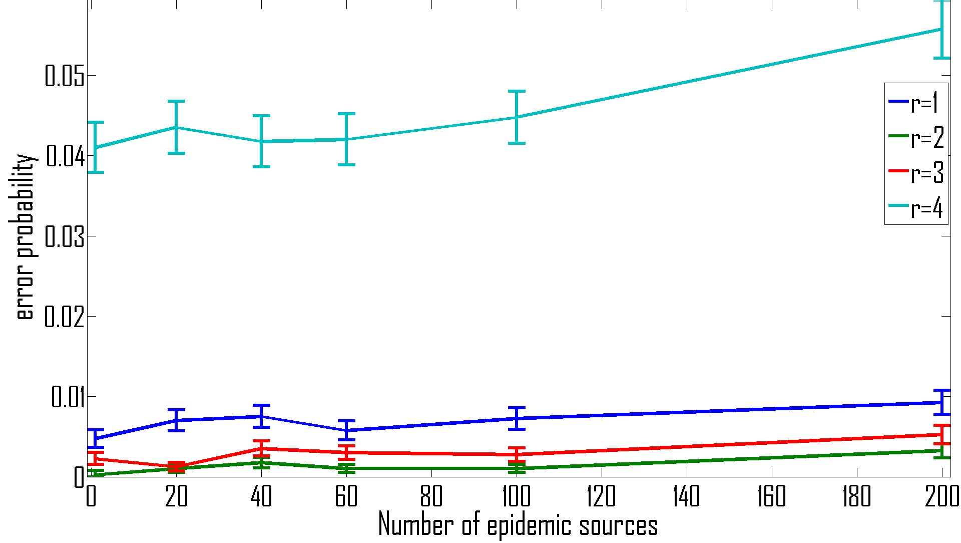
Last, we tested our algorithm in the presence of noisy network information, to test robustness to knowledge of local neighborhoods. Indeed, a person may erroneously estimate the distance to her peers, consequently resulting in an incorrect set of nearest neighbors, or the deformation of the ball centered about her. In our experiments, we account for the effect of noisy network information by allowing an expected fraction of the conceived inter-node distances to increase or decrease by $d$ (when the unmodified distance is greater than $d$). Consequently, the inference algorithm is performed on a different network than the one the epidemic evolved on. Note that such a modification is not symmetric, as one node may correctly estimate the distance to its peer, while its peer may not. The error rate of our inference algorithm is present in Fig. 5.3. The results here show that our algorithm is robust to such noisy network knowledge.

In an epidemic scenario, if a reporting node is deep in the infected region, there exists some buffer to the uninfected nodes at the contagion border, and the overestimation effect should be negligible. In contrast, if the reporting node’s exterior shell is close to the border, then the reporting node may mistake an uninfected node as a member of its local ball and performance may deteriorate. Therefore, we expect that the type II error should increase with the ball radius and the misestimation rate, expressed in either increased misestimation probability or the true distance deviation. These two effects are observed in Fig. 5.3. Finally, the type I error is unaffected by this type of topological noise.

Figure 5.3: The error probability under additional topological noise for an Erdos Renyi network $G(N=4000,p=2/N)$. The mean error is plotted against the probability that a node will estimate its distance to another node. The fault is equally likely to be an overestimate or underestimate of one (dashed lines) or two (solid lines) from the true nodes distance. The number of infected nodes is about $0.2$ of the whole population of $N=4000$. The number of true positives is $0.06N$, while the number of false positives is $0.08N$.

6 Conclusions

Our world becomes increasingly interconnected by multiple different networks. While this interconnection speeds information transfer and facilitates communication, is it also increases the likelihood of contagion outbreaks. Depending on the context, such outbreaks may be computer viruses, opinion trends, or epidemics such as malaria. The hair-trigger identification of these diffusive processes is crucial and one may be forced to rely on a single reporting map snapshot in time. Furthermore, a complete knowledge of the underlying network graph is generally unrealistic. We have provided both analytical proofs and experiments on real data, showing that the hotspot aggregator algorithm solve this statistical inference problem in its dire setting on a wide variety of network and settings. We have shown that this algorithm classifies correctly even when the rate of false positives and false negatives is infinitely higher than the number of true positives, as well as in the presence of multiple sources of epidemics.

We have simulated this algorithm both on random networks, such as Erdos-Renyi graphs or scale-free graphs, and on real world networks, such as Facebook, the Internet AS-topology and Enron email chain. Our simulations exhibit the exponential decrease of the error rate with the size of the network, as predicted. In practice, the error rates are extremely low, even when there are errors in estimating the network structure. Finally, the complexity of our algorithm is low, and it is clearly scalable, as shown by the low error rate on the Facebook network of over $60K$ nodes.

Appendix A Appendix A - Additional lemmas

Lemma 6.

Denote the reporting probability of an infected node in the epidemic scenario by $p_{in}$. Similarly, denote the node reporting probability in the uniform reporting scenario as $p$. Then, $p_{in}>p.$

Proof.

First, note that

$$p_{in} = q+(1-q)\frac{fq\alpha}{1-q\alpha}$$

$$= q\left(1+(1-q)\frac{f\alpha}{1-q\alpha}\right)$$

while

$$p=\left(f+1\right)q\alpha$$

Therefore,

$$p_{in}-p > q+(1-q)\frac{fq\alpha}{1-q\alpha}-\left(f+1\right)q\alpha$$

$$= \frac{q}{1-q\alpha}\left(1-q\alpha+(1-q)f\alpha-\left(f+1\right)\alpha\left(1-q\alpha\right)\right)$$

$$= \frac{q}{1-q\alpha}\left(1-q\alpha-qf\alpha+f\alpha-f\alpha-\alpha+q\alpha^{2}+fq\alpha^{2}\right)$$

$$= \frac{q}{1-q\alpha}\left(\left(1-\alpha\right)(1+q\alpha+qf\alpha\right)$$

$$> 0$$

as $\alpha>0$.∎

Lemma 7.

The errors expressed in Theorem 3 tends to zero under the corresponding conditions.

Proof.

Set $P=p^{K},P_{in}=\gamma p_{in}^{k}/(f+1)$. According to Corollary 2.6 in Janson (2004) the type I error rate can be bounded by

$$E_{I}\leq\exp\left(-N_{\mbox{{\tiny{reporting}}}}\frac{\left(P-P_{in}\right)^{2}\left(1-\frac{\left(\Delta(\Gamma)+1\right)}{4N_{\mbox{{\tiny{reporting}}}}}\right)}{8\left(\Delta(\Gamma)+1\right)\left(1-P\right)\left(P+\left(P_{in}-P\right)/6\right)}\right)$$

where $\Delta(\Gamma)$ is the maximal degree of the dependency graph $\Gamma.$ However, $\Delta(\Gamma)\leq\max\{N_{\mbox{{\tiny{reporting}}}},K^{2}\}$ and therefore,

$$E_{I}\leq\exp\left(-N_{\mbox{{\tiny{reporting}}}}\frac{\left(P_{in}-P\right)^{2}}{16\left(K^{2}+1\right)\left(P+\left(P_{in}-P\right)/6\right)}\right)$$ (A.1)

Set $\delta=p_{in}-p.$ First, note that if $\lim\left(P-P_{in}\right)\neq 0$, then this expression tends to zero. Therefore, if $\lim\delta\neq 0$ for $N\rightarrow\infty$ than the type I error rate tends to zero.

Recall that

$$p_{in} \in \Omega\left(q+fq\alpha\right)$$

$$\delta \in \Theta(q)$$

$$p \in \Theta\left(fq\alpha\right)$$

And therefore in this case $q\in\Omega(1)$. Otherwise, assume that $\lim\delta=0$. If

$$\delta/p\rightarrow 0$$

or equivalently, $f\alpha\in\omega(1)$, the highly noise regime, then to first order in $\delta/p$

$$\left(P_{in}-P\right)^{2}\rightarrow p^{2k}\left(1-\frac{1}{\gamma(f+1)}\right)^{2}$$

with $\delta=p_{in}-p.$ Likewise, if $\delta/p\rightarrow const$, than we can write

$$p = g(N)\tilde{p}$$

$$\delta = g(N)\tilde{\delta}$$

where $\tilde{p}\rightarrow const\neq 0$ and $\tilde{\delta}\rightarrow const\neq 0$ and

$$\left(P-P_{in}\right)^{2}=g^{2K}(N)\left(\frac{\left(\tilde{p}+\tilde{\delta}\right)^{K}}{\gamma(f+1)}-\tilde{p}^{K}\right)^{2}$$

Therefore, for either $K=1$ or $K=2$ we have

$$\lim\left(\frac{\left(\tilde{p}+\tilde{\delta}\right)^{K}}{\gamma(f+1)}-\tilde{p}^{K}\right)^{2}\neq 0$$

and therefore $\left(P-P_{in}\right)^{2}\in\Theta(p^{2k})=\Theta(\delta^{2k})$.

Recall that with high probability $N_{\mbox{{\tiny{reporting}}}}=Np$. As,

$$E_{I}\leq\exp\left(-N\Theta\left(p^{2k+1}\right)\right)$$

if

$$\left(fq\alpha\right)^{2K+1}\in\omega(N^{-1}),$$

the type I error tend to 0 for $N\rightarrow\infty$. In other words, if $K$ is such that

$$\left(N_{\mbox{{\tiny{reporting}}}}/N\right)^{2K+1}\in\omega(N^{-1})$$

the error tend to 0. Alternatively, if $p/\delta\rightarrow 0$ then

$$\left(P_{in}-P\right)^{2}\rightarrow\left(\frac{\gamma\delta^{k}}{(f+1)}\right)^{2}$$

and therefore, if

$$\gamma^{2}q^{K}/f\in\omega(N^{-0.5})$$

then the algorithm converges correctly.

A similar calculation shows that if this condition holds, then the type II error tends to 0 for $N\rightarrow\infty$. Explicitly:

$$E_{II}\leq\exp\left(-N_{\mbox{{\tiny{reporting}}}}\frac{\left(P-P_{in}\right)^{2}\left(1-\frac{\left(\Delta(\Gamma)+1\right)}{4N_{\mbox{{\tiny{reporting}}}}}\right)}{8\left(\Delta(\Gamma)+1\right)P}\right)$$

and following similar reasoning

$$E_{I}\leq\exp\left(-N_{\mbox{{\tiny{reporting}}}}\frac{\left(P_{in}-P\right)^{2}}{16\left(K^{2}+1\right)P_{in}}\right)$$

and this expression has the same scaling properties as eq. A.1.∎

Corollary 8.

Consider a large infection, where the number of infected nodes is a constant fraction of the number of nodes, $\alpha=\mbox{$\Theta$(1) .}$ The algorithm converge correctly even when the reporting probability tends to zero as $q\in\omega\left(N^{-1}\right)$ while the noise ratio tend to infinity $f\in\omega\left(q^{-1}\right)$, as long as conditions a) and b) of theorem 3 are satisified.

In particular, if the number of truly reporting nodes is $\Theta(N)$, then the algorithm converges correctly if $\gamma(K=const)>0$. Alternatively, the algorithm converges correctly for every network such that $\gamma(K=2\log N)>0$, for example, grids and tree like networks, even if the noise is $f\in\Theta(N)$.

Proof.

Note that $f<N$. If $\gamma\neq 0,$ then $\gamma<1/\alpha N$. In particular, if the number of truly reporting nodes is $\Theta(N)$, then $f\in\Theta(1)$.Therefore

$$K\geq-\log(\gamma)+\log(f)$$

and substituting the corresponding values in Theorem 3 concludes the proof..∎

Lemma 9.

Consider a binomial random variable $X$ with expectation value $pN$ for $N\rightarrow\infty$. Then any sum of Bernoulli random variables $Y_{i}$ obeys

$$\mathbb{E}\left(\sum_{1}^{X}Y_{i}\geq c\right) \rightarrow \mathbb{E}\left(\sum_{1}^{M}Y_{i}\geq c\right)$$

$$\mathbb{E}\left(\sum_{1}^{X}Y_{i}\leq c\right) \rightarrow \mathbb{E}\left(\sum_{1}^{M}Y_{i}\leq c\right)$$

In other words, we can asymptotically replace the summation over random number of RVs in the summation over the mean number or RVs.

Proof.

Set $M=Np-\left(Np\right)^{2/3}$. First, note that

$$\mathbb{E}\left(\sum_{1}^{X}Y\geq c\right) = \mathbb{E}\left(\sum_{1}^{X}Y\geq c|X>M\right)\Pr(X>M)+\mathbb{E}\left(\sum_{1}^{X}Y\geq c|X\leq M\right)\Pr(X\leq M)$$

$$\leq \mathbb{E}\left(\sum_{1}^{X}Y\geq c|X>M\right)\Pr(X>M)$$

$$\leq \mathbb{E}\left(\sum_{1}^{X}Y\geq c|X=M\right)\Pr(X>M).$$

According to Hoeffding’s inequality

$$\Pr(X\leq M) \leq \exp\left(-\left(Np\right)^{1/3}\right).$$

and therefore

$$\mathbb{E}\left(\sum_{1}^{X}Y\geq c\right)\leq\mathbb{E}\left(\sum_{1}^{M}Y\geq c\right)\left(1-\exp\left(-\left(Np\right)^{1/3}\right)\right)$$

Similarly, we can apply Hoeffding’s inequality for $M=Np-\left(Np\right)^{2/3}$ in

$$\mathbb{E}\left(\sum_{1}^{X}Y\leq c\right) = \mathbb{E}\left(\sum_{1}^{X}Y\leq c|X>M^{\prime}\right)\Pr(X>M)+\mathbb{E}\left(\sum_{1}^{M}Y\leq c|X\leq M^{\prime}\right)\Pr(X\leq M)$$

$$\leq \mathbb{E}\left(\sum_{1}^{X}Y\geq c|X\leq M^{\prime}\right)\Pr(X<M)$$

while

$$\Pr(X\geq M^{\prime})\leq\exp\left(-\left(Np\right)^{1/3}\right)$$

and obtain

$$\mathbb{E}\left(\sum_{1}^{X}Y\leq c\right)\leq\mathbb{E}\left(\sum_{1}^{M^{\prime}}Y\geq c\right)\left(1-\exp\left(-\left(Np\right)^{1/3}\right)\right)$$

but both $M,M^{\prime}\rightarrow Np$ and this concludes the proof. ∎

Appendix B Appendix B - Algorithm application

In order to apply the algorithm, the parameters $K$ and $T$ must be specified, and the number of nodes in the local environment must be set. We assume that a good estimate for the reporting probability of an infected node, $p_{in}$, is known. Note that for large networks the reporting probability $p$ can be easily estimated according to $p=N_{\mbox{{\tiny{reporting}}}}/N$. Recall that $\gamma(K)$ is the fraction of infected nodes for which their $K$ nearest neighbor nodes are also infected is known.

We distinguish between two classes of networks. First we discuss large networks for which the function $\gamma(K)$ is known, whether numerically or analytically. As an example, consider an infinite constant degree tree with degree $d$. Assume that the infection, starting from the root, has infected all the nodes up to the $m$-th level. In this case, for every node that is deeper than the $m-l$ level of the tree, all the nearest $d^{l}$ are not infected. The fraction of such nodes is

$$\gamma(K=d^{l})\leq\frac{d^{m-l}-1}{d^{m}}\rightarrow d^{-l}$$

Therefore, $\gamma(K)=K^{-1}$.

As another example, consider a $d$ dimensional grid. In this case, the contagion is with high probability contained within an $l_{1}$ ball of radius $r=c|S|^{1/d}$, with $c\rightarrow const$ for $N\rightarrow\infty$ (Milling et al. (2012)). The number of nodes on the non-infected bordering nodes near the surface of such ball is $\Theta(r^{d-1})$. In addition a ball of radius $l$ contains $\Theta(l^{d})$ nodes. Therefore, the number of interior nodes is at least $\Theta(r^{d-1}l^{d})$. Hence,

$$\gamma\left(K\in\Theta(l^{d})\right)\leq\Theta\left(r^{-1}l^{d}\right)$$

Hence for balls of radii $K\in o\left(|S|^{1/d}\right)=o\left(\left(\alpha N\right){}^{1/d}\right)$ we have

$$\gamma(K)\rightarrow 1$$

In these cases, Theorem 3 provides a prescription for $K$ and $T$ when the number of reporting nodes is large, $\Theta(N)$, while if the number of reporting nodes is small, $o(N)$, the prescription in Theorem 5 applies

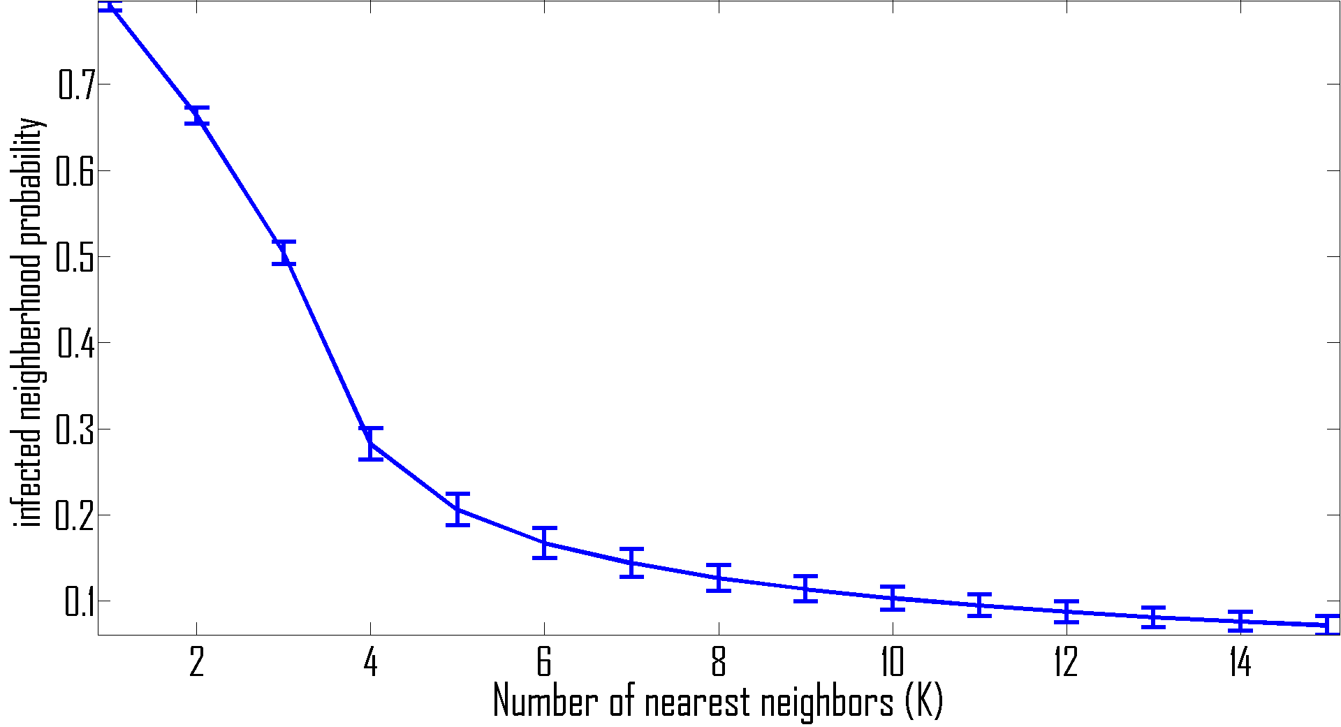
For a finite size network, that is not necessarily sampled from a statistical ensemble, $\gamma(K)$ might be not known apriori. Nevertheless,$\gamma(K)$ may be calculated at a preprocessing stage. This can be done by simulating epidemics according to the scenario details. Then, for each infected node, calculate the probability that $K$ of its neighboring nodes are infected, and average over all infected nodes. As an example, the $\gamma(K)$ function for the Internet inter-AS topology, which is often considered a scale free network, is presented in Fig. B.1. Note that for any network, and any value of $K,$ if there is an infected node that $K$ of its nearest neighbors are infected, then $\gamma(K)\neq 0$. In this case, $\gamma\geq 1/|S|$, where$|S|$ is the infection size. The maximal relevant value of $K$ is $\log(|S|)$, according to Theorem 3.

After this preprocessing stage, if the number of reporting nodes is large one applies Theorem 3 , or Theorem 5 otherwise.

Figure B.1: The probability $\gamma(K)$ that $K$ nearest neighbors of an infected node will be infected as well. The plot was generated for the Internet inter-AS graph, composed of $N\approx 27K$ nodes. Even for a small infection size $(|S|=0.06N$) the fraction $\gamma(K)$ is significant even up to the maximal relevant value of $K=\log(|S|)\approx 7.5.$

Finally, it is important to note that one can perform multiple tests with various values of $K$. If no epidemic occurred, then in all those tests the number of hotspots should be close to the expected number of a uniform reporting event. If any tests results is far from this value, then an epidemic occurred. This approach is particularly relevant if the critical requirement is high specificity, and if no information on the possible epidemic is available. Note that as there are at most $\log(N)$ tests, applying multiple tests does increase the algorithm complexity appreciably.

Appendix C Appendix C - Additional experiments

Figure C.1: The mean number of hotspots (and the standard deviation) as a function of $K$. The plot was generated for an Erdos Renyi graph $G(N=8000,p=2/N)$ and ball radius $l=3$. The simulation parameters are $\alpha=0.13,\>q=0.22$ and $f=1$. The plot was generated by Monte Carlo simulations of $2000$ trials for each scenario.

In this section we present additional simulations, some of which are described in the main body of this paper.

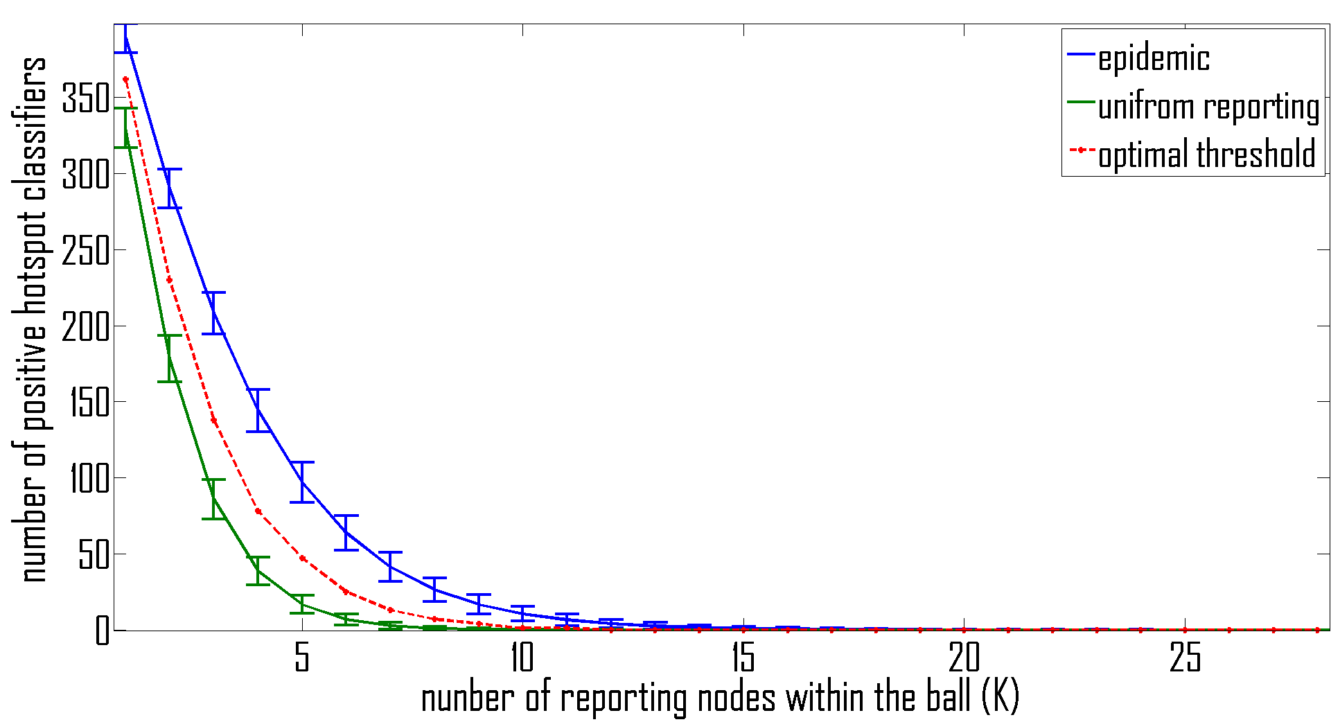
First, we considered idenfitiability on an Erd s-Renyi graph in the regime where the giant component emerges, $G(N=8000,p=2/N$) (Durrett (2010)). We performed $2000$ trials for each scenario (epidemic or uniform reporting) and evaluated the mean number of hotspots as a function of the threshold $K$ for a ball of a given radius. The resulting graph for a ball of radius $l=3$ is presented in Fig. C.1, including the corresponding standard deviations. The graph shows that, as our theory predicts, the number of hotspots is indeed a strong statistic for distinguishing between an epidemic and a random illness. This was followed, as described in the paper, by evaluating the algorithm performance in the acute regime, where the number of false positives and false negatives each tends to infinity (Fig. 5.1). In this figure, the infection size is $O(N^{0.3})$ while the reporting probability is $O(N^{-0.2}$). The ratio of false positives to true positives is $O(N^{0.3})$. The mean error is the average of the type I and type II error probabilities, assuming equal likelihoods of an epidemic and a uniform reporting event. The plot was obtained by Monte Carlo simulations of $2000$ trials for each scenario.

We have followed suit and applied the algorithm on real world networks. In Fig. C.2 the algorithm’s error rate on a subgraph of the Facebook network is presented. Even though the noise level is extremely high and the infection is tiny, the error rate is negligible. We have also simulated our algorithm on the Internet autonomous system (AS) network, in order to examine whether this algorithm is able to detect failure cascades of BGP routers (Fig. C.3). In both cases, as discussed in Section 5, the algorithm showed very good results, even for the large ball radius $l=4$. These results were obtained in a challenging setting, under a highly noisy environment with multiple epidemic sources, where only a mere fraction of the nodes truly report. In both cases, the Median Ball algorithm’s error was close to $0.5$, almost as high as a random classifier. While in principle this algorithm might be modified to include multiple seeds, this modification requires knowledge of seed number, which is rarely known. In addition, if the Median Ball algorithm are modified, the type I error increases appreciably.

Figure C.2: The error probability as a function of the number of epidemic sources on a Facebook graph. The algorithm with ball radii $r=1,2,3$ correctly classified every one of the $4000$ samples, and the error rate for the ball with radius $r=4$ is low as well. The infected component is composed of only $3\%$ of the entire graph. The number of truly reporting nodes is a mere $0.3\%$ of the graph. Finally, for each truly reporting node there are $8$ false positives ($f=8$).

Figure C.3: The error probability as a function of number of epidemic sources on the Internet AS graph. The Internet is well known for its ultra small world property, and the mean distance between nodes is less than four. The best results are achieved using balls of either $r=2$ or $r=3$ radius. The number of infected nodes is $6.7\%$ of the $27K$ ASs composing the internet. The reporting probability is $q=0.05$ so only $0.3\%$ of the nodes in the graph are truly reporting. Finally, for each truly reporting node there are $8$ false positives ($f=8$).

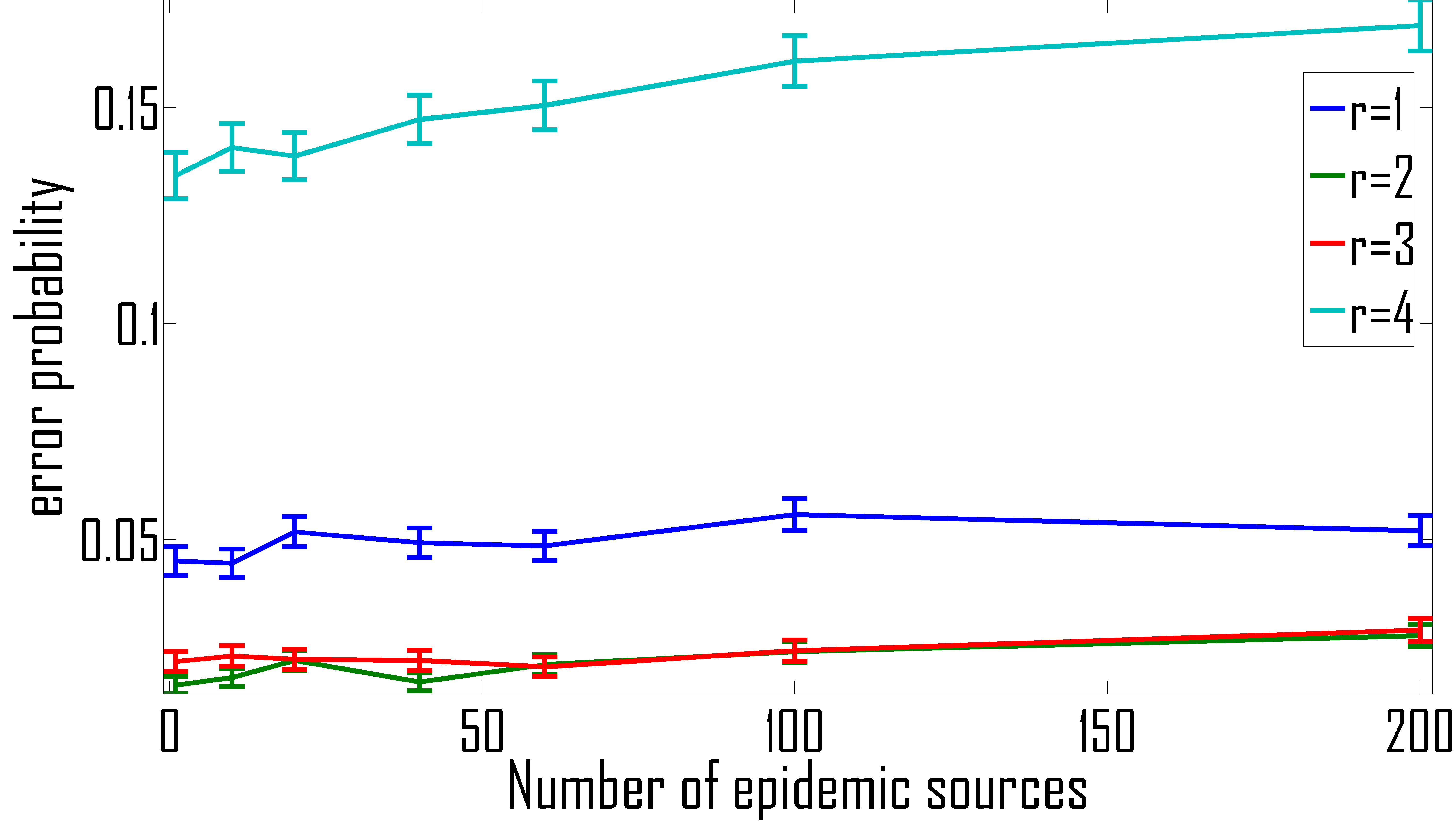
The degree distribution of these networks closely resembles power law. In particular, the degree distribution of most of this networks is $Ax^{\alpha}$ with $3>\alpha>2$. We have tested our algorithm on random power law (Fig. C.4). As the number of reporting nodes increases, there are more positive classifiers in the uniform reporting scenario. In order to compensate for this effect, one needs to design a classifier for less frequent events. This is done by increasing the threshold $K$, which in turn increases the rarity of the event. Indeed, it is possible to achieve low error rates with small ball radii even in the presence of a large number of false positives.

Figure C.4: The error probability as a function of the number of uniformly reporting nodes to truly reporting nodes $(f)$ in a scale free network. The number of false positives is approximately $f/\left(f+1\right)$. The plot was generated using Monte Carlo simulation on a scale free network of $N=8.4K$ nodes. There are roughly $0.4N$ infected nodes, whereas only $0.1N$ nodes report their infectious state. The degree distributation is $\Pr\left(deg(i)=x\right)=Ax^{-2.5}.$

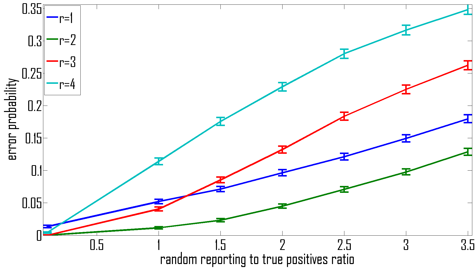
While it is often clearer to state the proofs by means of the border set, it is often simpler to implement the algorithm in terms of a local ball environment. Recall the definition of the radius-$l$ ball ball indicator

$$H_{i}^{B}(l,s)=\begin{cases}1&\left|\{v\in B_{i}(l)\cap S\}\right|\geq s\\ 0&\text{otherwise}\end{cases}.$$

As the number of nodes in a ball may vary, and due to finite size effects, the optimal threshold value $T$ may be different than the corresponding theoretical value. In practice, one may optimize this threshold value in an independent preprocessing step. In practice, values close to the theoretical predictions were found adequate in most cases.

References

- Auerbach et al. (1984) Auerbach, D M, Darrow, W W, Jaffe, H W, and Curran, J W. Cluster of cases of the acquired immune deficiency syndrome. Patients linked by sexual contact. The American journal of medicine, 76(3):487–92, March 1984. ISSN 0002-9343.
- Blair-Stahn (2010) Blair-Stahn, Nathaniel D. First passage percolation and competition models. pp. 24, May 2010.
- Cohen & Havlin (2003) Cohen, Reuven and Havlin, Shlomo. Scale-Free Networks Are Ultrasmall. Physical Review Letters, 90(5):058701, February 2003. ISSN 0031-9007. doi: 10.1103/PhysRevLett.90.058701.
- (4) Demiris, N and O’neill, PD. Bayesian inference for epidemics with two levels of mixing. Scandinavian journal of statistics, 2005.
- Durrett (2010) Durrett, Rick. Random Graph Dynamics (Cambridge Series in Statistical and Probabilistic Mathematics). Cambridge University Press, 2010. ISBN 0521150167.
- Ganesh et al. (2005) Ganesh, A., Massoulie, L., and Towsley, D. The effect of network topology on the spread of epidemics. In Proceedings IEEE 24th Annual Joint Conference of the IEEE Computer and Communications Societies., volume 2, pp. 1455–1466. IEEE, 2005. ISBN 0-7803-8968-9. doi: 10.1109/INFCOM.2005.1498374.
- Gopalan et al. (2011) Gopalan, Aditya, Banerjee, Siddhartha, Das, Abhik K., and Shakkottai, Sanjay. Random mobility and the spread of infection. In 2011 Proceedings IEEE INFOCOM, pp. 999–1007. IEEE, April 2011. ISBN 978-1-4244-9919-9. doi: 10.1109/INFCOM.2011.5935329.
- Janson (2004) Janson, Svante. Large deviations for sums of partly dependent random variables. Random Structures and Algorithms, 24(3):234–248, May 2004. ISSN 1042-9832. doi: 10.1002/rsa.20008.
- Karamchandani & Franceschetti (2013) Karamchandani, Nikhil and Franceschetti, Massimo. Rumor source detection under probabilistic sampling. In 2013 IEEE International Symposium on Information Theory, pp. 2184–2188. IEEE, July 2013. ISBN 978-1-4799-0446-4. doi: 10.1109/ISIT.2013.6620613.
- (10) Klimt, B and Yang, Y. The enron corpus: A new dataset for email classification research. Machine learning: ECML 2004, 2004.
- Milling et al. (2012) Milling, Chris, Caramanis, Constantine, Mannor, Shie, and Shakkottai, Sanjay. Network forensics. In Proceedings of the 12th ACM SIGMETRICS/PERFORMANCE joint international conference on Measurement and Modeling of Computer Systems - SIGMETRICS ’12, volume 40, pp. 223, New York, New York, USA, June 2012. ACM Press. ISBN 9781450310970. doi: 10.1145/2254756.2254784.
- Milling et al. (2013) Milling, Chris, Caramanis, Constantine, Mannor, Shie, and Shakkottai, Sanjay. Detecting epidemics using highly noisy data. In Proceedings of the fourteenth ACM international symposium on Mobile ad hoc networking and computing - MobiHoc ’13, pp. 177, New York, New York, USA, July 2013. ACM Press. ISBN 9781450321938. doi: 10.1145/2491288.2491294.
- (13) Shah, D and Zaman, T. Detecting sources of computer viruses in networks: theory and experiment. ACM SIGMETRICS Performance Evaluation Review, 2010.
- (14) Streftaris, G and Gibson, GJ. Statistical inference for stochastic epidemic models. …17th Int’l Workshop on Statistical Modelling. …, 2002.
- Viswanath et al. (2009) Viswanath, Bimal, Mislove, Alan, Cha, Meeyoung, and Gummadi, Krishna P. On the evolution of user interaction in Facebook. In Proceedings of the 2nd ACM workshop on Online social networks - WOSN ’09, pp. 37, New York, New York, USA, August 2009. ACM Press. ISBN 9781605584454. doi: 10.1145/1592665.1592675.
- Watts & Strogatz (1998) Watts, D J and Strogatz, S H. Collective dynamics of ’small-world’ networks. Nature, 393(6684):440–2, June 1998. ISSN 0028-0836. doi: 10.1038/30918.