A Complete Atlas of H I Absorption toward H II Regions
in the Southern Galactic Plane Survey (SGPS I)

Abstract

We present a complete catalog of H I emission and absorption spectrum pairs, toward H II regions, detectable within the boundaries of the Southern Galactic Plane Survey (SGPS I), a total of 252 regions. The catalog is presented in graphical, numerical and summary formats. We demonstrate an application of this new dataset through an investigation of the locus of the Near 3kpc Arm.

1 Introduction

Combining data from the Australia Telescope Compact Array (ATCA) and the Parkes single dish telescopes, the SGPS (SGPS, McClure-Griffiths et al., 2005) provides H I line and 1.4 GHz radio continuum data for the fourth Galactic quadrant, with the best combination of resolution and sensitivity currently available for that line in this area. Using these data, we have measured 21-cm absorption spectra toward a sample of 252 H II regions.

This study produces two distinct data products: a consolidated census of H II regions with known radio recombination line (RRL) velocities, taken from the literature; as well as the H I emission and absorption spectrum pairs towards them - within the bounds of the SGPS (255°$<l<$353°). These two resources will enable further study into the structure and dynamics of the neutral interstellar medium (ISM) in the fourth quadrant (on which massive stars and their formation have a significant impact). The catalogs will serve as a data set for numerous studies; including investigations of the spiral structure of the Galaxy (eg. Strasser et al., 2007) and kinematic distance works, both for target regions (eg. Urquhart et al., 2012) as well as for the intervening H I clouds (eg. Roman-Duval et al., 2009).

The sample selection from existing H II region catalogs is described in Section 2, while the method of spectrum extraction appears in Section 3. The catalog itself appears in Section 4, before a disucssion of the global properties of H I absorption in Section 5 and an illustration of its use: an examination of the distribution of H I absorption in longitude-velocity ($lv$) space, including the locus of the Near 3kpc Arm.

2 Data

2.1 Southern Galactic Plane Survey, SGPS

The Southern Galactic Plane Survey covers 325 square degrees of the Galactic plane over the fourth and first Galactic quadrants (SGPS I and SGPS II respectively). For this work, SGPS refers to the fourth quadrant component of the survey only (i.e. the SGPS I). The SGPS I provides both the H I line data, as well as the continuum maps (Haverkorn et al., 2006) used for source detection and identification.

The SGPS provides three distinct data products: Parkes continuum-subtracted cubes, with an angular resolution of $15\arcmin$; combined Parkes and Australia Telescope Compact Array (ATCA) continuum-subtracted H I cubes (2.′2) and combined Parkes and ATCA cubes containing continuum emission ($\sim 1.\arcmin 6$). For this work we use the continuum included combined Parkes-ATCA data. These cubes were specifically produced for H I absorption studies, as they provide accurately calibrated data at the highest angular resolution of the SGPS. All SGPS continuum and line cube data is available online via the Australia Telescope National Facility (ATNF) H I Surveys archive .

SGPS data has been used extensively in a number of fields, including H I self-absorption (Gibson et al., 2005; Kavars et al., 2005), the cold neutral interstellar medium in the outer Galaxy (Strasser et al., 2007), Galactic structure (McClure-Griffiths et al., 2004) as well as investigations of particular individual sources (Kothes & Dougherty, 2007).

2.2 H II Regions

Firstly we compiled a list of H II regions from RRL catalogs for the longitude and latitude range of the SGPS. This compilation of H II regions was then over-plotted on the SGPS radio continuum maps using the KARMA software suite (Gooch, 1995). Each map was then visually inspected to confirm H II region detection. Target H II regions were included in this catalog (§4) if a single, distinct emission source was visible in the SGPS continuum map.

Several cataloged H II regions were coincident with several radio continuum sources and some targets had coordinates coincident with no continuum source. It is not surprising that the SGPS with angular resolution of $\sim 2\arcmin$ detects multiple sources within the larger beam of the early H II region discovery works, for instance the Parkes beam of Caswell & Haynes (1987) is $\sim 4\arcmin$. Furthermore, there are often clusters of continuum emission sources surrounding a cataloged region’s coordinates, such that no attempt can be made to distinguish the background emission (see §3). There are several H II regions that are included in more than one H II region RRL velocity catalog (§2.2.1) and therefore become duplicate sources when the catalogs are combined. Furthermore, there were H II regions that did not appear as continuum sources in the SGPS, or had continuum temperatures $T_{\rm{cont}}<5$K, these were not included in this catalog.

The total number of individual, distinct H II regions, visible in the SGPS continuum is 252. Throughout this work, the name (in form “G longitude $\pm$latitude”) reported for each H II region is taken from the catalog from which the region is provided (see §2.2.1); hence the inconsistencies in decimal precision.

2.2.1 H II Region Catalogs

We use the catalog of Caswell & Haynes (1987) as the basis of our target list, supplementing that catalog with further H II regions sourced from other works. Our final source list is a compilation of the H II region RRL velocity catalogs of Caswell & Haynes (1987), the Green Bank Telescope H II Region Discovery Survey (Bania et al., 2010), Lockman (1989) and Wilson et al. (1970) (see Table 4). We describe each of these works below.

There are several other fourth quadrant studies which include H II region candidates (Reifenstein et al., 1970; Walsh et al., 1999; Busfield et al., 2006; Urquhart et al., 2012; Foster et al., 2011), but as Hn$\alpha$ emission has not been detected towards these candidates, they are not confirmed H II regions and are therefore excluded from this work.

Caswell & Haynes (1987)

Hydrogen RRL parameters for 316 H II regions, observed with the Parkes 64-m Radio Telescope, over the longitude range $210\arcdeg<l<360\arcdeg$ are provided by Caswell & Haynes (1987). The majority of H II regions in this study were sourced from this work, the southern correspondent to the Lockman (1989) catalog. Several of the H II regions cataloged by Caswell & Haynes (1987) are outside the bounds of the SGPS; therefore for regions with Galactic longitudes $l<245\arcdeg$, or $l>353\arcdeg$, or Galactic latitudes $|b|\gtrsim 1.4\arcdeg$ we cannot extract H I E/A spectra (and they are not included in this catalog).

Green Bank Telescope H II Region Discovery Survey

The Green Bank Telescope H II Region Discovery Survey (GBTHRDS, Bania et al., 2010) detected 602 RRL components towards 448 continuum sources in the Galactic plane between $344\arcdeg<l<67\arcdeg$. The survey more than doubled the number of known H II regions within that longitude range - the majority of previously known H II regions were sourced from the Lockman (1989) catalog, see below. With a 95% detection rate the GBTHRDS selected its target sample from spatially coincident mid-infrared and radio continuum emission. The Spitzer MIPSGAL survey (Carey et al., 2009) provided 24$\mu$m data, while 21cm continuum emission was sourced from the SGPS, VGPS (Stil et al., 2006) and NVSS (Condon et al., 1998).

Lockman (1989)

The canonical northern hemisphere catalog of Lockman (1989) extends into the fourth quadrant, and therefore into the SGPS coverage area. This large survey provides RRL velocity detections for 462 H II regions.

Wilson et al. (1970)

Wilson et al. (1970) detected the H$109\alpha$ RRL toward 130 H II regions visible in the southern sky ($261\arcdeg<l<50\arcdeg$) using the Parkes Radio Telescope in 1968.

3 Emission/Absorption Method of H I Absorption Spectrum Extraction

The Emission/Absorption (E/A) method observes H I spectra coincident with, and adjacent to, discrete continuum sources. In order to derive absorption, $e^{-\tau}$, the brightness temperature as a function of velocity, $V$, both on ($T_{\rm{on}}$) and off the source (i.e. the emission spectrum, $T_{\rm{off}}$) are compared. The simplest radiative transfer situation gives:

$$T_{\rm{on}}(V)=(T_{\rm{bg}}+T_{\rm{cont}})e^{-\tau(V)}+T_{\rm{s}}(V)(1-e^{-\tau(V)})$$ (1)

$$T_{\rm{off}}(V)=T_{\rm{bg}}e^{-\tau(V)}+T_{\rm{s}}(V)(1-e^{-\tau(V)})$$ (2)

where $T_{\rm{cont}}$ is the continuum source brightness temperature, $T_{\rm{s}}$ is the spin temperature of the foreground cloud(s) and $T_{\rm{bg}}$ represents the brightness temperature of any other background contribution (see Figure 1).

Assuming that the ‘on’ and ‘off’ spectra both sample the same gas, subtraction of one from the other removes the common $T_{\rm{bg}}$ and $T_{\rm{s}}(V)$ terms, allowing the absorption to be calculated directly,

$$e^{-\tau}=\frac{T_{\rm{on}}-T_{\rm{off}}}{T_{\rm{cont}}}$$ (3)

The ‘on’ and three ‘off’ source positions, which were averaged to provide an emission estimate, were chosen in accordance with the criteria identified in Jones & Dickey (2012). Large scale H I emission fluctuations, which are present on all angular scales (Green, 1993; Dickey et al., 2001), are reflected by the variation in the three ‘off’ source positions, see §3.2. The E/A method is described in detail by Kolpak et al. (2003).

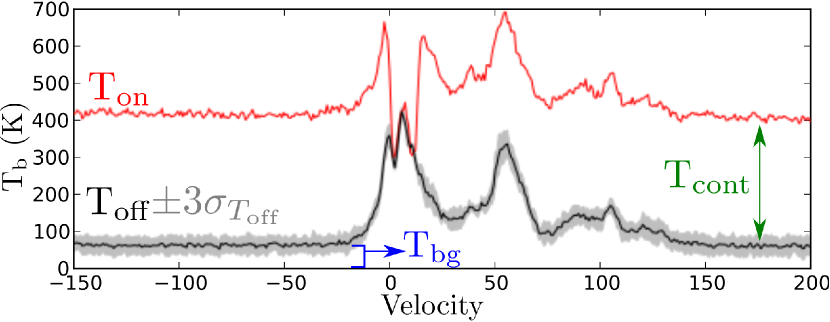
Figure 1: Brightness temperature of sample $T_{\rm{on}}$ (peak brightness, shown in red) and average off source (black) spectra for G269.133-1.137. The grey envelope around the average off source spectrum represents a $3\sigma$ variation between the three off source positions. Components of Equations 1 and 2 are labeled. (A color version of this figure is available in the online journal.)

3.1 Continuum Calibration

The continuum temperature is estimated from the difference in on and off spectra across a range of velocity channels in which there is no H I signal. For most spectra we used the velocity channel range 100km s^-1 $<V<175$km s^-1 as this avoids both expected Galactic circular rotation velocities as well as avoiding the ends of the spectrum band.

The SGPS line data is recorded in units Jy/beam, therefore a conversion to K is required. Firstly a two-dimensional Gaussian beam solid angle is assumed (Equation 4), then the flux density for an unresolved source is approximated (Equation 5) in terms of antenna temperature.

$$\Omega=\frac{\pi}{4\ln(2)}(\rm{FWHM}_{\phi}\times\rm{FWHM}_{\psi})$$ (4)

$$S=\frac{2k}{\lambda^{2}}\Omega T_{A}$$ (5)

Theoretically, the antenna temperature is the convolution of the beam response with the sky brightness temperature distribution, integrated over the entire sky. Substituting for beam solid angle, $\lambda=21.1$cm and creating dimensionless variables results in Equation 6.

$$T_{b}\approx 606\frac{S/\rm{(Jy/beam)}}{(\rm{FWHM}_{\psi}\times\rm{FWHM}_{\phi})/arcseconds^{2}}\qquad\rm{K}$$ (6)

The dimensions of each synthesized beam are given in Table 4 of McClure-Griffiths et al. (2005).

This conversion factor is used to convert the brightness temperature of the off source spectrum (top panel) of each image in Figure 4 as well as to obtain the continuum temperature reported in Table 4. However, the conversion is $not$ required in the calculation of absorption (see Equation 3).

3.2 Quality of Spectra

As for most emission/absorption studies, the noise level in the absorption spectrum is not dictated by radiometer noise, but rather the precision with which the absorption spectrum can be subtracted from background continuum emission, see Equation 3 (Dickey et al., 2003).

A series of five tests were devised to measure the quality of each H I absorption spectrum (see Figure 2)—resulting in six quality categories A-F. The quality category for each spectrum included in the catalog is given in Table 4. Each spectrum was initially assumed to be at the best quality rating (i.e. category A); the quality factor was then down-graded for each test failed; therefore the spectra in category F failed all five quality tests listed below.

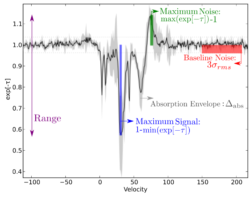
Figure 2: Sample absorption spectrum for G254.676+0.229, $e^{-\tau}$ is the solid black line, demonstrating the quality tests. The range (puprle), maximum signal (blue) and maximum noise (green), baseline noise (red) and absorption fluctuation envelope (grey) are shown. (A color version of this figure is available in the online journal.)

Range

Tests if the range of calculated absorption values are realistic: theoretically $0<e^{-\tau}<1$. Continuum temperature uncertainties or uncertainties in assumed background emission spectrum will increase the range of $e^{-\tau}$. This test is failed if Range($\exp[-\tau]$)$>1.5$.

Maximum Signal to Maximum Noise

‘Maximum signal’ refers to $1-min(\exp[-\tau])$ and ‘maximum noise’ refers to $max(\exp[-\tau])-1$, see Figure 2. This test is designed to ascertain if emission signals (which should have been removed) overwhelm absorption in the spectrum. This test is failed if (maximum signal/maximum noise)$<3$.

Absorption Uncertainty Envelope

This test investigates the fluctuations in the absorption envelope (caused by differences between the three emission, off source, spectra). The absorption uncertainty envelope is calculated as follows:

$$\Delta_{\textrm{abs}}(v)=\left|e^{-\tau}-\left(\frac{T_{\rm{on}}-(T_{\rm{off}}+3\sigma_{T_{\rm{off}}})}{T_{\rm{cont}}}\right)\right|$$ (7)

Where $\sigma_{T_{\textrm{off}}}$ is the standard deviation between the three emission spectra, for each velocity channel. This test is failed if the standard deviation of this envelope, over the whole velocity range, is large: i.e. $3\sigma(\Delta_{\rm{abs}})>1$. The absorption uncertainty envelope is shown as grey shading in each H I absorption spectrum panel (see Figures 2 and 4), while $\pm 3\sigma_{T_{\rm{off}}}$ is shown as the grey shading in each H I emission spectrum panel (Figure 4).

Baseline Noise

This test identifies absorption spectra with high levels of baseline noise. This is achieved by investigating the standard deviation of absorption ($\sigma_{\rm{rms}}$) over the same velocity channel range from which the continuum temperature is determined, i.e. there is no H I emission nor absorption signals (see §3.1). This test is failed if $3\sigma_{\rm{rms}}>1$.

Number of Velocity Channels with Significant Absorption

The final test is a count of the number of velocity channels which demonstrate statistically significant amounts of absorption. That is, the absorption is deeper than a combination of the baseline noise and the absorption envelope uncertainty: $e^{-\tau}(v)<(1-3\sigma_{\rm{rms}}-\sigma(\Delta_{\rm{abs}}))$ . At least 15 channels of statistically significant absorption are required to pass this test. Note that $\sigma(\Delta_{\rm{abs}})\propto 3\sigma_{T_{\rm{off}}}$ (see Absorption Uncertainty Envelope test).

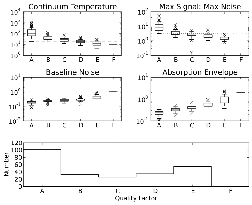
Figure 3: Assessment of the quality control variables for each H I absorption spectrum in categories A (best quality) to F (poorest quality). In each panel, the horizontal dotted line signifies the value for which the test is failed (see text). The distribution of continuum temperatures in each quality category is also shown, even though contintuum temperatures do not constitute a formal quality test (§3.2); in this case the dashed horizontal line demonstrates the limit in continuum temperature required for resolution of the kinematic distance ambiguity from Jones & Dickey (2012). The bottom panel displays a histogram of the number of H II regions in each quality category. (A color version of this figure is available in the online journal.)

The majority of the poorest quality spectra (category F) come from target regions with $l>340\arcdeg$ and were usually sourced from the H II region catalog of the GBTHRDS. This is not particularly surprising as the GBTHRDS avoided previously-observed H II regions; resulting in intrinsically fainter sources compared to Caswell & Haynes (1987).

The bottom panel of Figure 3 displays the number of regions in each quality category. The distribution appears to be superficially bimodal, such that the quality categories could be regrouped into ‘good’ and ‘poor’ umbrella categories associated with quality factors A-C and D-F respectively. Through the use of these umbrella categories it can be shown that in order to extract a ‘good’ quality H I absorption spectrum, a continuum temperature greater than $\sim 20$K is required—note: while continuum temperature was not used as a quality assurance paramater, stronger sources are associated with higher quality factors (see Figure 3).

Jones & Dickey (2012) reported that a continuum temperature of at least 10K is required to solve the kinematic distance ambiguity for H II regions in the SGPS, using their velocity channel summation technique. This limit approximately corresponds to the median continuum temperature of quality category E (10.4 K). Note that H II regions with continuum temperatures $T_{\rm{cont}}<5$ K were not included in the catalog of H I spectra (§2.2).

4 Catalog

The catalog of H I emission/absorption spectrum pairs is the primary data product of this work. We present it here in three formats: individual spectrum figures, complete data set (in tar format) and summary table.

Catalog Summary

Table 4 provides an overview of the entire catalog. The 252 included H II regions are listed, along with their known parameters. The columns list the Galactic coordinates of the H II region (as reported by the original reference); SIMBAD identification; $T_{\rm{cont}}$ (K), quality factor, RRL velocity and RRL velocity reference respectively.

Table 1: H II Region Catalog

Longitude	Latitude	SIMBAD ID	Tcont	Qual	VRRL	Ref
254.676	$+$0.299	NGC 2579 (catalog )	A	134	64	1
263.619	$-$0.533	GAL 263.62-00.53 (catalog )	A	58	1	1
267.947	$-$1.066	GAL 267.95-01.07 (catalog )	A	969	1	1
268.0	$-$1.1	GAL 268.0-01.1 (catalog )	B	31	1.8	4
268.454	$-$0.848	GAL 268.45-00.85 (catalog )	A	94	5	1
269.133	$-$1.137	GAL 269.13-01.14 (catalog )	A	118	15	1
270.294	$+$0.848	GAL 270.29+00.85 (catalog )	E	26	1	1
274.013	$-$1.141	GUM 26 (catalog )	A	317	39	1
281.595	$-$0.969	GAL 281.60-00.97 (catalog )	C	30	2	1
282.026	$-$1.181	GAL 282.03-01.18 (catalog )	A	235	19	1
282.632	$-$0.853	GAL 282.63-00.85 (catalog )	E	12	0	1
283.131	$-$0.984	GAL 283.13-00.98 (catalog )	D	35	$-$1	1
283.312	$-$0.566	GAL 283.31-00.57 (catalog )	E	20	6	1
283.329	$-$1.050	GAL 283.33-01.05 (catalog )	C	26	16	1
284.308	$-$0.334	GUM 29 (catalog )	A	879	0	1
284.559	$-$0.183	GAL 284.56-00.18 (catalog )	B	29	9	1
284.650	$-$0.484	GAL 284.65-00.48 (catalog )	E	17	5	1
284.723	$+$0.313	GAL 284.72+00.31 (catalog )	A	72	10	1
285.253	$-$0.053	GAL 285.25-00.05 (catalog )	A	321	$-$2	1
286.195	$-$0.163	GAL 286.20-00.16 (catalog )	A	52	$-$18	1
286.873	$-$0.883	GAL 286.87-00.88 (catalog )	D	24	$-$20	1
287.217	$+$0.053	GAL 287.22+00.05 (catalog )	E	29	$-$25	1
287.247	$+$0.355	GAL 287.25+00.36 (catalog )	E	22	$-$18	1
287.393	$-$0.630	GAL 287.39-00.63 (catalog )	A	415	$-$17	1
287.550	$-$0.616	GAL 287.55-00.62 (catalog )	A	344	$-$39, -14	1
289.063	$-$0.355	GAL 289.06-00.36 (catalog )	A	88	19	1
289.755	$-$1.152	GUM 35 (catalog )	B	38	22	1
289.878	$-$0.792	2MASX J11005954-6050229 (catalog )	A	50	22	1
290.646	$+$0.256	GAL 290.65+00.26 (catalog )	D	10	$-$28	1
291.059	$-$0.770	GAL 291.06-00.77 (catalog )	B	41	17	1
291.284	$-$0.713	OH 291.3 -0.7 (catalog )	A	1377	$-$25	1
291.466	$-$0.128	GAL 291.47-00.13 (catalog )	E	22	6	1
291.858	$-$0.675	GAL 291.86-00.68 (catalog )	A	84	25	1
293.027	$-$1.031	GAL 293.03-01.03 (catalog )	D	18	66	1
295.760	$-$0.200	GAL 295.76-00.20 (catalog )	E	5	17	1
296.593	$-$0.975	GAL 296.59-00.98 (catalog )	E	8	25	1
297.506	$-$0.765	GAL 297.51-00.77 (catalog )	B	45	23	1
297.655	$-$0.977	GAL 297.66-00.98 (catalog )	B	41	26	1
298.187	$-$0.782	GAL 298.19-00.78 (catalog )	B	14	16	1
298.228	$-$0.331	GAL 298.23-00.33 (catalog )	A	84	31	1
298.868	$-$0.432	GAL 298.87-00.43 (catalog )	A	417	25	1
299.016	$+$0.148	GAL 299.02+00.15 (catalog )	D	15	23	1
299.363	$-$0.257	GAL 299.36-00.26 (catalog )	D	24	$-$37	1
300.479	$-$0.192	GAL 300.48-00.19 (catalog )	C	20	26	1
300.956	$+$1.161	GUM 43 (catalog )	A	60	$-$47	1
301.109	$+$0.969	GAL 301.11+00.97 (catalog )	A	119	$-$42	1
301.814	$+$1.077	GAL 301.81+01.08 (catalog )	E	11	$-$42	1
302.025	$-$0.044	GAL 302.03-00.04 (catalog )	A	19	$-$27	1
302.504	$-$0.749	GAL 302.69+00.19 (catalog )	D	19	31	1
302.690	$+$0.190	WR 47b (catalog )	E	13	$-$33	1
302.804	$+$1.306	GAL 302.80+01.31 (catalog )	D	8	$-$32	1
305.173	$-$0.368	GAL 305.17-00.37 (catalog )	E	20	$-$45	1
305.202	$+$0.022	GAL 305.20+00.02 (catalog )	A	241	$-$40	1
305.363	$+$0.179	GAL 305.36+00.18 (catalog )	A	513	$-$38	1
305.537	$+$0.338	GAL 305.54+00.34 (catalog )	C	72	$-$39	1
305.551	$-$0.005	GAL 305.55-00.01 (catalog )	A	117	$-$45	1
305.787	$+$0.140	GAL 305.79+00.14 (catalog )	E	11	$-$43	1
306.256	$+$0.066	GAL 306.26+00.07 (catalog )	E	7	$-$37	1
306.315	$-$0.361	GAL 306.32-00.36 (catalog )	B	40	$-$16	1
307.569	$-$0.616	GAL 307.57-00.62 (catalog )	D	21	$-$40	1
307.620	$-$0.320	GAL 307.62-00.32 (catalog )	A	76	$-$37	1
308.092	$-$0.432	GAL 308.09-00.43 (catalog )	E	21	$-$17	1
308.647	$+$0.579	GAL 308.65+00.58 (catalog )	A	42	$-$50	1
309.057	$+$0.186	GAL 309.06+00.19 (catalog )	E	12	$-$47	1
309.548	$-$0.737	GAL 309.55-00.74 (catalog )	C	35	$-$43	1
309.905	$+$0.373	GAL 309.91+00.37 (catalog )	B	36	$-$55	1
310.176	$-$0.131	GAL 310.18-00.13 (catalog )	E	16	4	1
310.796	$-$0.408	NAME Kes 20A (catalog )	D	17	33,-57	1
310.994	$+$0.389	GAL 310.99+00.39 (catalog )	E	11	$-$51	1
311.114	$-$0.270	GAL 311.11-00.27 (catalog )	C	24	36	1
311.197	$+$0.752	GAL 311.20+00.75 (catalog )	C	19	$-$57	1
311.489	$+$0.368	IRAS 14000-6104 (catalog )	C	39	$-$59	1
311.497	$-$0.483	GAL 311.50-00.48 (catalog )	D	27	$-$47	1
311.627	$+$0.270	GAL 311.63+00.27 (catalog )	B	43	$-$61	1
311.852	$-$0.222	GAL 311.85-00.22 (catalog )	D	11	$-$55	1
311.894	$+$0.100	[CH87] 311.894+0.100 (catalog )	A	104	$-$47	1
311.922	$+$0.229	GAL 311.92+00.23 (catalog )	A	76	$-$45	1
312.112	$+$0.314	PN G312.1+00.3 (catalog )	A	42	$-$49	1
312.953	$-$0.449	GAL 312.95-00.45 (catalog )	D	20	$-$47	1
313.446	$+$0.176	GAL 313.45+00.18 (catalog )	B	26	$-$5	1
314.228	$+$0.437	GAL 314.23+00.44 (catalog )	A	66	$-$63	1
315.312	$-$0.273	GAL 315.31-00.27 (catalog )	D	10	16	1
316.156	$-$0.492	GAL 316.16-00.49 (catalog )	A	35	$-$60	1
316.393	$-$0.356	GAL 316.39-00.36 (catalog )	C	19	3	1
316.808	$-$0.037	GAL 316.81-00.04 (catalog )	A	462	$-$36	1
317.037	$+$0.300	GAL 317.04+00.30 (catalog )	C	40	$-$49	1
317.291	$+$0.268	GAL 317.29+00.27 (catalog )	D	23	$-$51	1
317.598	$-$0.363	GAL 317.60-00.36 (catalog )	E	17	$-$38	1
317.988	$-$0.759	GAL 317.99-00.76 (catalog )	E	13	$-$37	1
318.058	$-$0.459	IRAS 14518-5925 (catalog )	E	10	$-$31,37	1
318.911	$-$0.181	GAL 318.91-00.18 (catalog )	A	41	$-$29	1
319.157	$-$0.423	GAL 319.16-00.42 (catalog )	A	49	$-$22	1
319.380	$-$0.025	GAL 319.38-00.03 (catalog )	A	91	$-$14	1
319.874	$+$0.770	GAL 319.87+00.77 (catalog )	A	35	$-$38	1
320.109	$-$0.510	[CH87] 320.109-0.510 (catalog )	D	16	$-$13	1
320.153	$+$0.780	GAL 320.15+00.78 (catalog )	A	170	$-$36	1
320.236	$+$0.417	GAL 320.24+00.42 (catalog )	B	31	$-$31	1
320.252	$-$0.332	GAL 320.25-00.33 (catalog )	A	92	$-$68	1
320.317	$-$0.208	GAL 320.32-00.21 (catalog )	A	120	$-$11	1
320.379	$+$0.139	GAL 320.38+00.14 (catalog )	B	30	$-$3	1
320.706	$+$0.197	GAL 320.71+00.20 (catalog )	D	20	$-$7	1
321.038	$-$0.519	GAL 321.04-00.52 (catalog )	A	111	$-$61	1
321.105	$-$0.549	GAL 321.11-00.55 (catalog )	A	60	$-$56	1
321.710	$+$1.157	GAL 321.71+01.16 (catalog )	A	38	$-$32	1
322.153	$+$0.613	GAL 322.15+00.61 (catalog )	A	281	$-$52	1
322.407	$+$0.221	GAL 322.41+00.22 (catalog )	C	14	$-$30	1
324.120	$-$0.954	GAL 324.12-00.95 (catalog )	E	6	$-$67	1
324.147	$+$0.231	[CH87] 324.147+0.231 (catalog )	C	31	$-$91	1
324.192	$+$0.109	[CH87] 324.192+0.109 (catalog )	A	53	$-$92	1
324.954	$-$0.584	[CH87] 324.954-0.584 (catalog )	E	10	25	1
326.141	$-$0.328	[CH87] 326.141-0.328 (catalog )	E	9	$-$65	1
326.230	$+$0.976	[CH87] 326.230+0.976 (catalog )	E	10	$-$42	1
326.441	$+$0.914	[CH87] 326.441-0.396 (catalog )	A	161	$-$39	1
326.645	$+$0.589	[DBS2003] 95 (catalog )	A	425	$-$44	1
326.959	$+$0.031	GAL 326.96+00.03 (catalog )	C	30	$-$64	1
327.313	$-$0.536	[CH87] 327.313-0.536 (catalog )	A	722	$-$48	1
327.612	$-$0.354	[CH87] 327.612-0.354 (catalog )	B	46	$-$72	1
327.759	$-$0.351	[CH87] 327.759-0.351 (catalog )	A	68	$-$72	1
327.834	$+$0.113	[CH87] 327.834+0.113 (catalog )	D	18	$-$100	1
327.985	$-$0.086	GAL 327.99-00.09 (catalog )	A	59	$-$45	1
328.310	$+$0.448	GAL 328.31+00.45 (catalog )	D	8	$-$97	1
328.593	$-$0.518	GAL 328.59-00.52 (catalog )	A	208	$-$51	1
328.806	$-$0.083	GAL 328.81-00.08 (catalog )	B	32	$-$47	1
328.812	$+$0.637	GAL 328.81+00.64 (catalog )	C	17	$-$42	1
329.353	$+$0.144	GAL 329.35+00.14 (catalog )	B	34	$-$107	1
329.489	$+$0.207	GAL 329.49+00.21 (catalog )	D	30	$-$102	1
330.041	$-$0.045	GAL 330.04-00.05 (catalog )	B	28	$-$38	1
330.305	$-$0.385	GAL 330.31-00.39 (catalog )	B	19	$-$76	1
330.677	$-$0.396	GAL 330.68-00.40 (catalog )	A	58	$-$61	1
330.856	$-$0.371	GAL 330.86-00.37 (catalog )	A	173	$-$56	1
331.026	$-$0.152	GAL 331.03-00.15 (catalog )	B	59	$-$89	1
331.110	$-$0.506	GAL 331.11-00.51 (catalog )	A	68	$-$68	1
331.259	$-$0.186	GAL 331.26-00.19 (catalog )	A	86	$-$85	1
331.314	$-$0.336	GAL 331.31-00.34 (catalog )	A	125	$-$64	1
331.353	$-$0.013	GAL 331.35-00.01 (catalog )	A	91	$-$81	1
331.354	$+$1.072	GAL 331.35+01.07 (catalog )	A	55	$-$79	1
331.360	$+$0.507	GAL 331.36+00.51 (catalog )	D	19	$-$46	1
331.517	$-$0.069	GAL 331.5-00.0 (catalog )	A	466	$-$89	1
332.148	$-$0.446	GAL 332.15-00.45 (catalog )	A	275	$-$55	1
332.541	$-$0.111	GAL 332.54-00.11 (catalog )	F	10	$-$50	1
332.662	$-$0.607	GAL 332.66-00.61 (catalog )	A	149	$-$48	1
332.978	$+$0.792	GAL 332.98+00.79 (catalog )	A	114	$-$52	1
333.114	$-$0.441	GAL 333.11-00.44 (catalog )	A	303	$-$52	1
333.168	$-$0.081	GAL 333.17-00.08 (catalog )	A	61	$-$91	1
333.292	$-$0.371	GAL 333.29-00.37 (catalog )	A	323	$-$50	1
333.6	$-$0.1	GAL 333.6-00.1 (catalog )	A	89	$-$53.7	4
333.61	$-$0.208	SNR G333.6-00.2 (catalog )	A	840	$-$46	1
333.684	$-$0.457	GAL 333.68-00.46 (catalog )	C	28	$-$50	1
334.529	$+$0.825	GAL 334.53+00.83 (catalog )	E	11	$-$77	1
334.684	$-$0.107	GAL 334.68-00.11 (catalog )	D	24	$-$32	1
334.714	$-$0.665	GAL 334.71-00.67 (catalog )	A	30	16	1
335.748	$-$0.134	GAL 335.75-00.13 (catalog )	C	47	$-$52	1
335.978	$+$0.185	GAL 335.98+00.19 (catalog )	E	24	$-$79	1
336.375	$-$0.131	GAL 336.38-00.13 (catalog )	B	49	$-$88	1
336.404	$-$0.234	GAL 336.40-00.23 (catalog )	B	73	$-$93	1
336.456	$+$0.038	GAL 336.46+00.04 (catalog )	E	22	$-$63	1
336.489	$-$0.154	GAL 336.49-00.15 (catalog )	D	42	$-$84	1
336.732	$+$0.072	GAL 336.73+00.07 (catalog )	B	122	$-$78,-112	1
336.840	$+$0.047	GAL 336.84+00.05 (catalog )	B	109	$-$79	1
336.9	$-$0.1	[HHB99] 336.934-0.146 (catalog )	B	57	$-$73.1	4
337.147	$-$0.181	GAL 337.15-00.18 (catalog )	A	287	$-$73	1
337.3	$-$0.1	[KC97c] G337.3-00.1 (catalog )	C	39		4
337.548	$-$0.304	GAL 337.55-00.30 (catalog )	E	11	$-$101	1
337.665	$-$0.048	GAL 337.67-00.05 (catalog )	C	29	$-$55	1
337.949	$-$0.476	GAL 337.95-00.48 (catalog )	A	380	$-$40	1
338.014	$-$0.121	GAL 338.01-00.12 (catalog )	B	46	$-$54	1
338.131	$-$0.173	GAL 338.13-00.17 (catalog )	A	61	$-$53	1
338.398	$+$0.164	GAL 338.40+00.16 (catalog )	A	121	$-$29	1
338.407	$-$0.238	GAL 338.41-00.24 (catalog )	A	98	2	1
338.450	$+$0.061	GAL 338.45+00.06 (catalog )	A	150	$-$37	1
338.742	$+$0.641	GAL 338.74+00.64 (catalog )	D	23	$-$62	1
338.921	$-$0.089	GAL 338.92-00.09 (catalog )	A	60	$-$40	1
338.943	$+$0.604	GAL 338.94+00.60 (catalog )	A	87	$-$63	1
339.089	$-$0.216	GAL 339.09-00.22 (catalog )	D	18	$-$120	1
339.128	$-$0.408	SNR G339.2-00.4 (catalog )	D	24	$-$37	1
339.286	$+$0.163	GAL 339.29+00.16 (catalog )	E	14	$-$71	1
339.578	$-$0.124	GAL 339.58-00.12 (catalog )	D	21	$-$30	1
339.838	$+$0.274	GAL 339.84+00.27 (catalog )	A	35	$-$19	1
339.955	$-$0.566	GAL 339.96-00.57 (catalog )	E	10	$-$89	1
340.047	$-$0.253	GAL 340.05-00.25 (catalog )	C	34	$-$52	1
340.240	$+$0.482	GAL 340.24+00.48 (catalog )	C	13	$-$62	1
340.279	$-$0.222	GAL 340.28-00.22 (catalog )	A	77	$-$43	1
340.777	$-$1.008	GAL 340.78-01.01 (catalog )	A	233	$-$25	1
341.050	$-$0.100	GAL 341.05-00.10 (catalog )	E	6	$-$38	1
341.264	$-$0.317	GAL 341.26-00.32 (catalog )	E	24	$-$38	1
341.963	$+$0.205	GAL 341.96+00.21 (catalog )	D	12	$-$8	1
342.085	$+$0.423	GAL 342.09+00.42 (catalog )	A	85	$-$65	1
342.300	$+$0.314	GAL 342.30+00.31 (catalog )	E	25	$-$122	1
342.382	$-$0.044	GAL 342.38-00.04 (catalog )	D	26	$-$13	1
345.215	$-$0.749	GAL 345.22-00.75 (catalog )	D	15	$-$18	1
345.231	$+$1.035	GAL 345.23+01.04 (catalog )	A	211	$-$9	1
345.404	$+$1.406	GAL 345.40+01.41 (catalog )	A	27	$-$15	1
345.450	$+$0.209	GAL 345.45+00.21 (catalog )	B	32	$-$13	1
345.495	$+$0.326	GAL 345.50+00.33 (catalog )	A	38	$-$20	1
345.555	$-$0.042	GAL 345.56-00.04 (catalog )	A	76	$-$6	1
345.645	$+$0.010	GAL 345.65+00.01 (catalog )	A	81	$-$10	1
345.722	$+$0.153	HRDS G345.722+0.153 (catalog )	E	6	$-$77.9	2
345.827	$+$0.041	GAL 345.83+00.04 (catalog )	B	23	$-$10	1
346.056	$-$0.021	HRDS G346.056-0.021 (catalog )	D	9	$-$76.8, -3.4	2
346.077	$-$0.056	HRDS G346.077-0.056 (catalog )	E	12	$-$84.7,-7.9	2
346.206	$-$0.071	GAL 346.21-00.07 (catalog )	C	18	$-$108	1
346.267	$+$0.128	HRDS G346.267+0.128 (catalog )	E	5	$-$32.2	2
346.530	$-$0.013	HRDS G346.530-0.013 (catalog )	E	5	0.6	2
346.539	$+$0.097	GAL 346.54+00.10 (catalog )	B	35	2	1
346.875	$+$0.328	HRDS G346.875+0.328 (catalog )	E	10	4.1	2
347.386	$+$0.266	GAL 347.39+00.27 (catalog )	E	20	$-$97	1
347.600	$+$0.211	GAL 347.60+00.21 (catalog )	E	19	$-$96	1
347.772	$+$0.131	HRDS G347.772+0.131 (catalog )	E	6	$-$88.7	2
347.893	$+$0.044	GAL 347.89+00.04 (catalog )	A	51	$-$31	1
347.918	$-$0.761	HRDS G347.918-0.761 (catalog )	E	6	6.1	2
347.964	$-$0.439	GAL 347.96-00.44 (catalog )	C	27	$-$97	1
348.061	$+$0.242	HRDS G348.061+0.242 (catalog )	E	5	0.7	2
348.148	$+$0.255	HRDS G348.148+0.255 (catalog )	E	5	$-$66.3, -1.4	2
348.225	$+$0.459	GAL 348.23+00.46 (catalog )	B	61	$-$12	1
348.231	$-$0.982	ESO 333-3 (catalog )	A	237	$-$18	1
348.557	$-$0.985	HRDS G348.557-0.985 (catalog )	E	17	$-$10.5	2
348.715	$-$1.031	GAL 348.72-01.03 (catalog )	A	562	$-$13	1
348.891	$-$0.179	HRDS G348.891-0.179 (catalog )	E	8	10.1	2
349.111	$+$0.105	GAL 349.11+00.11 (catalog )	C	33	$-$74	1
349.140	$+$0.020	GAL 349.14+00.02 (catalog )	B	81	$-$92, 17	1
349.216	$+$0.144	HRDS G349.216+0.144 (catalog )	D	11	$-$65.7	2
349.579	$-$0.68	HRDS G349.579-0.680 (catalog )	C	12	$-$19.4	2
349.84	$-$0.537	GAL 349.84-00.54 (catalog )	A	110	$-$25	1
350.004	$+$0.438	HRDS G350.004+0.438 (catalog )	E	13	$-$33.5	2
350.129	$+$0.088	GAL 350.13+00.09 (catalog )	A	143	$-$69	1
350.177	$+$0.017	HRDS G350.177+0.017 (catalog )	D	14	$-$68.9	2
350.33	$+$0.157	HRDS G350.330+0.157 (catalog )	E	11	$-$62.9	2
350.335	$+$0.107	[KC97c] G350.3+00.1 (catalog )	E	12	$-$66.1	3
350.524	$+$0.960	GAL 350.52+00.96 (catalog )	A	77	$-$10	1
350.769	$-$0.075	HRDS G350.769-0.075 (catalog )	E	5	$-$62.6	2
350.813	$-$0.019	GAL 350.81-00.02 (catalog )	A	29	$-$5	1
350.996	$-$0.577	GAL 351.00-00.58 (catalog )	E	11	$-$17	1
351.063	$+$0.662	[L89b] 351.063+00.662 (catalog )	A	150	$-$3.8	3
351.192	$+$0.708	[L89b] 351.192+00.708 (catalog )	A	224	$-$3.4	3
351.201	$+$0.483	[L89b] 351.201+00.483 (catalog )	A	157	$-$7.1	3
351.358	$+$0.666	GAL 351.36+00.67 (catalog )	A	566	$-$3	1
351.359	$+$1.014	HRDS G351.359+1.014 (catalog )	E	11	$-$8.6	2
351.467	$-$0.462	GAL 351.47-00.46 (catalog )	A	80	$-$21	1
351.601	$-$0.348	GAL 351.60-00.35 (catalog )	C	20	$-$94	1
351.617	$+$0.171	GAL 351.62+00.17 (catalog )	A	173	$-$43	1
351.641	$-$1.256	GAL 351.60-01.30 (catalog )	A	102	$-$13	1
351.662	$+$0.518	GAL 351.66+00.52 (catalog )	D	19	$-$2	1
351.691	$+$0.669	HRDS G351.691+0.669 (catalog )	B	25	3.1	2
351.694	$-$1.165	GAL 351.69-01.17 (catalog )	A	138	$-$13	1
352.398	$-$0.057	GAL 352.40-00.06 (catalog )	D	21	$-$89	1
352.521	$-$0.144	HRDS G352.521-0.144 (catalog )	B	61	$-$57.3,-38	2
352.61	$+$0.177	HRDS G352.610+0.177 (catalog )	E	13	$-$50.4	2
352.611	$-$0.172	GAL 352.61-00.17 (catalog )	B	21	$-$82	1
352.676	$+$0.148	GAL 352.68+00.15 (catalog )	E	17	$-$45	1
353.035	$+$0.748	[L89b] 353.035+00.748 (catalog )	C	44	$-$9.1	3
353.136	$+$0.660	GAL 353.14+00.66 (catalog )	A	162	$-$4	1
353.186	$+$0.887	[L89b] 353.186+00.887 (catalog )	A	95	$-$4.7	3

Note. — Columns are as follows: 1) Galactic longitude, 2) Galactic latitude, 3) SIMBAD identification, 4) quality factor, 5) $T_{\rm{cont}}$ (K), 6) RRL velocity, 7) reference for H II region coordinates and velocity.

References. — 1: Caswell & Haynes (1987), 2: Bania et al. (2010), 3: Lockman (1989), 4: Wilson et al. (1970)

Spectrum Figures and Data

For every included H II region from Table 4, the emission and absorption spectra (along with associated uncertainties) are displayed in Figure 4. In each Figure, the top panel shows the emission spectra. The emission is shown by the solid line ($T_{\rm{off}}$, this is the average of the three ‘off’ positions, see §3) and the emission envelope ($3\sigma_{T_{\rm{off}}}$: standard deviations between the ‘off’ positions) is shown in grey. Absorption, $e^{-\tau}$, is displayed in the bottom panel. The H I absorption spectrum (see Equation 3) is shown by the solid line and the grey envelope signifies $\Delta_{\textrm{abs}}$ (calculated from the emission envelope). The absorption panel also displays the fluctuation in the baseline of the absorption spectrum ($\sigma_{rms}$) (horizontal dotted lines).

The H II region name and reference are shown as well as the expected velocity ranges of spiral arm features with the same ‘crayon’ color system as Figure 5. This color coding provides an accessible method of ‘reading’ the H I absorption spectra in terms of known Galactic features.

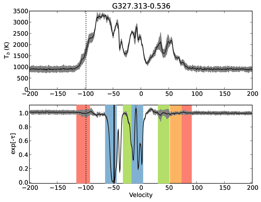
Figure 4: H I emission/absorption spectrum pairs. In each figure, the top panel shows the emission spectra. The emission is shown by the solid line (this is the average of the three “off” positions, see Section 3) and the emission envelope ($3\sigma_{T_{\rm{off}}}$) is shown in grey. Absorption, $e^{-\tau}$, is displayed in the bottom panel. The H I absorption spectrum (see Equation 3) is shown by the solid line and the grey envelope signifies $\Delta_{\textrm{abs}}$ (calculated from the emission envelope). The absorption panel also displays the fluctuation in the baseline of the absorption spectrum ($\sigma_{\rm{rms}}$) (horizontal dotted lines). The H II region name and reference are shown as well as the expected velocity ranges of Galactic structure features with the same color system as Figure 5. (A color version and the complete figure set (252 images) of this figure are available in the online journal.)

The H I emission/absorption spectra, for each included H II region, are also available in a tar file. We provide an example of this data in Table 2. For each velocity channel we provide the on source brightness temperature ($T_{\rm{on}}$); average of the three off source brightness temperatures (i.e. the emission spectrum, $T_{\rm{off}}$); the uncertainty in $T_{\rm{off}}$, caused by the differences in the three off source positions,$3\sigma_{T_{\rm{off}}}$ ; the absorption value ($e^{-\tau}$); and the $\Delta_{\textrm{abs}}$ absorption uncertainty envelope.

[1]	[2]	[3]	[4]	[5]	[6]
-10.718	5.042	3.638	0.803	1.008	0.079
-9.894	4.320	3.266	1.192	1.006	0.067
-9.069	4.932	4.621	0.758	1.002	0.078
-8.245	6.187	4.059	0.850	1.012	0.099
-7.420	6.265	6.871	1.706	0.997	0.100
-6.596	6.783	7.486	0.352	0.996	0.109
-5.771	9.314	7.669	0.612	1.009	0.152
-4.947	8.126	8.502	1.465	0.998	0.132
-4.122	9.135	8.663	0.611	1.003	0.149
-3.298	11.130	11.743	0.890	0.997	0.183
-2.473	10.098	14.215	1.997	0.977	0.165
-1.649	10.418	15.320	0.644	0.972	0.171
-0.824	12.797	16.794	1.634	0.977	0.211
0.000	15.127	20.274	2.506	0.971	0.250
0.825	18.053	23.362	2.692	0.970	0.300
1.649	15.809	28.417	1.363	0.929	0.262
2.474	6.041	33.051	3.283	0.848	0.096
3.298	-2.430	39.661	6.883	0.762	0.047
4.123	17.582	42.043	5.126	0.862	0.292
4.947	28.948	44.790	3.800	0.911	0.484
5.772	33.344	44.136	2.939	0.939	0.559
6.596	36.165	44.364	2.387	0.954	0.607
7.421	28.446	45.145	3.021	0.906	0.476
8.245	10.029	43.982	4.989	0.808	0.164
9.069	15.144	46.651	3.893	0.822	0.251
9.894	30.727	48.985	3.917	0.897	0.515
10.718	37.734	48.884	3.879	0.937	0.633

Table 2: Example of spectrum data. Columns are as follows: [1] velocity channel (km s^-1); [2] $T_{o}n$ (K); [3] average $T_{off}$ (K); [4] uncertainty in $T_{off}$, $3\sigma_{T_{\rm{off}}}$ (K); [5] absorption, $e^{-\tau}$; [6] uncertainty in absorption, $\Delta_{\textrm{abs}}$. This Table, and similar files for each H II region included in the catalog, are published in entirety in the electronic edition of the journal, a portion is shown here for guidance regarding the form and content of each file.

5 Discussion

Here we briefly discuss the global properties of the H I absorption catalog (§5.1), as well as an example of its use - investigating the $lv$ locus of the Near 3kpc Arm (see §5.2).

5.1 Longitude-Velocity Distribution

One simple application of this catalog is an investigation of the distribution of H I absorption in longitude-velocity ($lv$) space. Firstly, we construct an ‘$lv$ crayon diagram’ (Figure 5) of known Galactic structures. The Near and Far 3kpc Arm fits are provided by Dame & Thaddeus (2008) and the fourth quadrant spiral arms are taken from Vallée (2008) (who represents the Distant Arm of McClure-Griffiths et al. (2004) as the Cygnus Arm beyond the Solar Circle). The velocity width of each crayon feature is set to 20km s^-1.

For each source in the catalog (of quality factor C or better), we plot both the systemic velocity of the H II region and any associated H I absorption (Figure 5). It is clear that both the H II regions and their associated H I absorption trace the spiral arm structures, especially in the inner Galaxy. This is in keeping with Jones et al. (2013) who find that $>90\%$ of their H II region sample is associated with known spiral arm structures. H II regions are considered to be the archetypical tracers of Galactic spiral structure (Bania et al., 2010); but cold, dense gas, traced by H I absorption is also more likely to be located within the spiral arms than in the inter-arm region. Each black marker on the Figure corresponds to five consecutive velocity channels which display significant absorption. It is clear that the H I absorption is also associated with the spiral arms. This is to be expected, as dense, cold gas which is traced by H I absorption is more likely to be located within the spiral arms than in the inter-arm regions. We find H I absorption associated with all inner Galaxy spiral arms.

Figure 5 not only demonstrates the suitability of both data-sets (H II region velocities and H I absorption) as spiral arm tracers, but also their inherent velocity uncertainty distributions. Galactic streaming motions are often estimated to be on the order of $\lesssim 15$km s^-1 (Bania & Lockman, 1984; Kolpak et al., 2003), i.e. within the velocity width of the crayon diagram features. However, H I absorption associated with H II regions can extend $\sim 20$km s^-1 beyond the systemic velocity of the region (Dickey et al., 2003; Jones et al., 2013).

The association of H I absorption with a Galactic structure feature can be used to infer lower distance limits, or the location of the H II region in our Galaxy (Jones & Dickey, 2012; Jones et al., 2013).

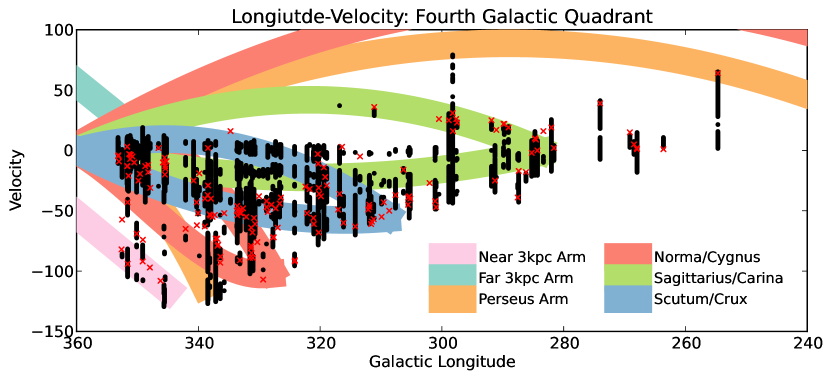
Figure 5: H II region RRL velocities (red crosses) and H I absorption (black dots) overlaid on a longitude-velocity ‘crayon diagram’. Each dot denotes the central velocity of five adjacent velocity channels ($\sim 5$km s^-1), with each channel demonstrating a statistically significant amount of H I absorption. Only H II regions with H I absorption spectra of Quality ’C’ or better are included for use in this figure. (A color version of this figure is available in the online journal.)

5.1.1 H I Absorption in the Outer Galaxy

From Figure 5 it is evident that this catalog is primarily limited to the inner Galaxy (within the Solar circle); unlike, for example, the work of Strasser et al. (2007).

Strasser et al. (2007) used the SGPS and the E/A spectrum extraction method to study H I absorption towards 111 extragalactic continuum sources - in order to investigate absorption from the outermost arms of the Milky Way. Of these 111 sources, only 17 demonstrated any signature of H I absorption at positive velocities; corresponding to a location in the outer Galaxy.

Because the Strasser et al. (2007) source sample included strictly extra-Galactic sources, the H I absorption spectra reflect lines of sight through the entire Galactic plane. Whereas spectra from this study reflect lines of sight towards the H II regions themselves, located within the Galaxy. For this reason, this work is far less likely to identify H I absorption in the outermost spiral arms in the fourth quadrant - as the number of H II regions known (with RRL velocities) is extremely limited in the most distant features.

Nevertheless, for longitudes $l<300\arcdeg$ the line of sight distance to the Solar circle is relatively small and investigations of H I absorption in the outer Galaxy become possible; although at these longitudes, there are very few known H II regions (see Figure 5). Regions with velocities $\lesssim 15$km s^-1 correspond to very short line of sight distances. At $l\approx 250\arcdeg$ the near-continuous absorption profile is associated with lines of sight through the Local Arm (catalog LOCAL ARM).

5.2 Locus of the Near 3kpc Arm

Figure 6: H I absorption associated with the Near 3kpc Arm. Left Panel: $lv$ diagram of H I absorption corresponding to the Near 3kpc Arm. Light grey dots are data from Jones et al. (2013), dark grey dots are from this work (but were not included in the linear fit analysis), black dots are also from this work (and were used in the analysis of the locus of the Arm). Right Panel: fit of data to model (Equation 8). The histogram displays the difference in velocity between Equation 8 and each channel that displays significant absorption (see Figure 5). Note only regions with $l>340\arcdeg$ are considered here.

The investigation of the $lv$ distribution of H I absorption (see Figure 5) can be further specialized to individual features. In Jones et al. (2013) the locus of the Near and Far 3kpc Arms (in $lv$ space) was investigated using H I absorption. This work presents an opportunity to extend this analysis, by including H I absorption associated with the Near 3kpc Arm at longitudes $l<350\arcdeg$. This is a complementary investigation to that first performed by Dame & Thaddeus (2008) using CO 1-0 emission.

Using H I absorption channels from the Near 3kpc Arm analysis of Jones et al. (2013) in addition to those from this work—such that the entire longitude extent 10°$>l>340$°of the Near 3kpc Arm is included—a linear fit to the $lv$ locus of the Near 3kpc Arm was performed:

$$V=-53.3+4.1l\qquad\Delta V=25.9\textrm{km s${}^{-1}$}$$ (8)

Here $\Delta V$ refers to the FWHM of a Gaussian fit to the velocity profile of the Arm model (see right hand panel of Figure 6).

With the inclusion of H I absorption from the longitude range $l<340\arcdeg$, the model for the locus of the Near 3kpc Arm (Equation 8) is extremely consistent with the fit provided by Dame & Thaddeus (2008) from CO observations; $R^{2}>0.97$ and the standard error of the mean difference is 5.4km s^-1, within the FWHM of either fit.

Figure 6 demonstrates the location of H I absorption associated with the Arm in $lv$ space, as well as an evaluation of the fit. The left hand panel, supplementary to Figure 5, is an $lv$ diagram extended to $l=10\arcdeg$ over the velocity range of the Near 3kpc Arm. Channels of significant absorption are shown, in addition to those from Jones et al. (2013). The $lv$ linear fits to the locus of the Near 3kpc Arm from Dame & Thaddeus (2008, $V=-53.1+4.6,\Delta V=19.7$ km s^-1), Jones et al. (2013, $V=-59.2+4.12,\Delta V=17.3$ km s^-1) and this work (see Equation 8) are also shown. In the right hand panel an evaluation of the fit is made. All velocity channels shown in the left-hand panel are compared to the linear Near 3kpc Arm fit (similar to the CO 1-0, Figure 2 of Dame & Thaddeus (2008)). The Near 3kpc Arm is identified as a well defined peak in H I absorption, centered around the fit to the linear model (however, the scale height of the component is exaggerated by the removal of non-Near 3kpc Arm absorption for $360\arcdeg>l>353\arcdeg$). The hump at $\Delta V=30$ (i.e. velocities consistent with a line parallel to Equation 8 $+30$km s^-1) may be the signature of the Norma Arm, which is approximately parallel to the Near 3kpc Arm in $lv$ space for longitudes $l>340\arcdeg$ (see Figure 5). The broad central peak is the result of the remaining disk rotation, both foreground and background to the Near 3kpc Arm.

Note that longitudes $l<350\arcdeg$ the Far 3kpc Arm is confused in velocity with the other inner Galaxy spiral arms - therefore investigation of the locus of the Far 3kpc Arm, extending the work of Jones et al. (2013), is not possible here.

6 Summary

The first attempt to test and interpret H I emission/absorption spectrum pairs from the SGPS (test region) was performed by Dickey et al. (2003). However, until now, no complete census of H I absorption towards Galactic continuum sources in the SGPS has been completed. This paper presents, in graphical, numerical and summary formats, the H I emission and absorption spectrum pairs from every known Galactic H II region distinctly detectable in the SGPS (255°$<l<$353°, $|b|\lesssim 1$°)—a total of 252 regions.

We have demonstrated one use of this catalog by examining the $lv$ distribution of H I absorption in the Milky Way—including a re-evaluation of the locus of the Near 3kpc Arm in $lv$ space. This catalog has the potential to be an integral data set for numerous works; perhaps even sparking the invigoration of the search for H I spiral arms of the Milky Way in absorption, rather than emission, as Lockman (2002) predicted.

References

- Bania et al. (2010) Bania, T. M., Anderson, L. D., Balser, D. S., & Rood, R. T. 2010, ApJ, 718, L106
- Bania & Lockman (1984) Bania, T. M., & Lockman, F. J. 1984, ApJS, 54, 513
- Benjamin et al. (2003) Benjamin, R. A., Churchwell, E., Babler, B. L., et al. 2003, PASP, 115, 953
- Busfield et al. (2006) Busfield, A. L., Purcell, C. R., Hoare, M. G., et al. 2006, MNRAS, 366, 1096
- Carey et al. (2009) Carey, S. J., Noriega-Crespo, A., Mizuno, D. R., et al. 2009, PASP, 121, 76
- Caswell & Haynes (1987) Caswell, J. L., & Haynes, R. F. 1987, A&A, 171, 261
- Condon et al. (1998) Condon, J. J., Cotton, W. D., Greisen, E. W., et al. 1998, AJ, 115, 1693
- Dame & Thaddeus (2008) Dame, T. M., & Thaddeus, P. 2008, ApJ, 683, L143
- Dickey et al. (2001) Dickey, J. M., McClure-Griffiths, N. M., Stanimirović, S., Gaensler, B. M., & Green, A. J. 2001, ApJ, 561, 264
- Dickey et al. (2003) Dickey, J. M., McClure-Griffiths, N. M., Gaensler, B. M., & Green, A. J. 2003, ApJ, 585, 801
- Dickey et al. (2009) Dickey, J. M., Strasser, S., Gaensler, B. M., et al. 2009, ApJ, 693, 1250
- Downes et al. (1980) Downes, D., Wilson, T. L., Bieging, J., & Wink, J. 1980, A&AS, 40, 379
- Ewen & Purcell (1951) Ewen, H. I., & Purcell, E. M. 1951, Nature, 168, 356
- Ferrière (2001) Ferrière, K. M. 2001, Reviews of Modern Physics, 73, 1031
- Foster et al. (2011) Foster, J. B., Jackson, J. M., Barnes, P. J., et al. 2011, ApJS, 197, 25
- Gibson et al. (2005) Gibson, S. J., Taylor, A. R., Higgs, L. A., Brunt, C. M., & Dewdney, P. E. 2005, ApJ, 626, 195
- Gooch (1995) Gooch, R. 1995, Astronomical Data Analysis Software and Systems IV, 77, 144
- Green (1993) Green, D. A. 1993, MNRAS, 262, 327
- Haverkorn et al. (2006) Haverkorn, M., Gaensler, B. M., McClure-Griffiths, N. M., Dickey, J. M., & Green, A. J. 2006, ApJS, 167, 230
- Hunter (2007) Hunter, J. D. 2007, Computing In Science & Engineering, 9, 90
- Jones & Dickey (2012) Jones,C., & Dickey, J. 2012, ApJ, 753, 62
- Jones et al. (2013) Jones, C., Dickey, J. M., Dawson, J. R., et al. 2013, ApJ, 774, 117
- Kavars et al. (2005) Kavars, D. W., Dickey, J. M., McClure-Griffiths, N. M., Gaensler, B. M., & Green, A. J. 2005, ApJ, 626, 887
- Kothes & Dougherty (2007) Kothes, R., & Dougherty, S. M. 2007, A&A, 468, 993
- Kolpak et al. (2003) Kolpak, M. A., Jackson, J. M., Bania, T. M., Clemens, D. P. & Dickey, J. M. 2003, ApJ, 582, 756
- Kuchar & Clark (1997) Kuchar, T. A., & Clark, F. O. 1997, ApJ, 488, 224
- Lockman (1989) Lockman, F. J. 1989, ApJS, 71, 469
- Lockman (2002) Lockman, F. J. 2002, Seeing Through the Dust: The Detection of HI and the Exploration of the ISM in Galaxies, 276, 107
- McClure-Griffiths et al. (2004) McClure-Griffiths, N. M., Dickey, J. M., Gaensler, B. M., & Green, A. J. 2004, ApJ, 607, L127
- McClure-Griffiths et al. (2005) McClure-Griffiths, N. M., Dickey, J. M., Gaensler, B. M., et al. 2005, ApJS, 158, 178
- McClure-Griffiths et al. (2012) McClure-Griffiths, N. M., Dickey, J. M., Gaensler, B. M., et al. 2012, ApJS, 199, 12
- Reifenstein et al. (1970) Reifenstein, E. C., Wilson, T. L., Burke, B. F., Mezger, P. G., & Altenhoff, W. J. 1970, A&A, 4, 357
- Roman-Duval et al. (2009) Roman-Duval, J., Jackson, J. M., Heyer, M., et al. 2009, ApJ, 699, 1153
- Stil et al. (2006) Stil, J. M., Taylor, A. R., Dickey, J. M., et al. 2006, AJ, 132, 1158
- Strasser et al. (2007) Strasser, S. T., Dickey, J. M., Taylor, A. R., et al. 2007, AJ, 134, 2252
- Taylor et al. (2003) Taylor, A. R., Gibson, S. J., Peracaula, M., et al. 2003, AJ, 125, 3145
- Urquhart et al. (2012) Urquhart, J. S., Hoare, M. G., Lumsden, S. L., et al. 2012, MNRAS, 420, 1656
- Vallée (2008) Vallée, J. P. 2008, AJ, 135, 1301
- Walsh et al. (1999) Walsh, A. J., Burton, M. G., Hyland, A. R., & Robinson, G. 1999, MNRAS, 309, 905