Lifetime of Single-Particle Excitations in a Dilute Bose-Einstein Condensate
at Zero Temperature

Abstract

We study the lifetime of single-particle excitations in a dilute homogeneous Bose-Einstein condensate at zero temperature based on a self-consistent perturbation expansion of satisfying Goldstone’s theorem and conservation laws simultaneously. It is shown that every excitation for each momentum ${\bm{p}}$ should have a finite lifetime proportional to the inverse $a^{-1}$ of the $s$-wave scattering length $a$, instead of $a^{-2}$ for the normal state, due to a new class of Feynman diagrams for the self-energy that emerges upon condensation. We calculate the lifetime as a function of $|{\bm{p}}|$ approximately.

The interaction between particles yields a finite decay rate in every single-particle excitation of many-particle systems. It is caused by collisions between particles that are describable as second- and higher-order processes of the perturbation expansion in terms of the interaction.AGD63 Hence, one may expect generally that the decay rate $\Gamma$, which is the inverse of the lifetime $\tau$ ($\hbar=1$), depends quadratically for a dilute system on the $s$-wave scattering length $a$ as $\Gamma\propto a^{2}$. We will show below, however, that this is not the case for Bose-Einstein condensates (BECs) where $\Gamma$ will be proportional to $a$.

Theoretical attempts to microscopically describe Bose-Einstein condensates have encountered fundamental difficulties due to a finite thermodynamic average $\langle\psi\rangle$ of the field operator $\psi$ itself, such as the conserving-gapless dilemmaHM65 ; Griffin96 and infrared divergences.GN64 To resolve them, a self-consistent perturbation expansion has been constructed recently in such a way as to satisfy a couple of exact statements simultaneously, i.e., conservation laws and Goldstone’s theorem.Kita09 According to it,Kita09 ; Kita11 there should be a new type of Feynman diagrams for the self-energy that are classified as “one-particle reducible” (1PR) or “improper” in the normal state,AGD63 ; LW which may modify standard results based on the Bogoliubov theoryAGD63 ; Bo substantially. For example, we have predicted in a previous paper that they will convert the Lee-Huang-Yang expressionsLHY57 for the ground-state energy per particle $E/N$ and condensate density $n_{0}$ of the dilute Bose gas intoTK13

$$\frac{E}{N}=\frac{2\pi\hbar^{2}an}{m}\left[\,1+\left(\frac{128}{15\sqrt{\pi}}+\frac{16}{5}c_{\rm ip}\right)\!\sqrt{a^{3}n}\,\right],$$ (1a)

$$\frac{n_{0}}{n}=1-\left(\frac{8}{3\sqrt{\pi}}+c_{\rm ip}\right)\!\sqrt{a^{3}n},$$ (1b)

where $m$ and $n$ are the particle mass and density, respectively, and $c_{\rm ip}$ is an extra constant of order $1$ due to those diagrams.

In the present paper, we focus on the lifetime of single-particle excitations in a dilute BEC at zero temperature. We predict that the 1PR diagrams, which are characteristic of BECs, transform the nature of the Bogoliubov mode substantially into a “bubbling” modeKita11 with a proper lifetime proportional to $a^{-1}$.

We consider a homogeneous system of identical Bose particles with mass $m$ and spin $0$ interacting via the contact potential $U\delta({\bm{r}}-{\bm{r}}^{\prime})$. The Hamiltonian is given by

$$H=\sum_{\bm{p}}(\epsilon_{p}\!-\!\mu)c^{\dagger}_{\bm{p}}c_{\bm{p}}+\frac{U}{2V}\!\sum_{{\bm{p}}{\bm{p}}^{\prime}{\bm{q}}}c^{\dagger}_{{\bm{p}}+{\bm{q}}}c^{\dagger}_{{\bm{p}}^{\prime}-{\bm{q}}}c_{{\bm{p}}^{\prime}}c_{{\bm{p}}},$$ (2)

where ${\bm{p}}$, $\epsilon_{p}\!\equiv\!p^{2}/2m$, $\mu$, and $V$ are the momentum, kinetic energy, chemical potential, and volume, and $c^{\dagger}_{\bm{p}}$ and $c_{\bm{p}}$ are the creation and annihilation operators, respectively. We set $\hbar=2m=k_{\rm B}=T_{\rm c}^{0}=1$, where $k_{\rm B}$ denotes the Boltzmann constant and $T_{\rm c}^{0}$ is the transition temperature of ideal Bose-Einstein condensation.FW71 Ultraviolet divergences inherent in the continuum model are removed here by introducing a momentum cutoff $p_{c}\gg 1$. It is standard in the low-density limit to express $U$ in terms of the s-wave scattering length $a$. They are connected in the conventional units by

$$\frac{m}{4\pi\hbar^{2}a}=\frac{1}{U}+\int\frac{d^{3}p}{(2\pi\hbar)^{3}}\frac{\theta(p_{c}-p)}{2\epsilon_{p}},$$

with $\theta(x)$ the step function, which in the present units reads

$$1/8\pi a=1/U+p_{c}/4\pi^{2}.$$ (3)

We will focus on the limit $a\rightarrow 0$ and choose $p_{c}$ so that $1\ll p_{c}\ll\pi/2a$ is satisfied; thus, $U=8\pi a$ to the leading order.

Green’s function for a homogeneous BEC can be expressed in the Nambu representation asKita09 ; Kita11

$$\hat{G}_{\vec{p}}=\begin{bmatrix}{G_{\vec{p}}}&{F_{\vec{p}}}\vspace{2mm}\\ {-\bar{F}_{\vec{p}}}&{-\bar{G}_{\vec{p}}}\end{bmatrix},$$ (4a)

where $$\vec{p}=({\bm{p}},z_{\ell}) z_{\ell}\equiv 2\pi T\ell\,i\ (\ell=0,\pm 1,\pm,2\cdots) T G_{\vec{p}}\!=\!G^{*}_{{\vec{p}}^{*}} F_{\vec{p}}\!=\!F_{-\vec{p}} \bar{G}_{\vec{p}}\!=\!G^{*}_{-\vec{p}^{*}} \hat{G}_{\vec{p}}$$ with and the temperature. The upper elements satisfy and , and a barred quantity generally denotes .Kita11 This matrix obeys the Dyson-Beliaev equationBeliaev58 ; Kita09

$$\hat{G}_{\vec{p}} =\begin{bmatrix}{z_{\ell}-\epsilon_{p}-\Sigma_{\vec{p}}+\mu}&{-\Delta_{\vec{p}}}\vspace{2mm}\\ {\bar{\Delta}_{\vec{p}}}&{z_{\ell}+\epsilon_{p}+\bar{\Sigma}_{\vec{p}}-\mu}\end{bmatrix}^{-1},$$ (4b)

which may also be regarded as defining the self-energies $\Sigma_{\vec{p}}$ and $\Delta_{\vec{p}}$ . In the self-consistent perturbation expansion, they are obtained from a functional $\Phi[\hat{G}_{\vec{p}},n_{0}]$ asKita09 ; Kita11

$$\Sigma_{\vec{p}}=-\frac{1}{T}\frac{\delta\Phi}{\delta G_{\vec{p}}},\hskip 28.45274pt\Delta_{\vec{p}}=\frac{2}{T}\frac{\delta\Phi}{\delta\bar{F}_{\vec{p}}}.$$ (5a)

In addition, $$\Phi$$ satisfies

$$\frac{1}{V}\frac{\delta\Phi}{\delta n_{0}}=\Sigma_{\vec{0}}-\Delta_{\vec{0}}$$ (5b)

in a gauge where $\Delta_{\vec{0}}$ is real. Substitution of Eq. (5a) into Eq. (4b) yields self-consistent (i.e., nonlinear) equations for $G_{\vec{p}}$ and $F_{\vec{p}}$. It also follows from Eq. (5b) that the extremal condition $\delta\Omega/\delta n_{0}\!=\!0$ for the thermodynamic potential $\Omega$ yields the Hugenholtz-Pines relationHP59

$$\mu=\Sigma_{\vec{0}}-\Delta_{\vec{0}}.$$ (6)

Equations (4)-(6) are exact statements. It has been shown that the functional $\Phi$ can be constructed as a power-series expansion in $U$ in such a way that Eq. (5), conservation laws (i.e., Noether’s theorem), and an exact relation for the interaction energy are satisfied simultaneously order by order.Kita09

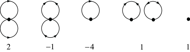
Figure 1: Feynman diagrams for $\Phi^{(1)}$. A filled circle denotes $U$, a line with an arrow (two arrows) represents $G$ (either $F$ or $\bar{F}$) in Eq. (4a) as in the theory of superconductivity,AGD63 ; FW71 and every missing line in the last three diagrams corresponds to $n_{0}$. The number below each diagram indicates its relative weight, which should be multiplied by $V/2$ to obtain the absolute weight.

Let us write down the key functional $\Phi$ perturbatively.Kita09 ; Kita11 The first-order terms are given diagrammatically in Fig. 1, which analytically reads

$$\Phi^{(1)}= \,\frac{V}{2}U\left[\sum_{\vec{p}_{1}\vec{p}_{2}}\bigl{(}2G_{\vec{p}_{1}}G_{\vec{p}_{2}}-F_{\vec{p}_{1}}\bar{F}_{\vec{p}_{2}}\bigr{)}\right.$$

$$\left.+\,n_{0}\sum_{\vec{p}}\bigl{(}-4G_{\vec{p}}+F_{\vec{p}}+\bar{F}_{\vec{p}}\bigr{)}+n_{0}^{2}\right],$$ (7)

with the summation over $\vec{p}$ defined by

$$\sum_{\vec{p}}\equiv T\sum_{\ell=-\infty}^{\infty}\frac{1}{V}\sum_{\bm{p}}.$$

It should be noted that the relative importance of each term in Eq. (7) for the dilute limit at $T\!=\!0$ increases with the power of $n_{0}$.

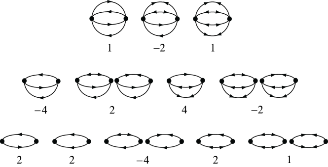
Figure 2: Feynman diagrams for $\Phi^{(2)}$. The number below each diagram indicates its relative weight, which should be multiplied by $-V/2$ to obtain the absolute weight.

Next, Fig. 2 enumerates second-order diagrams. Dominant among them in the dilute limit at $T\!=\!0$ are those in the third row proportional to $n_{0}^{2}$, i.e., those with the highest power in terms of $n_{0}$. Their contribution can be expressed concisely as

$$\Phi^{(2{\rm ip})}=-\frac{V}{2}(Un_{0})^{2}\sum_{\vec{p}}(G_{\vec{p}}+\bar{G}_{\vec{p}}-F_{\vec{p}}-\bar{F}_{\vec{p}})^{2},$$ (8a)

where $$2G_{\vec{p}}\bar{G}_{\vec{p}} G_{\vec{p}}G_{\vec{p}} \bar{G}_{\vec{p}}\bar{G}_{\vec{p}}$$, for example, corresponds to the first diagram in the third row of Fig. 2, whereas both and are associated with the second particle-particle bubble diagram to yield the same contribution.

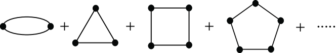
Figure 3: Feynman diagrams for $\Phi$ beyond the first order that are dominant in the dilute limit at $T\!=\!0$. Arrows are suppressed.

Extending the analysis to higher orders, one may be convinced that the leading contribution beyond the first order originates from the series of Fig. 3. These diagrams are characteristic of BECs to produce unusual 1PR self-energies upon the differentiations of Eq. (5a). However, they result naturally from the requirement that Goldstone’s theorem be satisfied order by order in $U$.Kita09 ; Kita11 They are responsible for the constant $c_{\rm ip}$ in Eq. (1),TK13 and also bring about a finite lifetime proportional to $a^{-1}$ in the single-particle excitations, as shown below. To be specific, the third-order contribution can be written asKita09 ; TK13

$$\Phi^{(3{\rm ip})}=-\frac{5V}{3}(Un_{0})^{3}\sum_{\vec{p}}(G_{\vec{p}}+\bar{G}_{\vec{p}}-F_{\vec{p}}-\bar{F}_{\vec{p}})^{3},$$ (8b)

where factor $5$ is understood as a sum of $1$ and $2^{2}$ originating from the weights of the normal particle-particle and particle-hole bubble diagrams, respectively.TK13 Both Eqs. (8a) and (8b) are given solely as a functional of

$$f_{\vec{p}}\equiv G_{\vec{p}}+\bar{G}_{\vec{p}}-F_{\vec{p}}-\bar{F}_{\vec{p}}$$ (9)

that satisfies $f_{\vec{p}}=\bar{f}_{\vec{p}}$. The statement also holds true for higher-order diagrams in the series of Fig. 3.

Thus, our approximate $\Phi$’s adopted below are all expressible as

$$\Phi[\hat{G}_{\vec{p}},n_{0}]\approx\Phi^{(1)}[\hat{G}_{\vec{p}},n_{0}]+\Phi^{({\rm ip})}[f_{\vec{p}},n_{0}],$$ (10)

where $\Phi^{(1)}$ is given by Eq. (7), and $\Phi^{({\rm ip})}[f_{\vec{p}},n_{0}]$ denotes some partial contribution from the infinite series of Fig. 3. To be specific, we consider the three approximations

$$\Phi^{({\rm ip})}\approx-V\sum_{\vec{p}}\frac{1}{2}\bigl{(}Un_{0}f_{\vec{p}}\bigr{)}^{2},$$ (11a)

$$\Phi^{({\rm ip})}\approx-V\sum_{\vec{p}}\!\left[\frac{1}{2}\bigl{(}Un_{0}f_{\vec{p}}\bigr{)}^{2}+\frac{5}{3}\bigl{(}Un_{0}f_{\vec{p}}\bigr{)}^{3}\right]\!,$$ (11b)

$$\Phi^{({\rm ip})}\approx-V\sum_{\vec{p}}\!\left[\frac{1}{2}\bigl{(}Un_{0}f_{\vec{p}}\bigr{)}^{2}+\sum_{n=3}^{\infty}\frac{1+2^{n-1}}{n}(Un_{0}f_{\vec{p}})^{n}\right]\!.$$ (11c)

The first two correspond to $\Phi^{({\rm ip})}\!\approx\!\Phi^{(2{\rm ip})}$ and $\Phi^{({\rm ip})}\!\approx\!\Phi^{(2{\rm ip})}\!+\!\Phi^{(3{\rm ip})}$ from Eq. (8), respectively, whereas the last one incorporates the contribution originating from the particle-particle and particle-hole bubbles up to the infinite order. We call them as the second-order, third-order, and fluctuation-exchange (FLEX) approximations, respectively.

The self-energies are obtained subsequently by inserting Eq. (10) into Eq. (5a), whose differentiations graphically correspond to removing a line of $G_{\vec{p}}$ and $\bar{F}_{\vec{p}}$ from every diagram for $\Phi$ in all possible ways, respectively. Note also that $G_{\vec{p}}$ and $\bar{G}_{\vec{p}}$ in Eq. (9) yield the same contribution upon the differentiation in terms of $G_{\vec{p}}$. It follows from Eq. (7) and $\Phi^{({\rm ip})}\!=\!\Phi^{({\rm ip})}[f_{\vec{p}},n_{0}]$ in Eq. (10) that the self-energies in this approximation can be expressed as

$$\Sigma_{\vec{p}}= \,\,\Sigma^{(1)}+\Delta_{\vec{p}}^{({\rm ip})},$$ (12a)

$$\Delta_{\vec{p}}= \,\,\Delta^{(1)}+\Delta_{\vec{p}}^{({\rm ip})}.$$ (12b)

Here, the first-order self-energies are given by

$$\Delta^{(1)}=U\left(n_{0}-\sum_{\vec{p}}F_{\vec{p}}\right),$$ (13a)

and $$\Sigma^{(1)}=2Un$$ with

$$n\equiv n_{0}-\sum_{\vec{p}}G_{\vec{p}}\ e^{z_{\ell}0_{+}}$$ (13b)

denoting the particle density and $0_{+}$ an infinitesimal positive constant. It is worth pointing out that $n={\zeta(3/2)}/{(4\pi)^{3/2}}$ in the present units with $\zeta(3/2)\!=\!2.612\cdots$ the Riemann zeta function.TK12 Next, $\Delta_{\vec{p}}^{({\rm ip})}$ is obtained for each approximate $\Phi^{({\rm ip})}$ in Eq. (11) as

$$\Delta^{\rm(ip)}_{\vec{p}}= \,\,2(Un_{0})^{2}f_{\vec{p}}\,,$$ (14a)

$$\Delta^{\rm(ip)}_{\vec{p}}= \,\,2(Un_{0})^{2}f_{\vec{p}}+10(Un_{0})^{3}f_{\vec{p}}^{2}\,,$$ (14b)

$$\Delta^{\rm(ip)}_{\vec{p}}= \,\,\frac{(2Un_{0})^{2}f_{\vec{p}}}{1-2Un_{0}f_{\vec{p}}}+\frac{2(Un_{0})^{2}f_{\vec{p}}}{1-Un_{0}f_{\vec{p}}}-4(Un_{0})^{2}f_{\vec{p}}\,,$$ (14c)

respectively. It follows from $f_{\vec{p}}=\bar{f}_{\vec{p}}$ in Eq. (9) that $\Delta^{\rm(ip)}_{\vec{p}}$ also satisfies $\Delta^{\rm(ip)}_{\vec{p}}=\bar{\Delta}^{\rm(ip)}_{\vec{p}}$.

Now that we have written down the self-energies explicitly, we substitute Eq. (12) into Eq. (6). We then find the Hugenholtz-Pines relation in our approximation as

$$\mu=\Sigma^{(1)}-\Delta^{(1)}.$$ (15)

Next, let us substitute Eqs. (12) and (15) into Eq. (4b) and perform the matrix inversion. We thereby obtain

$$\hat{G}_{\vec{p}}=\frac{1}{z_{\ell}^{2}-\epsilon_{p}(\epsilon_{p}+2\Delta_{\vec{p}})}\!\begin{bmatrix}z_{\ell}+\epsilon_{p}+\Delta_{\vec{p}}\!\!&\!\!\Delta_{\vec{p}}\vspace{2mm}\\ -\Delta_{\vec{p}}\!\!&\!\!z_{\ell}-\epsilon_{p}-\Delta_{\vec{p}}\end{bmatrix},$$ (16)

so that Eq. (9) is expressed concisely as

$$f_{\vec{p}}=\frac{2\epsilon_{p}}{z_{\ell}^{2}-\epsilon_{p}(\epsilon_{p}+2\Delta_{\vec{p}})}.$$ (17)

The spectral function, which has full information on the single-particle excitations, is obtained from Eq. (16) byAGD63 ; FW71

$$A_{p}(\omega)=-2\,{\rm Im}\left.G_{\vec{p}}\ \right|_{z_{\ell}\rightarrow\omega+i0_{+}}.$$ (18)

This completes our formulation.

Now, our numerical procedure to calculate the spectral function is summarized as follows. Green’s function (16) is given as a functional of $(z_{\ell},\epsilon_{p},\Delta_{\vec{p}})$ with $\Delta_{\vec{p}}\!=\!\Delta^{(1)}\!+\!\Delta_{\vec{p}}^{({\rm ip})}$, where $\Delta_{\vec{p}}^{({\rm ip})}$ is determined as a solution of the algebraic equation (14) with Eq. (17) for a given set of $(z_{\ell},\epsilon_{p},\Delta^{(1)},Un_{0})$. Besides, it follows from Eqs. (13) and (3) that

$$\Delta^{(1)}\approx Un_{0}\approx 8\pi na=\frac{\zeta(3/2)}{\sqrt{\pi}}a$$ (19)

to the leading order in $a$. Adopting this approximation, we can solve Eq. (14) with Eq. (17) as a function of $(z_{\ell}/\Delta^{(1)},\epsilon_{p}/\Delta^{(1)})$ so as to satisfy $\Delta_{\vec{p}}^{({\rm ip})}\rightarrow 0$ for $|z_{\ell}|\rightarrow\infty$. The resultant values on the imaginary axis are used subsequently to calculate Eq. (18) based on Thiele’s reciprocal difference algorithm for Padé approximants.Pade Function $A_{p}(\omega)$ thereby calculated can be checked numerically with a couple of exact relations

$$\int_{-\infty}^{\infty}\frac{d\omega}{2\pi}A_{p}(\omega)=1,$$ (20a)

$$G_{\vec{p}}=\int_{-\infty}^{\infty}\frac{d\omega}{2\pi}\frac{A_{p}(\omega)}{z_{\ell}-\omega}.$$ (20b)

We have confirmed that sum rule (20a) is satisfied beyond $99.7$%, and Green’s function on the imaginary axis are reproduced with an error of less than $0.02$%.

To start with, let us review the spectral function of the Bogoliubov theory, which is obtained by inserting Eq. (16) with $\Delta_{\vec{p}}\rightarrow\Delta^{(1)}$ into Eq. (18). It reads

$$A_{p}^{(1)}(\omega)=\pi\bigl{[}(\alpha_{p}+1)\delta\bigl{(}\omega-E^{\rm B}_{p}\bigr{)}-(\alpha_{p}-1)\delta\bigl{(}\omega+E^{\rm B}_{p}\bigr{)}\bigr{]},$$ (21)

where $E_{p}^{\rm B}\!\equiv\!\sqrt{\epsilon_{p}(\epsilon_{p}\!+\!2\Delta^{(1)})}$ is the Bogoliubov spectrum with a linear $p$ dependence for $\epsilon_{p}/\Delta^{(1)}\ll 1$, and $\alpha_{p}\equiv(\epsilon_{p}+\Delta^{(1)})/E_{p}^{\rm B}$. Thus, $A_{p}^{(1)}(\omega)$ has a couple of sharp $\delta$-function peaks at $\omega=\pm E^{\rm B}_{p}$ corresponding to well-defined quasiparticles with the infinite lifetime.

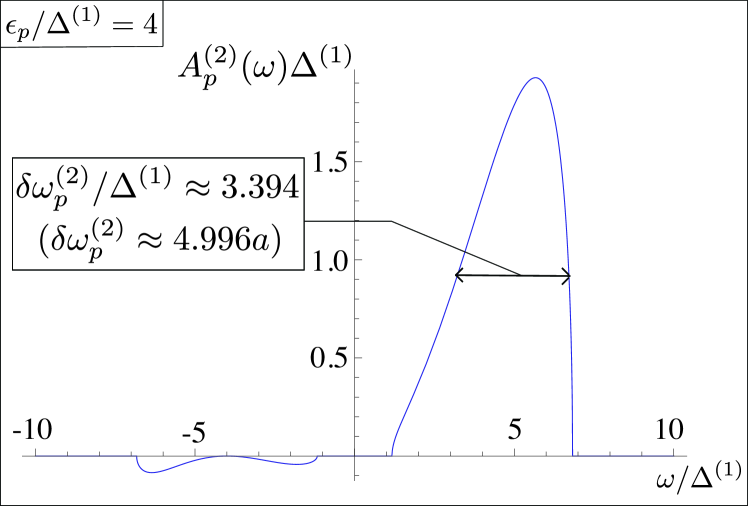
Figure 4: Plot of the spectral function $A^{(2)}_{p}(\omega)$ in the second-order approximation for $\epsilon_{p}/\Delta^{(1)}=4$. The half width $\delta\omega^{(2)}_{p}$ is proportional to $a$.

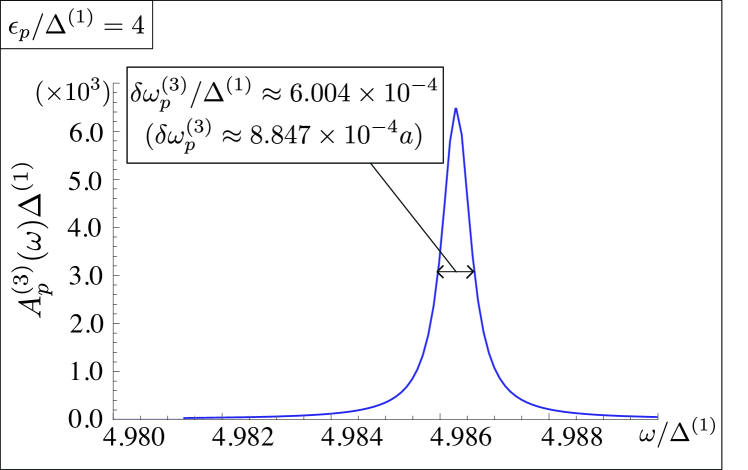
Figure 5: Plot of the spectral function $A^{(3)}_{p}(\omega)$ in the third-order approximation for $\epsilon_{p}/\Delta^{(1)}=4$.

However, the “improper” self-energy $\Delta^{({\rm ip})}_{\vec{p}}$ brings about a qualitative change in the spectral function. To see this explicitly, let us consider the second-order approximation of Eq. (14a) with Eqs. (17) and (19), which can be solved analytically as $\Delta^{({\rm ip})}_{\vec{p}}={D^{(1)}_{\vec{p}}}/{4\epsilon_{p}}-\bigl{[}\bigl{(}{D^{(1)}_{\vec{p}}}/{4\epsilon_{p}}\bigr{)}^{2}-2\bigl{(}\Delta^{(1)}\bigr{)}^{2}\bigr{]}^{1/2}$ with $D^{(1)}_{\vec{p}}\equiv(z_{\ell}-E_{p}^{\rm B})(z_{\ell}+E_{p}^{\rm B})$. Using this $\Delta^{({\rm ip})}_{\vec{p}}$ in Eq. (16) and substituting the resultant $G_{\vec{p}}$ into Eq. (18), we obtain the spectral function in the second-order approximation as

$$A^{(2)}_{p}(\omega)= \,\,\theta\bigl{(}\omega^{2}-E_{p_{-}}^{2}\bigr{)}\theta\bigl{(}E_{p_{+}}^{2}-\omega^{2}\bigr{)}[\theta(\omega)-\theta(-\omega)]$$

$$\,\,\times\frac{(\omega+\epsilon_{p})^{2}}{(4\Delta^{(1)})^{2}\epsilon_{p}^{3}}\sqrt{(E_{p_{+}}^{2}-\omega^{2})(\omega^{2}-E_{p_{-}}^{2})},$$ (22)

with $E_{p_{\pm}}\!\equiv\!\sqrt{\epsilon_{p}[\epsilon_{p}\!+\!(2\!\pm\!4\sqrt{2})\Delta^{(1)}]}$. Figure 4 exhibits $A^{(2)}_{p}(\omega)$ for $\epsilon_{p}/\Delta^{(1)}=4$. As seen clearly, the quasiparticle peaks are broadened substantially due to $\Delta^{({\rm ip})}_{\vec{p}}$. The half width $\delta\omega^{(2)}_{p}\propto\tau_{p}^{-1}$ of the main peak for $\omega>0$ is clearly of the order of $a$ and approaches $7.21a$ as $\epsilon_{p}\rightarrow\infty$. However, Eq. (22) is valid only for $\epsilon_{p}/\Delta^{(1)}\geq-2+4\sqrt{2}$; the second-order approximation fails to describe the low-momentum region adequately.

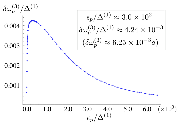
Figure 6: Half width $\delta\omega^{(3)}_{p}$ in the third-order approximation as a function of $\epsilon_{p}/\Delta^{(1)}$.

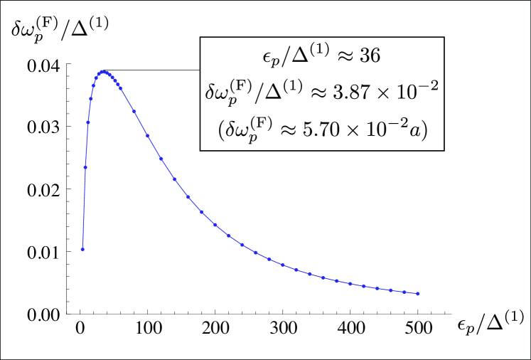
Figure 7: Half width $\delta\omega^{({\rm F})}_{p}$ in the FLEX approximation as a function of $\epsilon_{p}/\Delta^{(1)}$.

This unphysical behavior is removed in the third-order approximation of solving Eq. (14b) with Eqs. (17) and (19). Figure 5 plots the spectral function $A^{(3)}_{p}(\omega)$ in the third-order approximation for $\epsilon_{p}/\Delta^{(1)}=4$ around its peak for $\omega>0$. As seen clearly, this peak also has a finite width proportional to $a$, implying a finite lifetime $\tau_{p}\propto a^{-1}$ in the quasiparticle excitation. Figure 6 shows $\epsilon_{p}$ dependence of $\delta\omega^{(3)}_{p}\propto\tau_{p}^{-1}$. It apparently develops from zero as $\epsilon_{p}$ is increased, has the maximum around $\epsilon_{p}/\Delta^{(1)}\approx 300$, and starts to decrease thereafter towards zero. A qualitatively similar behavior is obtained by the FLEX approximation of solving Eq. (14c) with Eqs. (17) and (19), as shown in Fig. 7. However, both the magnitude of $\delta\omega^{({\rm F})}_{p}$ and its peak location are quantitatively different from $\delta\omega^{(3)}_{p}$. To resolve this point requires a better treatment of the infinite series of Fig. 3.

In summary, we have clarified that every single-particle excitation in diute BECs should have a proper lifetime even at $T\!=\!0$ that is proportional to the inverse of the $s$-wave scattering length $a$, because of the 1PR diagrams for the self-energy. The proportionality constant of the half-width $\delta\omega_{p}$ develops from zero at $p\!=\!0$, increases as momentum $p$ gets larger to have a maximum, and expected to approach $0$ eventually for $p\!\rightarrow\!\infty$.

References

(1)A. A. Abrikosov, L. P. Gorkov, and I. E. Dzyaloshinski, Methods of Quantum Field
Theory in Statistical Physics (Prentice Hall, Englewood Cliffs, N.J., 1963).
(2)P. C. Hohenberg and P. C. Martin, Ann. Phys. (N.Y.) 34, 291 (1965).
(3)A. Griffin, Phys. Rev. B 53, 9341 (1996).
(4)J. Gavoret and P. Nozières, Ann. Phys. (N.Y.) 28, 349 (1964).
(5) T. Kita, Phys. Rev. B 80, 214502 (2009).
(6) T. Kita, J. Phys. Soc. Jpn. 80, 084606 (2011).
(7) J. M. Luttinger and J. C. Ward, Phys. Rev. 118, 1417 (1960).
(8) N. N. Bogoliubov, J. Phys. (USSR) 11, 23 (1947).
(9)T. D. Lee, K. Huang, and C. N. Yang, Phys. Rev. 106, 1135 (1957).
(10) K. Tsutsui and T. Kita, J. Phys. Soc. Jpn. 82, 063001 (2013).
(11)A. L. Fetter and J. D. Walecka, Quantum Theory of Many-Particle Systems
(McGraw-Hill, New York, 1971).
(12) S. T. Beliaev, Sov. Phys. JETP 34, 323 (1958).
(13) N. M. Hugenholtz and D. Pines, Phys. Rev. 116, 489 (1959).
(14) K. Tsutsui and T. Kita, J. Phys. Soc. Jpn. 81, 114002 (2012).
(15) G. A. Baker Jr., Essentials of Padé Approximants, (Academic, New York, 1975)