The Analysis of Kademlia for random IDs

Abstract

Kademlia [7] is the de facto standard searching algorithm for P2P (peer-to-peer) networks on the Internet. In our earlier work [2], we introduced two slightly different models for Kademlia and studied how many steps it takes to search for a target node by using Kademlia’s searching algorithm. The first model, in which nodes of the network are labeled with deterministic ids, had been discussed in that paper. The second one, in which nodes are labeled with random ids, which we call the Random id Model, was only briefly mentioned. Refined results with detailed proofs for this model are given in this paper. Our analysis shows that with high probability it takes about $c\log n$ steps to locate any node, where $n$ is the total number of nodes in the network and $c$ is a constant that does not depend on $n$.

1 Introduction to Kademlia

A P2P (peer-to-peer) network [11] is a decentralized computer network which allows participating computers (nodes) to share resources. Some P2P networks have millions of live nodes. To allow searching for a particular node without introducing bottlenecks in the network, a group of algorithms called dht (Distributed Hash Table) [1] was invented in the early 2000s, including Plaxton’s algorithm [8], Pastry [10], can [9], Chord [13], Koorde [6], Tapestry [15], and Kademlia [7]. Among them, Kademlia is most widely used in today’s Internet.

In Kademlia, each node is assigned an id selected uniformly at random from $\{0,1\}^{d}$ (id space), where $d$ is usually $128$ [12] or $160$ [3]. The distance between two nodes is calculated by performing the bitwise exclusive or (xor) operation over their ids and taking the result as a binary number. (In this work distance and closeness always refer to the xor distance between ids.)

Roughly speaking, a Kademlia node keeps a table of a few other nodes (neighbors) whose distances are sufficiently diverse. So when a node searches for an id, it always has some neighbors close to its target. By inquiring these neighbors, and these neighbors’ neighbors, and so on, the node that is closest to the target id in the network will be found eventually. Other dhts work in similar ways. The differences mainly come from how distance is defined and how neighbors are chosen. For a more detailed survey of dhts, see [1].

2 The Random ID Model

This section briefly reviews the Random id Model for Kademlia defined in [2]. Let $d\geq\log_{2}n$ be the length of $n$ binary ids $X_{1},\ldots,X_{n}$ chosen uniformly at random from $\{0,1\}^{d}$ without replacement. Consider $n$ nodes indexed by $i\in\{1,\ldots,n\}$. Let $X_{i}$ be the id of node $i$.

Given two ids $x=(x_{1},\ldots,x_{d}),y=(y_{1},\ldots,y_{d})$, their xor distance is defined by

$$\delta(x,y)=\sum_{j=1}^{d}(x_{j}\oplus y_{j})\times 2^{d-j}.$$

where $\oplus$ is the xor operator

$$u\oplus v=\begin{cases}1&\text{if $u\neq v$,}\\ 0&\text{otherwise.}\end{cases}$$

Let $\ell(x,y)$ be the length of the common prefix of $x$ and $y$. The $n$ nodes can be partitioned into $d+1$ parts by their common prefix length with $x$ via

$${\cal S}(x,j)=\{i:1\leq i\leq n,~{}\ell(x,X_{i})=j\},\qquad 0\leq j\leq d.$$

For each $1\leq i\leq n$, $d$ tables (buckets) of size at most $k$ are kept, where $k$ is a fixed positive integer. Buckets are indexed by $j\in\{0,\ldots,d-1\}$. The bucket $j$ is filled with $\min\{k,|{\cal S}(X_{i},j)|\}$ indices drawn uniformly at random from ${\cal S}(X_{i},j)$ without replacement. Note that the first $j$ bits of $X_{s}$, if $s\in{\cal S}(X_{i},j)$, agree with the first $j$ bits of $X_{i}$, but the $(j+1)$-th bit is different.

Searching for $y\in\{0,1\}^{d}$ initiated at node $i$ proceeds as follows. Given that $\ell(y,X_{i})=j$, $y$ can only be in ${\cal S}(X_{i},j)$. Thus, all indices from the bucket $j$ of $i$ are retrieved, say $i_{1},\ldots,i_{k}$. From them, the one having shortest distance to $y$ is selected as $i^{*}$. (In fact, any selection algorithm would be sufficient for the results of this paper.) Note that

$$\ell(y,X_{i^{*}})=\max_{1\leq r\leq k}\ell(y,X_{i_{r}}).$$

Thus the choice of $i^{*}$ does not depend on the exact distances from $X_{i_{1}},\ldots,X_{i_{k}}$ to $y$. Therefore, instead of the xor distance, only the length of common prefix is needed in the following analysis of searching.

The search halts if $y=X_{i}$ or if the bucket is empty. In the latter case, $X_{i}$ is closest to $y$ among all nodes. Otherwise we continue from $i^{*}$. Since $\ell(y,X_{i^{*}})>\ell(y,X_{i})$, the maximal number of steps before halting is bounded by $d$. Let $T_{i}$ be the number of steps before halting in the search of $y$ when started from $i$ (searching time). Then $T_{i}=T_{i^{*}}+1$.

Treating $X_{1},\ldots,X_{n}$ as strings consisting of zeros and ones, they can be represented by a tree data structure called trie [14]. The ${\cal S}(x,j)$’s can be viewed as subtrees. Filling buckets is equivalent to choosing at most $k$ leaves from each of these subtrees. Fig. 1 gives an example of an id trie.

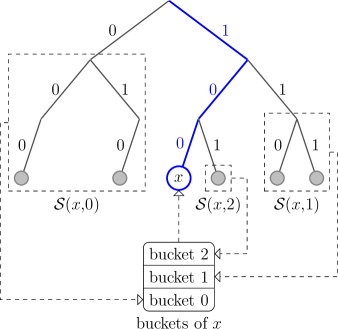
Figure 1: An example of Kademlia id trie. Given an id $x=(1,0,0)$, the trie is partitioned into subtrees ${\cal S}(x,0),{\cal S}(x,1)$ and ${\cal S}(x,2)$. Node $x$ maintains a bucket for each of these subtrees containing at most $k$ nodes from the corresponding subtree.

3 Main Results

The structure of the model is such that nothing changes if $X_{1},\dots,X_{n},y$ are replaced by their coordinate-wise xor with a given vector $z\in\{0,1\}^{d}$. This is a mere rotation of the hypercube. Thus, it can be assumed without loss of generality that $y=(1,1,\ldots,1)$, the rightmost branch in the id trie.

If $d\sim c\log_{2}n$ for some $c\geq 1$, the searching time is $O(\log n)$, which is undoubtedly a contributing factor in Kademlia’s success. If $d=\omega(n)$, then it is not a useful upper bound of searching time any more. However, in some probabilistic sense, $T_{i}$ can be much smaller than $\log_{2}n$—it can be controlled by the parameter $k$, which measures the amount of storage consumed by each node. The aim of this work is to investigate finer properties of these random variables. In particular, the following theorem is proved:

Theorem 1.

Assume that $d\geq\log_{2}n$. Let $k>0$ be a fixed integer. Let ${\,{\buildrel p\over{\rightarrow}}\,}$ denote convergence in probability. Then

$$\frac{T_{1}}{\log_{2}n}{\,{\buildrel p\over{\rightarrow}}\,}\frac{1}{\mu_{k}},\qquad\text{as }n\to\infty,$$

$$\frac{{\textbf{E}}T_{1}}{\log_{2}n}\to\frac{1}{\mu_{k}},\qquad\text{as }n\to\infty,$$

where $\mu_{k}$ is a function of $k$ only:

$$\mu_{k}=\sum_{j=1}^{\infty}1-\left(1-\frac{1}{2^{j-1}}\right)^{k}.$$

In particular, $\mu_{1}=2$.

In the rest of the paper, we first show that once the search reaches a node that shares a common prefix of length about $\log n$ with $y$, the search halts in $o(\log n)$ steps. Thus it suffices to prove Theorem 1 for the time that it takes for this event to happen. Then we show that the id trie is well balanced with high probability. Thus when $n$ is a power of $2$, we can couple the search in the original trie with a search in a trie that is a complete binary tree. It proves the theorem for this special case. After that, we give a sketch of how to deal with general $n$. At the end we briefly summarize some implications of the theorem.

4 The Tail of the Search Time

To keep the notation simple, let $m=\log_{2}n$ and and note that $m$ is not necessarily integer-valued. Also, for analytic purposes, define

$$J=\min\left\{j:\frac{n}{2^{j+1}}\leq m^{4}\right\}.$$

Since $n/2^{J}>m^{4}$ and $n/2^{J+1}\leq m^{4}$,

$$J <\log_{2}\frac{n}{m^{4}}=m-4\log_{2}m\leq m,$$ (1)

$$J \geq\log_{2}\frac{n}{m^{4}}-1=m-4\log_{2}m-1.$$ (2)

The importance of $J$ follows from the fact that once the search reaches a node $i$ with $\ell(X_{i},y)\geq J$, it takes very few steps to finish. Let ${T_{1}^{\prime}}$ be the number of search steps that depart from a node in the set ${\cal S}(y,j)$ for some $j<J$, with the very first node in the search being $1$.

Lemma 1.

Theorem 1 follows if

$$\frac{{T_{1}^{\prime}}}{\log_{2}n}{\,{\buildrel p\over{\rightarrow}}\,}\frac{1}{\mu_{k}},\qquad\text{as }n\to\infty.$$

Proof.

Let ${T_{1}^{\prime\prime}}=T_{1}-{T_{1}^{\prime}}$. ${T_{1}^{\prime\prime}}$ counts steps of the search departing from a node in $\bigcup_{j=J}^{d-1}{\cal S}(y,j)$. Thus

$${T_{1}^{\prime\prime}}\leq\sum_{j\geq J}^{d-1}{\textbf{1}_{\left[|{\cal S}(y,j)|>0\right]}}.$$

Noting that

$${\textbf{E}}|{\cal S}(y,j)|=\frac{n}{2^{j+1}},$$ (3)

by linearity of expectation,

$${\textbf{E}}{T_{1}^{\prime\prime}} \leq\sum_{j\geq J}^{d-1}{\textbf{P}}\left\{|{\cal S}(y,j)|\geq 1\right\}\leq\sum_{j\geq J}^{d-1}\min\{{\textbf{E}}|{\cal S}(y,j)|,1\}$$

$$\leq\sum_{j\geq J}^{d-1}\min\left\{\frac{n}{2^{j+1}},1\right\}\qquad(\text{by \eqref{eq:tree:expectation}})$$

$$\leq\sum_{j\geq J}^{d-1}{\textbf{1}_{\left[2^{j+1}<n\right]}}+\sum_{j\geq J}^{d-1}{\textbf{1}_{\left[2^{j+1}\geq n\right]}}\times\frac{n}{2^{j+1}}$$

$$\leq 4\log_{2}\log_{2}n+2\qquad(\text{by \eqref{eq:J:lower}}).$$

Thus, for all $\epsilon>0$ fixed,

$${\textbf{P}}\left\{{T_{1}^{\prime\prime}}\geq\epsilon\log_{2}n\right\}\leq\frac{{\textbf{E}}{T_{1}^{\prime\prime}}}{\epsilon\log_{2}n}=o(1),$$

Therefore ${T_{1}^{\prime\prime}}/\log_{2}n{\,{\buildrel p\over{\rightarrow}}\,}0$. For the expectation, note that

$$\frac{{\textbf{E}}{{T_{1}^{\prime}}}}{\log_{2}n}\to\frac{1}{\mu_{k}},\qquad\text{as }n\to\infty,$$

by the lemma’s assumption and the fact that ${T_{1}^{\prime}}/\log_{2}n\leq 1<\infty$. ∎

5 Good Tries and Bad Tries

Since the tail of search does not matter, define a new partition $S_{j}$ of all nodes by merging subtrees ${\cal S}(y,j)$ for $j\geq J$ as follows:

$${\cal S}_{j}=\begin{cases}{\cal S}(y,j)&\text{if $0\leq j<J$,}\\ \bigcup_{i=J}^{d}{\cal S}(y,i)&\text{if $j=J$}.\end{cases}$$

Let $N_{j}=|{\cal S}_{j}|$. It follows from (3) that

$${\textbf{E}}N_{j}=\begin{cases}{n}/{2^{j+1}}&\text{if $0\leq j<J$,}\\ {n}/{2^{J}}&\text{if $j=J$},\end{cases}$$ (4)

or simply ${\textbf{E}}N_{j}=n/2^{(j+1)\wedge J}$, where $a\wedge b\,{\buildrel{\rm def}\over{=}}\,\min\{a,b\}$. Note that $N_{j}$ is hypergeometric with parameters

$$\left(n,\frac{2^{d}}{2^{(j+1)\wedge J}},2^{d}-\frac{2^{d}}{2^{(j+1)\wedge J}}\right),$$

i.e., it corresponds to the selection of $n$ balls without replacement from an urn of $2^{d}$ balls of which $2^{d}/2^{(j+1)\wedge J}$ are white [5, chap. 6.3].

The analysis of ${T_{1}^{\prime}}$ can be simplified if the $N_{j}$’s are all close to their expectations. To be precise, let $\alpha=m^{-3/2}$ be the accuracy parameter. An id trie is good, if

$$\left|N_{j}-{\textbf{E}}N_{j}\right|\leq\alpha\times{\textbf{E}}N_{j},$$

for all $0\leq j\leq J$. Otherwise it is called bad.

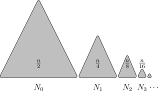
Figure 2: The approximate sizes of subtrees in a good trie.

Lemma 2.

The probability that an id trie is bad is $o(1)$.

Proof.

It follows from the union bound that

$${\textbf{P}}\left\{\bigcup_{j=0}^{J}\left[|N_{j}-{\textbf{E}}N_{j}|>\alpha\times{\textbf{E}}N_{j}\right]\right\} \leq\sum_{j=0}^{J}{\textbf{P}}\left\{\left[|N_{j}-{\textbf{E}}N_{j}|>\alpha\times{\textbf{E}}N_{j}\right]\right\}$$

$$\leq\sum_{j=0}^{J}\frac{{\textbf{Var}}(N_{j})}{(\alpha\times{\textbf{E}}N_{j})^{2}}\qquad\text{(by Chebyshev's inequality})$$

$$\leq\sum_{j=0}^{J}\frac{{\textbf{E}}N_{j}}{(\alpha\times{\textbf{E}}N_{j})^{2}}\qquad\text{($N_{j}$ is hypergeometric)}$$

$$\leq\frac{1}{\alpha^{2}}\times\sum_{j=0}^{J}\frac{2^{j+1}}{n}\qquad\text{(by \eqref{eq:N:expectation})}$$

$$\leq m^{3}\times\frac{2^{J+2}}{n}=o(1).\qquad\left(\text{since }\frac{n}{2^{J}}>m^{4}\right)$$

The fact used here is that ${\textbf{Var}}(N_{j})\leq{\textbf{Var}}(N_{j}^{\prime})$ where $N_{j}^{\prime}$ is binomial $(n,1/2^{(j+1)\wedge J})$. For the binomial, ${\textbf{Var}}(N_{j}^{\prime})\leq{\textbf{E}}N_{j}^{\prime}={\textbf{E}}N_{j}$. ∎

6 Proof when $n$ Is a Power of $2$

In this section, $n$ is assumed to be a power of $2$, i.e., $m$ is an integer. The general case is treated in the next section.

6.1 A Perfect Trie

Construct a coupled id trie consisting of $Y_{1},\ldots,Y_{n}$ as follows. If $N_{j}\geq{\textbf{E}}N_{j}$, i.e., the size of the subtree ${\cal S}_{j}$ is at least its expectation, let $Y_{i}=X_{i}$ for the ${\textbf{E}}N_{j}$ smallest indices in ${\cal S}_{j}$. After this preliminary coupling, some $Y_{i}$’s are undefined. The indices $i$ for which $Y_{i}$ are undefined go into a global pool ${\cal G}$ of size

$$\sum_{j=0}^{J}\max\{N_{j}-{\textbf{E}}N_{j},0\}.$$

For a good trie, the size of the pool is at most

$$\sum_{j=0}^{J}\alpha\times{\textbf{E}}N_{j}=\alpha\times{\textbf{E}}\sum_{j=0}^{J}N_{j}=\alpha n.$$

For a subtree ${\cal S}_{j}$ of size $N_{j}<{\textbf{E}}N_{j}$, take ${\textbf{E}}\left[N_{j}\right]-N_{j}$ indices $i$ from ${\cal G}$ and assign $Y_{i}$ a value, that is different from all other $Y_{s}$’s, and that has $\ell(Y_{i},y)\wedge J=j$. Subtrees of this new trie have fixed sizes of

$$|\{i:\ell(Y_{i},y)\wedge J=j\}|={\textbf{E}}N_{j}=\frac{n}{2^{(j+1)\wedge J}},\qquad 0\leq j\leq J.$$ (5)

A trie like this is called perfect. Indices $i$ for which $X_{i}\neq Y_{i}$, i.e., $i\in{\cal G}$, are called ghosts. Other indices are called normal.

Next, refill the buckets according to the perfect trie, but keep buckets of normal indices containing no ghosts unchanged. Observe that a search step departing at a normal index $i$ proceeds precisely the same in both tries if bucket $j$ (with $j=\ell(Y_{i},y)$) of $i$ does not contain ghosts. Assuming that the original trie is good, the probability that a bucket that corresponds to ${\cal S}_{j}$ for some $j\leq J$ contains a ghost is not more than $k\alpha$. This is because in the newly constructed prefect trie, the subtree ${\cal S}_{j}$ contains no more than $\alpha$ proportion of ghost nodes.

Let ${T_{1}^{*}}$ denote the number of search steps starting from node $1$ via node $i$ with $\ell(Y_{i},y)<J$ in the perfect trie. Then $\left[{T_{1}^{*}}\neq{T_{1}^{\prime}}\right]\subseteq B,$ where $B$ is the event that at least one node in the buckets encountered during a search is a ghost. Let $A$ be the event that the trie is good. It follows from Lemma 2 that

$${\textbf{P}}\left\{{T_{1}^{*}}\neq{T_{1}^{\prime}}\right\}\leq{\textbf{P}}\left\{B\right\}\leq{\textbf{P}}\left\{B,A\right\}+{\textbf{P}}\left\{A^{c}\right\}\leq J\times k\alpha+o(1)=o(1).$$

Therefore, Theorem 1 follows if

$$\frac{{T_{1}^{*}}}{\log_{2}n}{\,{\buildrel p\over{\rightarrow}}\,}\frac{1}{\mu_{k}},\qquad\text{as }n\to\infty.$$

6.2 Filling the Buckets with Replacement

To deal with the problem that buckets are filled by sampling without replacement, another coupling argument is needed. Let $p_{j}$ be the probability that the $k$ items sampled with replacement from a set of size $n/2^{j+1}$ are not all distinctive. Observe that by the union bound,

$$p_{j}\leq\binom{k}{2}\frac{2^{j+1}}{n}\leq\frac{k^{2}2^{j}}{n}.$$

If $\ell(Y_{i},y)=j<J$, then bucket $j$ of $i$ has $k$ elements drawn without replacement from

$${\cal S}=\{s:\ell(Y_{s},y)\geq j+1\},\quad 0\leq j<J.$$

Observe that

$$|{\cal S}|=\frac{n}{2^{j+2}}+\frac{n}{2^{j+3}}+\dots+\frac{n}{2^{J}}+\frac{n}{2^{J}}=\frac{n}{2^{j+1}}.$$

Hence, with probability $1-p_{j}$, the sampling can be seen as having been carried out with replacement.

The coupling is as follows: for all $i$ with $\ell(Y_{i},y)=j$ and all $0\leq j<J$, mark bucket $j$ of $i$ with probability $p_{j}$. When a bucket is marked, replace its entries with $k$ new entires drawn with replacement conditioned on the existence of at least one duplicate entry. In this way, all bucket entries are for a sampling with replacement. Let the search time, starting still from $1$, be denoted by ${T_{1}^{**}}$. Let $D$ be the event that during the search a marked bucket is encountered. Observe that $\left[{T_{1}^{*}}\neq{T_{1}^{**}}\right]\subseteq D.$ Therefore

$${\textbf{P}}\left\{{T_{1}^{*}}\neq{T_{1}^{**}}\right\}\leq{\textbf{P}}\left\{D\right\}\leq\sum_{j=0}^{J-1}p_{j}\leq\sum_{j=0}^{J-1}\frac{k^{2}2^{j}}{n}<\frac{k^{2}2^{J}}{n}<\frac{2k^{2}}{m^{4}}=o(1).$$

So Theorem 1 follows if

$$\frac{{T_{1}^{**}}}{\log_{2}n}{\,{\buildrel p\over{\rightarrow}}\,}\frac{1}{\mu_{k}},\qquad\text{as }n\to\infty.$$

6.3 Analyzing ${T_{1}^{**}}$ Using a Sum of I.I.D. Random Variables

Let $\Delta_{0}=\ell(Y_{1},y)$. Assume that step $t$ of the search departs from node $i$ and reaches node $i^{*}$. Let $\Delta_{t}=\ell(Y_{i^{*}},y)-\ell(Y_{i},y)$, i.e., $\Delta_{t}$ represents the progress in this step. Then

$${T_{1}^{**}}=\inf\left\{t:\sum_{s=0}^{t}\Delta_{s}\geq J\right\}.$$

Due to the recursive structure of a perfect trie, $\Delta_{1},\Delta_{2},\ldots$, although not i.i.d., should have very similar distributions. This intuition leads to the following analysis of ${T_{1}^{**}}$ by studying a sum of i.i.d. random variables.

One observation allows us to deal with truncated version of $\Delta_{t}$’s is as follows:

Lemma 3.

Let $w_{0},w_{1},\ldots$ be a sequence of real numbers with $\sum_{t\geq 0}w_{t}=\infty$. Define

$${\overline{w}}_{t}=w_{t}\wedge\left(M-\sum_{s=0}^{t-1}{\overline{w}}_{s}\right),\qquad t=0,1,2\ldots,$$

where $M$ is also a real number. Then

$$\inf\left\{t:\sum_{s=0}^{t}w_{s}\geq M\right\}=\inf\left\{t:\sum_{s=0}^{t}{\overline{w}}_{s}\geq M\right\},$$

where we define the infimum of an empty set to be $\infty$.

Proof.

Let $\tau=\inf\left\{t:\sum_{s=0}^{t}w_{s}\geq M\right\}$. If $\tau=\infty$ or $\tau=0$, the lemma is trivially true. So we assume $0<\tau<\infty$. By induction on $t$, one can show that ${\overline{w}}_{t}=w_{t}$ if $t<\tau$. Since $0<\tau$, we have ${\overline{w}}_{0}=w_{0}$, which is the induction basis. If ${\overline{w}}_{s}=w_{s}$ for all $0\leq s\leq t-1$ and $t<\tau$, then

$${\overline{w}}_{t}=w_{t}\wedge\left(M-\sum_{s=0}^{t-1}{\overline{w}}_{s}\right)=w_{t}\wedge\left(M-\sum_{s=0}^{t-1}w_{s}\right)=w_{t}.$$

Therefore $\sum_{s=0}^{t}w_{s}<M$ if and only if $\sum_{s=0}^{t}{\overline{w}}_{s}<M$. ∎

Let ${\overline{\Delta}}_{t}=\Delta_{t}\wedge\left(J-\sum_{s=0}^{t-1}{\overline{\Delta}}_{s}\right)$. It follows from the previous lemma that

$${T_{1}^{**}}=\inf\left\{t:\sum_{s=0}^{t}{\overline{\Delta}}_{s}\geq J\right\},$$

which is quite convenient as the distribution of ${\overline{\Delta}}_{t}$ is easy to compute.

Assume again that step $t$ of the search departs from node $i$ with $\ell(Y_{i},y)=j<J$. Consider one item, say $z$, in bucket $j$ of $i$. Recall that $z$ is selected uniformly at random from all indices $r$ with $\ell(r,y)\geq j+1$. Thus it follows from the structure of a perfect trie, which is given by (5), that

$${\textbf{P}}\left\{\ell(Y_{z},y)=s\right\}=\frac{\frac{n}{2^{s+1}}}{\frac{n}{2^{j+2}}+\frac{n}{2^{j+3}}+\dots+\frac{n}{2^{J}}+\frac{n}{2^{J}}}=\frac{1}{2^{s-j}},\qquad j+1\leq s<J,$$

$${\textbf{P}}\left\{\ell(Y_{z},y)\geq J\right\}=\frac{\frac{n}{2^{J}}}{\frac{n}{2^{j+2}}+\frac{n}{2^{j+3}}+\dots+\frac{n}{2^{J}}+\frac{n}{2^{J}}}=\frac{1}{2^{J-j-1}}.$$

Or shifted by $-j$,

$${\textbf{P}}\left\{\ell(Y_{z},y)-j=s\right\}=\frac{1}{2^{s}},\qquad 1\leq s<J-j,$$

$${\textbf{P}}\left\{\ell(Y_{z},y)-j\geq J-j\right\}=\frac{1}{2^{J-j-1}}.$$

If truncated by $J-j$, we obtain

$${\textbf{P}}\left\{(\ell(Y_{z},y)-j)\wedge(J-j)=s\right\}\,=\frac{1}{2^{s\wedge(J-j-1)}},\qquad 1\leq s\leq J-j.$$

Note that this is exactly the distribution of a geometric $(1/2)$ truncated by $J-j$.

Recall that among all the values of $\ell(\,\cdot,\,y)$ given by items in the bucket $j$ of $i$, the one chosen as the next stop of the search gives the maximum. Thus

$$\Delta_{t}=\max_{z\in\text{bucket }j}\{\ell(Y_{z},y)-j\}.$$

Let $Z_{1},Z_{2},\ldots$ be i.i.d. geometric $(1/2)$. Let $V=\max\{Z_{1},\ldots,Z_{k}\}$. Then

$${\overline{\Delta}}_{t} =\Delta_{t}\wedge(J-j)$$

$$=\max_{z\in\text{bucket }j}\{(\ell(Y_{z},y)-j)\}\wedge(J-j)$$

$$=\max_{z\in\text{bucket }j}\{(\ell(Y_{z},y)-j)\wedge(J-j)\}$$

$$\,{\buildrel{\cal L}\over{=}}\,\max\{Z_{1}\wedge(J-j),\ldots,Z_{k}\wedge(J-j)\}$$

$$=\max\{Z_{1},\ldots,Z_{k}\}\wedge(J-j)$$

$$=V\wedge(J-j).$$

Let $V_{0}$ be a geometric $(1/2)$ minus one. Then $V_{0}\wedge d\,{\buildrel{\cal L}\over{=}}\,\Delta_{0}$. Let $V_{1},V_{2},\ldots$ be i.i.d. random variables distributed as $V$. Let ${\overline{V}}_{t}=V_{t}\wedge(J-\sum_{s=0}^{t-1}{\overline{V}}_{s})$. Using induction and the previous argument about ${\overline{\Delta}}_{t}$, one can show that

$$\sum_{s=0}^{t}{\overline{V}}_{s}\,{\buildrel{\cal L}\over{=}}\,\sum_{s=0}^{t}{\overline{\Delta}}_{s}\qquad t=0,1,\ldots.$$ (6)

For the induction basis, note that

$${\overline{\Delta}}_{0}=\Delta_{0}\wedge J\,{\buildrel{\cal L}\over{=}}\,(V_{0}\wedge d)\wedge J=V_{0}\wedge J={\overline{V}}_{0}.$$

Assume that $\sum_{s=0}^{t-1}{\overline{V}}_{s}\,{\buildrel{\cal L}\over{=}}\,\sum_{s=0}^{t-1}{\overline{\Delta}}_{s}$ for some $t>0$. Then for all $0\leq i\leq J$,

$${\textbf{P}}\left\{\sum_{s=0}^{t}{\overline{\Delta}}_{s}=i\right\} =\sum_{j=0}^{i}{\textbf{P}}\left\{{\overline{\Delta}}_{t}=i-j~{}\left|~{}\sum_{s=0}^{t-1}{\overline{\Delta}}_{s}=j\right.\right\}{\textbf{P}}\left\{\sum_{s=0}^{t-1}{\overline{\Delta}}_{s}=j\right\}$$

$$=\sum_{j=0}^{i}{\textbf{P}}\left\{V_{t}\wedge(J-j)=i-j\right\}{\textbf{P}}\left\{\sum_{s=0}^{t-1}{\overline{V}}_{s}=j\right\}$$

$$=\sum_{j=0}^{i}{\textbf{P}}\left\{\left[{\overline{V}}_{t}=i-\sum_{s=0}^{t-1}{\overline{V}}_{s}\right]\cap\left[\sum_{s=0}^{t-1}{\overline{V}}_{s}=j\right]\right\}={\textbf{P}}\left\{\sum_{s=0}^{t}{\overline{V}}_{s}=i\right\}.$$

Thus (6) is proved. It then follows from Lemma 3 and (6) that

$${T_{1}^{**}}\,{\buildrel{\cal L}\over{=}}\,\inf\left\{t:\sum_{s=0}^{t}{\overline{V}}_{s}\geq J\right\}=\inf\left\{t:\sum_{s=0}^{t}V_{s}\geq J\right\},$$

which makes ${T_{1}^{**}}$ much easier to analyze.

Since $V<s$ if and only if $Z_{1},\ldots,Z_{k}$ are all smaller than $s$,

$${\textbf{P}}\left\{V<s\right\}=\prod_{r=1}^{k}{\textbf{P}}\left\{Z_{r}<s\right\}=\left(1-\frac{1}{2^{s-1}}\right)^{k}.$$

Therefore, by definition of $\mu_{k}$,

$${\textbf{E}}V=\sum_{s=1}^{\infty}{\textbf{P}}\left\{V\geq s\right\}=\sum_{s=1}^{\infty}1-\left(1-\frac{1}{2^{s-1}}\right)^{k}=\mu_{k}.$$

Readers familiar with renewal theory [4, chap. 4.4] can immediately see that

$$\frac{{T_{1}^{**}}}{\log_{2}n}=\frac{{T_{1}^{**}}}{J}\times\frac{J}{\log_{2}n}{\,{\buildrel p\over{\rightarrow}}\,}\frac{1}{{\textbf{E}}V}=\frac{1}{\mu_{k}},$$

which completes the proof of Theorem 1 for $n$ which is power of $2$. The following Lemma gives some more details.

Lemma 4.

If $\tau=\inf\left\{t:\sum_{s=0}^{t}V_{s}\geq M\right\}$,

$$\frac{\tau}{M/{\textbf{E}}V}{\,{\buildrel p\over{\rightarrow}}\,}1,\qquad\text{as }M\to\infty.$$

Proof.

Since $V_{0}+1$ is geometric $(1/2)$,

$${\textbf{P}}\left\{V_{0}+1\leq s\right\}=1-\frac{1}{2^{s}}\geq\left(1-\frac{1}{2^{s}}\right)^{k}={\textbf{P}}\left\{V_{1}\leq s\right\}.$$

In other words, $V_{0}\preceq V_{1}$, where $\preceq$ denotes stochastical ordering. Let

$$\tau^{\prime}=\inf\left\{t:\sum_{s=1}^{t}V_{s}\geq M\right\},\qquad\tau^{\prime\prime}=\inf\left\{t:\sum_{s=0}^{t}V_{s+1}\geq M\right\}=\tau^{\prime}-1.$$

Then $\tau^{\prime\prime}\preceq\tau$ and $\tau\leq\tau^{\prime}.$ By the strong law of large numbers, both $\tau^{\prime}/M$ and $\tau^{\prime\prime}/M$ converge to $1/{\textbf{E}}V$ almost surely. Therefore $\tau/M{\,{\buildrel p\over{\rightarrow}}\,}1/{\textbf{E}}V$. ∎

7 Proof for the General Case

In this section, the proof Theorem 1 for $n$ an arbitrary integer is only sketched as most methods used here are very similar to those in the previous section.

7.1 An Almost Perfect Trie

When $n$ is not power of $2$, ${\textbf{E}}N_{j}=n/2^{(j+1)\wedge J}$ is not guaranteed to be an integer. So a perfect trie is not well defined any more. However, let us define

$$b_{j}=\begin{cases}\lceil{\textbf{E}}N_{j}\rceil=\lceil\frac{n}{2^{j+1}}\rceil&\qquad 0\leq j<J,\\ n-\sum_{s=0}^{J-1}b_{s}=n-\sum_{s=0}^{J-1}\lceil\frac{n}{2^{s+1}}\rceil&\qquad j=J.\end{cases}$$

Then the coupling argument for perfect tries used in Section 6.1 can still be applied, now replacing ${\textbf{E}}N_{j}$ by $b_{j}$.

In this way, a trie consisting of $Y_{1},\ldots,Y_{n}$ can be constructed, with its subtrees having fixed sizes of

$$|\{i:\ell(Y_{i},y)\wedge J=j\}|=b_{j}.$$ (7)

If the original trie is good, then the number of indices $i$ for which $X_{i}\neq Y_{i}$, called ghosts, is bounded by

$$\sum_{j=0}^{J-1}\alpha\times{\textbf{E}}N_{j}+(\alpha{\textbf{E}}N_{J}+J)=\alpha n+J.$$

A trie with these properties is called almost perfect.

Let ${{T}_{1}^{*}}$ denote the number of search steps starting from node $1$ via node $i$ with $\ell(Y_{i},y)<J$ in the almost perfect trie. If ${{T}_{1}^{*}}$ and ${T_{1}^{\prime}}$ are coupled the same way as they were in Section 6.1, then $\left[{{T}_{1}^{*}}\neq{T_{1}^{\prime}}\right]\subseteq B,$ where $B$ is the event that at least one node in the buckets encountered during a search is a ghost. Let $A$ be the event that the trie is good, which has probability $o(1)$ by Lemma 2. One can check that

$${\textbf{P}}\left\{{{T}_{1}^{*}}\neq{T_{1}^{\prime}}\right\}\leq{\textbf{P}}\left\{B\right\}\leq{\textbf{P}}\left\{B,A\right\}+{\textbf{P}}\left\{A^{c}\right\}\leq mk(m^{-3/2}+\frac{m}{2^{m}})+o(1)=o(1).$$

Again, Theorem 1 follows if

$$\frac{{{T}_{1}^{*}}}{\log_{2}n}{\,{\buildrel p\over{\rightarrow}}\,}\frac{1}{\mu_{k}},\qquad\text{as }n\to\infty.$$

7.2 Filling the Buckets with Replacement

The coupling argument used in Section 6.2 to deal the problem that buckets are filled by sampling without replacement can be adapted for an almost perfect trie. Let $p_{j}$ be the probability that $k$ items sampled without replacement from a set of size $b_{j+1}+\dots+b_{J}$ have conflicts. Observe that, for $n$ large enough,

$$b_{j+1}+\dots+b_{J}\geq\frac{n}{2^{j+1}}-(j+1)\geq\frac{n}{2^{j+2}}.$$

Thus it follows from the union bound that

$$p_{j}\leq\binom{k}{2}\frac{1}{b_{j+1}+\dots+b_{J}}\leq\frac{k^{2}}{2(b_{j+1}+\dots+b_{J})}\leq\frac{2^{j+1}}{n}.$$

Let the search time of sampling without replacement be ${{T}_{1}^{**}}$. Let ${{T}_{1}^{**}}$ and ${{T}_{1}^{*}}$ be coupled in the same way as they were in Section 6.2. Let $D$ be the event that during the search an unmarked bucket is encountered. Since $\left[{{T}_{1}^{*}}\neq{{T}_{1}^{**}}\right]\subseteq D,$ one can check that

$${\textbf{P}}\left\{{{T}_{1}^{*}}\neq{{T}_{1}^{**}}\right\}\leq{\textbf{P}}\left\{D\right\}\leq\sum_{j=0}^{J-1}p_{j}<\frac{4k^{2}}{m^{4}}=o(1).$$

So once again, Theorem 1 follows if

$$\frac{{{T}_{1}^{**}}}{\log_{2}n}{\,{\buildrel p\over{\rightarrow}}\,}\frac{1}{\mu_{k}},\qquad\text{as }n\to\infty.$$

7.3 Analyzing ${T_{1}^{**}}$ Using a Sum of I.I.D. Random Variables

Consider two partitions of a line segment $L$ of length $n$. From left to right, cut $L$ into $J+1$ consecutive intervals $B_{0},\ldots,B_{J}$, with $|B_{j}|=b_{j}$, where $|a|$ denotes the length of $a$. Again, from left to right, cut $L$ into infinite many consecutive intervals $B^{\prime}_{0},B^{\prime}_{1},\ldots$, with $|B_{j}^{\prime}|=1/2^{j+1}$.

Observe that for $0\leq j<J$, $B_{j}$ and $B^{\prime}_{j}$ do not completely match since $B_{j}$ is wider than $B_{j}^{\prime}$. However, since $|B_{j}|-|B_{j}^{\prime}|\leq 1$, for $0\leq j<J$, the distance between the right endpoints of $B_{j}$ and $B_{j}^{\prime}$ is at most $J$. Therefore, the total length of unmatched regions, which are are called death zones, is $O(J^{2})$.

Let ${\overline{\Delta}}_{0},{\overline{\Delta}}_{1},\ldots$ and $V_{0},V_{1},\ldots$ be the same as in Section 6.3. A coupling between them can constructed as follows: pick one point $z_{0}$ uniformly at random from the entire $L$. If $z_{0}$ falls in interval $B_{j}$, let ${\overline{\Delta}}_{0}=j$. If $z_{0}$ falls in interval $B^{\prime}_{j}$, let $V_{0}=j$. Note that ${\overline{\Delta}}_{0}\,{\buildrel{\cal L}\over{=}}\,\ell(Y_{1},y)$. Also note that since

$${\textbf{P}}\left\{V_{0}=j\right\}={\textbf{P}}\left\{z_{0}\in B^{\prime}_{j}\right\}=\frac{|B^{\prime}_{j}|}{n}=\frac{1}{2^{j+1}},\qquad j=0,1,\ldots,$$

$V_{0}$ is geometric $(1/2)$ minus one, as desired.

Assume that $\sum_{s=0}^{t-1}{\overline{\Delta}}_{s}=j$. Pick $k$ points from the line segment starting from $B_{j+1}^{\prime}$ to the right endpoint of $L$. Let $V_{t}=s$ such that the rightmost one of the $k$ points falls into $B^{\prime}_{j+s}$. Since

$${\textbf{P}}\left\{V_{t}<s\right\} ={\textbf{P}}\left\{\text{all $k$ points are in $B^{\prime}_{j+1},\ldots,B^{\prime}_{j+s-1}$}\right\}=\left(1-\frac{1}{2^{s-1}}\right)^{k},$$

$V_{t}$ is again the maximum of $k$ i.i.d. geometric $(1/2)$.

If not all the $k$ points are in the range of $B_{j+1},\ldots,B_{J}$, keep picking more points until $k$ of them are within this region. Let ${\overline{\Delta}}_{t}=s$ such that the rightmost of the these $k$ points falls into $B_{j+s}$. Chosen in this way, ${\overline{\Delta}}_{t}$ has the same distribution as how much progress one makes at step $t$ of the search. Therefore

$${{T}_{1}^{**}}\,{\buildrel{\cal L}\over{=}}\,\inf\left\{t:\sum_{s=0}^{t}{\overline{\Delta}}_{s}\geq J\right\}.$$

It follows from Lemma 4 that if

$${{T}_{1}^{***}}=\inf\left\{t:\sum_{s=0}^{t}V_{s}\geq J\right\},$$

then ${{{T}_{1}^{***}}}/{\log_{2}n}{\,{\buildrel p\over{\rightarrow}}\,}1/{\mu_{k}}$ as $n\to\infty$.

Let $E$ be the event that at some step of the previous coupling, at least one of the first $k$ chosen points falls into death zones. Note that $[{{T}_{1}^{**}}\neq{{T}_{1}^{***}}]\subseteq E$. Therefore,

$${\textbf{P}}\left\{{{T}_{1}^{**}}\neq{{T}_{1}^{***}}\right\}\leq{\textbf{P}}\left\{E\right\}\leq\sum_{j=0}^{J-1}k\frac{J^{2}}{b_{J}}\leq\frac{m^{3}k}{m^{4}-m}=o(1).$$

So the proof of Theorem 1 when $n$ is an arbitrary integer is complete.

8 Conclusions

In a Kademlia system, one often searches for a random id. Although $T_{1}$ is the searching time for a fixed id, Theorem 1 still holds if the target $y$ is chosen uniformly at random from $\{0,1\}^{d}$.

If $d\sim c\log_{2}n$ with $c>2$, there is no essential difference between sampling the $n$ ids with or without replacement from $\{0,1\}^{d}$ as the probability of a collision in sampling with replacement is $o(1)$. This is the well known birthday problem. Since in practice, a Kademlia system hands out a new id without checking its uniqueness, it is wise to have $c>2$ since then a randomly generated id clashes with any existing id with very small probability.

Recall that $\mu_{k}=\sum_{j=1}^{\infty}1-\left(1-1/{2^{j-1}}\right)^{k}$. Since the terms in the sum decrease in $j$, $\mu_{k}$ can be bounded:

$$\mu_{k} \geq\int_{0}^{\infty}1-\left(1-\frac{1}{2^{x}}\right)^{k}\mathrm{d}x=\frac{H_{k}}{\log 2},$$

$$\mu_{k} \leq\int_{0}^{\infty}1-\left(1-\frac{1}{2^{x}}\right)^{k}\mathrm{d}x+1=\frac{H_{k}}{\log 2}+1.$$

Here $\log w$ denotes the natural logarithm of $w$, and $H_{k}=\sum_{s=1}^{k}1/s$ is the $k$-th harmonic number. Since $H_{k}\sim\log k$,

$$\lim_{k\to\infty}\frac{\mu_{k}}{\log_{2}k}=\lim_{k\to\infty}\frac{H_{k}}{\log 2\times\log_{2}k}=1.$$

Thus, $T_{1}/\log_{k}n{\,{\buildrel p\over{\rightarrow}}\,}\log_{2}k/\mu_{k}=1+o_{k}(1)$. Since $T_{1}/(\frac{1}{2}\log_{2}n){\,{\buildrel p\over{\rightarrow}}\,}1$ when $k=1$, an increase in storage by a factor of $k$ results in a modest decrease in searching time by a factor of $\log(k)/(2\log 2)$.

In [2], it has been proved that if $X_{1}=x_{1},\dots,X_{n}=x_{n}$ for fixed $x_{1},\ldots,x_{n}$, then

$$\sup_{x_{1},\ldots,x_{n}}\sup_{i}\sup_{y}{\textbf{E}}{T_{i}}\leq\left(\frac{\log 2}{H_{k}}+o(1)\right)\log_{2}n.$$

Thus Theorem 1 implies that the above upper bound is not far from tight when $k$ is large. Table 1 lists the numeric values of $1/\mu_{k}$ and $\log(2)/H_{k}$ for $k=1,\ldots,10$.

Table 1: Numeric values of $1/\mu_{k}$ and $\log(2)/H_{k}$.

$k$	$1/\mu_{k}$	$\log(2)/H_{k}$
1	0.5000000000	0.6931471806
2	0.3750000000	0.4620981204
3	0.3181818182	0.3780802804
4	0.2853260870	0.3327106467
5	0.2635627530	0.3035681083
6	0.2478426396	0.2829172166
7	0.2358018447	0.2673294911
8	0.2261891923	0.2550344423
9	0.2182781689	0.2450176596
10	0.2116151616	0.2366523364

If $k=\Theta(\log n)$, then $T_{1}\sim\log n/{\log\log n}$ in probability as $n\to\infty$. The proof of Theorem 1 is for fixed $k$ only, but one can verify that only minor changes are needed to make it work for such modest increase in $k$ as a function of $n$. More specifically, to make the coupling with searching in a perfect trie work, we only need to redefine $J=\min\{j:1/2^{j+1}<m^{7}\}$ and $\alpha=m^{-3}$. And Lemma 4 needs to use a version of the weak law of large numbers [4, thm. 2.2.4] instead of the strong law of large numbers to deal with the fact that ${\textbf{E}}V$ is not a constant anymore.

If $k=n^{\Theta(1)}$, we can show that $T_{1}=\Theta(1)$ in probability. Note that here only an upper bound of $T_{1}$ is needed. Assuming that the id trie is good, it can be proved that in each search step the length of the common prefix of the current node and the target node increases by at least $c\log n$ with high probability, where $c$ is a constant depending on $k$. Thus after at most $O(1)$ steps, the current node and the target node are both in a subtree of size at most $k$. Then the search terminates after one more step.

References

- Balakrishnan et al. [2003] H. Balakrishnan, M. F. Kaashoek, D. Karger, R. Morris, and I. Stoica. Looking up data in P2P systems. Communications of the ACM, 46(2):43–48, 2003.
- Cai and Devroye [2013] X. Cai and L. Devroye. A probabilistic analysis of Kademlia networks. In Algorithms and Computation, volume 8283 of LNCS, pages 711–721. Springer, Berlin/Heidelberg, Germany, 2013.
- Crosby and Wallach [2007] S. A. Crosby and D. S. Wallach. An analysis of BitTorrent’s two Kademlia-based dhts. Rice University, Houston, TX, USA. Available online, 2007.
- Durrett [2010] R. Durrett. Probability: Theory and Examples. Cambridge Series in Statistical and Probabilistic Mathematics. Cambridge University Press, 2010.
- Johnson et al. [2005] N. Johnson, A. Kemp, and S. Kotz. Univariate Discrete Distributions. Wiley, Hoboken, NJ, USA, 2005.
- Kaashoek and Karger [2003] M. F. Kaashoek and D. R. Karger. Koorde: A simple degree-optimal distributed hash table. In Peer-to-Peer Systems II, pages 98–107. Springer, Berlin/Heidelberg, Germany, 2003.
- Maymounkov and Mazières [2002] P. Maymounkov and D. Mazières. Kademlia: A peer-to-peer information system based on the xor metric. In Peer-to-Peer Systems, volume 2429 of LNCS, pages 53–65. Springer, Berlin/Heidelberg, Germany, 2002.
- Plaxton et al. [1999] C. G. Plaxton, R. Rajaraman, and A. W. Richa. Accessing nearby copies of replicated objects in a distributed environment. Theory of Computing Systems, 32(3):241–280, 1999.
- Ratnasamy et al. [2001] S. Ratnasamy, P. Francis, M. Handley, R. Karp, and S. Shenker. A scalable content-addressable network. SIGCOMM Computer Communication Review, 31(4):161–172, 2001.
- Rowstron and Druschel [2001] A. Rowstron and P. Druschel. Pastry: Scalable, decentralized object location, and routing for large-scale peer-to-peer systems. In Middleware 2001, volume 2218 of LNCS, pages 329–350. Springer, Berlin/Heidelberg, Germany, 2001.
- Schollmeier [2001] R. Schollmeier. A definition of peer-to-peer networking for the classification of peer-to-peer architectures and applications. In Proceedings of 1st International Conference on Peer-to-Peer Computing, pages 101–102, 2001.
- Steiner et al. [2007] M. Steiner, T. En-Najjary, and E. W. Biersack. A global view of Kad. In Proceedings of the 7th ACM SIGCOMM Conference on Internet Measurement, IMC ’07, pages 117–122, New York, NY, USA, 2007. ACM.
- Stoica et al. [2001] I. Stoica, R. Morris, D. Karger, M. F. Kaashoek, and H. Balakrishnan. Chord: A scalable peer-to-peer lookup service for internet applications. SIGCOMM Computer Communication Review, 31(4):149–160, August 2001. ISSN 0146-4833.
- Szpankowski [2011] W. Szpankowski. Average Case Analysis of Algorithms on Sequences. Wiley, Hoboken, NJ, USA, 2011.
- Zhao et al. [2004] B. Y. Zhao, L. Huang, J. Stribling, S. C. Rhea, A. D. Joseph, and J. D. Kubiatowicz. Tapestry: A resilient global-scale overlay for service deployment. IEEE Journal on Selected Areas in Communications, 22:41–53, 2004.