Discontinuous Galerkin Isogeometric Analysis of Elliptic PDEs on Surfaces

1 Introduction

The Isogeometric Analysis (IGA) was introduced by Hughes et al. (2005) and has since been developed intensively, see also monograph Cottrell et al. (2009), is a very suitable framework for representing and discretizing Partial Differential Equations (PDEs) on surfaces. We refer the reader to the survey paper by Dziuk and Elliot (2013) where different finite element approaches to the numerical solution of PDEs on surfaces are discussed. Very recently, Dedner et al. (2013) have used and analyzed the Discontinuous Galerkin (DG) finite element method for solving elliptic problems on surfaces. The IGA of second-order PDEs on surfaces that avoid errors arising from the approximation of the surface, has been introduced and numerically studied by Dede and Quarteroni (2012). Brunero (2012) presented some discretization error analysis of the DG-IGA applied to plane (2d) diffusion problems that carries over to plane linear elasticity problems which have recently been studied numerically in Apostolatos et al. (2013). The efficient generation of the IGA equations, their fast solution, and the implementation of adaptive IGA schemes are currently hot research topics. The use of DG technologies will certainly facilitate the handling of the multi-patch case.

In this paper, we use the DG method to handle the IGA of diffusion problems on closed or open, multi-patch NURBS surfaces. The DG technology easily allows us to handle non-homogeneous Dirichlet boundary condition as in the Nitsche method and the multi-patch NURBS spaces which can be discontinuous across the patch boundaries. We also derive discretization error estimates in the DG- and $L_{2}$-norms. Finally, we present some numerical results confirming our theoretical estimates.

2 Surface Diffusion Model Problem

Let us assume that the physical (computational) domain $\Omega$, where we are going to solve our diffusion problem, is a sufficiently smooth, two-dimensional generic (Riemannian) manifold (surface) defined in the physical space $\mathbb{R}^{3}$ by means of a smooth multi-patch NURBS mapping that is defined as follows. Let $\mathcal{T}_{H}=\{\Omega^{(i)}\}_{i=1}^{N}$ be a partition of our physical computational domain $\Omega$ into non-overlapping patches (subdomains) $\Omega^{(i)}$ such that $\overline{\Omega}=\bigcup_{i=1}^{N}\overline{\Omega}^{(i)}$ and $\Omega^{(i)}\cap\Omega^{(j)}=\emptyset$ for $i\neq j$, and let each patch $\Omega^{(i)}$ be the image of the parameter domain $\widehat{\Omega}=(0,1)^{2}\subset\mathbb{R}^{2}$ by some NURBS mapping $G^{(i)}:\widehat{\Omega}\rightarrow\Omega^{(i)}\subset\mathbb{R}^{3},\mathbf{\xi}=(\mathbf{\xi}_{1},\mathbf{\xi}_{2})\mapsto\mathbf{x}=(\mathbf{x}_{1},\mathbf{x}_{2},\mathbf{x}_{3})=G^{(i)}(\mathbf{\xi})$, which can be represented in the form

$$G^{(i)}(\xi_{1},\xi_{2})=\sum_{k_{1}=1}^{n_{1}}\sum_{k_{2}=1}^{n_{2}}\mathbf{P}^{(i)}_{(k_{1},k_{2})}\widehat{R}^{(i)}_{(k_{1},k_{2})}(\xi_{1},\xi_{2})$$ (1)

where $\{\widehat{R}^{(i)}_{(k_{1},k_{2})}\}$ are the bivariate NURBS basis functions, and $\{\mathbf{P}^{(i)}_{(k_{1},k_{2})}\}$ are the control points, see Cottrell et al. (2009) for a detailed description.

Let us now consider a diffusion problem on the surface $\Omega$ the weak formulation of which can be written as follows: find $u\in V_{g}$ such that

$$a(u,v)=\langle F,v\rangle\quad\forall v\in V_{0},$$ (2)

with the bilinear and linear forms are given by the relations

$$a(u,v)=\int_{\Omega}\alpha\,\nabla_{\Omega}u\cdot\nabla_{\Omega}v\,d\Omega\quad\mbox{and}\quad\langle F,v\rangle=\int_{\Omega}fv\,d\Omega+\int_{\Gamma_{N}}g_{N}v\,d\Gamma,$$

respectively, where $\nabla_{\Omega}$ denotes the so-called tangential or surface gradient, see e.g. Definition 2.3 in Dziuk and Elliot (2013) for its precise description. The hyperplane $V_{g}$ and the test space $V_{0}$ are given by $V_{g}=\{v\in V=H^{1}(\Omega):v=g_{D}\;\mbox{on}\;\Gamma_{D}\}$ and $V_{0}=\{v\in V:v=0\;\mbox{on}\;\Gamma_{D}\}$ for the case of an open surface $\Omega$ with the boundary $\Gamma=\overline{\Gamma}_{D}\cup\overline{\Gamma}_{N}$ such that $\mbox{meas}_{1}(\Gamma_{D})>0$, whereas $V_{g}=V_{0}=\{v\in V:\int_{\Omega}v\,d\Omega=0\}$ in the case of a pure Neumann problem ($\Gamma_{N}=\Gamma$) as well as in the case of closed surfaces unless there is a reaction term. In case of closed surfaces there is of course no integral over $\Gamma_{N}$ in the linear functional on the right-hand side of (2). In the remainder of the paper, we will mainly discuss the case of mixed boundary value problems on an open surface under appropriate assumptions (e.g., $\mbox{meas}_{1}(\Gamma_{D})>0$, $\alpha$ - uniformly positive and bounded, $f\in L_{2}(\Omega)$, $g_{D}\in H^{\frac{1}{2}}(\Gamma_{D})$ and $g_{N}\in L_{2}(\Gamma_{N})$ ) ensuring existence and uniqueness of the solution of (2). For simplicity, we assume that the diffusion coefficient $\alpha$ is patch-wise constant, i.e. $\alpha=\alpha_{i}$ on $\Omega^{(i)}$ for $i=1,2,\ldots,N$. The other cases including the reaction-diffusion case can be treated in the same way and yield the same results like presented below.

3 DG-IGA Schemes and their Properties

The DG-IGA variational identity

$$a_{DG}(u,v)=\langle F_{DG},v\rangle\quad\forall v\in\mathcal{V}=H^{1+s}(\mathcal{T}_{H}),$$ (3)

which corresponds to (2), can be derived in the same way as their FE counterpart, where $H^{1+s}(\mathcal{T}_{H})=\{v\in L_{2}(\Omega):v|_{\Omega^{(i)}}\in H^{1+s}(\Omega^{(i)}),\;\forall\,i=1,\ldots,N\}$ with some $s>1/2$. The DG bilinear and linear forms in the Symmetric Interior Penalty Galerkin (SIPG) version, that is considered throughout this paper for definiteness, are defined by the relationships

$$a_{DG}(u,v) = \sum_{i=1}^{N}\int_{\Omega^{(i)}}\alpha_{i}\nabla_{\Omega}u\cdot\nabla_{\Omega}v\,d\Omega$$ (4)

$$-\sum_{\gamma\in\mathcal{E}_{I}\cup\mathcal{E}_{D}}\int_{\gamma}\left(\{\alpha\nabla_{\Omega}u\cdot\mathbf{n}\}[v]+\{\alpha\nabla_{\Omega}v\cdot\mathbf{n}\}[u]\right)\,d\Gamma$$

$$+\sum_{\gamma\in\mathcal{E}_{I}\cup\mathcal{E}_{D}}\frac{\delta}{h_{\gamma}}\int_{\gamma}\alpha_{\gamma}[u][v]\,d\Gamma$$

and

$$\langle F_{DG},v\rangle = \int_{\Omega}fvd\,\Omega+\sum_{\gamma\in\mathcal{E}_{N}}\int_{\gamma}g_{N}v\,d\Gamma$$ (5)

$$+\sum_{\gamma\in\mathcal{E}_{D}}\int_{\gamma}\alpha_{\gamma}\left(-\nabla_{\Omega}v\cdot\mathbf{n}+\frac{\delta}{h_{\gamma}}v\right)g_{D}\,d\Gamma,$$

respectively, where the usual DG notations for the averages $\{\cdot\}$ and jumps $[\cdot]$ are used, see, e.g., Rivière (2008). The sets $\mathcal{E}_{I}$, $\mathcal{E}_{D}$ and $\mathcal{E}_{N}$ denote the sets of edges $\gamma$ of the patches belonging to $\Gamma_{I}=\cup\,\partial\Omega^{(i)}\setminus\{\Gamma_{D}\cup\Gamma_{N}\}$, $\Gamma_{D}$ and $\Gamma_{N}$, respectively whereas $h_{\gamma}$ is the mesh-size on $\gamma$. The penalty parameter $\delta$ must be chosen such that the ellipticity of the DG bilinear on $\mathcal{V}_{h}$ can be ensured. The relationship between our model problem (2) and the DG variational identity (3) is given by the consistency theorem that can easily be verified.

Theorem 3.1

If the solution $u$ of the variational problem (2) belongs to $V_{g}\cap H^{1+s}(\mathcal{T}_{H})$ with some $s>1/2$, then $u$ satisfies the DG variational identity (3). Conversely, if $u\in H^{1+s}(\mathcal{T}_{H})$ satisfies (3), then $u$ is the solution of our original variational problem (2).

Now we consider the finite-dimensional Multi-Patch NURBS subspace

$$\mathcal{V}_{h}=\{v\in L_{2}(\Omega):\;v|_{\Omega^{(i)}}\in V^{i}_{h}(\Omega^{(i)}),\;i=1,\ldots,N\}$$

of our DG space $\mathcal{V}$, where $V^{i}_{h}(\Omega^{(i)})=\text{span}\{R_{\textbf{k}}^{(i)}\}$ denotes the space of NURBS functions on each single-patch $\Omega^{(i)},\;i=1,\ldots,N$, and the NURBS basis functions $R_{\textbf{k}}^{(i)}=\widehat{R}^{(i)}_{\textbf{k}}\circ G^{(i)^{-1}}$ are given by the push-forward of the NURBS functions $\widehat{R}^{(i)}_{\textbf{k}}$ to their corresponding physical sub-domains $\Omega^{(i)}$ on the surface $\Omega$. Finally, the DG scheme for our model problem (2) reads as follows: find $u_{h}\in\mathcal{V}_{h}$ such that

$$a_{DG}(u_{h},v_{h})=\langle F_{DG},v_{h}\rangle,\quad\forall v_{h}\in\mathcal{V}_{h}.$$ (6)

For simplicity of our analysis, we assume matching meshes in the IGA sense, where the discretization parameter $h_{i}$ characterizes the mesh-size in the patch $\Omega^{(i)}$ whereas $p$ always denotes the underlying polynomial degree of the NURBS. Using special trace and inverse inequalities in the NURBS spaces $\mathcal{V}_{h}$ and Young’s inequality, for sufficiently large DG penalty parameter $\delta$, we can easily establish $\mathcal{V}_{h}$ coercivity and boundedness of the DG bilinear form with respect to the DG energy norm

$$\|v\|^{2}_{DG}=\sum_{i=1}^{N}\alpha_{i}\|\nabla_{\Omega}v_{i}\|_{L^{2}(\Omega^{i})}^{2}+\sum_{\gamma\in\mathcal{E}_{I}\cup\mathcal{E}_{D}}\alpha_{\gamma}\frac{\delta}{h_{\gamma}}\|[v]\|_{L^{2}(\gamma)}^{2},$$ (7)

yielding existence and uniqueness of the DG solution $u_{h}\in\mathcal{V}_{h}$ of (6) that can be determined by the solution of a linear system of algebraic equations.

4 Discretization Error Estimates

Theorem 4.1

Let $u\in V_{g}\cap H^{1+s}(\mathcal{T}_{H})$ with some $s>1/2$ be the solution of (2), $u_{h}\in\mathcal{V}_{h}$ be the solution of (6), and the penalty parameter $\delta$ be chosen large enough . Then there exists a positive constant $c$ that is independent of $u$, the discretization parameters and the jumps in the diffusion coefficients such that the DG-norm error estimate

$$\|u-u_{h}\|_{DG}^{2}\leq c\left(\sum_{i=1}^{N}\alpha_{i}h_{i}^{2t}\|u\|^{2}_{H^{1+t}(\Omega^{(i)})}\right)^{1/2},$$ (8)

holds with $t:=\min\{s,p\}$.

Proof

Let us give a sketch of the proof. By the triangle inequality, we have

$$\|u-u_{h}\|_{DG}\leq\|u-\Pi_{h}u\|_{DG}+\|\Pi_{h}u-u_{h}\|_{DG}$$ (9)

with some quasi-interpolation operator $\Pi_{h}:\mathcal{V}\mapsto\mathcal{V}_{h}$ such that the first term can be estimated with optimal order, i.e. by the term on the right-hand side of (8) with some other constant $c$. This is possible due to the approximation results known for NURBS, see, e.g., Bazilevs et al. (2006) and Cottrell et al. (2009). Now it remains to estimate the second term in the same way. Using the Galerkin orthogonality $a_{DG}(u-u_{h},v_{h})=0$ for all $v_{h}\in\mathcal{V}_{h}$, the $\mathcal{V}_{h}$ coercitivity of the bilinear form $a_{DG}(\cdot,\cdot)$, the scaled trace inequality

$$\|v\|_{L^{2}(e)}\leq Ch^{-1/2}_{E}\left(\|v\|_{L^{2}(E)}+h^{1/2+\epsilon}_{E}|v|_{H^{1/2+\epsilon}(E)}\right),$$ (10)

that holds for all $v\in H^{1/2+\epsilon}(E)$, for all IGA mesh elements $E$, for all edges $e\subset\partial E$, and for $\epsilon>0$, where $h_{E}$ denotes the mesh-size of $E$ or the length of $e$, Young’s inequality, and again the approximation properties of the quasi-interpolation operator $\Pi_{h}$, we can estimate the second term by the same term $c\left(\sum_{i=1}^{N}\alpha_{i}h_{i}^{2t}\|u\|^{2}_{H^{1+t}(\Omega^{(i)})}\right)^{1/2}$ with some (other) constant $c$. This completes the proof of the theorem.

Using duality arguments, we can also derive $L_{2}$-norm error estimates that depend on the elliptic regularity. Under the assumption of full elliptic regularity, we get $\|u-u_{h}\|_{L_{2}(\Omega)}\leq c\,h^{p+1}\|u\|_{H^{p+1}(\Omega)}$ that is nicely confirmed by our numerical experiments presented in the next section for $p=1,2,3,4$.

5 Numerical Results

The DG IGA method presented in this paper as well as its continuous Galerkin counterpart have been implemented in the object oriented C++ IGA library ”Geometry + Simulation Modules” (G+SMO) . We present some first numerical results for testing the numerical behavior of the discretization error with respect to the mesh parameter $h$ and the polynomial degree $p$ Concerning the choice of the penalty parameter, we used $\delta=2(p+2)(p+1).$

As a first example, we consider a non-homogeneous Dirichlet problem for the Poisson equation in the 2d computational domain $\Omega\subset\mathbb{R}^{2}$ called Yeti’s footprint, see also Kleiss et al. (2012), where the right-hand side $f$ and the Dirichlet data $g_{D}$ are chosen such that $u(x_{1},x_{2})=\sin(\pi x_{1})\sin(\pi x_{2})$ is the solution of the boundary value problem. The computational domain (left) and the solution (right) can be seen in Fig. 1. The Yeti footprint consists of 21 patches with varying open knot vectors $\Xi$ describing the NURBS discretization in a short and precise way, see, e.g., Cottrell et al. (2009) for a detailed definition. The knot vector for patches 1 to 16 and 21 is given as $\Xi=(0,\ldots,0,0.5,1,\ldots,1)$ in both directions whereas the knot vectors for the patches 17 to 20 are given as $\Xi_{1}=(0,\ldots,0,0.5,1,\ldots,1)$ and $\Xi_{2}=(0,\ldots,0,0.25,0.5,0.75,1,\ldots,1).$

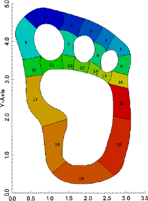
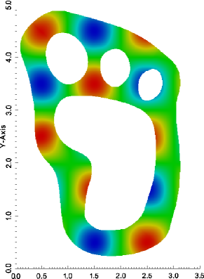
Figure 1: Yeti foot: geometry (left) and DG-IGA solution (right)

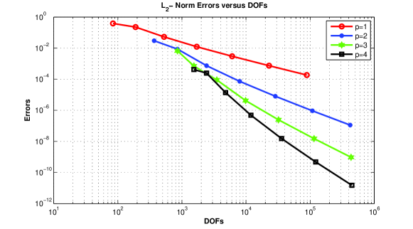
Figure 2: Yeti foot: $L_{2}-$ Norm Errors with polynomial degree $p$

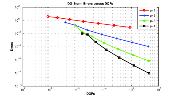
Figure 3: Yeti foot: DG Norm Errors with polynomial degree $p$

In Fig. 2 and 3, the errors in the $L_{2}$-norm and in the DG energy norm (7) are plotted against the degree of freedom (DOFs) with polynomial degrees from 1 to 4. It can be observed that we have convergence rates of $\mathcal{O}(h^{p+1})$ and $\mathcal{O}(h^{p})$ respectively. This corresponds to our theory in Section 4.

In the second example, we apply the DG-IGA to the same Laplace-Beltrami problem on an open surface as described in Dede and Quarteroni (2012), section 5.1, where $\Omega$ is a quarter cylinder represented by four patches in our computations, see Fig. 4 (left). The $L_{2}-$norm errors plotted on the right side of Fig. 4 exhibit the same numerical behavior as in the plane case of the Yeti foot. The same is true for the DG-norm.

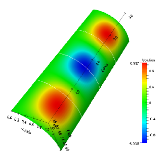
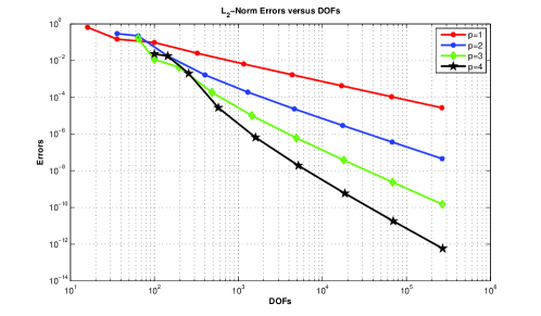
Figure 4: Quarter cylinder: geometry with the solution (left) and $L_{2}$ norm errors (right).

6 Conclusions

We have developed and analyzed a new method for the numerical approximation of diffusion problems on open and closed surfaces by combining the discontinuous Galerkin technique with isogeometric analysis. We refer to our approach as the Discontinuous Galerkin Isogeometric Analysis (DG-IGA). In our DG approach we allow discontinuities only across the boundaries of the patches, into which the computational domain is decomposed, and enforce the interface conditions in the DG framework. For simplicity of presentation, we assume that the meshes are matching across the patches, and the solution $u$ is at least patch-wise in $H^{1+s}$, i.e. $u\in H^{1+s}(\mathcal{T}_{H})$, with some $s>1/2$. The cases of non-matching meshes and low-regularity solution, that are technically more involved and that were investigated, e.g., by Dryja (2003) and Pietro and Ern (2012), will be considered in a forthcoming paper. The parallel solution of the DG-IGA equations can efficiently be performed by Domain Decomposition (DD) solvers like the IETI technique proposed by Kleiss et al. (2012), see also Apostolatos et al. (2013) for other DD solvers. The construction and analysis of efficient solution strategies is currently a hot research topic since, beside efficient generation techniques, the solvers are the efficiency bottleneck in large-scale IGA computations.

References

- Apostolatos et al. [2013] A. Apostolatos, R. Schmidt, R. Wüchner, and K.-U. Bletzinger. A Nitsche-type formulation and comparison of the most common domain decomposition methods in isogeometric analysis. Int. J. Numer. Methods Eng., 2013. URL http://dx.doi.org/10.1002/nme.4568. published online first.
- Bazilevs et al. [2006] Y. Bazilevs, L. Beirão da Veiga, J.A. Cottrell, T.J.R. Hughes, and G. Sangalli. Isogeometric analysis: Approximation, stability and error estimates for -refined meshes. Comput. Methods Appl. Mech. Engrg., 194:4135–4195, 2006.
- Brunero [2012] F. Brunero. Discontinuous Galerkin methods for isogeometric analysis. Master’s thesis, Università degli Studi di Milano, 2012.
- Cottrell et al. [2009] J.A. Cottrell, T.J.R. Hughes, and Y. Bazilevs. Isogeometric Analysis: Toward Integration of CAD and FEA. John Wiley & Sons, Chichester, 2009.
- Dede and Quarteroni [2012] L. Dede and A. Quarteroni. Isogeometric analyis for second order partial differential equations on surfaces. MATHICSE Report 36.2012, Politecnico di Milano, 2012.
- Dedner et al. [2013] A. Dedner, P. Madhavan, and B. Stinner. Analysis of the discontinuous Galerkin method for elliptic problems on surfaces. IMA J. Numer. Anal, 33(3):952–973, 2013.
- Dryja [2003] M. Dryja. On discontinuous Galerkin methods for elliptic problems with discontinuous coeffcients. Comput. Methods Appl. Math., 3:76–85, 2003.
- Dziuk and Elliot [2013] G. Dziuk and C.M. Elliot. Finite element methods for surface pdes. Acta Numerica, 22:289–396, 2013.
- Hughes et al. [2005] T.J.R. Hughes, J.A. Cottrell, and Y. Bazilevs. Isogeometric analysis: CAD, finite elements, NURBS, exact geometry and mesh refinement. Comput. Methods Appl. Mech. Engrg., 194:4135–4195, 2005.
- Kleiss et al. [2012] S. K. Kleiss, C. Pechstein, B. Jüttler, and S. Tomar. IETI – Isogeometric Tearing and Interconnecting. Comput. Methods Appl. Mech. Engrg., 247 - 248(0):201–215, 2012.
- Pietro and Ern [2012] D.A. Di Pietro and A. Ern. Mathematical Aspects of Discontinous Galerkin Methods, volume 69 of Mathématiques et Applications. Springer-Verlag, Heidelberg, Dordrecht, London, New York, 2012.
- Rivière [2008] B. Rivière. Discontinuous Galerkin Methods for Solving Elliptic and Parabolic Equations: Theory and Implementation. SIAM, Philadelphia, 2008.