On the Use of Cherenkov Telescopes for Outer Solar System Body Occultations
Abstract
Imaging Atmosphere Cherenkov Telescopes (IACT) are arrays of very large optical telescopes that are well-suited for rapid photometry of bright sources. I investigate their potential in observing stellar occultations by small objects in the outer Solar System, Transjovian Objects (TJOs). These occultations cast diffraction patterns on the Earth. Current IACT arrays are capable of detecting objects smaller than 100 metres in radius in the Kuiper Belt and 1 km radius out to 5000 AU. The future Cherenkov Telescope Array (CTA) will have even greater capabilities. Because the arrays include several telescopes, they can potentially measure the speeds of TJOs without degeneracies, and the sizes of the TJOs and background stars. I estimate the achievable precision using a Fisher matrix analysis. With CTA, the precisions of these parameter estimations will be as good as a few percent. I consider how often detectable occultations occur by members of different TJO populations, including Centaurs, Kuiper Belt Objects (KBOs), Oort cloud objects, and satellites and Trojans of Uranus and Neptune. The great sensitivity of IACT arrays means that they likely detect KBO occultations once every hours when looking near the ecliptic. IACTs can also set useful limits on many other TJO populations.
keywords:
Kuiper belt: general — Oort cloud — minor planets, asteroids, general — occultations1 Introduction
There are many minor bodies in the Solar System beyond the orbit of Jupiter, the Transjovian Objects (TJOs). There are several populations of TJOs. These include the Centaurs, a collection of objects that orbits between Jupiter and Neptune; the Kuiper Belt, a reservoir of bodies such as Pluto orbiting 30 - 50 AU from the Sun; the Scattered Disc Objects, a lower density population (among them, Eris; Brown05; Brown07) that extends out to 100 - 200 AU (e.g., Gladman08); and the Oort Cloud, a population of comets that is generally believed to mostly reside tens of thousands of AUs from the inner Solar System, but includes objects like Sedna that orbit hundreds of AU away (Brown04). The TJOs formed out of the debris left over after planet formation, and their physical properties potentially contain information about the early Solar System. Their orbits also record the effects of gravitational perturbations from the planets, and constrain models of Solar System dynamics (e.g., Morbidelli08).
Because the TJOs are in the distant reaches of the Solar System, our ability to observe and understand them is limited. Large TJOs can be directly observed with telescopes; following the early discovery of Pluto, other large TJOs were found with surveys starting in the 1990s (e.g., Jewitt93; Brown04; Brown05; Kavelaars08; Trujillo08). These big objects have been studied intensely with photometry and spectroscopy (e.g., Lazzarin03; Peixinho04; Stransberry08). Pluto itself, and possibly more distant Kuiper Belt objects, will be visited by the New Horizons probe, which will increase our understanding of TJOs (Stern08).111Triton, the largest moon of Neptune, is likely a captured Kuiper Belt object (e.g., Agnor06), and was visited by Voyager 2 in 1989. However, its structure was radically altered by its capture (e.g., McKinnon95). However, TJOs with radii of a kilometre or less are far more difficult to observe. General constraints on the amount of mass in small bodies can be found from the level of CMB anisotropies (Babich07; Ichikawa11), the brightness of the infrared background (Kenyon01), and the gamma-ray background (Moskalenko08; Moskalenko09).
The main method of searching for these small objects is through stellar occultations, when they pass in front of a background star, blocking and diffracting its light (Bailey76; Dyson92; Roques87; Roques00). At least two TJOs were detected with this method in the past few years (Schlichting09; Schlichting12). The Fresnel scale for objects in the outer Solar System is . Objects larger than essentially cast a geometrical shadow on the Earth, while smaller objects cast a diffraction pattern on the Earth as wide as , with the star’s magnitude fluctuations set by the size of the occulter.
Observing these events poses several challenges. First, the depth of the fluctuations for the smaller TJOs is typically only of order a few percent. Second, because the Earth moves with a relative speed of up to with respect to TJOs, the events last only a fraction of a second. High quality light curves must be therefore sampled with a frequency 5 – 100 Hz (cf., Nihei07, hereafter N07).
Past and present surveys for TJO occultations include TAOS, the Taiwanese American Occultation Survey, which is dedicated to detecting TJO occultations (Lehner09); additionally, surveys have been carried out on the MMT observatory (Bianco09), the Panoramic Survey Telescope and Rapid Response System 1 (PS1) telescope (Wang10), the Very Large Telescope (Doressoundiram13), and Hubble Space Telescope (Schlichting09). Additional searches for occultations of Sco X-1 in the X-ray band have been conducted, but instrumental effects proved troublesome (Chang06; Chang07; Jones08; Liu08; Chang11). Historically, a big problem with the occultation method in visible light is scintillation noise, which dominates fluctuations at short frequencies. The technique therefore requires large telescopes with high frequency sampling, and must deal with scintillation by either having a large signal-to-noise ratio (Wang10; Doressoundiram13), using multiple telescopes as a veto (Bianco10; Lehner10), or using space telescopes to eliminate it altogether (Schlichting09).
Many of these conditions are fulfilled by the Imaging Atmospheric Cherenkov Telescopes (IACTs), which are among the largest optical telescopes in the world. Cherenkov telescopes are used to detect TeV gamma-rays by imaging the flash of Cherenkov light emitted by particle showers created when the gamma ray hits the upper atmosphere (e.g., Galbraith53; Aharonian97). The flashes are faint, so the Cherenkov telescopes must be large to collect as many photons as possible (see Table 1). In addition, the Cherenkov flashes are very short, only a few nanoseconds long, so Cherenkov telescopes use photomultipliers or silicon photon detectors to sample fluxes on MHz time-scales. The optical field of view of a Cherenkov telescopes is a few degrees. Finally, Cherenkov telescopes often come in arrays, allowing them to image a particle shower in three dimensions, but this could also be useful for vetoing occultation false positives.
Cherenkov telescopes achieve this remarkable performance at a low cost by sacrificing angular resolution: the typical point spread function (PSF) of a Cherenkov telescope is a few arcminutes (Bernlohr03; Cornils03). This increases the noise of a source because of blending with more sky background. However, for the brightest sources (with ), the Poisson noise of the star is greater than the sky background noise, and confusion only becomes a problem at (Bahcall80). Therefore, the Cherenkov telescopes may be very useful for observing bright stars. Cherenkov telescopes have been used to study the Crab pulsar optical light curve (Hinton06; Lucarelli08), optical transients on millisecond and microsecond time-scales (Deil09), and for optical SETI (Eichler01; Holder05), and they are potentially good for stellar intensity interferometry (LeBohec06), detecting picosecond optical transients (Borra10) and optical polarimetry (Lacki11).
Current Cherenkov telescope arrays include the Very Energetic Radiation Imaging Telescope Array System (VERITAS)222http://veritas.sao.arizona.edu/ and the High Energy Stereoscopic System (HESS)333http://www.mpi-hd.mpg.de/hfm/HESS/ (see Table 1). VERITAS consists of four 12-meter telescopes and is located in the Northern hemisphere (Weekes02). HESS is an array of four 12-meter telescopes plus a central, fifth 28-meter telescope, located in the Southern hemisphere (Bernlohr03; Cornils03; Cornils05). The power of Cherenkov telescopes will increase much further with the next generation Cherenkov Telescope Array (CTA).444http://www.cta-observatory.org/ The array will include four large () telescopes, as well as tens of medium () and small () telescopes (Bernlohr13). The sheer number of telescopes will allow a vast number of photons to be collected, and would efficiently eliminate false positives.
The precise observations of stellar occultations that are possible with Cherenkov telescopes can be useful for studying not only the TJOs themselves but the occulted stars. The shape of the light curve depends on the size of the TJO, as well as the angular size of the star, in units of the Fresnel scale. An array of telescopes, by sampling the light curve at different positions, could measure the size of the diffraction pattern, giving the Fresnel scale, from which these parameters and the TJO distance can be calculated. Besides these parameters, the arrays can measure the position of the TJO on the sky, and the non-radial components of the TJO velocity.
| Array | Range | Baseline Range | References | ||
|---|---|---|---|---|---|
| TAOS | 4 | 0.5 | 0.79 | 7.6 – 100 | (1) |
| Megacam/MMT | 1 | 6.5 | 33 | … | (2) |
| ULTRACAM/VLT | 1 | 8.2 | 53 | … | (3) |
| VERITAS | 4 | 12.0 | 450 | 83 – 180 | (4) |
| HESS | 5 | 12.0 – 28.0 | 1100 | 85 – 170 | (5) |
| CTA (E) | 59 | 7.2 – 24.0 | 5800 | 67 – 3500 | (6) |
References – (1) Lehner09; (2) – as used in Bianco09; (3) – as used in Doressoundiram13; (4) – Weekes02, present configuration given in Perkins09; (5) – see Bernlohr03, Cornils05, and the HESS website, http://www.mpi-hd.mpg.de/hfm/HESS; (6) – configuration E given in Bernlohr13
In Lacki11, I computed the expected signal-to-noise ratios for photometric, spectroscopic, and polarimetric measurements by Cherenkov telescopes given the large sky noise. Noting that these ratios were better for bright sources, I listed several possible phenomena that might be studied optically with Cherenkov telescopes, including stellar occultations by TJOs. Now I evaluate the abilities of Cherenkov telescopes to detect and characterize these occultations. After describing how I calculate the light curves of occultation events in Section 2, I evaluate the types of events that are detectable at VERITAS, HESS, and CTA in Section 3. The ability of Cherenkov telescopes to estimate the parameters of an occultation is evaluated with Fisher matrix analysis and likelihood ratio analysis in Section 4. Finally, the frequency that these arrays should observe TJO occultations is calculated in Section 5.
2 Calculation of Light Curves and Derivatives
2.1 Observing Geometry
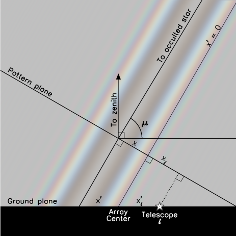
Suppose a TJO occults a star at altitude and azimuth . Each telescope is located at coordinates on the ground, which slices through the diffraction pattern at an angle. To calculate the intensity of the diffraction pattern at each telescope, we first project their positions on to the pattern plane that is normal to the line of sight to the TJO (Figure 1). With some algebra, one can show that the coordinates of the telescope on the pattern plane is
| (1) | |||||
| (2) |
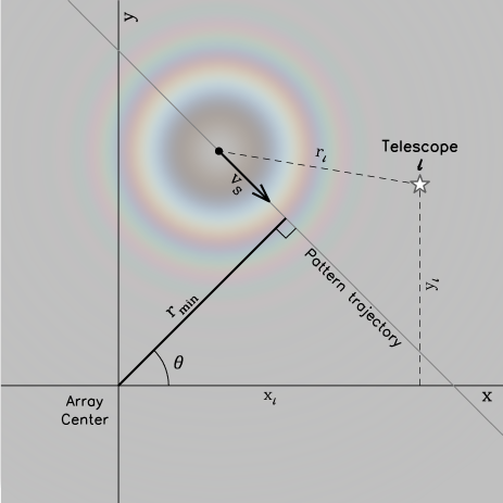
In the pattern plane, the diffraction pattern has a centre and moves at a speed . The pattern passes a minimum distance from the origin at time , when it will be at angle with respect to the x-axis (Figure 1). Thus the coordinates of the diffraction pattern in the pattern plane are
| (3) | |||||
| (4) |
where I have defined . The projected distance of the telescope from the centre of the shadow at any time is given by
| (5) | |||||
Diffraction theory gives the intensity of the diffraction pattern in terms of .
2.2 Measured Stellar Spectra
The actual diffraction pattern on Earth can be considered as the sum of diffraction patterns from each point on the background star and at each wavelength. It is this integrated diffraction pattern that photodetectors actually measure. At least two properties of the background star affect the integrated diffraction pattern: the angular size of the star and its spectrum.
I start by using the Pickles UVILIB library of stellar spectra, which covers the entire spectral range detected by the photomultiplier tubes (PMTs) used on Cherenkov telescopes for a variety of spectral types and classes (Pickles98). Pickles98 also gives the absolute bolometric magnitude, bolometric correction, and the effective temperature; from these quantities, I get the radius of the star.
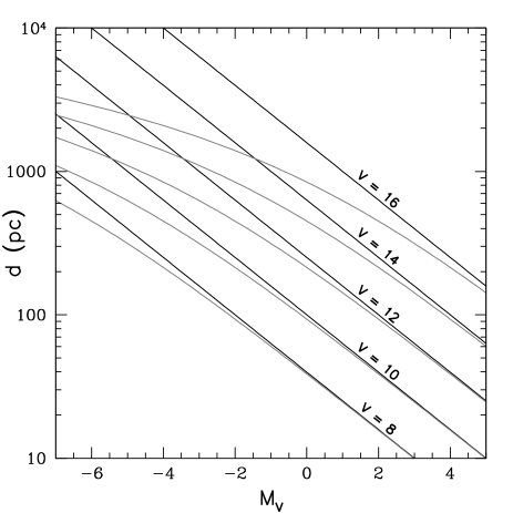
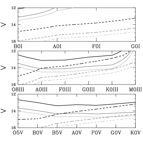
To convert radius into angular diameter and V-band absolute magnitude to V-band magnitude, I also need the distance to star at a given V-band magnitude. In practice this is complicated by the presence of dust extinction, particularly on lines of sight through the Galaxy. This effect is illustrated in Figure 2: at a given , dust extinction implies that stars are nearer than expected. The effects of dust extinction cannot be ignored for intrinsically bright stars: these are typically viewed from farther away through a larger column of dust. To account for dust extinction, I use the extinction curve of Draine03. I assume that the mean density of the Galaxy is when calculating the gas column, where is some scale factor. Then,
| (6) |
and the distance to the star is calculated by solving the equation
| (7) |
Since dust-extincted stars at a given apparent are closer to Earth than unextincted stars, they appear bigger on the sky. This blurs out the diffraction pattern more. I list my calculated stellar sizes for in Table 2.
| Type | ||||||||||||
|---|---|---|---|---|---|---|---|---|---|---|---|---|
| (pc) | () | (AU) | (pc) | () | (AU) | (pc) | () | (AU) | (pc) | () | (AU) | |
| O5V | 1500 | 36 | 60 | 2200 | 24 | 130 | 3000 | 18 | 250 | 3800 | 14 | 420 |
| B0V | 970 | 27 | 110 | 1600 | 17 | 270 | 2300 | 12 | 590 | 3100 | 8.5 | 1100 |
| B5V | 310 | 35 | 64 | 630 | 17 | 250 | 1100 | 9.9 | 790 | 1700 | 6.3 | 1900 |
| A0V | 250 | 52 | 29 | 520 | 25 | 120 | 940 | 14 | 400 | 1500 | 8.6 | 1000 |
| F0V | 94 | 71 | 16 | 220 | 31 | 82 | 450 | 15 | 360 | 850 | 7.8 | 1300 |
| G0V | 54 | 110 | 6.6 | 130 | 46 | 37 | 290 | 20 | 180 | 580 | 10 | 750 |
| K0V | 30 | 140 | 38 | 73 | 59 | 23 | 170 | 25 | 120 | 370 | 12 | 580 |
| O8III | 1600 | 48 | 34 | 2300 | 33 | 73 | 3100 | 24 | 130 | 4000 | 19 | 220 |
| A0III | 330 | 55 | 26 | 650 | 28 | 100 | 1100 | 16 | 300 | 1800 | 10 | 740 |
| F0III | 210 | 69 | 16 | 440 | 33 | 73 | 830 | 17 | 260 | 1400 | 10 | 710 |
| G0III | 130 | 130 | 4.7 | 300 | 58 | 23 | 600 | 29 | 92 | 1100 | 16 | 290 |
| K0III | 79 | 180 | 2.5 | 180 | 77 | 13 | 390 | 36 | 61 | 750 | 19 | 220 |
| M0III | 400 | 570 | 0.24 | 760 | 300 | 0.88 | 1300 | 180 | 2.5 | 2000 | 120 | 5.8 |
| B0I | 2100 | 58 | 23 | 2900 | 44 | 42 | 3800 | 32 | 75 | 4700 | 26 | 120 |
| A0I | 1900 | 170 | 2.8 | 2700 | 110 | 5.5 | 3500 | 90 | 9.6 | 4500 | 71 | 15 |
| F0I | 2000 | 250 | 1.3 | 2800 | 180 | 2.5 | 3600 | 130 | 4.3 | 4500 | 110 | 6.8 |
| G0I | 1900 | 490 | 0.33 | 2700 | 350 | 0.64 | 3600 | 260 | 1.1 | 4500 | 210 | 1.7 |
| K2I | 1800 | 880 | 0.10 | 2600 | 620 | 0.20 | 3400 | 470 | 0.36 | 4300 | 370 | 0.57 |
| M2I | 2000 | 2700 | 0.011 | 2800 | 1900 | 0.021 | 3600 | 1500 | 0.037 | 4600 | 1200 | 0.058 |
is the distance at which . Beyond this distance, the size of the stellar disc reduces the variability from the occultation. The fiducial star is marked in bold.
Not all of the photons that reach Earth are measured by the detector. Some are absorbed by the optics, and the detector responds to the remaining photons with some efficiency that varies with wavelength. I assume the detection efficiency of a PMT is
| (8) |
and 0 at other wavelengths (based on the PMT sensitivity curve given in Preu02) where is the throughput of the optical system of the IACTs.
I also consider an “ideal” detector efficiency between and .
The measured spectrum of the star is then
| (9) |
where is the optical depth of the dust as calculated using the Draine03 extinction curve.
2.3 The Diffraction Pattern
The ratio of a monochromatic point source’s flux as the occulter passes to its unobscured flux is given by
| (10) |
when , and
| (11) |
when (Roques87). Here, is the -th Lommel function, and .
Suppose the star has an angular radius , with a flux . The photon flux ratio observed by the telescope is (Roques00)
| (12) |
In this equation, , , and is the photon number flux spectrum of the star (since the detector counts photons, not energy). is normalized by the typical photon flux from the star:
| (13) |
I assume that the stellar spectrum is constant over the star’s surface, ignoring limb darkening. Then it is easiest to integrate over first, getting the diffraction pattern for a TJO transiting a point source:
| (14) |
and then integrating over the star’s surface, which can be done efficiently as
| (15) |
Numerical details are given in Appendix LABEL:sec:Precision.
2.4 Expected noise
The two sources of noise are Poisson noise and scintillation. The Poisson noise in the number of photons is simply . The number of photons from the star in a time bin is calculated from the stellar spectra using equation 9. To calculate the number of photons from the sky, I use the sky spectrum measured at Kitt Peak in (Neugent10). I extend this spectrum to wavelengths below 3700 Å by assuming the sky has an AB magnitude of 22.5 per square arcsecond in this range. The spectrum is then normalized to photons per square meter per steradian per second between 3000 Å and 6500 Å (Deil09). The number of sky photons is then calculated by multiplying by the solid angle of the sky covered by one PMT pixel (Table 3) after convolving with the PMT sensitivity (as done for the star in equation 9).
| Array | Telescope Aperture | Pixel diameter | References |
|---|---|---|---|
| VERITAS | 12.0 | 0.15 | (1) |
| HESS | 12.0 | 0.16 | (2) |
| 28.0 | 0.067 | (3) | |
| CTA | 7.2 | 0.25 | (4) |
| 12.3 | 0.18 | (4) | |
| 24.0 | 0.09 | (4) |
References – (1) Weekes02; (2) – (Bernlohr03); (3) http://www.mpi-hd.mpg.de/hfm/HESS; (4) Bernlohr13
In terms of magnitudes, the scintillation noise is
| (16) |
where is the collecting area of the telescope, is the airmass, and is the altitude of the telescope (Young67; Southworth09). This can be converted into the noise in the number of photons by noting that , implying . Then the total noise is
| (17) |
As forms of white noise, both Poisson noise and scintillation noise fall as integration time increases, but any pink or red noise correlated between time samples adds additional uncertainties (Pont06). Scintillation, for example, is known to have a pink noise component (Bickerton09). In addition, there can be variability on time-scales much larger than a fraction of a second. The geometry of stray light changes during the course of a night and probably spoils photometry on hour time-scales (Deil, private communication via Lacki11).
The stability of stellar flux levels in Cherenkov telescopes is not reported often, but Deil09 does describe the power spectral density of the variability for frequencies – as observed in HESS with a specially built optical camera. They find that the noise at high frequencies () is indeed white, but a noise component dominates at lower frequencies. They attribute the pink noise to electronic noise and note that it is dependent on temperature.
Pink noise, with a power spectrum, has equal power per log bin of time (Schroeder91). The approximate magnitude variability of stars at time-scales – is then roughly the same as the Poisson/scintillation noise at frequencies. The expected 100 Hz variability is , while the occultation causes fluctuations of up to in the photon count rate, suggesting that the occultations should be detectable. For comparison, Hinton06 present the light curves of a meteor flash in the HESS optical curves which display little variability on scales.
All of this assumes that the noise properties in the normal Cherenkov PMTs (or other detectors) are similar as in the HESS optical camera system, though. The PMTs used in most of the Cherenkov telescope pixels have different setups, with significant deadtime, for example (Benbow, private communication). The power spectrum of the count rate variability in IACTs should be investigated at to be sure.
2.5 The fiducial model
Idealized as it is, there are many parameters in these models, including the stellar type, magnitude, extinction, and the TJO’s distance and size. To get a sense of how the detectability and parameter estimation varies with these parameters, I consider a “fiducial” model and then vary only one or two of the free parameters at a time from that base.
This particular model is supposed to represent a typical occultation by a Kuiper Belt object with reasonable signal-to-noise. The fiducial object is located AU away and has a radius of m. This is an object slightly closer and slightly smaller than those of the two TJO occultations detected by HST (Schlichting09; Schlichting12). The fiducial star has a spectral type of A0V, a V-band magnitude of 12, and suffers extinction with . This is the most commonly used star type in N07, except with extinction. In addition, the confusion limit for IACTs is (Lacki11); stars should be individually detectable by the IACT. The star is assumed to be at an altitude . I also assume the diffraction pattern passes through the centre of the array with at a speed in the pattern plane.
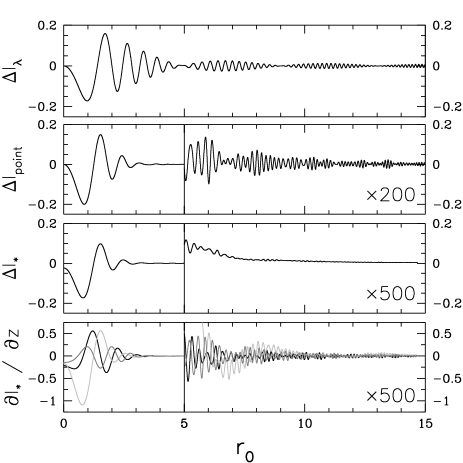
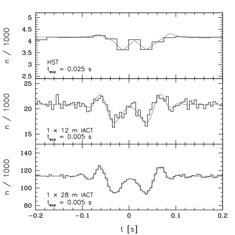
I show the expected light curves for the fiducial event in Figure 3. Note that the ringing in the monochromatic point-source diffraction pattern is suppressed by integration over wavelength and then by integration over the star’s disc. I also show a realization of the light curve with random noise (both Poisson and scintillation, treated as Gaussian white noise; Section 2.4) added as viewed by HST (top), a single 12 meter IACT as used in VERITAS (middle), and a single 28 meter IACT as used by HESS (bottom). The diffraction fringes are clearly detected by the IACTs. Note that I use a finer time resolution for the IACTs (200 Hz) than is possible with Hubble (40 Hz). Also note that IACTs have multiple telescopes, enhancing the signal further.
For comparison purposes, I also consider a “bright” star with , spectral type B5V, and .
3 Which Events are Detectable?
3.1 Detectability Using Matched Filters
N07 included the most extensive discussion of the detectability of TJO occultations. They defined a detectability statistic that is basically the deviation of from 1 integrated over time in units of a Fresnel-crossing time. Then if the event occurs over time bins, has a mean , after defining as the number of photons in time bin and as the expected number of photons when there is no event. The chance that the variations in the photon count rate are as large as the observed in the signal can then be estimated by noting that has a mean and variance of if no occultation occurs.
The N07 statistic provides a robust and conservative method of detecting any abnormally large fluctuation in the count rate, but it is not optimized for TJO occultations specifically. Occultations produce a characteristic ringing structure in the light curve, with changing smoothly from moment to moment. In contrast, the vast majority of signals that the statistic can detect are essentially noise with abnormally big variance and no time structure at all. The method loses statistical power by searching for a vast set of possible signals, of which occultations events are a tiny subset. This is reflected in the dependence of on ; the statistic actually decreases as the sampling rates passes due to the greater number of possible signals.
We optimize the signal-to-noise ratio for a known signal, in the presence of additive Gaussian white noise,555For a data series, the noise is white if the noise in each measurement is statistically independent. by applying a matched filter to the data (e.g., Davis89). Consider a series of data , where is an intrinsic signal we are interested in measuring, is additive white noise with constant variance, and averages to 0. If we wish to detect a known template pattern , we cross-correlate the observed data with a matched filter, which is simply itself: . The correlation is largest when the intrinsic signal matches the template signal . For an occultation, the data and the templates are the light curve of the background star (this is the cross-correlation method of Bickerton08). Note that both the data and template must be normalized so that the noise is constant (that is, the noise must be whitened).
Suppose we wish to detect a fluctuation in the star’s light curve. The renormalized data are
| (18) |
where is defined for telescope , is the ratio of the observed brightness of the star and its baseline brightness, and is the noise in the photon rate. For simplicity, I ignore variation in the noise rate during the event; this is valid for occultations with small depths. We cross-correlate with a template
| (19) |
to get the quantity:
| (20) |
Note that if there is no event (), the expectation value for is 0.
As long as the noise in each time bin is uncorrelated and has a normal distribution, itself is normally distributed. The expected variance of is
| (21) |
The effective signal-to-noise ratio (SNR) is then just . The signal is detected with significance level if
| (22) |
The cost of the matched filter approach is that the actual parameters of the occultation patterns are unknown, so a large number of templates must be tried. Therefore, we must set small to account for this look-elsewhere effect: essentially we must set to the reciprocal of the number of observations times the number of model occultation patterns. In order for the matched filter to work properly, the ringing of the template signal must be in phase with the ringing of the observed signal. The ratio of observing time to the duration of a single occultation event is (Lehner09). In addition, there are a number of parameters that must be fit: , , , , and . If there are 100 choices for each parameter, then there are possible templates. I thus set a threshold of , which requires .
3.2 Results
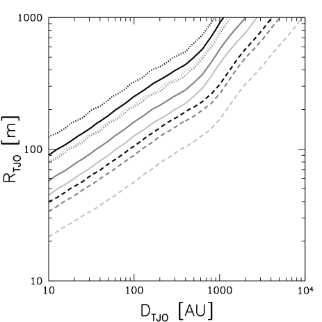
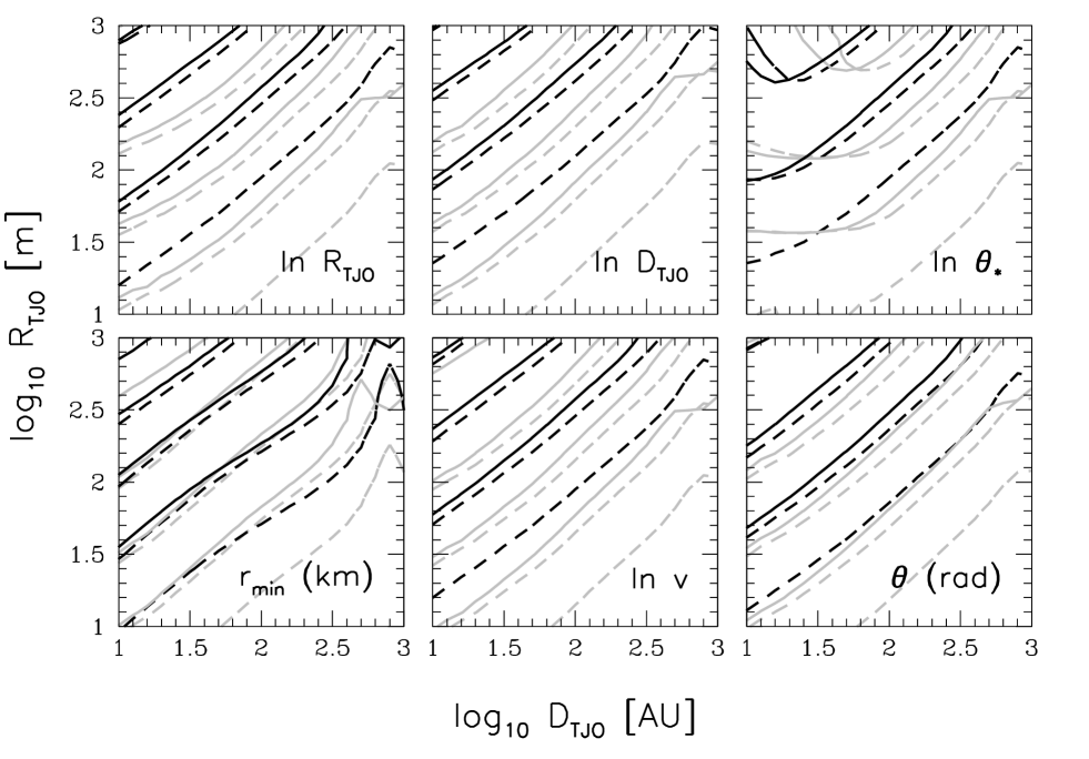
IACT arrays are excellent detectors of sub-kilometre TJOs. I show the limits on object radius and distance that can be detected with in Figure 4. For the occultations of “bright” B5V stars, VERITAS is able to detect objects as small as in radius 40 AU away, and 1 km radius objects out to 4000 AU (0.02 pc). Even for the less ideal A0V star, VERITAS can detect 200 meter radius objects 40 AU away and 1 km radius objects at 1000 AU (0.004 pc). But these limits pale compared to those for HESS, which has a large central telescope that can collect many photons and has relatively low scintillation noise. For the fiducial (bright) star, HESS can detect objects with () that are 40 AU away, and 1 km radius objects with (). The reach of CTA will be even more phenomenal. It is sensitive to occultations of the fiducial (“bright”) star by () objects 40 AU away and 1 km radius objects that are () away.
To put the sensitivities in perspective, what are the sensitivities of these arrays to the two TJO occultations observed with Hubble? These occultations, by objects roughly away (Schlichting09; Schlichting12), would have had SNRs of 63 (320) at VERITAS, 150 (430) at HESS, and 240 (1100) at CTA for the fiducial (“bright”) star. Likewise, the fiducial object has a significance of 31 (160) at VERITAS, 74 (220) at HESS, and 120 (550) at CTA when it occults the fiducial (“bright”) star.
Increasing the photon detection efficiency and decreasing the pixel size of the IACT detectors leads to strong improvements in their sensitivity to occultations of fainter stars. The use of “ideal” detectors improves the sensitivity of the IACT arrays to occultations of the fiducial star to those of the “bright” star. However, the “ideal” detectors do not improve sensitivity to occultations of the “bright” stars, because then the noise is dominated by scintillation.
So far, I have assumed the background star is A0V or B5V – as relatively nearby and blue star types, these stars have small angular diameters and therefore are well-suited for occultation detection (Table 2). The sensitivity to occultations of other star types is shown in Figure 4. As it turns out, all B to K dwarfs are roughly equally suitable for occultations: VERITAS is sensitive to occultations of dwarfs and CTA is sensitive to dwarfs by the fiducial object. In fact, O5V stars are actually worse than K dwarfs, because they are so strongly affected by dust extinction (Figure 2). Moving to the brighter giant stars, I again find that occultations of A to K dwarfs are roughly equally detectable, with slightly poorer sensitivity for B giants, and low sensitivity for M giants. The magnitude limits remain similar to dwarfs. But the sensitivities are especially poor for supergiants, where the sensitivity drops by several magnitudes. The best sensitivity for occultations of supergiants are when the supergiants are early type.
The diffraction pattern of an occultation need not pass through the core of an IACT array; it may pass some distance away, with a larger , so that only the outer fringes are detected by the IACT array. Yet the IACT array can still detect the occultation from the outer fringes alone. In Figure 5, I show how the detection significance varies with for the fiducial occultation. The significance is essentially constant as long as . At larger distances, the significance falls off exponentially as only the outer fringes are detected. But even then the IACTs can still detect diffraction patterns that pass several kilometres away, depending on the depth of the event, simply because the light collecting power of the IACTs is so great.
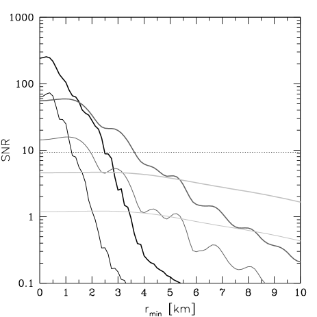
Intuitively, increases linearly with the number of photons collected during an event. Therefore, it scales inversely with the projected speed of the diffraction pattern. This is confirmed by an actual calculation.
For comparison, the limits of detectability using the N07 statistic are plotted as the dotted lines in Figure 4. I choose a time bin of , and I set the threshold at (N07). As expected, the power of the IACTs is weakened using this statistic. In fact, CTA is no more powerful than HESS, since it uses more telescopes, meaning more observations and more degrees of freedom. The fiducial event is still detectable even with VERITAS, so the ability of Cherenkov telescopes to find Kuiper Belt objects of this statistic seems robust.
4 Parameter Estimation with IACTs
4.1 Fisher matrices
The expected covariance matrix for estimated parameters of an experiment can be predicted beforehand by calculating its Fisher matrix (for a previous example of Fisher matrices applied to TJO occultations, see Cooray03-Fisher). Suppose an experiment makes measurements , with the -th measurement having an rms error of . It is fit by a model with parameters . Given the particle derivatives of the expected observed values with each parameter, the Fisher matrix is constructed as:
| (23) |
where and are in the range 1 to . The expected covariance matrix is just the inverse of the Fisher matrix, with for parameters and .
To calculate the Fisher matrix, we need the partial derivative of with each parameter. The function varies only if , , or varies; therefore the partial derivatives we need can be constructed from , , and . The formulae for two of the derivatives for a monochromatic point source are given in Appendix LABEL:sec:Derivations. Then, again assuming that the star’s spectrum is constant across its surface, we can first integrate over wavelength:
| (24) | ||||
| (25) |
and then over the star’s surface:
| (26) | ||||
| (27) |
Finally, the derivative with respect to stellar radius is found by differentiating equation 12:
| (28) |
4.1.1 Theorist’s parameter set
Between the observing geometry and the diffraction pattern, my model has seven unknown parameters. There is some freedom in choosing which seven variables stand in for these parameters. From a theoretical perspective, we are interested in the physical properties of the occulter, such as its distance, size, and speed. I first consider a set of “theorist’s” parameters – , , , , , , – explained below.
The partial derivatives are calculated by assuming that the other variables in the parameter set are kept constant. For example, suppose we had a set of two parameters, . Then is calculated assuming (and thus ) is constant. A pure increase in , with fixed, means that the TJO is bigger, because decreasing the distance would affect too. But if I used instead of , I would calculate assuming that is constant: a pure increase in for this parameter set means the TJO is closer, because changing the size would affect as well. It is like partial derivative in thermodynamics, where one must specify which variables are being held constant.
The first four variables relate solely to the observing geometry: , , , and . None of these depends on the Fresnel-scaled size of the occulter or the star; all can be expressed in terms of :
| (29) | ||||
| (30) | ||||
| (31) | ||||
| (32) |
These derivatives of follow simply from the Chain Rule. The next two parameters to be fit are the size of the body and the angular size of the star. The body’s radius is simply times the Fresnel scale. Since is independent of , there is no dependence on or , so that:
| (33) |
Likewise, the angular size of the star solely depends on : . This gives
| (34) |
Finally, the distance is unknown. All three of the variables , , and that determine the value of are physical quantities scaled by , which in turn depend on the distance. Therefore, by the Chain Rule, we have
| (35) |
4.1.2 Observer’s parameter set
The theorist’s parameter set is not the best formulation from an observational point of view. What the IACTs can actually measure is the duration of the event, the size of the Fresnel pattern, and the shape of the light curve (which depends on and ). These are essentially independent of one another, and should have small covariances. I therefore consider a set of observer’s parameters. The first three are , , and , as before. Then we have , , , and . As with the theorist’s variables, I calculate the partial derivatives with respect to each parameter using the Chain Rule.
The partial derivatives for , , and have the same values as for the physical parameter set. The partial derivatives and are also the same as those calculated in the beginning of the section. The remaining variables and do not depend on the size of the object or the star. They are
| (36) | ||||
| (37) |
4.2 Fisher matrix results
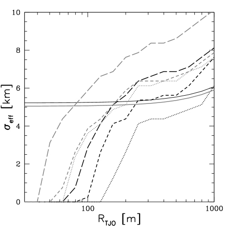
Although one potential advantage of IACT arrays is breaking degeneracies in parameter fitting, not every detectable event is tightly constrained. Figure 6 shows the precision IACT arrays can reach for each theorist’s parameter for TJOs of different sizes and distances. I find that the precision drops rapidly with distance. Note that occultations of “bright” stars improve parameter estimation precision by an order of magnitude (grey lines); therefore these occultations are the best chance that VERITAS and HESS have of measuring the physical properties of TJOs. Roughly, the precision increases by a factor of 10 if is 3 times bigger or is 3 times smaller. The exception is , for which the precision becomes smaller as decreases below for kilometre-sized objects.
| Parameter | Units | True | VERITAS | HESS | CTA | |||
| Value | Fiducial | “bright” | fiducial | “bright” | fiducial | “bright” | ||
| Theorist’s parameters (Fisher matrix) | ||||||||
| km | 0 | 0.097 | 0.0066 | 0.094 | 0.0065 | 0.011 | ||
| 30 | 9.5 | 0.65 | 6.6 | 0.45 | 0.24 | 0.016 | ||
| deg | 0 | 12 | 0.83 | 13 | 0.86 | 0.58 | 0.040 | |
| ms | 0 | 0.42 | 0.029 | 0.15 | 0.011 | 0.11 | 0.0076 | |
| m | 316 | 100 | 7.0 | 70 | 4.8 | 3.1 | 0.23 | |
| AU | 39.8 | 25 | 1.7 | 18 | 1.2 | 0.62 | 0.042 | |
| 14.0 (10.9) | 4.4 | 0.24 | 3.1 | 0.17 | 0.25 | 0.022 | ||
| Observer’s parameters (Fisher matrix) | ||||||||
| km | 1.27 | 0.42 | 0.028 | 0.29 | 0.019 | 0.010 | ||
| 23.6 | 0.19 | 0.013 | 0.079 | 0.0050 | 0.050 | 0.0034 | ||
| … | 0.248 | 0.0059 | 0.0024 | 0.0015 | ||||
| … | 0.316 (0.247) | 0.022 | 0.0018 | 0.0092 | 0.0058 | |||
: The first true value is for the fiducial A0V star with ; the value in parentheses is for the bright B5V star with .
I list the projected marginalized uncertainties on each parameter in Table 4 for the fiducial and bright star occultations. VERITAS and HESS can measure , , and precisely. The projected errors in , , , and are roughly 1/3 the actual values. Switching to observer’s parameters, the reason for the low accuracy is clear: although , , and are measured very precisely, itself can be measured only to 1 part in 3. Thus, even though an event is cleanly detected (with an SNR of 60 in this case), only vague inferences about the TJO’s properties can be derived.
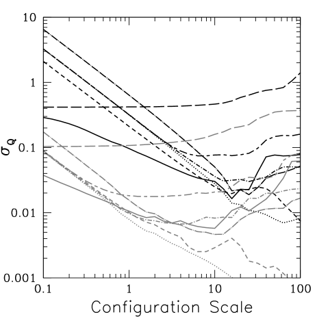
In fact, the typical baselines in VERITAS and HESS are , but the Fresnel scale for an object 40 AU away is over 1 km wide. I show what would happen if the spacings in the VERITAS array were multiplied by a constant scale factor in Figure 7. If VERITAS were ten times larger, it would be roughly the size of the Fresnel scale and could measure most of the occultation parameters precisely for . Despite this limitation, VERITAS and HESS should do well for occultations of bright stars, like the “bright” B5V stars, simply because there are more photons (upper right in Figure 8). In these cases, the errors become small enough to constrain the TJO speed, distance, and size to within 10%.

The error ellipses for each pair of theorist’s parameters for the “fiducial” occultation are plotted in Figure 8 for VERITAS. The covariances in the parameters are relatively small for this simulated event, except between the speed, radius, distance, and stellar angular radius, where the errors are highly correlated: an occultation may be by a small, close, slow object in front of a small star or a big, far, fast object in front of a large star. Note that, when the background star is A0V (bottom left), the Fisher matrix analysis indicates that the 3 confidence ellipses include regions of parameter space where the speed, distance, or radius of the TJO is 0! Of course, the Fisher matrix analysis is only accurate when the errors in the parameters are much smaller than the parameters themselves – the very fact that an occultation is detectable means the radius cannot be 0 (see the next section).
One way to break the degeneracy is if the stellar angular radius is independently known (cf., Cooray03-Fisher). Although VERITAS and HESS are too small to measure the pattern size, they can measure and accurately (Table 4). By combining prior knowledge of with a derived , one can calculate the distance of the TJO, and from there, the Fresnel scale, , and . Using a restricted Fisher matrix where is not counted as a free parameter, I find that VERITAS and HESS are much more powerful at estimating the object’s properties if is exactly known. Specifically, for the fiducial occultation, VERITAS (HESS) estimates to (), to (), and to ().
Another way to improve the parameter estimates is if is smaller, as is the case at quadrature instead of opposition. Then the theoretical light curve is the same, except that the event is longer. From the Fisher matrix, we see that the parameter variances scale as , or for the speed. So, for , the parameter errors are times smaller, except that is measured times more precisely. For the fiducial occultation, this alone is enough to estimate to 10 AU, to 40 metres, and to with VERITAS. The price is that occultation events occur more rarely when is small (Section 5).
According to the Fisher matrix analysis, CTA will have impressive capabilities in characterizing TJOs (Figure 6). The sizes and distances of TJOs occulting a fiducial star can be measured to within 10%, for 1 km radius objects 300 AUs away, or for 100 metre radius objects in the Kuiper Belt. When CTA observes an occultation of a bright star, it will be able to derive meaningful constraints even for kilometre-radius objects 2000 AU away, or 50 metre radius objects in the Kuiper Belt. As seen in Table 4, most of the improvement for distance is in measuring ; there are small gains in the precision of , , and compared to HESS.

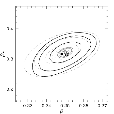
I show a projected set of error ellipses for the fiducial occultation at CTA in Figure 9. Even when observing the fainter fainter star, CTA is capable of constraining the object’s parameters to within a few percent. Although the errors between the TJO speed, radius, and distance are still correlated, the covariances are not as extreme as with VERITAS. Although many of CTA’s baselines are 100 m long, it also includes other baselines spanning up to 3.5 km (Table 1). Thus, it is larger than the Fresnel scale of a Kuiper Belt object and can measure the size of the diffraction pattern relatively well. Indeed, I show in Figure 7 that the E configuration of CTA already approximately has the optimal scale for estimating parameters from Kuiper Belt occultations. Of course, occultations of bright stars yield even more precise parameter estimates. For example, according to the Fisher matrix analysis, the radius of the fiducial object can be estimated to within 22 cm. Naturally, the model itself cannot be this accurate (Section 4.4).
Although the planned CTA is well spaced for observing Kuiper Belt Object occultations, it is not well-suited for characterizing objects in the Oort Cloud, simply because the Fresnel scale for these objects is so large. To improve its parameter estimation capabilities, additional telescopes must be added at a distance of . Distant telescopes could prove useful not only for Oort Cloud occultation observations, but for stellar intensity interferometry, another postulated use of the vast photon collection abilities of the array (LeBohec06; Dravins13).
4.3 Likelihood ratio estimation of parameters for the fiducial model
The projected confidence ellipses include unphysical values according to the Fisher matrix analysis, and a more accurate uncertainty projection is necessary. A fundamental tool in evaluating models is likelihood. The likelihood of a model is simply the probability of the data having its observed values under the assumption that the model is true:
| (38) |
for a data vector and a parameter vector . If the data are independent of each other, then the likelihood is the product of the probabilities for each data point. The parameters can be estimated by finding the model with the maximum likelihood.
We can quantify how well a model fits by taking the ratios of likelihoods:
| (39) |
Confidence bounds can be set by selecting regions in parameter space with above some threshold. According to Wilks’ theorem, tends to have a distribution where the number of degrees of freedom is the number of parameters in the model (e.g., Cash79). The confidence region is given by , the contour is given by and so on.666I checked whether the integrated posterior probability densities within these contours actually had the values of for , for , and for . They usually were in rough but not perfect agreement; for example, only % of the posterior probability density is within the 1 contour for with VERITAS. These disagreements may simply be due to the coarseness of the grid. The Fisher matrix method actually is a simplified case of the likelihood method, which approximates the likelihood as a second-order Taylor series around .
I estimate the likelihoods at each by assuming that each measurement has a value equal to the expected number of photons and a variance of (equation 17). I also assume that the probability distribution of is Gaussian; since the number of photons is large, this should be roughly correct. Then the log-likelihood is
| (40) |
| Parameter | VERITAS | CTA | ||
|---|---|---|---|---|
| Range | Step | Range | Step | |
| 0.9 – 1.1 | 0.01 | 0.975 – 1.025 | 0.0025 | |
| 0.5 – 1.5 | 0.05 | 0.9 – 1.1 | 0.01 | |
| 0.95 – 1.05 | 0.01 | 0.99 – 1.01 | 0.002 | |
| -0.7 – 2.0 | 0.1 | … | … | |
| … | … | 0.97 – 1.03 | 0.006 | |
| -2.0 – 2.0 | 0.4 | -0.4 – 0.4 | 0.08 | |
| -50 – 50 | 10 | -2.5 – 2.5 | 0.5 | |
| -0.4 – 0.4 | 0.08 | -0.04 – 0.04 | 0.008 | |
The parameter space has seven dimensions, so there is a very large combination of possible values even for one event. My approach is simply brute force: I calculate likelihood values on a full 7D grid with points (see Table 5 for details). I focus on the fiducial event so that the task is manageable. Brute force methods have been occasionally used before for estimating cosmological parameters (e.g., Efstathiou99; Tegmark00). For larger problems with more events or more parameters, though, a Markov Chain Monte Carlo method or high-order expansions of Fisher matrices (Sellentin14) may be employed more economically. In order for brute force to work effectively, the grid must be fine enough to sample with large inside each confidence region. The theorist’s parameter set is unsuitable because of the large covariances between variables; the confidence regions are “tilted” and slip through a square grid unless a huge number of points are used. Instead, I use the observer’s parameter set.
The resulting confidence bounds are 7D subsets of parameter space, but generally we wish to know the confidence region for just one or two of those parameters. We must marginalize the likelihoods: to compute the marginal likelihoods of a subset of the original parameter set, we integrate over the remaining parameters :
| (41) |
Likelihood marginalization is implicitly a Bayesian procedure, and requires a prior over the parameters that are integrated out (e.g., Freeman99). I assume flat uniform priors for all of the natural parameters (cf., Efstathiou99).
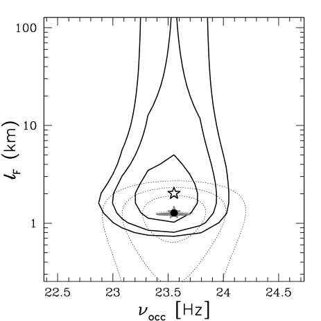
The coarseness of the grid limits the precision of the uncertainty estimates, but I find that the projected 1 marginalized uncertainties are comparable to those found with the Fisher matrix formalism. The exceptions are for , for which the uncertainties are times bigger than the Fisher matrix uncertainties, and , which has very weak upper bounds only. Some projected uncertainty ellipses for the fiducial model are shown in Figure 10. I find that the sizes of the confidence ellipses found with the Fisher matrix method (dotted) are similar to the regions found with the likelihood ratio method (solid), except when estimating . Although VERITAS can set a lower bound on the Fresnel scale, it cannot effectively distinguish between models with Fresnel scales that are much bigger than the array. As expected from the discussion in Section 4.2, CTA can constrain all parameters effectively for the fiducial occultation.
One minor difference with the fiducial model is that the maximum likelihood parameter set (stars in Figure 10) is not the same as the true parameter set (big dots). As a result, the confidence regions are shifted away from the true parameter set to some extent.
4.4 What else might be measurable?
The Fisher matrix analysis results in some extremely precise parameter estimates, especially with the CTA. But although the Fisher matrix analysis implies high precision for a given model, that does not mean the model is accurate. In fact, the models I use are highly idealized.
One assumption that may be relaxed is that of a perfectly spherical TJO. Roques87 discussed the diffraction patterns of nonspherical bodies. For an object larger than the Fresnel scale, the pattern is simply a geometrical shadow, and the TJO’s shape can be inferred by the time that the star is obscured at each telescope (as done for larger asteroids and TJOs). For objects smaller than the Fresnel scale, the shape of the object does not affect the size of the diffraction pattern. But Roques87 shows that the shape of the object affects the “ringing” of the diffraction pattern. There has not been a thorough study of how the ringing depends on shape, but it potentially encodes information that IACTs can exploit to infer the object shape. Young12 demonstrated how the diffraction pattern of the Schlichting09 TJO varies with oblateness. The different shapes in fact break the pattern’s radial symmetry, as well as affecting the details of the ringing. As IACT arrays can probe the two dimensional structure of diffraction patterns, they might constrain TJO shape. Detailed studies of their performance can be studied with the methods of Roques87 or Young12.
The other obvious idealization in the model is the assumption of a perfectly spherical and uniform background star. Real stars deviate from these assumption in three major ways. First, they can be oblate due to their rapid rotation. Secondly, they are limb-darkened, with the centre of the stellar disc appearing hotter and brighter than the edges. Finally, they can have large starspots.
5 Frequency of Occultations at Cherenkov Telescopes
A calculation of the event rate requires the sensitivity of the IACT array to a given event, the number of target stars, and a rate distribution for each event.
There are many distinct populations of TJOs. These span a vast range of sizes, ranging from dust grains to Pluto and Eris. The size distribution of a population of TJOs is often described by a broken power law. At larger radii, the number of objects increases extremely steeply as the radius decreases. But at some scale, the size distribution function turns over, and the number of objects increases more slowly as radius continues to decrease, with . The turnover to a spectrum has been seen in populations including Kuiper Belt objects and irregular satellites (Sheppard06-Moons; Schlichting12).
The volume filled by a population can also cover a large range in distances: the Centaurs range from 10 to 30 AU away, and the Oort Cloud may reach from 3000 to AU away. I assume that the distance distribution function is a power law truncated at a minimum and maximum distance and .
Nor are the TJOs necessarily evenly distributed across the sky. The simplest possible assumption is that they uniformly cover some solid angle . Observations generally constrain the integrated number of objects with radii above some value that is smaller than the power law break. The number of these objects per unit solid angle is . Combining the distance and size dependences, the normalized distribution function of a TJO population is
| (42) |
We can think of the diffraction patterns as moving around on the celestial sphere, each covering a small part of it. Then the rate of detectable occultations of a given star is
| (43) |
I use , appropriate for TJOs at opposition. The effective cross section of the diffraction pattern is the width of the parts of the pattern that are detectable:
| (44) |
Note that it is not in general equal to, for example, the Fresnel scale or the cross section given in N07, because IACT arrays are sensitive to the outer fringes of the diffraction pattern. I plot the effective cross sections to an occultation by the fiducial object as observed by the IACT arrays in Figure 11. The reach values that are about twice as high as the N07 width. Since depends on the detectability of the outer fringes, it depends on the magnitude and type of the observed star, and which IACT array is observing.
IACT arrays have wide fields of view, typically containing hundreds of stars, so the event rate observed by the IACT array is
| (45) |
where is the number of stars per unit solid angle and is the IACT field of view. Formally, I need to integrate over stellar magnitude, type, and extinction. I consider a simpler approximation with two populations of stars: those with , and those that are comparable to the “bright” star. For the former case, I assume that the sensitivity of IACTs to the fiducial star is typical of a star. I justify this by noting that the sensitivity of IACT arrays is comparable for dwarfs and giants earlier than K type (Figure 4). In addition, I compare to the stellar angular size distribution derived by Cooray03-Rates. They find that roughly half of stars have an angular radius that is less than , or twice the angular radius of the fiducial star.
The second case of the “bright” stars is more complicated, since B5V stars are at the small-angular size tail of the angular size distribution. According to the Cooray03-Rates model, essentially no stars have angular sizes that small. Only about 1 in 15 are less than twice as big as viewed from Earth. On the other hand, the optimal sensitivity to these stars is not just because of their small size, but also their low extinctions, which allows through the blue light that PMTs are most sensitive to. I simply divide the total number of stars brighter than by 15 to arrive at the number of “bright” stars, but a more rigorous model is desirable.
The integrated number of stars brighter than each magnitude as a function of Galactic latitude is given in Bahcall80. I use the worst case of the Galactic Poles, but note that the density at is times larger (Bahcall80). There are ten stars per square degree, and “bright” stars per square degree. I adopt a field of view of and assume that the sensitivity is uniform across the field, although angular resolution actually degrades towards the edges.
I list the expected occultation rates for several populations of TJOs in Table 6.
| Population | Distribution | VERITAS | HESS | CTA | |||
|---|---|---|---|---|---|---|---|
| “bright” | “bright” | “bright” | |||||
| KBOs | S12, | 10 | 100 | 4 | 80 | 2 | 20 |
| Centaurs | S00, | 700 | 7000 | 200 | 5000 | 100 | 1000 |
| S00, | 60 | 400 | 10 | 200 | 7 | 50 | |
| Scattered-Disc Objects | T00, | 300 | 2000 | 90 | 2000 | 50 | 500 |
| Oort Cloud Core | C13, | 20000 | 100000 | 6000 | 90000 | 3000 | 30000 |
| C13, | 1000 | 5000 | 300 | 3000 | 100 | 800 | |
| Hills (Oort) Cloud | O10, | … | … | 400000 | 500000 | 70000 | |
| O10, | … | 800000 | … | 300000 | 400000 | 50000 | |
| Uranus Trojans | A13, | 60000 | 500000 | 20000 | 400000 | 9000 | 100000 |
| A13, | 5000 | 30000 | 1000 | 20000 | 600 | 5000 | |
| Neptune Trojans | S10, | 300 | 2000 | 90 | 2000 | 50 | 500 |
| S10, | 20 | 90 | 4 | 60 | 2 | 10 | |
| Uranus Outer Satellites | S06 | 900 | 9000 | 300 | 6000 | 100 | 2000 |
| 600 | 5000 | 200 | 4000 | 90 | 1000 | ||
| 80 | 500 | 20 | 300 | 9 | 70 | ||
| Neptune Irregular Satellites | S06 | 2000 | 10000 | 500 | 10000 | 300 | 3000 |
| 200 | 2000 | 70 | 1000 | 40 | 400 | ||
| 20 | 100 | 5 | 70 | 2 | 20 | ||
I assume a field of view of for all telescopes. I also assume that occultations of all stars are as detectable as for a , A0V star, and that 7% of all occultations of stars are as detectable as for a , B5V star.
S12: Schlichting12; S00: Sheppard00; T00: Trujillo00; C13: Chen13; O10: Ofek10; S06: Sheppard06-Moons; S10: Sheppard10-NTrojanSizes; A13: Alexandersen13