Microscopic magnetic modeling for the $S$ = $\frac{1}{2}$ alternating chain compounds Na₃Cu₂SbO₆ and Na₂Cu₂TeO₆

Abstract

The spin-1/2 alternating Heisenberg chain system Na₃Cu₂SbO₆ features two relevant exchange couplings: $J_{1a}$ within the structural Cu₂O₆ dimers and $J_{1b}$ between the dimers. Motivated by the controversially discussed nature of $J_{1a}$, we perform extensive density-functional-theory (DFT) calculations, including DFT+$U$ and hybrid functionals. Fits to the experimental magnetic susceptibility using high-temperature series expansions and quantum Monte Carlo simulations yield the optimal parameters $J_{1a}\!=\!-217$ K and $J_{1b}\!=\!174$ K with the alternation ratio $\alpha=J_{1a}/J_{1b}\simeq-1.25$. For the closely related system Na₂Cu₂TeO₆, DFT yields substantially enhanced $J_{1b}$, but weaker $J_{1a}$. The comparative analysis renders the buckling of the chains as the key parameter altering the magnetic coupling regime. Numerical simulation of the dispersion relations of the alternating chain model clarify why both antiferromagnetic and ferrromagnetic $J_{1a}$ can reproduce the experimental magnetic susceptibility data.

I Introduction

The vibrant research on magnetic insulators keeps on delivering new examples of exotic magnetic behaviors and unusual magnetic ground states (GSs).Lee (2008); Balents (2010) Two prominent examples are the spin-liquid system herbertsmithite Cu₃Zn(OH)₆Cl₂, featuring a kagome lattice of $S\!=\!1/2$ spins,Helton et al. (2007) or the recently discovered Ba₃CuSb₂O₉, where the magnetism is likely entangled with the dynamical Jahn-Teller distortion.Nakatsuji et al. (2012)

Cuprates are a particularly promising playground to study low-dimensional magnetism, since they often combine the quantum spin $S\!=\!1/2$ ensured by the Cu $3d^{9}$ electron configuration and the low-dimensionality of the underlying magnetic model. The latter is ensued by the unique variety of lattice topologies realized in cuprates, which includes geometrically frustrated lattices, where quantum fluctuations are additionally enhanced by the competing magnetic interactions.

The simplest example of a quantum GS that lacks a classical analog is the quantum-mechanical singlet. Such a GS is found experimentally, e.g., in CsV₂O₅ (Ref. Isobe and Ueda, 1996; *csv2o5_valenti02; *csv2o5_saul11), CuTe₂O₅ (Ref. Deisenhofer et al., 2006; *cuteo_das08; *cuteo_ushakov09), CaCuGe₂O₆ (Ref. Sasago et al., 1995; *cacuge2o6_valenti02), and Cu₂(PO₃)₂CH₂ (Ref. Schmitt et al., 2010). All these compounds feature pairs of strongly coupled spins (magnetic dimers). An isolated dimer is an archetypical two-level quantum system, which can be solved analytically.

Compounds with sizable couplings between the dimers can exhibit diverse behaviors. For instance, the non-frustratedMazurenko et al. (2014) spin lattice of the Han purple BaCuSi₂O₆ is favorable for propagation of triplet excitations, promoting a Bose-Einstein condensation of magnons, experimentally observed in the magnetic field range between 23.5 and 49 T.Jaime et al. (2004); *bacusi2o6_sebastian06; *bacusi2o6_kraemer07 In contrast, SrCu₂(BO₃)₂ features strongly frustrated interdimer couplings that give rise to a fascinating variety of magnetization plateaus.*[][; andreferencestherein]SCBO_NMR_review The remarkable difference between the behavior of BaCuSi₂O₆ and SrCu₂(BO₃)₂ is governed by the difference in the magnetic couplings that constitute the respective spin model. Thus, the precise information on the underlying spin model is crucial for understanding the magnetic properties.

An evaluation of the microscopic magnetic model can be performed in different ways. The basic features of the spin lattice can be often conceived by applying empirical rules, such as the Goodenough–Kanamori rules.Goodenough (1955); *gka_2 Then, the resulting qualitative model is parameterized by fitting its respective free parameters to the experiment. The main challenge is the limited amount of the available experimental data that may not suffice for a unique and justified fitting of the model-specific free parameters. Thus, such a phenomenological approach is generally insecure against ambiguous solutions.

Microscopic modeling based on density-functional theory (DFT) calculations is an alternative solution. Such calculations require no experimental information beyond the crystal structure, and in contrast to the phenomenological method, provide a microscopic insight. A straightforward application of the DFT is impeded by the fact that cuprates are strongly correlated materials. Hence the effective one-electron approach of DFT generally fails to reproduce their insulating electronic GS.Pickett (1989) This shortcoming can be mended in alternative calculational schemes, such as DFT+$U$ or hybrid functionals, yet these methods are not parameter-free. Often, these parameters sensitively depend on the fine structural details of the system under investigation.

The low-dimensional $S\!=\!1/2$ Heisenberg compound Na₃Cu₂SbO₆ is an instructive example that demonstrates the performance and the limitations of the phenomenological as well as the microscopic approach. This compound was initially described as a distorted honeycomb lattice, owing to the hexagonal arrangement of the Cu atoms in the crystal structure.Miura et al. (2006) However, this purely geometrical analysis neglects the key ingredients of the magnetic superexchange, such as the orientation and the spatial extent of the magnetically active orbitals. Indeed, as pointed out by the authors of Ref. Miura et al., 2006, the orientation of the Cu $3d_{x^{2}-y^{2}}$ orbitals readily accentuates the chains formed by structural dimers and hints at two relevant magnetic couplings: $J_{\text{1a}}$ within the structural dimers and $J_{\text{1b}}$ between the dimers (Fig. 1), leading to the quasi-1D Heisenberg chain model with alternating nearest-neighbor couplings.

Thermodynamical measurements confirmed the quasi-1D character of the spin model,Miura et al. (2006); Derakhshan et al. (2007) yet no agreement was found for the sign of the intradimer coupling $J_{\text{1a}}$: Refs. Miura et al., 2006 and Derakhshan et al., 2007 vouch for a ferromagnetic (FM) and antiferromagnetic (AFM) exchange, respectively. The sign of $J_{\text{1a}}$ basically governs the magnetic GS: the AFM-AFM solution is a disordered dimer state, while the GS of an FM-AFM chain is adiabatically connected to the Haldane phase with nontrivial topology and sizable string order parameter.Yamanaka et al. (1993) Therefore, for the magnetic GS, the sign of $J_{\text{1a}}$ is of crucial importance.

Notably, even DFT studies do not concur with each other: Ref. Derakhshan et al., 2007 reports AFM $J_{\text{1a}}$, while an alternative DFT-based method in Ref. Koo and Whangbo, 2008 yields FM coupling. To resolve the controversy on the sign of $J_{\text{1a}}$, the authors of Ref. Miura et al., 2008 performed inelastic neutron scattering (INS) experiments on single crystals of Na₃Cu₂SbO₆. The resulting values for the exchange couplings ($J_{\text{1a}}$ = $-145$ K and $J_{\text{1b}}$ = 161 K) clearly indicate the FM-AFM chain scenario. Still, the origin of ambiguous solutions in earlier experimental as well as in DFT studies has not been sufficiently clarified.

In our combined experimental and theoretical study, we evaluate the magnetic model for Na₃Cu₂SbO₆ and its Te sibling Na₂Cu₂TeO₆ (Ref. Xu et al., 2005) using extensive DFT calculations and investigate how the magnetic GS is affected by the structural distortion within the chains. By comparing our DFT results to the earlier studies, we explain the origin of ambiguous parameterizations of DFT-based spin models in both compounds. Simulations of the momentum-resolved spectrum for our microscopic model reveal excellent agreement with the INS experiments (Ref. Miura et al., 2008) and enlighten the ambiguity of AFM–AFM and FM-AFM solutions inferred from the thermodynamical measurements.

This paper is organized as follows. The used experimental as well as computational methods are described in Sec. II. The details of the crystal structures of Na₃Cu₂SbO₆ and Na₂Cu₂TeO₆ are discussed in Sec. III. In Sec. IV, we present our magnetic susceptibility measurements and extensive DFT calculations. Peculiarities of the excitation spectrum of the Heisenberg chain model is discussed Sec. V. Finally, a summary and a short outlook are given in Sec. VI.

II Methods

Synthesis and sample characterization

Polycrystalline samples of Na₃Cu₂SbO₆ were prepared by solid state reaction. A stoichiometric amount of Na₂CO₃ (Chempur, 99.9+%), Sb₂O₅ (99.999%, Alfa Aesar) and CuCO₃$\cdot$Cu(OH)₂ (Chempur) was thoroughly mixed. The homogeneous powder was pressed into a platinum crucible and annealed at 1273 K for two weeks in air. Finally the crucible was taken out of the furnace at 1273 K and cooled down to room temperature in air.

For magnetic measurements, the powder sample was pressed into a pellet and heated again at 973 K in a platinum boat for several days. The green powder was identified and characterized by powder x-ray diffraction using a high-resolution Guinier camera with Cu K_α radiation. The determined lattice parameters $a\!=\!5.676$ Å, $b\!=\!8.860$ Å, $c\!=\!5.833$ Å and $\beta\!=\!113.33^{\circ}$ are in good agreement with Ref. Smirnova et al., 2005.

To control the oxygen content in the sample at different stages of the thermal treatment, we performed coulometric titration of the samples using a commercial OXYLYT device. We found that the maximal oxygen content (close to the stoichiometric Na₃Cu₂SbO₆) is attained right after the thermal treatment at 973 K (Fig. S3 in Ref. sup, ). However, a subsequent storage at room temperature and in air leads to a reduction of the oxygen content. This effect can be seen in the magnetic susceptibility by the increased amount of Curie impurity (Fig. S4 in Ref. sup, ). Therefore, for thermodynamic measurements, we use “fresh” samples (i.e., we performed measurement right after the thermal treatment) that feature smallest impurity contribution. Magnetic susceptibility $\chi(T)$ of Na₃Cu₂SbO₆ was measured using a SQUID magnetometer (MPMS, Quantum Design) in a magnetic field of 0.04 T.

DFT calculations

For the electronic structure calculations, the full-potential local-orbital code FPLO (version fplo8.50-32) within the local (spin) density approximation (L(S)DA) was used.Koepernik and Eschrig (1999) In the scalar relativistic calculations the exchange and correlation potential of Perdew and Wang has been applied.Perdew and Wang (1992) The accuracy with respect to the $k$-mesh has been carefully checked.

The LDA band structure has been mapped onto an effective one-orbital tight binding (TB) model based on Cu-site centered Wannier functions (WF). The strong Coulomb repulsion of the Cu $3d$ orbitals was considered by mapping the TB model onto a Hubbard model. In the strongly correlated limit and at half-filling, the lowest lying (magnetic) excitations can be described by a Heisenberg model with $J^{\text{AFM}}_{ij}\!=\!4t_{ij}^{2}/U_{\text{eff}}$ for the antiferromagnetic part of the exchange. Spin-polarized LSDA+$U$ supercell calculations were performed using two limiting cases for the double counting correction (DCC): the around-mean-field (AMF) and the atomic limit (AL, also called the fully localized limit). We varied the on-site Coulomb repulsion $U_{3d}$ in the physically relevant range (4–8 eV in AMF and 5–9 eV in AL), keeping the on-site exchange $J_{3d}\!=\!1$ eV.

The partial Na_3-x occupancy and the Sb_x/Te_1-x substitution were modeled using the virtual crystal approximation (VCA).Kasinathan et al. (2012)

HSE06 (Ref. Heyd et al., 2003; *HSE06) hybrid functional calculations were performed using the pseudopotential code vasp-5.2,Kresse and Furthmüller (1996a); *vasp2 employing the basis set of projector-augmented waves. The default admixture of the Fock exchange (25%) was adopted. We used the primitive unit cell with 2 Cu atoms and a 6$\times$6$\times$6 $k$-mesh with the NKRED=3 flag.

Simulations and fits to the experiment

We used the high-temperature series expansion (HTSE) to a Heisenberg chain with alternating nearest-neighbor couplings $J_{\text{1a}}$ and $J_{\text{1b}}$. For the case of AFM couplings, the parameterization is given in $\alpha\equiv|J_{\text{1a}}|/J_{\text{1b}}$ in Table II of Ref. Johnston et al., 2000; the parameters for the case of FM $J_{\text{1a}}$ are provided in Ref. Borras-Almenar et al., 1994. Quantum Monte Carlo simulations were performed using the loop algorithmTodo and Kato (2001) from the ALPS package.Albuquerque et al. (2007) To evaluate the reduced magnetic susceptibility, we used 50 000 loops for thermalization and 500 000 loops after thermalization for chains of $N\!=\!120$ spins $S\!=\!1/2$ using periodic boundary conditions. Exact (Lanczos) diagonalization of the Heisenberg Hamiltonians was performed using spinpack.Schulenburg The lowest-lying $S^{z}$ = 0, $S^{z}$ = 1 and $S^{z}$ = 2 excitations were computed for $N$ = 32 sites chains of $S$ = 1/2 using periodic boundary conditions.

III Crystal structure

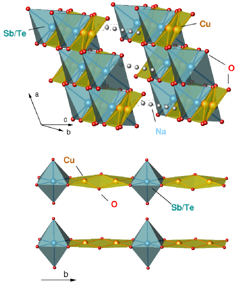
Figure 1: (Color online) Top: crystal structure of Na₃Cu₂SbO₆. The basic elements are CuO₄ plaquettes and SbO₆ octahedra. Bottom: segments of the structural chains of Cu₂O₆ dimers for the experimental distorted plaquette geometry (upper panel) and an ideal planar arrangement of the Cu₂O₆ units in the fictitious structures (lower panel).

The monoclinic (space group $C2/c$) crystal structure of Na₃Cu₂SbO₆ (Ref. Smirnova et al., 2005) features pairs of slightly distorted, edge-shared CuO₄ plaquettes forming structural dimers with the Cu–O–Cu bonding angle of 95 ^∘. The dimers are connected by the equatorial plane of SbO₆ octahedra and form chains running along the $b$ axis (Fig. 1, bottom). The apical O atoms of the SbO₆ octahedra mediate connections to the next Cu₂O₆ dimer chain. In this way, the magnetic layers, separated by Na atoms, are formed (Fig. 1, top).

The crystal structure of Na₂Cu₂TeO₆ (Ref. Xu et al., 2005) features a similar motif, with the reduced number of Na atoms between the layers, to keep the charge balance. In addition, the smaller size of Te⁶⁺ compared to Sb⁵⁺ gives rise to a stronger distortion of the Cu₂O₆ dimer chains in Na₂Cu₂TeO₆. To investigate the influence of this distortion, we also computed fictitious structures with idealized planar arrangements of the Cu₂O₆ units (Fig. 1 bottom, lower panel).

IV Results

IV.1 Magnetic susceptibility

Above 200 K, the magnetic susceptibility of Na₃Cu₂SbO₆ fits reasonably to the Curie-Weiss law with $C$ = 0.442 emu K(mol Cu)^-1 and the antiferromagnetic Weiss temperature $\theta_{\text{CW}}$ = 60$\pm$10 K. The effective magnetic moment amounts to $\mu_{\text{eff}}\!\simeq\!1.88$ $\mu_{\text{B}}$, slightly exceeding the spin-only value for $S$ = 1/2 (1.73 $\mu_{\text{B}}$). The resulting value of the Lande factor $g$ = 2.17 is typical for Cu²⁺ compounds. At lower temperatures, antiferromagnetic correlations give rise to a broad maximum in the magnetic susceptibility around $T_{\text{max}}$ = 96 K. The low-temperature upturn below 17 K is likely caused by defects, typical for powder samples of quasi-1D magnets $[$e.g., Sr₂Cu(PO₄)₂ from Ref. Belik et al., 2004 or (NO)Cu(NO₃)₃ from Ref. Volkova et al., 2010$]$, since already a single defect terminates the spin chain.

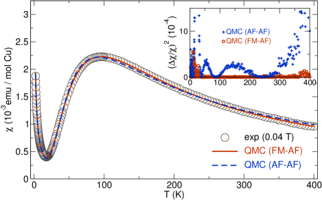
Figure 2: (Color online) Experimental (exp) magnetic susceptibility of Na₃Cu₂SbO₆ (circles) and the quantum Monte Carlo (QMC) fits for the FM-AFM and the AFM-AFM solution of the alternating Heisenberg chain (AHC) model. Inset: difference curves emphasize the excellence of the FM-AFM solution.

We briefly compare our susceptibility measurements with the published data. The Curie-Weiss fit from Ref. Derakhshan et al., 2007 yields a similar $\theta_{\text{CW}}$ = 55 K, but their $g$ = 2.33 exceeds our estimate. This discrepancy likely originates from the difference in the magnetic field (0.1 T versus 0.04 T in our work) as well as different temperature ranges used for the fitting. Unfortunately, the authors of Ref. Miura et al., 2006 do not provide the values of $\theta_{\text{CW}}$ and $g$, but a Curie-Weiss fit to their data yields $\theta_{\text{CW}}$ $\simeq$ 49 K and $g$ $\simeq$ 2.10, in good agreement with our findings. A bare comparison of the absolute values of $\chi(T_{\text{max}})$ (Table 1) reveals sizable deviations of the $\chi(T)$ data from Ref. Derakhshan et al., 2007 compared to the other two data sets.

Table 1: Na₃Cu₂SbO₆: the Curie-Weiss temperature $\theta_{\text{CW}}$ (in K) and the $g$-factor evaluated using the Curie-Weiss fit for $T\!\geq\!200$ K, as well as the experimental position $T_{\text{max}}$ (in K) of the susceptibility maximum and its abosolute value $\chi(T_{\text{max}})$ $[$in emu (mol Cu)${}^{-1}]$.

data source	$\theta_{\text{CW}}$	$g$	$T_{\text{max}}$	$\chi(T_{\text{max}})$
this study	60	2.17	96	2.2$\cdot 10^{-3}$
data from Ref. Miura et al.,2006	49	2.10	95	2.3$\cdot 10^{-3}$
Ref. Derakhshan et al.,2007	55	2.33	90	1.7$\cdot 10^{-3}$

For a more elaborate analysis, we adopt the AHC model and search for solutions that agree with the experimental $\chi(T)$ curve. To this end, we perform HTSE considering the physically different scenarios: both $J_{\text{1a}}$ and $J_{\text{1b}}$ couplings are AFM (“AFM–AFM”) and $J_{\text{1a}}$ is FM (“FM–AFM”). The corresponding HTSE coefficients for the two cases can be found in Refs. Johnston et al., 2000 and Borras-Almenar et al., 1994, respectively. In both cases, we obtain a solution (first row of Table 2) which conforms to the experimental data.

Table 2: High-temperature series expansion (HTSE) and quantum Monte Carlo (QMC) fits to the experimental $\chi(T)$ data for Na₃Cu₂SbO₆. Results of different studies implying a ferromagnetic and an antiferromagnetic coupling (FM-AFM, upper lines) or two inequivalent antiferromagnetic couplings (AFM-AFM, lower lines) are shown: exchange couplings $J_{\text{1a}}$ and $J_{\text{1b}}$ (in K), $g$-factors, temperature-independent terms $\chi_{0}$ $[$in emu / (mol Cu)${}^{-1}]$, and Curie-Weiss impurity contributions $C^{\text{imp}}$ $[$in K emu (mol Cu)${}^{-1}]$ and ${\theta}^{\text{imp}}_{\text{CW}}$ (in K). “$-$” stands for a fitted quantity, which numerical value is not provided in the respective reference.

	$J_{\text{1a}}$	$J_{\text{1b}}$	$g$	$\chi_{0}$	$C^{\text{imp}}$	${\theta}^{\text{imp}}_{\text{CW}}$
HTSE
this study	$-207$	171	2.01	3$\times 10^{-5}$	4.7$\times 10^{-3}$
	155	66	2.20	$3\times 10^{-6}$	6.1$\times 10^{-3}$	1.1
Ref. Miura et al.,2006	$-209$	165	2.01	$-$	$-$	$-$
	143	39	2.13	$-$	$-$	$-$
Ref. Derakhshan et al.,2007	160	62	1.97	2.2$\times 10^{-4}$		$2.3$
QMC
this study	$-$217	174	2.02	9$\times 10^{-6}$	6$\times 10^{-3}$	1
	153	61	2.19	3$\times 10^{-6}$	6$\times 10^{-3}$	1.2

Our solution for the FM-AFM case (Table 2, first row) nearly coincides with the corresponding solution from Ref. Miura et al., 2006 (Table 2, second row), yielding $\alpha\equiv{J_{\text{1a}}/J_{\text{1b}}}\!\simeq\!-1.25$ and a considerably smaller $g$-factor of about 2 compared to the value from the Curie-Weiss fits (2.17). For the AFM-AFM case, we obtain $\alpha\!\simeq\!0.4$ which deviates from the result of Ref. Miura et al., 2006, but closely resembles the solution from Ref. Derakhshan et al., 2007 (Table 2, third row). The discrepancy can originate from different parameterizations used for the HTSE fitting. In particular, the AFM-AFM solutions in Refs. Miura et al., 2006 and  Derakhshan et al., 2007 are obtained using the parametrization from Ref. Hall et al., 1981. In contrast, we adopt the coefficients from a more recent and extensive study,Johnston et al. (2000) valid in the whole temperature range measured.

To account for the full temperature range measured, we turn to QMC simulations. Thus, we adopt the ratios $\alpha\!=\!-1.25$ and $\alpha\!=\!0.40$ from our HTSE fitting, and calculate the reduced magnetic susceptibility $\chi^{*}(T/k_{B}J)$, which can be fitted to the experimental curve using the expression:

$$\chi(T)=\frac{N_{A}g^{2}{\mu}_{B}^{2}}{k_{B}J}\cdot\chi^{*}\biggl{(}\frac{T}{k_{B}J}\biggl{)}+\frac{C^{\text{imp}}}{T+\theta^{\text{imp}}_{\text{CW}}}+\chi_{0},$$ (1)

where $N_{A}$ and $k_{B}$ are the Avogadro and Boltzmann constants, respectively, $\mu_{B}$ the Bohr magneton, $C^{\text{imp}}$ and $\theta^{\text{imp}}_{\text{CW}}$ account for impurity/defect contributions, $\chi_{0}$ is a temperature-independent term, and $J=\max\{|J_{\text{1a}}|,J{{}_{\text{1b}}}\}$. Using a least-squares fitting, we obtain the solutions listed in Table 2 (last row) and shown in Fig. 2.

The AFM–AFM solution shows sizable deviations at high temperatures and in the vicinity of the low-temperature upturn (Fig. 2, inset), while the FM-AFM solution yields an excellent fit to the experimental $\chi(T)$ in the whole temperature range, making the latter solution more favorable. Still, the choice is impeded by the following issues. First, the AHC model is a minimal model for Na₃Cu₂SbO₆, which completely neglects interchain couplings and anisotropies. Second, the $g$-factor of the FM-AFM solution deviates significantly from the estimate based on the Curie-Weiss fit, while its counterpart from the AFM-AFM solution shows a better agreement with the Curie-Weiss fit. Finally, the shape of the $\chi(T)$ curve is affected by oxygen deficiency in the sample,sup which is difficult to control during the synthesis process. Therefore, the AFM-AFM solution can not be ruled out using the $\chi(T)$ data, only.

IV.2 Electronic structure and magnetic model

To resolve the ambiguity between the FM-AFM and AFM-AFM solutions, we perform microscopic magnetic modeling of Na₃Cu₂SbO₆ and its Te sibling Na₂Cu₂TeO₆ using DFT calculations. The valence bands feature similar band width and are similarly structured in the two compounds, as revealed by the LDA densities of states (DOS) in Fig. 3. The DOS is dominated by Cu and O states down to $-5.5$ eV and $-6$ eV for Na₃Cu₂SbO₆ and Na₂Cu₂TeO₆, respectively. Contributions from Na, Sb and Te are marginal in this energy range. Only at the lower edge of the valence band, we find a sizable hybridization of Sb states for Na₃Cu₂SbO₆ centered around $-6$ eV. A similar admixture of Te states is observed for Na₂Cu₂TeO₆, where the additional valence electron of Te compared to Sb shifts the Cu–O–Te density down by about 1 eV.

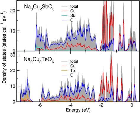
Figure 3: (Color online) Total and atom-resolved LDA density of states for Na₃Cu₂SbO₆ (top) and Na₂Cu₂TeO₆ (bottom). The contribution of Na states is negligible on this scale (not shown).

The LDA band structures for both compounds feature a well-separated density of Cu and O states centered around the Fermi energy. In the local coordinate system of a CuO₄ plaquette, this density is formed by the anti-bonding $\sigma$-combination of Cu $3d_{x^{2}-y^{2}}$ and O $2p_{\sigma}$ states ($dp\sigma^{*}$ combination). The orbital-resolved density of states for Na₃Cu₂SbO₆ is shown in Fig. 4. Two aspects should be pointed out. First, the metallic solution (nonzero DOS at the Fermi energy) observed in Na₃Cu₂SbO₆, is in contrast with the green color of the compound, indicative of the insulating behavior. Similar, the calculated LDA band gap of 0.06 eV for Na₂Cu₂TeO₆ (see Fig. 3) is far too small to account for the green color of the powder and originates from dimerization effects. This drastic underestimation of the band gap is a well-known shortcoming of the LDA, which does not account for the strong Coulomb repulsion in the Cu 3$d$ orbitals. The missing part of correlation energy will be accounted for by resorting to a Hubbard model, as well as using DFT+$U$ and hybrid-functional calculations. Second, the orbital resolved density of states (see Fig. 4) shows small hybridization with the out-of-plane Cu-O states due to the distortion of the dimer chains. Since these contributions are small compared to the pure antibonding $dp\sigma^{*}$ states, the restriction to an effective TB model is still justified.

To verify the structural input, we relaxed the crystal structures within LDA. For Na₃Cu₂SbO₆, the relaxation results in a rather small energy gain of 33 meV per formula unit (f. u.), and the respective changes in the crystal structure are negligible. In contrast, a relaxation of the atomic coordinates in Na₂Cu₂TeO₆ lowers the energy by 130 meV per f. u. and alters mainly the chain buckling. Since the relaxation of Na₂Cu₂TeO₆ affects the magnetically relevant $dp\sigma^{*}$ states, we evaluated the magnetic properties for both, the experimental and the relaxed crystal structure.

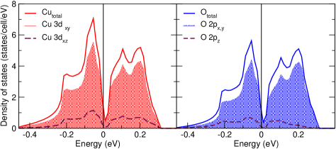
Figure 4: (Color online) Orbital-resolved LDA density of states for Na₃Cu₂SbO₆. In the local coordinate system of a CuO₄ plaquette, the $x$ axis runs along one of the Cu–O bonds, while the $z$ axis is perpendicular to the plaquette plane (for the ideal planar coordination). The states in the vicinity of the Fermi energy are dominated by the in-plane Cu $3d$ and O $2p$ states.

The transfer integrals $t_{ij}$ (the hopping matrix elements) are evaluated by a least-squares fit of an effective one-orbital TB model to the two LDA $dp\sigma^{*}$ bands. Using 10 inequivalent $t_{ij}$ terms (see the bottom panel of Fig. 5, Table 3, and Ref. sup, ) we obtain excellent agreement between the TB model and the LDA band structure. The respective fit for Na₃Cu₂SbO₆ is shown in Fig. 5 (top).

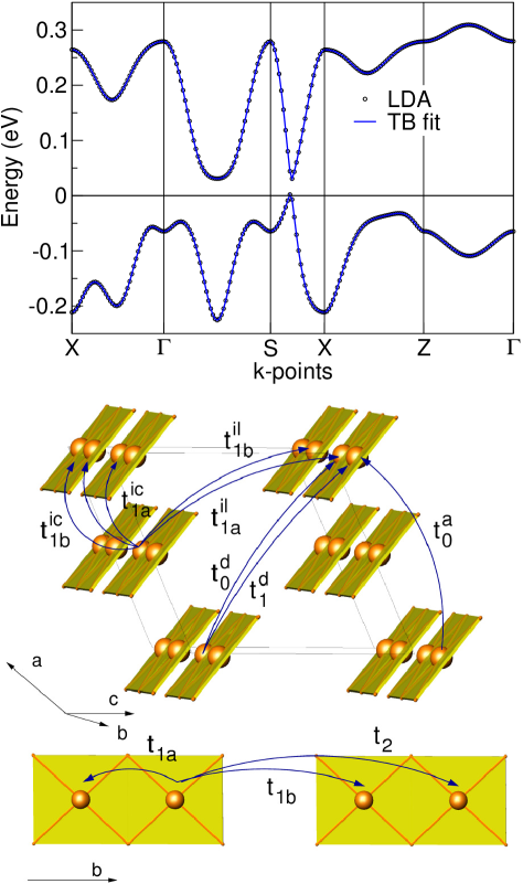
Figure 5: (Color online) Top: LDA band structure of Na₃Cu₂SbO₆ and the fit using the effective one-orbital TB model with ten inequivalent transfer integrals $t_{ij}$. Bottom: the superexchange pathways corresponding to the relevant $t_{ij}$ terms.

Table 3: Relevant ($>$10 meV) transfer integrals $t_{ij}$ (in meV) evaluated by fitting the LSDA band structures for the different structural models: experimental (exp), LSDA-relaxed (relaxed) and fictitious planar (planar). For the notation of $t_{ij}$, see Fig. 5 (bottom).

Na3Cu2SbO6
$t_{i}$/meV	$t_{1a}$	$t_{1b}$	$t_{2}$	$t^{ic}_{1a}$	$t^{ic}_{1b}$	$t_{0}^{d}$	$t_{0}^{a}$
exp	60.6	127	18.2	$-$27.8	17.0	21.8	17.4
relaxed	68.2	134	18.1	$-$32.3	20.6	20.9	19.2
planar exp	45.3	119	22.4	$-$7.8	9.4	30.1	$-$
planar relax.	55.6	125	23.8	$-$9.2	10.7	29.2	$-$
Na2Cu2TeO6
$t_{i}$/meV	$t_{1a}$	$t_{1b}$	$t_{2}$	$t^{ic}_{1a}$	$t^{ic}_{1b}$	$t_{0}^{d}$	$t_{0}^{a}$
exp	15.6	162	16.4	$-$38.5	24.7	13.7	25.5
relaxed	42.5	152	17.3	$-$42.4	26.3	14.5	23.1
planar exp.	27.3	152	29.3	$-$12.6	12.4	25.6	1.3
planar relax.	45.2	148	30.0	$-$12.8	12.7	26.0	$-$

In both systems, the leading coupling is $t_{1b}$, which connects two neighboring structural dimers: $t_{1b}\!=\!127$ meV for Na₃Cu₂SbO₆ and $t_{1b}\!=\!162$ meV for Na₂Cu₂TeO₆, respectively. The coupling within the structural Cu₂O₆ dimers ($t_{1a}\!=\!60$ meV for Na₃Cu₂SbO₆ and $t_{1a}\!=\!16$ meV for Na₂Cu₂TeO₆) are significantly smaller. Besides, several long-range couplings that connect different chains, are comparable to $t_{1a}$ (Table 3 and Ref. sup, ). Subsequent mapping of the TB model onto a Hubbard model (adopting $U_{\text{eff}}\!=\!4$ eV) and a Heisenberg model, yield the following AFM contributions: $J^{\text{AFM}}_{1b}\!=\!188$ K and $J^{\text{AFM}}_{1a}\!=\!43$ K for Na₃Cu₂SbO₆ and $J^{\text{AFM}}_{1b}\!=\!305$ K and $J^{\text{AFM}}_{1a}\!=\!2$ K for Na₂Cu₂TeO₆, respectively.

The resulting minimal model is incomplete, since it disregards the FM contribution to the exchange integrals, which are expected to be especially large for the $J_{1a}$ coupling within the structural dimers. To estimate the total exchange integrals, comprising AFM and FM contributions, we performed LSDA+$U$ calculations of magnetic supercells. Mapping the total energies of different collinear spin arrangements onto a classical Heisenberg model yields $J_{1a}\!=\!-135\pm 20$ K for Na₃Cu₂SbO₆ and $J_{1a}\!=\!-120\pm 20$ K for Na₂Cu₂TeO₆, respectively. For the exchange between the structural dimers, we find $J_{1b}\!=\!150\pm 50$ K for Na₃Cu₂SbO₆ and $J_{1b}\!=\!232\pm 70$ K for Na₂Cu₂TeO₆ ($U_{3d}\!=\!6\mp 1$ eV). All further exchange integrals between different chains and layers are smaller than 10 K, and thus can be neglected in the minimal model.

Unlike the related compounds featuring edge-shared chainsSchmitt et al. (2009); Wolter et al. (2012) or Cu₂O₆ dimers,Schmitt et al. (2010) Na₃Cu₂SbO₆ and Na₂Cu₂TeO₆ exhibit a sizable influence of the Coulomb repulsion $U_{3d}$ on the exchange integrals (see Fig. 6). However, the variation of $U_{3d}$ within the physically relevant range (Sec. II) does not affect the FM nature of $J_{1a}$. Thus, Na₃Cu₂SbO₆ features alternating chains with the exchange integrals of nearly the same magnitude but different sign (FM $J_{1a}$ and AFM $J_{1b}$), while for Na₂Cu₂TeO₆, the AFM exchange between the structural dimers is dominant. The evaluated exchange integrals are listed in Table 4.

For an independent computational method, we use hybrid functional (HF) total energy calculations. The absence of the double counting problem and minimal number of free parameters makes HF calculations an appealing alternative to the DFT+$U$ methods.Fuchs et al. (2007) Here, we employ the HSE06 functional to evaluate the leading couplings $J_{1a}$ and $J_{1b}$ in both compounds. In accord with DFT+$U$, we obtain FM $J_{1a}$ and AFM $J_{1b}$. For Na₃Cu₂SbO₆, the resulting exchange integrals are in excellent agreement with the HTSE estimates (Table 4). Similar to DFT+$U$, Na₂Cu₂TeO₆ features a weaker $J_{1a}$ and stronger $J_{1b}$, thus the $\alpha$ value is substantially reduced.

We are now in position to compare our results with the previous DFT-based studies. Derakhshan et al. (Ref. Derakhshan et al., 2007) evaluated the relevant transfer integrals using $N$th-order muffin-tin-orbital downfolding of the LDA band structure. Although this computational method (Ref. Andersen and Saha-Dasgupta, 2000) as well as the codeAndersen and Jepsen (1984) used for the calculations differ from our approach, the difference in the resulting $t_{ij}$ values does not exceed 25%.[DifferentDFTcodesemploydifferentbasissets; hencetheresultingbandstructuresarenotidentical.Foraninstructiveexample; see][]SCPO_comment Hence, the estimated AFM contributions to the exchanges $J_{1a}$ and $J_{1b}$ generally agree with our values. However, in contrast to the present study, the authors of Ref. Derakhshan et al., 2007 did not perform DFT+$U$ calculations and therefore completely disregarded the FM contributions, which are especially relevant for the short-range coupling $J_{1a}$. Thus, their AFM-AFM solution originates from a severe incompleteness of the computational scheme and the respective mapping onto the spin Hamiltonian.

In contrast to Ref. Koo and Whangbo, 2008, Koo and Whangbo performed DFT+$U$ calculations using vasp, and recovered FM $J_{1a}$ and AFM $J_{1b}$, in qualitative agreement with the experiment. However, the absolute values of the leading couplings are considerably overestimated. We believe that this overestimation stems from the choice of the on-site Coulomb repulsion parameter $U_{d}$. It is well-known that the parameters of the DFT+$U$ calculations are not universal,Ylvisaker et al. (2009) in particular basis dependent, and should be carefully chosen based on the nature of the magnetic atom and the code used. The $U_{d}$ range studied in Ref. Koo and Whangbo, 2008 (4..7 eV) is too narrow, and larger $U_{d}$ is likely required to reproduce the correct magnetic energy scale in Na₃Cu₂SbO₆ and Na₂Cu₂TeO₆.

Table 4: Leading exchange integrals $J_{1a}$ and $J_{1b}$ (in K) and the alternation ratio $\alpha\!\equiv\!J_{1a}/J_{1b}$ for Na₃Cu₂SbO₆ and Na₂Cu₂TeO₆, evaluated using different methods. HTSE and QMC estimates are made based on the experimental data from the respective reference (first column). Theoretical estimates, LSDA+$U$, HSE06, and extended Hückel tight-binding (EHTB) are based on calculations for the experimental crystal structures.

data source	method	$J_{1a}$	$J_{1b}$	$\alpha$ = $J_{1a}$/$J_{1b}$
Na3Cu2SbO6
this study	LSDA+$U$	$-135$	150	$-0.90$
	HSE06	$-205$	163	$-1.26$
	HTSE	$-207$	171	$-1.21$
	QMC	$-217$	174	$-1.25$
Ref. Koo and Whangbo,2008	EHTB	$-165$	345	$-0.48$
Ref. Miura et al.,2006	HTSE	$-165$	209	$-0.79$
Ref. Derakhshan et al.,2007	HTSE	22	169	0.13
Na2Cu2TeO6
this study	LSDA+$U$	$-120$	232	$-0.52$
	HSE06	$-165$	291	$-0.57$
Ref. Koo and Whangbo,2008	EHTB	$-158$	516	$-0.30$
Ref. Miura et al.,2006	HTSE	$-272$	215	$-1.27$
Ref. Xu et al.,2005	HTSE	13	127	0.1

IV.3 Influence of chain geometry

Next, we study the influence of the structural parameters onto the alternation ratio $\alpha\!=\!J_{1a}/J_{1b}$ for Na₃Cu₂SbO₆ and Na₂Cu₂TeO₆. The two compounds differ not only by the nonmagnetic ions (Sb and Te) located between the structural dimers, but also by details of their chain geometry. These subtle differences can have a substantial impact on the magnetic properties. In particular, the substitution of Sb by Te and the corresponding change of the Na content modulates the crystal field. Furthermore, the substitution of Sb by Te has a sizable impact on the buckling of the dimer chains, which is determined by the deviation of O atoms from an ideal planar arrangement. Finally, the interatomic distances in the two compounds are different. To separate these effects out, we introduce fictitious compounds containing ideal planar dimer chains (see Fig. 1), evaluate their electronic structure, and compare them with real compounds.

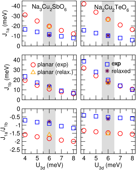
Figure 6: (Color online) Calculated exchange integrals $J_{1b}$ and $J_{1a}$, as well as frustration ratios $J_{1a}/J_{1b}\!=\!\alpha$ as a function of the Coulomb repulsion $U_{3d}$ for different structural models of the two compounds.

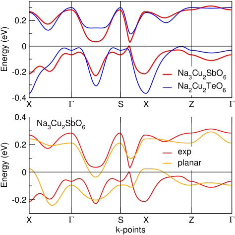
Figure 7: Top: LDA band structures showing the magnetically active antibonding dp$\sigma^{*}$ states for Na₃Cu₂SbO₆ and Na₂Cu₂TeO₆. Bottom: comparison of the LDA band structures calculated for different structural models of Na₃Cu₂SbO₆.

The direct comparison of the antibonding dp$\sigma^{*}$ bands for the experimentally observed crystal structures of Na₃Cu₂SbO₆ and Na₂Cu₂TeO₆ (Fig. 7, upper panel) reveals that these bands differ mainly by their width. In contrast, comparing the antibonding $dp\sigma^{*}$ bands of Na₃Cu₂SbO₆ within the experimental crystal structure (distorted plaquettes) with the fictitious crystal structure (planar plaquettes) reveals similar band widths, but substantially different dispersions (compare X-$\Gamma$ or X-Z in Fig. 7). The same trend is also observed for Na₂Cu₂TeO₆.

(i) To separate out the effect of the Sb$\leftrightarrow$Te substitution, we perform VCA calculations for the same structural model. In particular, a certain fraction $x$ of Sb atoms is replaced by Te, with a concomitant change in the Na content, in order to keep the charge balance. The band structures calculated for different Te concentrations exhibit similar dispersions and similar band width, evidencing the minor relevance of the pure substitutional effect for the magnetic exchange couplings.sup

To estimate the impact of the chain distortion and interatomic distances onto the magnetism in more detail, we evaluated the magnetic model also for two fictitious crystal structures of Na₃Cu₂SbO₆ and Na₂Cu₂TeO₆ (featuring planar dimer chains).sup The obtained hopping terms and exchange integrals are given in Tables 3 and 5. LSDA+$U$ calculations ($U_{3d}\!=\!6\pm 1$ eV) yield $J_{1a}$ = $-230\pm 50$ K and $J_{1b}\!=\!126\pm 35$ K for the fictitious Na₃Cu₂SbO₆ and $J_{1a}\!=\!-312\pm 80$ K and $J_{1b}\!=\!212\pm 45$ K for the fictitious Na₂Cu₂TeO₆, respectively. The dependence of the exchange integrals on the Coulomb repulsion $U_{3d}$ is depicted in Fig. 6. Analysis of the resulting exchange couplings suggests that the two structural parameters act differently: the distortion of the dimer-chains mainly influences the coupling strength of $J_{1a}$ and the coupling regime between the dimer-chains ($t_{ic}$ and $t_{il}$), whereas the interdimer exchange $J_{1b}$ is rather insensitive to this parameter (Table 5), since the respective superexchange path does not involve O(2) atoms that rule the distortion.

Table 5: DFT estimates for the magnetic exchange integrals in Na₃Cu₂SbO₆ and Na₂Cu₂TeO₆. The AFM part of the exchange integral $J^{\text{AFM}}_{1b}$ (in K) evaluated using the effective one-orbital model (with $U_{\text{eff}}$ = 4 eV) and total exchange integrals $J_{1b}$ and $J_{1a}$ (in K) from LSDA+$U$ total energy calculations (using $U_{3d}\!=\!6.0$ eV), for the experimental (exp), the LDA-relaxed (relaxed) and the fictitious (planar) crystal structures.

structure	$J_{1a}$	$J_{1b}$	($J^{\text{AFM}}_{1b}$)
Na3Cu2SbO6
exp	$-135$	150	(188)
relaxed	$-125$	162	(209)
planar (exp)	$-230$	126	(165)
planar (relax)	$-227$	142	(182)
Na2Cu2TeO6
exp	$-120$	232	(305)
relaxed	$-122$	197	(269)
planar (exp)	$-312$	212	(269)
planar (relax)	$-305$	200	(255)

(ii) Comparing the total exchange integrals for Na₃Cu₂SbO₆ for the experimental crystal structure with the planar system discloses an increase of the NN coupling $J_{1a}$ by nearly a factor of 2, whereas $J_{1b}$ is decreased by less than 20%. This observation is in line with the intuitive picture derived from geometrical considerations comparing the experimental distorted crystal structure to the fictitious system containing ideal planar chains (compare Fig. 1, lower panel). Locking the O atoms within the chain plane directly alters the exchange path of $J_{1a}$ along Cu-O-Cu, by a change of the Cu-O-Cu bridging angle and the orientation of the magnetically active orbitals. In contrast, the superexchange path of $J_{1b}$ (Cu-O-O-Cu) is altered only indirectly by changes of the crystal-field due to the distortion of the Sb/TeO₆ octahedra (compare Fig. 1, lower panel).

(iii) The modulation of interatomic distances influences $J_{1a}$ and $J_{1b}$ in a similar way. The crucial impact of the interatomic distances on $J_{1b}$ manifests itself in the coupling strength of the planar model structures for Na₃Cu₂SbO₆ and Na₂Cu₂TeO₆ (see Tab. 5) with the corresponding NNN Cu-Cu interdimer distance. The about 0.1 Å shorter NNN Cu-Cu distance in the fictitious planar Na₂Cu₂TeO₆ structure compared to the fictitious planar Na₃Cu₂SbO₆ increases the coupling strength by about 60%. However, comparing the experimental distorted crystal structure with the planar model structure of Na₂Cu₂TeO₆ the difference in the NNN Cu-Cu distance is only half as large (about 0.05 Å) as between the two planar structures and result in an about 1/4 smaller increase of $J_{1b}$. Thus, $J_{1b}$ follows a simple distance relation and scales according to $r^{2}$. The same relation holds for $J_{1a}$ (compare $J_{1a}$ for the two planar structures with the change of the NN Cu-Cu distance).

Based on the above considerations, we can conclude that the crucial parameter, determining the alteration ratio $\alpha\!=\!J_{1a}/J_{1b}$ for Na₃Cu₂SbO₆ and Na₂Cu₂TeO₆, is the distortion of the chains. Thus, a directed modification of the chain buckling by the appropriate substitution of ions should allow to tune the magnetism of these systems. Furthermore, the chain distortion also influences the interchain coupling regime. In the experimental structure the long-range exchanges mostly operate within the magnetic layers (in the $ab$-plane), whereas in the planar system the coupling between the layers is enhanced ($t_{ij}$’s in Table 3).

V Energy spectrum

As already mentioned, the FM-AFM and AFM-AFM solutions correspond to different magnetic GSs. In the former case, the GS is similar to the Haldane chain and features sizable string order parameter $O_{\text{s}}\!=\!0.36$, indicative of a topological order, while in the latter case the string order is suppressed ($O_{\text{s}}\!=\!0.16$).Watanabe and Yokoyama (1999) It is thus tempting to find an observable quantity that would be substantially different in the two phases. Theoretical studies of the $S\!=\!1/2$ AHC model suggest that this requirement is fulfilled for the momentum position of the spin gap. Indeed, the $Q\!=\!0$ gap is characteristic for AFM-AFM chains, except for the narrow parameter range $\alpha\!=\!0.79-1.00$, where the gap shifts to small finite $Q\leq 0.02/\pi$.Johnston et al. (2000) In contrast, the spin gap in the FM-AFM chains is located at $Q\!=\!\pi$.Hida (1994) Therefore, by measuring momentum resolved excitation spectra, the sign of $J_{1a}$ can be reliably determined.

To resolve the ambiguity between the FM-AFM and AFM-AFM cases ultimately, we calculate the low-energy excitations for $\alpha\!=\!-1.25$ as well as $\alpha\!=\!0.4$ using Lanczos diagonalization of the respective Heisenberg Hamiltonian. The resulting $E(Q)$ dependence is plotted in Fig. 8. Although the two solutions yield similar estimates for the spin gap, its $Q$-position is very different: $Q\!=\!\pi$ and $Q\!=\!0$, for the FM-AFM and AFM-AFM solution, respectively. Another distinct feature of the excitation spectra is the well-separated branch of lowest-energy excitations (Fig. 8). For the FM-AFM solution, this branch resembles the behavior of $\cos(Q)$, while the AFM-AFM solution yields a $\sin(Q)$-like behavior.

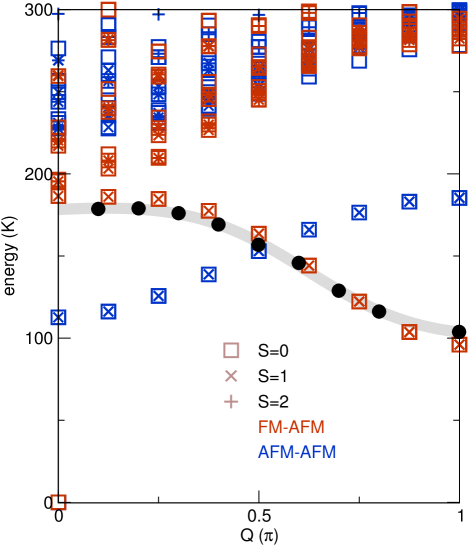
Figure 8: (Color online) Low-energy excitation spectra for the alternating Heisenberg chains of $N\!=\!32$ spins, corresponding to the QMC solutions (FM-AFM and AFM-AFM) from Table 2. Note the difference in the behavior of the low-lying branch for the two solutions. Experimental data from Ref. Miura et al., 2008 are shown with filled circles (the gray line is guide to the eye).

To compare with the experimental dispersion from Ref. Miura et al., 2008, we scale the two spectra using the values of the exchange couplings from our QMC fits to the magnetic susceptibility (Table 2, last row). This way, we find that the FM-AFM solution agrees very well with the experimental data (Fig. 8), while the AFM-AFM solution can be safely ruled out.

Fig. 8 also provides an answer to an intriguing question, why both $\alpha\!=\!-1.25$ and $\alpha\!=\!0.4$ provide good fits to the susceptibility data. At finite temperature, magnetic susceptibility reflects the thermal-averaged magnetic spectrum integrated over the whole momentum space. Thus, at low temperatures, $\chi(T)$ is largely affected by the value of the spin gap, but is insensitive to its $Q$ position. Since the values of the spin gap for the two solutions are very similar (around 100 K), the similarity of the low-temperature $\chi(T)$ is also not surprising. Moreover, the shape of the low-energy branch is similar (but reflected around $Q\!=\!\pi/2$), thus the $Q$-integrated spectrum is nearly the same in both cases. Only at elevated temperatures, the contribution of high-lying states gives rise to the difference in $\chi(T)$. This is in excellent agreement with the enhanced deviation of the AFM-AFM solution at high temperatures (Fig. 2, inset).

VI Summary

Since the first report on the magnetism of the low-dimensional $S$ = 1/2 systems Na₃Cu₂SbO₆ and Na₂Cu₂TeO₆, their spin models were controversially debated in the literature. The main conundrum was the sign of the exchange coupling $J_{\text{1a}}$ operating within the structural Cu₂O₆ dimers. To resolve the conflicting reports, we applied a series of different computational methods, including density functional theory (DFT) band structure, virtual crystal approximation, DFT+$U$, and hybrid functional calculations, as well as high-temperature series expansions, quantum Monte Carlo simulations, and exact diagonalization.

Our calculations evidence that the magnetism of both compounds can be described by the alternating Heisenberg chain model with two relevant couplings: ferromagnetic $J_{\text{1a}}$ within the structural dimers, and antiferromagnetic $J_{\text{1b}}$ between the dimers. The alternation parameter $\alpha\!=\!J_{\text{1a}}/J_{\text{1b}}$ amounts to about $-1.25$ and $-0.55$ in Na₃Cu₂SbO₆ and Na₂Cu₂TeO₆, respectively. This parameter regime corresponds to the Haldane phase, characterized by the gapped excitation spectrum and a topological string order.

Using extensive calculations for different structural models, we find that the physically relevant ratio $\alpha\!=\!J_{1a}/J_{1b}$ is primarily ruled by the distortion of the structural chains, while the Sb$\leftrightarrow$Te substitution and the change in the Cu–Cu distance play a minor role. A comparison of the simulated dispersion $E(Q)$ with the experimental inelastic neutron scattering data (Ref. Miura et al., 2008) yields an unequivocal evidence for the FM nature of $J_{\text{1a}}$ in Na₃Cu₂SbO₆. These spectra facilitate the understanding of the similarity between the magnetic susceptibility curves for mutually exclusive solutions that involve ferromagnetic and antiferromagnetic $J_{\text{1a}}$.

It is important to note that the problem of ambiguous solutions appears in the empirical modeling, only. In contrast, the microscopic modeling based on DFT calculations readily yields a quasi-one-dimensional model with the ferromagnetic $J_{\text{1a}}$. This clearly indicates that present-day DFT calculations are a reliable tool to disclose even rather complicated cases and deliver a reliable microscopic magnetic model. Since the correctness of the magnetic model is of crucial importance for its refinement and extension, DFT calculations should be an indispensable ingredient of real-material studies.

Table 6: Crystal structures for Na₃Cu₂SbO₆ used in the DFT study. The experimental structure is adopted from Ref. Smirnova et al., 2005. The fictitious planar structures deviate from the experimental ones only by the coordinate of the O$(2)$ site. The relaxed structures were optimized with respect to the LDA total energy.

Na3Cu2SbO6– experimental structures
	exp.				relaxed
	$x/a$	$y/b$	$z/c$		$x/a$	$y/b$	$z/c$
Cu	0	0.6667	0		0	0.6667	0
Sb	0	0	0		0	0	0
O(1)	0.2931	0.3340	0.7750		-0.1987	-0.1667	-0.2234
O(2)	0.2404	0.5	0.1774		-0.2619	0	0.1734
Na(1)	0	0.5	0.5		0	-0.5	-0.5
Na(2)	0.5	0.3280	0.5		0	-0.1732	-0.5
Na3Cu2SbO6– fictitious structures
	planar exp.				planar relaxed
O(2)	0.2931	0.5	0.7750		-0.1987	0.5	-0.2234

Table 7: Crystal structures for Na₂Cu₂TeO₆ used in the DFT study. The experimental structure is adopted from Ref.  Xu et al., 2005. The fictitious planar structures deviate from the experimental ones only by the coordinate of the O$(2)$ site. The relaxed structures were optimized with respect to the LDA total energy.

Na2Cu2TeO6– experimental structures
	exp.				relaxed
	$x/a$	$y/b$	$z/c$		$x/a$	$y/b$	$z/c$
Cu	0	0.66475	0		0	-0.3353	0
Te	0	0	0		0	0	0
O(1)	0.1936	0.1632	0.2121		0.1906	0.1682	0.2156
O(2)	0.7574	0	0.1640		-0.2519	0	0.1648
Na	0	0.1839	0.5		0	0.1849	-0.5
Na2Cu2TeO6– fictitious structures
	planar exp.				planar relaxed
O(2)	0.1936	0.5	0.2121		0.1906	0.5	0.2156

Table 8: Transfer integrals $t_{ij}$ (in meV) evaluated by fitting the LSDA band structures for the different structural models: experimental (exp), LSDA-relaxed (relaxed) and fictitious planar structures originating from the experimental ones by shifting O(2) (planar exp and planar relaxed). For the notation of $t_{ij}$, see Fig. 5 in the manuscript. (”$-$” $<1$ meV)

Na3Cu2SbO6
$t_{i}$/meV	$t_{1a}$	$t_{1b}$	$t_{2}$	$t^{ic}_{1a}$	$t^{ic}_{1b}$	$t_{1a}^{il}$	$t_{1b}^{il}$	$t_{0}^{d}$	$t_{1}^{d}$	$t_{0}^{a}$
exp	60.6	127	18.2	$-$27.8	17.0	5.8	$-$6.6	21.8	$-$4.6	17.4
relaxed	68.2	134	18.1	$-$32.3	20.6	6.4	$-$7.2	20.9	$-$3.8	19.2
planar exp	45.3	119	22.4	$-$7.8	9.4	14.1	$-$18.8	30.1	$-$13.2	$-$
planar relaxed	55.6	125	23.8	$-$9.2	10.7	17.3	$-$21.7	29.2	$-$19.9	$-$
Na2Cu2TeO6
$t_{i}$/meV	$t_{1a}$	$t_{1b}$	$t_{2}$	$t^{ic}_{1a}$	$t^{ic}_{1b}$	$t_{1a}^{il}$	$t_{1b}^{il}$	$t_{0}^{d}$	$t_{1}^{d}$	$t_{0}^{a}$
exp	15.6	162	16.4	$-$38.5	24.7	2.8	$-$ 2.5	13.7	$-$	25.5
relaxed	42.5	152	17.3	$-$42.4	26.3	3.4	$-$3.9	14.5	$-$	23.1
planar exp.	27.3	152	29.3	$-$12.6	12.4	14.1	$-$16.0	25.6	$-$11.8	1.3
planar relaxed	45.2	148	30.0	$-$12.8	12.7	16.0	$-$18.6	26.0	$-$10.7	$-$

Table 9: Exchange integrals derived from the LSDA+$U$ total energy calculation for different structural models ($U_{3d}$ = $6.0$ eV). For comparison the AFM parts of exchange integrals estimated from the effective one-orbital approach (tight-binding model $\rightarrow$ Hubbard model $\rightarrow$ Heisenberg model, $U_{\text{eff}}$ = 4 eV) are given in brackets. The ”$-$” sign means that the respective coupling was not evaluated.

Na3Cu2SbO6
$J_{i}$/meV	$J_{1a}$	($J_{1a}^{AFM}$)	$J_{1b}$	($J_{1b}^{AFM}$)	$J_{2}$+$J_{1b}^{ic}$+$J_{1b}^{il}$	$J^{ic}_{1a}$+$J^{ic}_{1b}$	$J^{d}_{0}$+$J^{d}_{1}$
exp	-11.6		12.9		-0.01	0.8	0.4
		(3.7)		(16.1)
relaxed	-10.7		13.9		0.3	0.7	$-$
		(4.7)		(18.0)
planar exp	-19.7		10.8		0.9	0.2	1.2
		(2.1)		(14.2)
planar relaxed	-19.5		12.2		1.0	0.2	$-$
		(3.1)		(15.7)
Na2Cu2TeO6
$J_{i}$/meV	$J_{1a}$	($J_{1a}^{AFM}$)	$J_{1b}$	($J_{1b}^{AFM}$)	$J_{2}$+$J_{1b}^{ic}$+$J_{1b}^{il}$	$J^{ic}_{1a}$+$J^{ic}_{1b}$	$J^{d}_{0}$+$J^{d}_{1}$
exp	-10.3		19.9		0.1	1.0	0.1
		(0.2)		(26.2)
relaxed	-10.5		16.9		0.2	1.0	$-$
		(1.8)		(23.1)
planar exp.	-26.8		18.2		1.2	0.5	0.8
		(0.8)		(23.1)
planar relaxed	-26.2		17.2		1.5	0.6	$-$
		(2.0)		(21.9)

Table 10: Comparison of representative interatomic distances (in Å) and bond angles (in deg.) for the different structures. $d_{\text{NN}}$ and $d_{\text{NNN}}$ correspond to the nearest-neighbor and next-nearest-neighbor Cu–Cu distances. Cu–O–Cu is the bond angle within the structural dimer. O–O is the shortest distance between O atoms in the neighboring structural dimers. Cu–O are the distances within the CuO₄ plaquette. $\delta$O is the distance (in Å) between the O(2) atom in the experimental structure and the respective atom in the ideal planar chain geometry.

structure	$d_{\text{NN}}$	$d_{\text{NNN}}$	Cu–O–Cu	O–O	Cu–O	$\delta$O
Na3Cu2SbO6
exp	2.96	5.91	95.27	2.94	2.021/2.000	0.39
planar exp	2.96	5.91	94.22	2.94	2.021/2.017	0
relaxed	2.96	5.91	96.03	2.96	1.998/1.988	0.43
planar relaxed	2.96	5.91	95.39	2.96	1.998/1.998	0
Na2Cu2TeO6
exp	2.86	5.82	91.27	2.83	1.978/1.999	0.55
planar exp	2.86	5.82	95.48	2.83	1.978/1.931	0
relaxed	2.86	5.82	92.91	2.92	1.950/1.972	0.53
planar relaxed	2.86	5.82	95.24	2.92	1.950/1.935	0

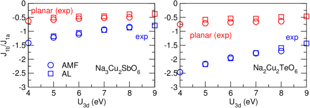
Figure 9: Dependence of exchange integrals on the double-counting correction: the around-mean-field (AMF) and the atomic limit (AL). For the LSDA+$U$ calculations we adopted the experimental crystal structure (exp) and the structure with planar chains (planar exp).

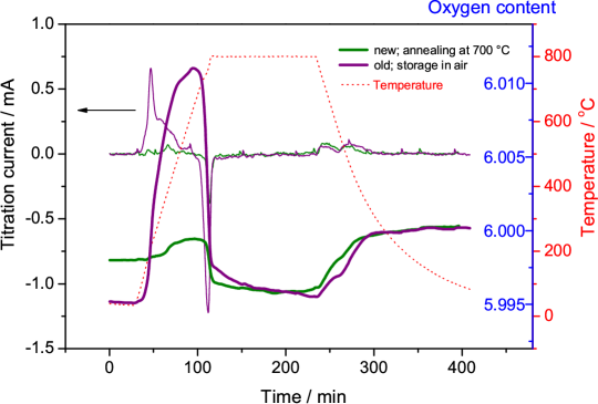
Figure 10: Oxygen content determined by coulometric titration of a freshly annealed sample (green curve) and a sample stored at room temperature and in air (violet curve). Note the difference between the initial oxygen content in the two samples.

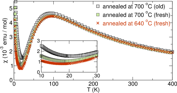
Figure 11: Dependence of the magnetic susceptibility on the annealing temperature and sample history (quality) due to changes in the O occupation. External magnetic field is 0.04 T. Note the difference between the 700 ^∘C samples stored in air (“old”) and measured right after annealing (“fresh”). In the paper, we used $\chi(T)$ data for fresh samples annealed at 640 ^∘C, i.e., the samples featuring the smallest Curie-law-type impurities and/or defects (inset).

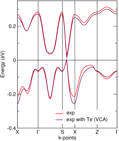
Figure 12: Comparison of the antibonding $dp\sigma$ band using LDA for the experimental crystal structure of Na₃Cu₂SbO₆ and a model compound where Sb is substituted by Te (with an concomitant change in the Na content) within the same crystal structure using VCA. The obtained bands show nearly the same band width and shape pointing to minor relevance of pure substitutional effects.

References

- Lee (2008) P. A. Lee, Rep. Prog. Phys. 71, 012501 (2008), arXiv:0708.2115 .
- Balents (2010) L. Balents, Nature (London) 464, 199 (2010).
- Helton et al. (2007) J. S. Helton, K. Matan, M. P. Shores, E. A. Nytko, B. M. Bartlett, Y. Yoshida, Y. Takano, A. Suslov, Y. Qiu, J.-H. Chung, D. G. Nocera, and Y. S. Lee, Phys. Rev. Lett. 98, 107204 (2007), cond-mat/0610539 .
- Nakatsuji et al. (2012) S. Nakatsuji, K. Kuga, K. Kimura, R. Satake, N. Katayama, E. Nishibori, H. Sawa, R. Ishii, M. Hagiwara, F. Bridges, T. U. Ito, W. Higemoto, Y. Karaki, M. Halim, A. A. Nugroho, J. A. Rodriguez-Rivera, M. A. Green, and C. Broholm, Science 336, 559 (2012).
- Isobe and Ueda (1996) M. Isobe and Y. Ueda, J. Phys. Soc. Jpn. 65, 3142 (1996).
- Valentí and Saha-Dasgupta (2002) R. Valentí and T. Saha-Dasgupta, Phys. Rev. B 65, 144445 (2002), cond-mat/0110311 .
- Saúl and Radtke (2011) A. Saúl and G. Radtke, Phys. Rev. Lett. 106, 177203 (2011).
- Deisenhofer et al. (2006) J. Deisenhofer, R. M. Eremina, A. Pimenov, T. Gavrilova, H. Berger, M. Johnsson, P. Lemmens, H.-A. Krug von Nidda, A. Loidl, K.-S. Lee, and M.-H. Whangbo, Phys. Rev. B 74, 174421 (2006), cond-mat/0610458 .
- Das et al. (2008) H. Das, T. Saha-Dasgupta, C. Gros, and R. Valentí, Phys. Rev. B 77, 224437 (2008), cond-mat/0703675 .
- Ushakov and Streltsov (2009) A. V. Ushakov and S. V. Streltsov, J. Phys.: Condens. Matter 21, 305501 (2009).
- Sasago et al. (1995) Y. Sasago, M. Hase, K. Uchinokura, M. Tokunaga, and N. Miura, Phys. Rev. B 52, 3533 (1995).
- Valentí et al. (2002) R. Valentí, T. Saha-Dasgupta, and C. Gros, Phys. Rev. B 66, 054426 (2002), cond-mat/0202310 .
- Schmitt et al. (2010) M. Schmitt, A. A. Gippius, K. S. Okhotnikov, W. Schnelle, K. Koch, O. Janson, W. Liu, Y.-H. Huang, Y. Skourski, F. Weickert, M. Baenitz, and H. Rosner, Phys. Rev. B 81, 104416 (2010).
- Mazurenko et al. (2014) V. V. Mazurenko, M. V. Valentyuk, R. Stern, and A. A. Tsirlin, (2014), arXiv:1309.6762 .
- Jaime et al. (2004) M. Jaime, V. F. Correa, N. Harrison, C. D. Batista, N. Kawashima, Y. Kazuma, G. A. Jorge, R. Stern, I. Heinmaa, S. A. Zvyagin, Y. Sasago, and K. Uchinokura, Phys. Rev. Lett. 93, 087203 (2004), cond-mat/0404324 .
- Sebastian et al. (2006) S. E. Sebastian, N. Harrison, C. D. Batista, L. Balicas, M. Jaime, P. A. Sharma, N. Kawashima, and I. R. Fisher, Nature (London) 441, 617 (2006), cond-mat/0606042 .
- Krämer et al. (2007) S. Krämer, R. Stern, H. M., C. Berthier, T. Kimura, and I. R. Fisher, Phys. Rev. B 76, 100406 (2007), arXiv:0704.0888 .
- Takigawa et al. (2010) M. Takigawa, T. Waki, M. Horvatić, and C. Berthier, J. Phys. Soc. Jpn. 79, 011005 (2010).
- Goodenough (1955) J. B. Goodenough, Phys. Rev. 100, 564 (1955).
- Kanamori (1959) J. Kanamori, J. Phys. Chem. Solids 10, 87 (1959).
- Pickett (1989) W. E. Pickett, Rev. Mod. Phys. 61, 433 (1989).
- Miura et al. (2006) Y. Miura, R. Hirai, Y. Kobayashi, and M. Sato, J. Phys. Soc. Jpn. 75, 084707 (2006).
- Derakhshan et al. (2007) S. Derakhshan, H. L. Cuthbert, J. E. Greedan, B. Rahaman, and T. Saha-Dasgupta, Phys. Rev. B 76, 104403 (2007).
- Yamanaka et al. (1993) M. Yamanaka, Y. Hatsugai, and M. Kohmoto, Phys. Rev. B 48, 9555 (1993).
- Koo and Whangbo (2008) H.-J. Koo and M.-H. Whangbo, Inorg. Chem. 47, 128 (2008).
- Miura et al. (2008) Y. Miura, Y. Yasui, T. Moyoshi, M. Sato, and K. Kakurai, J. Phys. Soc. Jpn. 77, 104709 (2008).
- Xu et al. (2005) J. Xu, A. Assoud, N. Soheilnia, S. Derakhshan, H. L. Cuthbert, J. E. Greedan, M. H. Whangbo, and H. Kleinke, Inorg. Chem. 44, 5042 (2005).
- Smirnova et al. (2005) O. A. Smirnova, V. B. Nalbandyan, A. A. Petrenko, and M. Avdeev, J. Solid State Chem. 178, 1165 (2005).
- (29) See Supplementary information for the crystal structures, full set of transfer integrals, depdence of the exchange integrals on the structural model, temperature dependence of magnetic susceptibility as a function of oxygen deficiency, as well as auxilary DOS and band structure plots.
- Koepernik and Eschrig (1999) K. Koepernik and H. Eschrig, Phys. Rev. B 59, 1743 (1999).
- Perdew and Wang (1992) J. P. Perdew and Y. Wang, Phys. Rev. B 45, 13244 (1992).
- Kasinathan et al. (2012) D. Kasinathan, M. Wagner, K. Koepernik, R. Cardoso-Gil, Y. Grin, and H. Rosner, Phys. Rev. B 85, 035207 (2012).
- Heyd et al. (2003) J. Heyd, G. E. Scuseria, and M. Ernzerhof, J. Chem. Phys. 118, 8207 (2003).
- Heyd et al. (2006) J. Heyd, G. E. Scuseria, and M. Ernzerhof, J. Chem. Phys. 124, 219906 (2006).
- Kresse and Furthmüller (1996a) G. Kresse and J. Furthmüller, Phys. Rev. B 54, 11169 (1996a).
- Kresse and Furthmüller (1996b) G. Kresse and J. Furthmüller, Comput. Mater. Sci. 6, 15 (1996b).
- Johnston et al. (2000) D. C. Johnston, R. K. Kremer, M. Troyer, X. Wang, A. Klümper, S. L. Bud’ko, A. F. Panchula, and P. C. Canfield, Phys. Rev. B 61, 9558 (2000), arXiv:cond-mat/0003271 .
- Borras-Almenar et al. (1994) J. J. Borras-Almenar, E. Coronado, J. Curely, R. Georges, and J. C. Gianduzzo, Inorg. Chem. 33, 5171 (1994).
- Todo and Kato (2001) S. Todo and K. Kato, Phys. Rev. Lett. 87, 047203 (2001), cond-mat/9911047 .
- Albuquerque et al. (2007) A. Albuquerque, F. Alet, P. Corboz, P. Dayal, A. Feiguin, S. Fuchs, L. Gamper, E. Gull, S. Gürtler, A. Honecker, R. Igarashi, M. Körner, A. Kozhevnikov, A. Läuchli, S. R. Manmana, M. Matsumoto, I. P. McCulloch, F. Michel, R. M. Noack, G. Pawlowski, L. Pollet, T. Pruschke, U. Schollwöck, S. Todo, S. Trebst, M. Troyer, P. Werner, and S. Wessel, J. Magn. Magn. Mater. 310, 1187 (2007), arXiv:0801.1765 .
- (41) J. Schulenburg, http://www-e.uni-magdeburg.de/jschulen/spin.
- Belik et al. (2004) A. A. Belik, M. Azuma, and M. Takano, J. Solid State Chem. 177, 883 (2004).
- Volkova et al. (2010) O. Volkova, I. Morozov, V. Shutov, E. Lapsheva, P. Sindzingre, O. Cépas, M. Yehia, V. Kataev, R. Klingeler, B. Büchner, and A. Vasiliev, Phys. Rev. B 82, 054413 (2010), arXiv:1004.0444 .
- Hall et al. (1981) J. W. Hall, W. E. Marsh, R. R. Weller, and W. E. Hatfield, Inorg. Chem. 20, 1033 (1981).
- Schmitt et al. (2009) M. Schmitt, J. Málek, S.-L. Drechsler, and H. Rosner, Phys. Rev. B 80, 205111 (2009), arXiv:0911.0307 .
- Wolter et al. (2012) A. U. B. Wolter, F. Lipps, M. Schäpers, S.-L. Drechsler, S. Nishimoto, R. Vogel, V. Kataev, B. Büchner, H. Rosner, M. Schmitt, M. Uhlarz, Y. Skourski, J. Wosnitza, S. Süllow, and K. C. Rule, Phys. Rev. B 85, 014407 (2012), arXiv:1110.4729 .
- Fuchs et al. (2007) F. Fuchs, J. Furthmüller, F. Bechstedt, M. Shishkin, and G. Kresse, Phys. Rev. B 76, 115109 (2007), cond-mat/0604447 .
- Andersen and Saha-Dasgupta (2000) O. K. Andersen and T. Saha-Dasgupta, Phys. Rev. B 62, R16219 (2000).
- Andersen and Jepsen (1984) O. K. Andersen and O. Jepsen, Phys. Rev. Lett. 53, 2571 (1984).
- Rosner et al. (2009) H. Rosner, M. Schmitt, D. Kasinathan, A. Ormeci, J. Richter, S.-L. Drechsler, and M. D. Johannes, Phys. Rev. B 79, 127101 (2009).
- Ylvisaker et al. (2009) E. R. Ylvisaker, W. E. Pickett, and K. Koepernik, Phys. Rev. B 79, 035103 (2009), arXiv:0808.1706 .
- Watanabe and Yokoyama (1999) S. Watanabe and H. Yokoyama, J. Phys. Soc. Jpn. 68, 2073 (1999), cond-mat/9902311 .
- Hida (1994) K. Hida, J. Phys. Soc. Jpn. 63, 2514 (1994).
Supplementary information for

References

- Smirnova et al. (2005) O. A. Smirnova, V. B. Nalbandyan, A. A. Petrenko, and M. Avdeev, J. Solid State Chem. 178, 1165 (2005).
- Xu et al. (2005) J. Xu, A. Assoud, N. Soheilnia, S. Derakhshan, H. L. Cuthbert, J. E. Greedan, M. H. Whangbo, and H. Kleinke, Inorg. Chem. 44, 5042 (2005).