Abstract

The periodic $3D$ Navier-Stokes equations are analyzed in terms of dimensionless, scaled, $L^{2m}$-norms of vorticity $D_{m}$ ($1\leq m<\infty$). The first in this hierarchy, $D_{1}$, is the global enstrophy. Three regimes naturally occur in the $D_{1}-D_{m}$ plane. Solutions in the first regime, which lie between two concave curves, are shown to be regular, owing to strong nonlinear depletion. Moreover, numerical experiments have suggested, so far, that all dynamics lie in this heavily depleted regime [1] ; new numerical evidence for this is presented. Estimates for the dimension of a global attractor and a corresponding inertial range are given for this regime. However, two more regimes can theoretically exist. In the second, which lies between the upper concave curve and a line, the depletion is insufficient to regularize solutions, so no more than Leray’s weak solutions exist. In the third, which lies above this line, solutions are regular, but correspond to extreme initial conditions. The paper ends with a discussion on the possibility of transition between these regimes.

1 Introduction

Kolmogorov’s phenomenological statistical theory of turbulence, based on a set of axioms, displays certain well-known characteristics, such as a $k^{-5/3}$ spectrum in an inertial range with a wavenumber cut-off at $L^{-1}Re^{3/4}$, together with a dissipation range beyond this [2-5]. In contrast, from the perspective of Navier-Stokes analysis, much remains open in the three-dimensional case [6-19]. A proof of the existence and uniqueness of solutions is missing so the existence of a global attractor remains an open question [10-13]. Moreover, characteristics of an energy spectrum, such as its steepness and wavenumber cut-off, are hard to extract from a time-evolving PDE. An interesting question is whether numerical experiments on the Navier-Stokes equations can inform the analysis by suggesting a new and different way of looking at Navier-Stokes turbulence? In the early days of Navier-Stokes simulations [20-25] less resolution was available but, in recent years, several very large simulations (up to a maximum of $4096^{3}$) have been performed [26-32]. The data from two of these, together with additional computations, are used in an attempt to understand the behaviour of the solutions from a range of initial conditions.

The variables that will be used in this paper are defined in terms of the Navier-Stokes vorticity field $\mbox{\boldmath$\omega$}=\mbox{curl}\,\mbox{\boldmath$u$}$ in the following manner [1, 33-36] :

$$\Omega_{m}(t)=\left(L^{-3}\int_{\mathcal{V}}|\mbox{\boldmath$\omega$}|^{2m}dV\right)^{1/2m}\,;\qquad D_{m}=\left(\varpi_{0}^{-1}\Omega_{m}\right)^{\alpha_{m}}\,;\qquad\alpha_{m}=\frac{2m}{4m-3}\,,$$ (1.1)

where $\varpi_{0}=\nu L^{-2}$ is the frequency on the periodic box $[0,\,L]^{3}$. Note that $D_{1}=\left(\varpi_{0}^{-1}\Omega_{1}\right)^{2}$ is proportional to the $H_{1}$-norm of the velocity field. A recent set of numerical experiments, using a variety of initial conditions, each with periodic boundary conditions [1], has suggested that the $D_{m}$ are ordered on a descending scale such that $D_{m+1}<D_{m}$ for $m\geq 1$. In itself this is not surprising : while Hölder’s inequality necessarily enforces the $\Omega_{m}$ to be ordered on an ascending scale such that $\Omega_{m}\leq\Omega_{m+1}$, the decreasing nature of the $\alpha_{m}$ means that if the $\Omega_{m}$ are bunched sufficiently close, the ordering of the $D_{m}$ could easily be the reverse of the $\Omega_{m}$, as indeed is observed numerically. What is more surprising is the observed strong separation on a logarithmic scale in the descending sequence of the $D_{m}$, in particular from $D_{1}$. This separation is observed to be of the form (see §2)

$$D_{1}^{\alpha_{m}/2}\leq D_{m}\leq D_{1}^{A_{m}}\,,\qquad\qquad m\geq 2\,,$$ (1.2)

where ${\scriptstyle\frac{1}{2}}\alpha_{m}<A_{m}(t)<{\scriptstyle\frac{1}{2}}$ : the lower bound arises from $\Omega_{1}\leq\Omega_{m}$ expressed in the $D_{m}$-notation.

The main intention of this paper is to investigate how the numerically observed depletion in (1.2) severely reduces the strength of the vortex stretching, thereby opening a window through which we can examine its effect on the regularity problem. To illustrate how this comes about, let us summarize the results which standard methods (Hölder and Sobolev inequalities) yield when attempting to estimate the rate of enstrophy production $\dot{D}_{1}$. The result in the unforced case is

$${\scriptstyle\frac{1}{2}}\dot{D}_{1}\leq\varpi_{0}\left(-D_{1}^{2}/4E+c\,D_{1}^{3}\right)\,,$$ (1.3)

where the dimensionless, bounded energy is $E=\nu^{-2}L^{-1}\int_{\mathcal{V}}|\mbox{\boldmath$u$}|^{2}dV$. This result has been known for a generation [10, 11, 12, 13] and is derived for the reader in §2. As it stands, (1.3) allows no control over $D_{1}$ beyond short times for arbitrarily large initial data or for long times from very small initial data. Moreover, dimensional scaling arguments suggest that no improvement on the $D_{1}^{3}$-term can be obtained when standard methods are used. However, §2 shows that a re-working of this term by the insertion of the nonlinear depletion

$$D_{m}\leq D_{1}^{A_{m,\lambda}}\,,\qquad\mbox{where}\qquad A_{m,\lambda}=\max_{t}A_{m}(t)$$ (1.4)

results in the $D_{1}^{3}$-term being replaced by one proportional to $D_{1}^{\xi_{m,\lambda}}$ (see (3.12)) where :

$$\xi_{m,\lambda}=\frac{\chi_{m,\lambda}+2m-3}{2(m-1)}\,,\qquad\mbox{with}\qquad\chi_{m,\lambda}=A_{m,\lambda}(4m-3)\,.$$ (1.5)

The parameter $\lambda$, lying in the range $1\leq\lambda\leq 4$, appears through a scaling argument in §2.2 which suggests that $A_{m,\lambda}$ and $\chi_{m,\lambda}$ take the form

$$A_{m,\lambda}=\frac{m\lambda+1-\lambda}{4m-3}\quad\mbox{and}\quad\chi_{m,\lambda}=m\lambda+1-\lambda\,.$$ (1.6)

Note that when $\lambda=4$, then $A_{m,4}=1$. The value of $\lambda$ chosen in the above range depends on the initial conditions of a given numerical simulation. Equations (1.5) and (1.6) yield

$$\xi_{m,\lambda}=1+{\scriptstyle\frac{1}{2}}\lambda$$ (1.7)

which is explicitly independent of $m$. To gain control over $D_{1}$, for long times and large initial data, it is thus necessary to restrict $\xi_{m,\lambda}$ to $\xi_{m,\lambda}<2$ and $\lambda$ to the range $1\leq\lambda<2$ : see Fig. 1. It appears that the numerical data in [1] can be fitted to (1.6) with $\lambda$ sitting well within this range : $\lambda_{\rm min}$ is chosen as the minimum value of $\lambda$ for any given numerical fit. In §2.1 we suggest that the range $1.15\leq\lambda_{\rm min}\leq 1.5$ is appropriate for a range of initial conditions.

Figure 1: A cartoon of the three regimes in the $D_{1}-D_{m}$ plane represented by the inequalities in (1) at some value of $m>1$, with $A_{m,\lambda}$ defined in (1.4). Two solid concave curves bound regime I : the lower curve derives from Hölder’s inequality and corresponds to $\lambda=1$, whereas the upper curve is the upper limit of the regular regime (see §3) which corresponds to $\lambda=2$. The dotted curves approximately denote the region where the computations of §2.1 lie for various values of $\lambda$ in the range $1.15\leq\lambda\leq 1.5$. The line $D_{m}=C_{m}D_{1}$ separates regimes II and III.

While (1.4) is designated as regime I it is nevertheless theoretically possible that there exist other regimes beyond this (see Fig 1). The following regimes are defined and analyzed in §3 and §4 :

$$D_{1}^{\alpha_{m}/2} \leq D_{m}\leq D_{1}^{A_{m,\lambda}}\,,\qquad\qquad~{}~{}\mbox{(regime~{}I)}\,;$$

$$D_{1}^{A_{m,\lambda}} < D_{m}\leq C_{m}D_{1}\,,~{}~{}\qquad\qquad\mbox{(regime~{}II)}\,;$$ (1.8)

$$C_{m}D_{1} < D_{m}\,,\qquad\qquad\qquad\qquad~{}~{}\mbox{(regime~{}III)}\,,$$

with regime I corresponding to the range $1\leq\lambda\leq 2$. The constant $C_{m}$ is determined in §4, where it is shown that regime II leads to no improvement in the $D_{1}^{3}$ estimate. Solutions are actually regular in regime III, but it is an open question whether this regime is physical. Fig. 1 is a cartoon of the regimes in (1).

Remarkably, the two respective values of the exponents $\xi_{m,\lambda}=1+{\scriptstyle\frac{1}{2}}\lambda$ and $\xi_{m,4}=3~{}(\lambda=4)$ in regimes I and II, are close to those found in a paper by Lu and Doering [37], who used a numerical calculus of variations argument to find the value(s) of the exponent $\xi_{m,\lambda}$ when the rate of enstrophy production is maximized subject to the constraint $\mbox{div}\,\mbox{\boldmath$u$}=0$. They found that two branches existed, the lower being $D_{1}^{1.78}$ and the uppermost $D_{1}^{2.997}$. Later, Schumacher, Eckhardt and Doering [38] suggested that 7/4 and 3 were the likely values of these two exponents ; the exponent $\xi_{m,\lambda}=7/4$ corresponds to $\lambda=1.5$ which lies at the upper end of our observed range $1.15\leq\lambda\leq 1.5$.

Boundedness from above of $D_{1}$ establishes existence and uniqueness and is the missing ingredient in the search for the existence of a global attractor $\mathcal{A}$ [10-13], albeit limited to regime I. In §3.2 it is shown that estimates for the Lyapunov dimension of $\mathcal{A}$ are found to be (Proposition 3)

$$d_{L}(\mathcal{A})\leq c_{m}Re^{\frac{3(6-\lambda)}{5(2-\lambda)}}~{}~{}~{}\mbox{or}~{}~{}~{}c_{m}Gr^{\frac{3(4-\lambda)}{5(2-\lambda)}}\,,$$ (1.9)

where $Re$ and $Gr$ are respectively the Reynolds and Grashof numbers defined in §2. §5 shows that there is a corresponding energy spectrum in an inertial range for which $\mathcal{E}(k)\sim k^{-q_{m,\lambda}}$ where $q_{m,\lambda}=3-4/3\lambda$, with a cut-off at $L^{-1}Re^{3\lambda/4}$. The lower concave curve in Fig. 1 corresponds to $\lambda=1$ for which $q_{m,1}=5/3$ with a cut-off at $L^{-1}Re^{3/4}$. Regime I corresponds to $5/3\leq q_{m,\lambda}<7/3$.

If these properties of regime I turn out to be typical of Navier-Stokes flows in periodic domains, then the existence and uniqueness results derived here are consistent with the observation that both numerical solutions [20-32] and experimental data [39, 40], while providing evidence of strong intermittency, have shown none of the violent super-exponential or singular growth observed in the 3D Euler equations [41, 42], nor have they shown any positive evidence of a lack of uniqueness. A related question is why a regime with such heavy depletion is favoured? Moreover, what vortical structures would correspond to it? Formally, using Sobolev and Hölder inequalities in $d$ dimensions ($1\leq d\leq 3$) to estimate the vortex-stretching term, as in (1.3), results in $\xi_{m,\lambda}=(6-d)/(4-d)$, which takes the expected value $\xi_{m,4}=3$ when $d=3$. The value of $d$ corresponding to $\xi_{m,\lambda}=1+{\scriptstyle\frac{1}{2}}\lambda$ is $d_{\lambda}=4(\lambda-1)/\lambda$ which takes values from $d_{1.15}\approx 0.52$ to $d_{1.5}=4/3$. This suggests that the dominant structures which give rise to the depletion observed in regime I could be the pasta-mix of tubes on which both vorticity and strain have long been numerically observed to accumulate [39, 43] but also suggests that some vortical structures may lie closer to scattered points.

In contrast, §4 shows that in regime II (labelled in Fig 1) these methods fail to find a proof of the existence of an attractor. Only Leray’s weak solutions are known to exist and $q_{m,\lambda}$ lies at its outer limit with a value of $8/3$ for the sustenance of an energy cascade [44, 45]. In regime III, vorticity norms are under control, although it is possible that this regime represents an extreme state. While numerical evidence suggests that the Navier-Stokes equations operate in regime I only, it is still possible that solutions could jump between regimes, corresponding to some unusual initial conditions or higher Reynolds numbers. These possibilities are discussed in §6.

2 Three Navier-Stokes regimes

Consider the forced $3D$ Navier-Stokes equations on the periodic domain $[0,\,L]^{3}$ :

$$\partial_{t}\mbox{\boldmath$u$}+\mbox{\boldmath$u$}\cdot\nabla\mbox{\boldmath$u$}=\nu\Delta\mbox{\boldmath$u$}-\nabla p+\mathbi{f}(\mathbi{x})\,,$$ (2.1)

with $\mbox{div}\,\mbox{\boldmath$u$}=0$. The forcing function $\mathbi{f}(\mathbi{x})$ and its derivatives are considered to be $L^{2}$-bounded [46]. Estimates will be made in terms of the Grashof number $Gr$ and the Reynolds number whose definitions are [46]

$$Gr = \frac{L^{3}f_{rms}}{\nu^{2}}\,,\qquad\qquad f_{rms}^{2}=L^{-3}\|\mathbi{f}\|_{2}^{2}\,,$$ (2.2)

$$Re = \frac{LU_{0}}{\nu}\,,\qquad\qquad\quad U_{0}^{2}=L^{-3}\left<\|\mbox{\boldmath$u$}\|_{2}^{2}\right>_{T}\,,$$ (2.3)

and where the time average to time $T$ is given by

$$\left<g(\cdot)\right>_{T}=\frac{1}{T}\int_{0}^{T}g(\tau)\,d\tau\,.$$ (2.4)

Doering and Foias [46] have introduced a simplified form of forcing with the mild restriction that involves it peaking around a length scale $\ell$, which, for simplicity, is taken here to be the box length $L$. Then they have shown that Navier-Stokes solutions obey $Gr\leq c\,Re^{2}$ and that the global enstrophy satisfies

$$\left<D_{1}\right>_{T}\leq GrRe+O\left(T^{-1}\right)\leq c\,Re^{3}+O\left(T^{-1}\right)\,.$$ (2.5)

In fact, all the $\left<D_{m}\right>_{T}$ for $1\leq m\leq\infty$ are bounded [34].

2.1 A summary of numerical work

The results from several numerical experiments, some of which were reported in [1]), are summarized in Figs. 2, 3 and 4 which show plots of

$$A_{m}(t)=\frac{\ln D_{m}(t)}{\ln D_{1}(t)}$$ (2.6)

versus time $t$, with the exception of Fig. 3c, in which the horizontal axis is $Re_{\lambda}$ : this the conventional notation for the Taylor micro-scale Reynolds number so the subscript $\lambda$ should not be confused with the parameter $\lambda$ in (1.4). The $D_{m}$ are replaced by the time averages $\left<D_{m}\right>_{T}$ and the $A_{m}$ by $\overline{A}_{m}$ :

1. Figs. 2a-d come from a pseudo-spectral $512^{3}$ simulation of the forced Navier-Stokes equations on a $(2\pi)^{3}$ domain with random initial conditions : in all cases $\max_{t}A_{m}\leq 0.46$, with $m=2$ at the upper limit, but with values dropping close to about $0.37$ as $m\to 9$. Fig. 2a is the result of Kolmogorov forcing $f(x,y,z)=f_{0}\sin(k_{1}x)$ with $f_{0}=0.005$ and $k_{1}=1$, which keeps the Grashof number $Gr$ constant ($Gr=8.8\times 10^{7}$). Figs. 2b-d are the result of white-noise forcing restricted to those modes for which $|\mbox{\boldmath$k$}|=1$, i.e.,

   $$f(x,y,z)=f_{0}(t)\cos\{k_{1}x+k_{2}y+k_{3}z\}\,.$$ (2.7)

   The amplitude $f_{0}(t)$ is a zero-mean ($Gr=L^{3}f_{A}\nu^{-2}$), Gaussian white noise with variance $\left<f_{0}(t)\,f_{0}(t^{\prime})\right>=f_{A}\,\delta(t-t^{\prime})$. The values of $Re_{\lambda}$ for the simulations shown in Figs. 2b-d are $Re_{\lambda_{1,2,3}}=97,117$ and $192$ respectively.

2. Fig. 3a is a decaying simulation of fully developed Navier-Stokes turbulence performed by Kerr [31, 1] who used an anisotropic $1024\times 2048\times 512$ mesh in a $2\pi(2\times 8\times 1)$ domain, with symmetries applied to the $y$ and $z$ directions. As summarized in [1, 31], the simulation has long anti-parallel vortices as initial conditions from which develop three sets of reconnections at $t=16,\,96$ and $256$. The figure is a plot of $A_{m}$ for $m=2$ descending to $m=9$ where $\max_{t}A_{m}$ takes its maximum at $m=2$ (0.46), and decreases to about $3/8$ as $m\to 9$.

3. Fig. 3b shows a plot from a decaying version of the simulation in Figs. 2a-d. $\max_{t}A_{m}\leq 0.43$, but decreases close to $0.37$ as $m\to 9$.

4. Fig. 3c derives from a DNS data-base using a massively parallel pseudo-spectral code run on $10^{5}$ processors, which includes simulations with resolutions up to $4096^{3}$ and Taylor-Reynolds number up to $Re_{\lambda}\sim 1000$ [28, 29, 30]. In order to maintain a stationary state, turbulence is forced numerically at the large scales. Results are shown using the stochastic forcing of Eswaran & Pope [23] (denoted as EP), as well as a deterministic scheme described in [29] (denoted as FEK). The figure shows the $m=2$ case descending to $m=6$ : open and closed symbols in the figure correspond to EP and FEK forcing, respectively. These schemes are summarized in more detail in [1]. Here $\overline{A}_{m}$ is defined by $\overline{A}_{m}=\ln\left<D_{m}\right>_{T}/\ln\left<D_{1}\right>_{T}$ while the horizontal axis denotes values of $Re_{\lambda}$ which goes up to $10^{3}$, while $\max\overline{A}_{m}\leq 0.42$.

5. The simulations above have been performed in the range $2\leq m\geq 9$. In Fig. 4 we give one example of a simulation in the range $1\leq m\leq 2$. Three values of $\left(m,\,A_{m,\lambda}\right)$ are given in table 2. There it can be seen that the range of $\lambda$ is $1.19\leq\lambda\leq 1.5$.

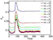
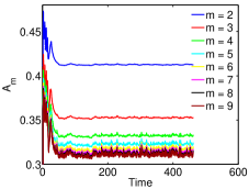
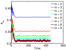
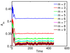
Figure 2: Plots of $A_{m}$ versus time for four forced simulations : in all of these $\max_{t}A_{m}<0.5$. Figs 2a-d are the result of pseudo-spectral $512^{3}$ simulations on a cubical $[0,\,2\pi]^{3}$-domain with random initial conditions. Fig 2a is the result of Kolmogorov forcing with $|\mathbi{f}_{0}|=0.005$ and $k_{1}=1$, while figs 2b-d are plots for three different values of $Re_{\lambda}$, namely $Re_{\lambda_{1,2,3}}=97,117$ and $192$ respectively, under the influence of white-noise forcing : see the text for a more detailed explanation.

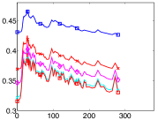
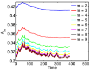
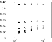
Figure 3: Plots 3a, b are of $A_{m}$ defined in (2.6) versus time for two decaying simulations for which $\max_{t}A_{m}<0.5$. Fig. 3a is a $1024\times 2048\times 512$ pseudo-spectral simulation on a long $4\pi\times 16\pi\times 2\pi$ domain with anti-parallel initial conditions [31, 1]. Fig. 3b is a decaying version of the $512^{3}$ simulation as in Figs. 2a-d. Fig. 3c is a plot of $\overline{A}_{m}$ defined by $\overline{A}_{m}=\ln\left<D_{m}\right>_{T}/\ln\left<D_{1}\right>_{T}$ arising from the TAMU database with the horizontal axis denoting values of $Re_{\lambda}$. Open and closed symbols denote results from two types of forcing (EP and FEK) for statistically steady flows : see [1].

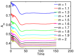
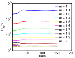
Figure 4: Example of a simulation with white-noise forcing, as in Fig. 2d ($Re_{\lambda}=192$) performed in the range $1\leq m\leq 2$. In the right-hand figure $D_{1}$ is included whereas it is not in Fig. 2d.

2.2 How to choose $\max_{t}A_{m}$

$\lambda$	1.1	1.15	1.2	1.25	1.3	1.35	1.4	1.45	1.5
$A_{2,\lambda}$	0.42	0.43	0.44	0.45	0.46	0.47	0.48	0.49	0.5
$A_{6,\lambda}$	0.31	0.32	0.33	0.35	0.36	0.36	0.38	0.39	0.40
$A_{9,\lambda}$	0.30	0.31	0.32	0.33	0.35	0.36	0.37	0.38	0.39

Table 1: Table of values of $\lambda$ and $A_{2,\lambda},~{}A_{6,\lambda}$ and $A_{9,\lambda}$ corresponding to Figs. 2 and 3.

The numerical experiments reported above show that $A_{m}$ has values lying in a wide range. Is there a way of choosing $\max_{t}A_{m}$ as a function of $m$ in a simple manner consistent with the results of these simulations? The following is a consistency argument based on the inequalities the $D_{m}$ must obey.

Firstly it is easy to prove that

$$\Omega_{m}^{m(p+q)}\leq\Omega_{m-p}^{q(m-p)}\Omega_{m+q}^{p(m+q)}\,.$$ (2.8)

Let $p=m-1$ and $q=1$ to give $\Omega_{m}^{m^{2}}\leq\Omega_{1}\Omega_{m+1}^{m^{2}-1}$. In terms of $D_{m}$, this translates to

$$D_{m}^{m^{2}}\leq D_{1}^{\alpha_{m}/2}D_{m+1}^{\alpha_{m}(m^{2}-1)/\alpha_{m+1}}\,.$$ (2.9)

Suppressing the $\lambda$-label on $A_{m+1}$ in the depletion $D_{m+1}\leq D_{1}^{A_{m+1}}$, we obtain

$$D_{m}\leq D_{1}^{\frac{1+A_{m+1}(m-1)(4m+1)}{m(4m-3)}}\,.$$ (2.10)

For the exponent on the right-hand side of (2.9) to be consistent with $D_{m}\leq D_{1}^{A_{m}}$, we require

$$\frac{1+A_{m+1}(m-1)(4m+1)}{m(4m-3)}=A_{m}\,.$$ (2.11)

By using the definition $\chi_{m}=A_{m}(4m-3)$, this reduces to

$$1+(m-1)\chi_{m+1}=m\chi_{m}\,,$$ (2.12)

which is solved to give :

Proposition 1

The solution of (2.12) is given by

$$\chi_{m,\lambda}=m\lambda+1-\lambda\,,\qquad\mbox{or}\qquad A_{m,\lambda}=\frac{m\lambda+1-\lambda}{4m-3}\,,$$ (2.13)

where the constant $\lambda$ lies in the range $1\leq\lambda\leq 4$.

The fit of (2.13) to the figures in §2.1 is not perfect in the sense that numerical trajectories do not follow exactly the concave curves of Fig. 1, so the appropriate value of $\lambda$ from an initial condition needs to be estimated. To achieve this, we label as $\lambda_{m}$ those values computed from $\max_{t}A_{m}$ in a given figure. These increase slightly with $m$ ; for example, in Fig 3a, $\lambda_{2}=1.4$ at $m=2$, whereas $\lambda_{9}=1.45$ at $m=9$ (see table 1). $\lambda_{\rm min}$, defined in (2.14), is taken as the minimum of a set of values of $\lambda$ computed over a range of $m$ from a given initial condition. This can then be used in the estimates for the attractor dimension or energy spectrum in the following sections.

$$\lambda_{\rm min}=\min\left\{\lambda_{m}\,:2\leq m\leq N\right\}\,.$$ (2.14)

$m$	1.1	1.5	1.9
$A_{m,\lambda}$	0.85	0.55	0.45
$\lambda$	1.5	1.3	1.19

Table 2: Table of values of $\lambda$ corresponding to $A_{1.1,\lambda},~{}A_{1.5,\lambda}$ and $A_{1.9,\lambda}$ corresponding to Fig. 4.

2.3 A division into three regimes

The scaling ansatz for $A_{m,\lambda}$ in (2.13) derived in Proposition 1 suggests that the $D_{1}-D_{m}$ plane can be divided into different regimes for the range $1\leq\lambda\leq 2$ :

Regime I : $D_{1}^{\frac{m}{4m-3}}\leq D_{m}\leq D_{1}^{A_{m,\lambda}}$ : the lower bound is $\Omega_{1}\leq\Omega_{m}$ expressed in the $D_{m}$-notation.

Regime II : $D_{1}^{A_{m,\lambda}}<D_{m}\leq C_{m}D_{1}$, where $C_{m}^{\eta_{m}}=\varpi_{2,m}/\varpi_{1,m}=c_{1,m}c_{2,m}$, and $\eta_{m}=\frac{2m}{3(m-1)}$.

Regime III : $C_{m}D_{1}<D_{m}$.

Regime III appears in the following way. Using the standard contradiction method, for $1<m<\infty$ ($\varpi_{i,m}$ are constants), the $D_{m}$ obey the differential inequality [35, 36]

$$\dot{D}_{m} \leq D_{m}^{3}\left\{-\varpi_{1,m}\left(\frac{D_{m+1}}{D_{m}}\right)^{\rho_{m}}+\varpi_{2,m}\right\}+\varpi_{3,m}GrD_{m}^{\frac{\alpha_{m}-1}{\alpha_{m}}}\,,$$ (2.15)

$$\rho_{m} = {\scriptstyle\frac{2}{3}}m(4m+1)\,.$$ (2.16)

Moreover, for $m>1$ it is easily proved that

$$\frac{D_{m}}{D_{1}}\leq\left(\frac{D_{m+1}}{D_{m}}\right)^{(m-1)(4m+1)}\,,$$ (2.17)

which changes (2.15) and (2.16) into

$$\dot{D}_{m} \leq D_{m}^{3}\left\{-\varpi_{1,m}\left(\frac{D_{m}}{D_{1}}\right)^{\eta_{m}}+\varpi_{2,m}\right\}+\varpi_{3,m}GrD_{m}^{\frac{\alpha_{m}-1}{\alpha_{m}}}\,,$$ (2.18)

$$\eta_{m} = \frac{2m}{3(m-1)}\,.$$ (2.19)

Clearly, in regime III the combination of terms within the braces is negative and can be neglected. In this regime the dissipation is sufficiently strong to control solutions rather than depletion reducing the nonlinearity. In the unforced case, the $D_{m}$ always decay ; at most, they grow only algebraically in time in the forced case (see §4). Moreover, $\Omega_{1}\leq\Omega_{m}$ universally implies that

$$\left(\frac{D_{m}}{D_{1}}\right)^{\eta_{m}}D_{m}^{2}\geq 1\,,$$ (2.20)

which means that $D_{m}\geq 1$ in regime I, while in regime II there is a lower bound $D_{m}^{2}\geq C_{m}^{-\eta_{m}}$.

3 Regime I

3.1 Depletion resulting in an absorbing ball for $D_{1}$

It has long been understood that the $H_{1}$-norm of the velocity field ($D_{1}$ in the notation of this paper) controls all the regularity properties of $3D$ Navier-Stokes equations [10, 11, 12, 13]. It is also the essential missing ingredient in the search for the proof of the existence of a $3D$ Navier-Stokes global attractor. What is required is an “absorbing ball” for this norm, which consists of a ball of finite radius into which all solutions are drawn for large times. In what follows, estimates are made for the forced case in terms of the Grashof number $Gr$ or Reynolds number $Re$. In the unforced case the conclusions regarding the finiteness of $D_{1}$ still stand except that the radius of the ball decays and the attractor is just the origin.

In this context it is difficult to handle a wide variety of forcing functions analytically. For simplicity we shall remain with the properties of the forcing as in Doering and Foias [46] who took forcing at a single scale $\ell$, taken here to be the box-scale $L$, to make estimates in terms of the Grashof number $Gr$ or Reynolds number $Re$ defined in (2.2).

The first task is to illustrate why the standard estimate for $D_{1}$ produces an apparently unsurmountable problem. Note that from the definition of the $D_{m}$ in (1.1) $D_{1}=L\nu^{-2}\|\mbox{\boldmath$\omega$}\|_{2}^{2}$ so, using the standard contradiction method (see footnote 10), a formal differential inequality for $D_{1}$ is

$${\scriptstyle\frac{1}{2}}\dot{D}_{1}\leq L\nu^{-2}\left\{-\nu\int_{\mathcal{V}}|\nabla\mbox{\boldmath$\omega$}|^{2}\,dV+\int_{\mathcal{V}}|\nabla\mbox{\boldmath$u$}||\mbox{\boldmath$\omega$}|^{2}\,dV+L^{-1}\left(\int_{\mathcal{V}}|\mbox{\boldmath$\omega$}|^{2}\,dV\right)^{1/2}\|\mathbi{f}\|_{2}\right\}\,.$$ (3.1)

Dealing with the negative term first, an integration by parts gives

$$\int_{\mathcal{V}}|\mbox{\boldmath$\omega$}|^{2}\,dV\leq\left(\int_{\mathcal{V}}|\nabla\mbox{\boldmath$\omega$}|^{2}dV\right)^{1/2}\left(\int_{\mathcal{V}}|\mbox{\boldmath$u$}|^{2}dV\right)^{1/2}\,,$$ (3.2)

where the dimensionless energy $E$ is defined as

$$E=\nu^{-2}L^{-1}\int_{\mathcal{V}}|\mbox{\boldmath$u$}|^{2}\,dV\,.$$ (3.3)

which is always bounded such that [10-13]

$$\overline{\lim}_{t\to\infty}E\leq c\,Gr^{2}\,.$$ (3.4)

Then the nonlinear term in (3.1) can be estimated in two ways :

1. By using a Sobolev inequality in the standard way [10-13] ;

2. By invoking the nonlinear depletion of regime I.

(1) The standard method simply involves a Schwarz inequality to estimate the nonlinear term as

$$\int_{\mathcal{V}}|\nabla\mbox{\boldmath$u$}||\mbox{\boldmath$\omega$}|^{2}\,dV\leq\|\mbox{\boldmath$\omega$}\|_{2}\|\mbox{\boldmath$\omega$}\|_{4}^{2}\,.$$ (3.5)

After the application of the Sobolev inequality $\|\mbox{\boldmath$\omega$}\|_{4}\leq c\,\|\nabla\mbox{\boldmath$\omega$}\|_{2}^{3/4}\|\mbox{\boldmath$\omega$}\|_{2}^{1/4}$, this becomes

$$\int_{\mathcal{V}}|\nabla\mbox{\boldmath$u$}||\mbox{\boldmath$\omega$}|^{2}\,dV \leq c\,\|\nabla\mbox{\boldmath$\omega$}\|_{2}^{3/2}\|\mbox{\boldmath$\omega$}\|_{2}^{3/2}$$ (3.6)

$$\leq \frac{3\nu}{4}\|\nabla\mbox{\boldmath$\omega$}\|_{2}^{2}+\frac{c}{4\nu^{3}}\|\mbox{\boldmath$\omega$}\|_{2}^{6}\,.$$

(3.1) then becomes

$${\scriptstyle\frac{1}{2}}\dot{D}_{1}\leq\varpi_{0}\left(-\frac{1}{4}\frac{D_{1}^{2}}{E}+c\,D_{1}^{3}+GrD_{1}^{1/2}\right)\,.$$ (3.7)

Clearly the cubic nonlinearity is too strong for the quadratic negative term : all we can deduce is that $D_{1}$ is bounded from above only for short times or for small initial data. The difficulty caused by this term has been known for many decades : see [10, 11, 12, 13] and also Lu and Doering [37].

(2) Now we turn to using the nonlinear depletion of regime I. How might the insertion of $D_{m}\leq D_{1}^{A_{m,\lambda}}$ mollify the cubic exponent in (3.7)? We return to (3.1) and estimate the nonlinear term as

$$\int_{\mathcal{V}}|\nabla\mbox{\boldmath$u$}||\mbox{\boldmath$\omega$}|^{2}dV = \int_{\mathcal{V}}|\mbox{\boldmath$\omega$}|^{\frac{2m-3}{m-1}}|\mbox{\boldmath$\omega$}|^{\frac{1}{m-1}}|\nabla\mbox{\boldmath$u$}|dV$$ (3.8)

$$\leq \left(\int_{\mathcal{V}}|\mbox{\boldmath$\omega$}|^{2}dV\right)^{\frac{2m-3}{2(m-1)}}\left(\int_{\mathcal{V}}|\mbox{\boldmath$\omega$}|^{2m}dV\right)^{\frac{1}{2m(m-1)}}\left(\int_{\mathcal{V}}|\nabla\mbox{\boldmath$u$}|^{2m}dV\right)^{\frac{1}{2m}}$$

$$\leq c_{m}\left(\int_{\mathcal{V}}|\mbox{\boldmath$\omega$}|^{2}dV\right)^{\frac{2m-3}{2(m-1)}}\left(\int_{\mathcal{V}}|\mbox{\boldmath$\omega$}|^{2m}dV\right)^{\frac{1}{2(m-1)}}$$

$$= c_{m}L^{3}\varpi_{0}^{3}D_{1}^{\frac{2m-3}{2m-2}}D_{m}^{\frac{4m-3}{2m-2}}\,,\qquad\qquad 1<m<\infty\,.$$

based on $\|\nabla\mbox{\boldmath$u$}\|_{p}\leq c_{p}\|\mbox{\boldmath$\omega$}\|_{p}$, for $1<p<\infty$. Inserting the depletion $D_{m}\leq D_{1}^{A_{m,\lambda}}$,

$$L\nu^{-2}\int_{\mathcal{V}}|\nabla\mbox{\boldmath$u$}||\mbox{\boldmath$\omega$}|^{2}\,dV\leq c_{m}\varpi_{0}D_{1}^{\xi_{m,\lambda}}\,,$$ (3.9)

where $\xi_{m,\lambda}$ is defined as in (1.5) but repeated here

$$\xi_{m,\lambda}=\frac{\chi_{m,\lambda}+2m-3}{2(m-1)}\,,\qquad\qquad\chi_{m,\lambda}=A_{m,\lambda}(4m-3)=m\lambda+1-\lambda\,.$$ (3.10)

Thus we have

$$\xi_{m,\lambda}=1+{\scriptstyle\frac{1}{2}}\lambda\,,$$ (3.11)

which is explicitly $m$-independent. Thus the equivalent of (3.7) is

$$\boxed{{\scriptstyle\frac{1}{2}}\dot{D}_{1}\leq\varpi_{0}\left(-\frac{D_{1}^{2}}{E}+c_{m}D_{1}^{1+{\scriptstyle\frac{1}{2}}\lambda}+GrD_{1}^{1/2}\right)\,.}$$ (3.12)

Given that $E$ is bounded above, $D_{1}$ is always under control provided $\lambda$ is restricted to the range $1\leq\lambda<2$. This is expressed in the following :

Proposition 2

If the solution always remains in regime I ($1\leq\lambda<2$), there exists an absorbing ball for $D_{1}$ of radius

$$\overline{\lim}_{t\to\infty}D_{1}\leq c_{m}Gr^{\frac{4}{2-\lambda}}+O\left(Gr^{4/3}\right)\,.$$ (3.13)

Remark 1 : The range of control over $D_{1}$ in $1\leq\lambda<2$ can be extended to $\lambda=2$ as (3.12) shows that there is an exponentially growing bound on $D_{1}$ at this value.

Remark 2 : Note that the values of $\lambda=\lambda_{\rm min}$ corresponding to the numerical experiments in §2 lie well within the range ($1\leq\lambda<2$) of validity, as illustrated by Fig. 1.

Remark 3 : From (3.13) and the standard properties of the Navier-Stokes equations [10, 11, 12, 13], we conclude that a global attractor $\mathcal{A}$ exists in this regime, which is a compact $L^{2}$-bounded ball for the velocity field $u$. $c_{m}$ is a generic constant dependent only on $m$.

3.2 An estimate for the attractor dimension

It is now possible to estimate the Lyapunov dimension of the global attractor $\mathcal{A}$, which has been shown to exist as a result of Proposition 2, subject to the depletion in regime I. A connection between the system dynamics and the attractor dimension is provided by the notion of the Lyapunov exponents through the Kaplan-Yorke formula. For ODEs the Lyapunov exponents control the exponential growth or contraction of volume elements in phase space : the Kaplan-Yorke formula expresses the balance between volume growth and contraction realized on the attractor. It has been rigorously applied to global attractors in PDEs by Constantin and Foias [47, 10] : see also [11, 12, 48]. The formula is the following : for Lyapunov exponents labelled in descending order and designated by $\mu_{n}$, the Lyapunov dimension $d_{L}$ is defined in terms of these by

$$d_{L}=N-1+\frac{\mu_{1}+\ldots+\mu_{N-1}}{-\mu_{N}},$$ (3.14)

where the number $N$ of $\mu_{n}$ is chosen to satisfy

$$\sum_{n=1}^{N-1}\mu_{n}\geq 0\hskip 28.45274pt\mbox{but}\hskip 28.45274pt\sum_{n=1}^{N}\mu_{n}<0\,.$$ (3.15)

Note that according to the definition of $N$, the ratio of exponents in (3.14) satisfies

$$0\leq\frac{\mu_{1}+\ldots+\mu_{N-1}}{-\mu_{N}}<1\,,$$ (3.16)

so the formula generally yields a non-integer dimension such that

$$N-1\leq d_{L}<N\,.$$ (3.17)

The value of $N$ that turns the sign of the sum of the Lyapunov exponents, as in (3.15), is that value of $N$ that bounds above $d_{L}$ and hence the Hausdorff and fractal dimensions $d_{H}$ and $d_{F}$. For a discussion of generalized dimensions see the paper by Hentschel and Procaccia [49]. To use the method for PDEs as developed in [47, 10] the phase space is replaced by $\mbox{\boldmath$u$}\in L^{2}\cap\mbox{div}\,\mbox{\boldmath$u$}=0$, which is infinite dimensional. The solution $\mbox{\boldmath$u$}(t)$ forms an orbit in this space, with different sets of initial conditions $\mbox{\boldmath$u$}(0)+\delta\mbox{\boldmath$u$}_{i}(0)$, which evolve into $\mbox{\boldmath$u$}(t)+\delta\mbox{\boldmath$u$}_{i}(t)$ for $i=1,\ldots,N$. The linearized form of the Navier-Stokes equations in terms of $\delta\mbox{\boldmath$u$}$ of $u$ is

$$\partial_{t}(\delta\mbox{\boldmath$u$})+\mbox{\boldmath$u$}\cdot\nabla\delta\mbox{\boldmath$u$}+\delta\mbox{\boldmath$u$}\cdot\nabla\mbox{\boldmath$u$}=\nu\Delta\delta\mbox{\boldmath$u$}-\nabla\delta p\,,$$ (3.18)

which can also be written in the form

$$\partial_{t}(\delta\mbox{\boldmath$u$})=\mathcal{M}\delta\mbox{\boldmath$u$}\,.$$ (3.19)

If they are chosen to be linearly independent, initially these $\delta\mbox{\boldmath$u$}_{i}$ form an $N$-volume or parallelpiped of volume

$$V_{N}(t)=\left|\delta\mbox{\boldmath$u$}_{1}\wedge\delta\mbox{\boldmath$u$}_{2}\ldots\wedge\delta\mbox{\boldmath$u$}_{N}\right|\,.$$ (3.20)

It is now necessary to find the time evolution of $V_{N}$. This is given by

$$\dot{V}_{N}=V_{N}Tr\left[\mathbf{P}_{N}\mathcal{M}\mathbf{P}_{N}\right]\,,$$ (3.21)

which is easily solved to give

$$V_{N}(t)=V_{N}(0)\exp\int_{0}^{t}Tr\left[\mathbf{P}_{N}\mathcal{M}\mathbf{P}_{N}\right](\tau)\,d\tau\,.$$ (3.22)

$\mathbf{P}_{N}(t)$ is an $L^{2}$-orthogonal projection, using the orthonormal set of functions $\{\mbox{\boldmath$\phi$}_{i}\}$, onto the finite dimensional subspace $\mathbf{P}_{N}L^{2}$, which spans the set of vectors $\delta\mbox{\boldmath$u$}_{i}$ for $i=1,\,...,\,N$. In terms of the time average $\left<\cdot\right>_{t}$ up to time $t$, the sum of the first $N$ global Lyapunov exponents is taken to be [47, 10]

$$\sum_{n=1}^{N}\mu_{n}=\left<Tr\left[\mathbf{P}_{N}\mathcal{M}\mathbf{P}_{N}\right]\right>_{t}\,.$$ (3.23)

As in (3.15), we want to find the value of $N$ that turns the sign of $\left<Tr\left[\mathbf{P}_{N}\mathcal{M}\mathbf{P}_{N}\right]\right>_{t}$ and for which volume elements contract to zero. This value of $N$ bounds above $d_{L}$ as in (3.14). To estimate this we write

$$Tr\left[\mathbf{P}_{N}{\cal M}\mathbf{P}_{N}\right]=\sum_{n=1}^{N}\int_{\mathcal{V}}\mbox{\boldmath$\phi$}_{n}\cdot\left\{\nu\Delta\mbox{\boldmath$\phi$}_{n}-\mbox{\boldmath$u$}\cdot\nabla\mbox{\boldmath$\phi$}_{n}-\mbox{\boldmath$\phi$}_{n}\cdot\nabla\mbox{\boldmath$u$}-\nabla\tilde{p}\left(\mbox{\boldmath$\phi$}_{n}\right)\right\}\,dV.$$ (3.24)

Since $\mbox{div}\,\delta_{m}\mbox{\boldmath$u$}_{n}=0$ for all $n$, then $\mbox{div}\,\mbox{\boldmath$\phi$}_{n}=0$ also and so the pressure term integrates away, as does the second term

$$Tr\left[\mathbf{P}_{N}{\cal M}\mathbf{P}_{N}\right]\leq-\nu\sum_{n=1}^{N}\int_{\mathcal{V}}|\nabla\mbox{\boldmath$\phi$}_{n}|^{2}\,dV+\sum_{n=1}^{N}\int_{\mathcal{V}}|\nabla\mbox{\boldmath$u$}|\,|\mbox{\boldmath$\phi$}_{n}|^{2}\,dV.$$ (3.25)

Because the $\mbox{\boldmath$\phi$}_{n}$ are orthonormal they obey the relations

$$\sum_{n=1}^{N}\int_{\mathcal{V}}|\mbox{\boldmath$\phi$}_{n}|^{2}\,dV=N,\hskip 28.45274pt\mbox{and}\hskip 28.45274ptTr\left[\mathbf{P}_{N}(-\Delta)\mathbf{P}_{N}\right]=\sum_{n=1}^{N}\int_{\mathcal{V}}|\nabla\mbox{\boldmath$\phi$}_{n}|^{2}\,dV.$$ (3.26)

In $3D$ the $\mbox{\boldmath$\phi$}_{n}$ satisfy the Lieb-Thirring inequalities [47, 10, 13, 11] for orthonormal functions

$$\int_{\mathcal{V}}\left(\sum_{n=1}^{N}|\mbox{\boldmath$\phi$}_{n}|^{2}\right)^{5/3}\!\!dV\leq c\,\sum_{n=1}^{N}\int_{\mathcal{V}}|\nabla\mbox{\boldmath$\phi$}_{n}|^{2}\,dV,$$ (3.27)

where $c$ is independent of $N$. Moreover, it is known that the first $N$ eigenvalues of the Stokes operator in three-dimensions satisfy

$$Tr\left[\mathbf{P}_{N}(-\Delta)\mathbf{P}_{N}\right]\geq c\,N^{5/3}L^{-2}\,.$$ (3.28)

To exploit the Lieb-Thirring inequality (3.27) to estimate the last term in (3.25) we write it as

$$\sum_{n=1}^{N}\int_{\mathcal{V}}|\nabla\mbox{\boldmath$u$}|\,|\mbox{\boldmath$\phi$}_{n}|^{2}\,dV\leq\left[\int_{\mathcal{V}}|\nabla\mbox{\boldmath$u$}|^{5/2}\,dV\right]^{2/5}\,\left[\int_{\mathcal{V}}\left(\sum_{n=1}^{N}|\mbox{\boldmath$\phi$}_{n}|^{2}\right)^{5/3}\!dV\right]^{3/5}.$$ (3.29)

Hence, using (3.27) and time averaging $\left<\cdot\right>_{t}$, we find

$$\left<\sum_{n=1}^{N}\int_{\mathcal{V}}|\nabla\mbox{\boldmath$u$}|\,|\mbox{\boldmath$\phi$}_{n}|^{2}\,dV\right>_{t} \leq c\,\left<\left(Tr\left[\mathbf{P}_{N}(-\Delta)\mathbf{P}_{N}\right]\right)^{3/5}\left(\int_{\mathcal{V}}|\nabla\mbox{\boldmath$u$}|^{5/2}\,dV\right)^{2/5}\right>_{t}$$ (3.30)

$$\leq \frac{3\nu}{5}\left<Tr\left[\mathbf{P}_{N}(-\Delta)\mathbf{P}_{N}\right]\right>_{t}+\frac{2c}{5\nu^{3/2}}\left<\int_{\Omega}|\nabla\mbox{\boldmath$u$}|^{5/2}\,dV\right>_{t}$$

and so (3.25) can be written as

$$\left<Tr\left[\mathbf{P}_{N}{\cal M}\mathbf{P}_{N}\right]\right>_{t}\leq-\frac{2}{5}\nu\left<Tr\left[\mathbf{P}_{N}(-\Delta)\mathbf{P}_{N}\right]\right>_{t}+\frac{2}{5}c\,\nu^{-3/2}\left<\int_{\mathcal{V}}|\nabla\mbox{\boldmath$u$}|^{5/2}\,dV\right>_{t}\,.$$ (3.31)

To estimate the nonlinear term we use Hölder’s inequality to obtain ($m>1$)

$$\int_{\mathcal{V}}\left|\nabla\mbox{\boldmath$u$}\right|^{5/2}\,dV \leq c\,\int_{\mathcal{V}}|\mbox{\boldmath$\omega$}|^{5/2}\,dV$$ (3.32)

$$\leq c\,\left(\int_{\mathcal{V}}|\mbox{\boldmath$\omega$}|^{2}\,dV\right)^{\frac{4m-5}{4(m-1)}}\left(\int_{\mathcal{V}}|\mbox{\boldmath$\omega$}|^{2m}\,dV\right)^{\frac{1}{4(m-1)}}$$

$$\leq c\,\varpi_{0}^{5/2}L^{3}D_{1}^{\frac{4m-5}{4(m-1)}}D_{m}^{\frac{4m-3}{4(m-1)}}\,.$$

Therefore, using this and (3.28), we find

$$\varpi_{0}^{-1}\left<Tr\left[\mathbf{P}_{N}{\cal M}\mathbf{P}_{N}\right]\right>_{t}\leq-c_{1}N^{5/3}+c_{2}\left<D_{1}^{\frac{4m-5}{4(m-1)}}D_{m}^{\frac{4m-3}{4(m-1)}}\right>_{t}\,.$$ (3.33)

It is at this point where the depletion of nonlinearity $D_{m}\leq D_{1}^{A_{m,\lambda}}$ is used, thereby giving

$$\left<D_{1}^{\frac{4m-5}{4(m-1)}}D_{m}^{\frac{4m-3}{4(m-1)}}\right>_{t}\leq\left<D_{1}\right>_{t}\left(\overline{\lim}_{t\to\infty}D_{1}\right)^{\frac{\chi_{m,\lambda}-1}{4(m-1)}}\,,$$ (3.34)

where $\chi_{m,\lambda}=A_{m,\lambda}(4m-3)$ as defined in (1.5). Proposition 2 and the estimate $\left<D_{1}\right>_{t}\leq c\,GrRe$ from [46] then allow us to write

$$\left<D_{1}\right>_{t}\left(\overline{\lim}_{t\to\infty}D_{1}\right)^{\frac{\chi_{m,\lambda}-1}{4(m-1)}}\leq c\,(GrRe)Gr^{\frac{\chi_{m,\lambda}-1}{2m-1-\chi_{m,\lambda}}}\leq c\,Re^{\frac{6m-5-\chi_{m,\lambda}}{2m-1-\chi_{m,\lambda}}}\,,$$ (3.35)

and so (3.33) can be written as

$$\left<Tr\left[\mathbf{P}_{N}{\cal M}\mathbf{P}_{N}\right]\right>_{t}\leq\varpi_{0}\left(-c_{1}N^{5/3}+c_{2}Re^{\frac{6m-5-\chi_{m,\lambda}}{2m-1-\chi_{m,\lambda}}}\right)\,.$$ (3.36)

To find an estimate solely in terms of $Gr$ the $(GrRe)$-term of (3.35) is replaced by $Gr^{2}$. Choosing $\chi_{m,\lambda}$ as in (2.13), we have proved :

Proposition 3

If the solution always remains in regime I the Lyapunov dimension of the global attractor $\mathcal{A}$ is estimated as

$$d_{L}(\mathcal{A})\leq c_{1,m}Re^{\frac{3}{5}\left(\frac{6-\lambda}{2-\lambda}\right)}\,,$$ (3.37)

or, alternatively, as

$$d_{L}(\mathcal{A})\leq c_{2,m}Gr^{\frac{3}{5}\left(\frac{4-\lambda}{2-\lambda}\right)}\,.$$ (3.38)

4 Regimes II and III

In §3, regime I has been defined to lie in the region $D_{m}\leq D_{1}^{A_{m,\lambda}}$ for $1\leq\lambda<2$, with regime II defined as the region where this inequality has been reversed up to $C_{m}D_{1}$. One could fuse regimes I and II together by taking $\lambda$ in the wider range $1\leq\lambda\leq 4$ but we have no control over $D_{1}$ for $2<\lambda\leq 4$. In this section we choose to remain with the definition of regime II as in (1).

To test whether there is any depletion in regime II let us repeat inequality (3.8) for the nonlinear term and use $D_{m}\leq C_{m}D_{1}$

$$\int_{\mathcal{V}}|\nabla\mbox{\boldmath$u$}||\mbox{\boldmath$\omega$}|^{2}\,dV \leq c\,L^{3}\varpi_{0}^{3}D_{1}^{\frac{2m-3}{2m-2}}D_{m}^{\frac{4m-3}{2m-2}}$$ (4.1)

$$\leq c\,L^{3}\varpi_{0}^{3}C_{m}^{\frac{4m-3}{2m-2}}D_{1}^{3}\,.$$

Thus $\xi_{m,4}=3$ and there is no depletion of nonlinearity in the upper bound $D_{m}\leq C_{m}D_{1}$. Moreover, when the scaling argument in §2.2 is repeated, this too shows no depletion. To test whether the dissipation term in (2.18) is changed by the use of the lower bound $D_{1}^{A_{m,\lambda}}<D_{m}$ we consider first (2.20)

$$D_{m}^{2}\left(\frac{D_{m}}{D_{1}}\right)^{\eta_{m}}>D_{1}^{A_{m,\lambda}(2+\eta_{m})-\eta_{m}}\equiv D_{1}^{\Delta_{m,\lambda}}\,,$$ (4.2)

which improves the lower bound of unity in (2.20) and thereby increases the dissipation. In fact

$$\Delta_{m,\lambda}=\frac{2}{3}(\lambda-1)\,.$$ (4.3)

Let us assume that initial data is placed in regime II at a time $t_{0}$ : then dividing (2.18) by $D_{m}^{3}$ we find

$${\scriptstyle\frac{1}{2}}\frac{d~{}}{dt}D_{m}^{-2}\geq D_{m}^{-2}\left\{\varpi_{1,m}D_{1}^{\Delta_{m,\lambda}}\right\}-\varpi_{2,m}\,,$$ (4.4)

where, for convenience, we have taken the unforced case [35]. An integration over $[t_{0},\,t]$ gives

$$e^{-(t-t_{0})g(t)}D_{m}^{-2}(t)\geq D_{m}^{-2}(t_{0})-2\varpi_{2,m}\int_{t_{0}}^{t}e^{-(\tau-t_{0})g(\tau)}\,d\tau$$ (4.5)

where

$$g(t)=\frac{2\varpi_{1,m}}{t-t_{0}}\int_{t_{0}}^{t}D_{1}^{\Delta_{m,\lambda}}\,d\tau\,.$$ (4.6)

The main question here is whether there exists a sufficiently large lower bound on the time average $g(t)$ to prove that the right hand side of (4.5) never develops a zero for some wide range of initial data? The problem is that the size of $\int_{t_{0}}^{t}D_{1}^{\Delta_{m,\lambda}}d\tau$ over very short intervals $[t_{0},\,t]$ is indeterminate. This lower bound would have to be large enough on arbitrarily small intervals for the negative integral of the exponential in (4.5) to be always smaller than $D_{m}^{-2}(t_{0})$ to prevent a zero forming on the right-hand side.

Finally, regime III is easily dealt with because the condition $C_{m}D_{1}<D_{m}$ allows us to drop two of the three terms in the (2.18) leaving us with $\dot{D}_{m}\leq 0$ in the unforced case, thus implying decay from initial data. In the forced case $\dot{D}_{m}\leq\varpi_{3,m}GrD_{m}^{1-1/\alpha_{m}}$ and so it follows that any $D_{m}$ that satisfies this is bounded for all time as in

$$D_{m}\leq\left[D_{m}^{\alpha_{m}^{-1}}(t_{0})+\alpha_{m}^{-1}\varpi_{3,m}Gr\left(t-t_{0}\right)\right]^{\alpha_{m}}$$ (4.7)

5 Energy spectra and typical length scales in regimes I & II

Some ideas are explained in this section on how information might be extracted from the analysis on the properties of an energy spectrum $\mathcal{E}(k)$ corresponding to regimes I and II. Doering and Gibbon [44] have shown how to associate bounds of time averages with the moments of this spectrum by following some ideas in [2, 45]. It is these arguments we shall summarize first.

In the standard manner, we define

$$H_{n}(t)=\int_{\mathcal{V}}|\nabla^{n}\mbox{\boldmath$u$}|^{2}\,dV\qquad\mbox{with}\qquad H_{0}=\int_{\mathcal{V}}|\mbox{\boldmath$u$}|^{2}\,dV\,,$$ (5.1)

where the label $n$ refers to derivatives. Then it was shown in [44] that to take proper account of the forcing these require an additive adjustment such that

$$F_{n}=H_{n}+\tau^{2}\|\nabla^{n}\mathbi{f}\|_{2}^{2}\,,$$ (5.2)

where $\tau^{-1}\sim\varpi_{0}Gr^{{\scriptstyle\frac{1}{2}}+\varepsilon}$ for any $\varepsilon>0$. This formalism now allows us to define the set of ‘wave-numbers’ $\kappa_{n,0}$ and $\kappa_{n,1}$ such that

$$\kappa_{n,0}^{2n}=F_{n}/F_{0}\,,\qquad\qquad\kappa_{n,1}^{2(n-1)}=F_{n}/F_{1}\,.$$ (5.3)

Using the fact that

$${\scriptstyle\frac{1}{2}}\dot{H}_{1}\leq-\nu H_{2}+\int_{\mathcal{V}}|\nabla\mbox{\boldmath$u$}||\mbox{\boldmath$\omega$}|^{2}dV+\mbox{forcing}\,,$$ (5.4)

which is just another way of expressing (3.1), we can re-visit the inequality in (3.8) to estimate the integral in (5.4) with the application of the depletion of regime I

$$\int_{\mathcal{V}}|\nabla\mbox{\boldmath$u$}||\mbox{\boldmath$\omega$}|^{2}dV\leq\varpi_{0}\left(L^{3}\varpi_{0}^{2}\right)^{1-\xi_{m,\lambda}}H_{1}^{\xi_{m,\lambda}}=\varpi_{0}H_{1}D_{1}^{\xi_{m,\lambda}-1}\,,$$ (5.5)

which, again, is just another expression of (3.9). The bounds $1\leq\lambda<2$ mean that

$$3/2\leq\xi_{m,\lambda}<2\,,$$ (5.6)

and so

$${\scriptstyle\frac{1}{2}}\dot{H}_{1}\leq\varpi_{0}\left\{-L^{2}H_{2}+H_{1}D_{1}^{\xi_{m,\lambda}-1}\right\}+\mbox{forcing}\,,$$ (5.7)

which, when the $H_{n}$ are adjusted to the $F_{n}$ defined in (5.2) as in [44], becomes

$${\scriptstyle\frac{1}{2}}\dot{F}_{1}\leq\varpi_{0}\left\{-L^{2}F_{2}+F_{1}D_{1}^{\xi_{m,\lambda}-1}\right\}+c_{n}\varpi_{0}Gr\,F_{1}\,.$$ (5.8)

Dividing (5.8) by $F_{1}$ and time averaging, we get [44]

$$L^{2}\left<\kappa_{2,1}^{2}\right>_{T}\leq\left<D_{1}\right>_{T}^{\xi_{m,\lambda}-1}\leq c\,Re^{3\left(\xi_{m,\lambda}-1\right)}\,.$$ (5.9)

Moreover, we can also write

$$\left<\kappa_{2,0}\right>_{T}\leq\left<\kappa_{2,1}\kappa_{1,0}\right>_{T}^{1/2}\leq\left<\kappa_{2,1}^{2}\right>_{T}^{1/4}\left<\kappa_{1,0}^{2}\right>_{T}^{1/4}\,.$$ (5.10)

In [44] it was shown that Leray’s energy inequality leads to an estimate for $L^{2}\left<\kappa_{1,0}^{2}\right>_{T}\leq Re^{1+\varepsilon}$, although from now on we ignore the infinitesimal $\varepsilon>0$. We combine this with (5.10) to show that

$$\left<\kappa_{2,0}\right>_{T}\leq c\,Re^{\sigma_{m,\lambda}}+O\left(Gr^{1/4}\right)\,,$$ (5.11)

where

$$\sigma_{m,\lambda}=\frac{3(\chi_{m,\lambda}-1)+2(m-1)}{8(m-1)}=(3\lambda+2)/8\,.$$ (5.12)

To interpret this estimate physically in terms of statistical turbulence theory (restricting attention to forcing at the longest wavelength $\ell=L$), suppose that $Gr$ is high enough and the resulting flow is turbulent, ergodic and isotropic enough in the limit $T\to\infty$ that the wave-numbers $\left<\kappa_{n,0}\right>_{T}$ may be identified with the moments of the energy spectrum $\mathcal{E}(k)$ according to

$$\left<\kappa_{n,0}\right>_{T}:=\left(\frac{\int_{L^{-1}}^{\infty}k^{2n}\mathcal{E}(k)\,dk}{\int_{L^{-1}}^{\infty}\mathcal{E}(k)\,dk}\right)^{1/2n}\,.$$ (5.13)

The a priori constraints on $\mathcal{E}(k)$ are that the velocity $U$ and energy dissipation rate $\epsilon$ obey

$$U^{2}=\int_{L^{-1}}^{\infty}\mathcal{E}(k)\,dk\hskip 56.9055pt\epsilon=\int_{L^{-1}}^{\infty}\nu k^{2}\mathcal{E}(k)\,dk\,.$$ (5.14)

Suppose also that $\mathcal{E}(k)$ displays an “inertial range” in the sense that it scales with a power of $k$ up to an effective cut-off wavenumber $k_{c}$. For simplicity, let us write

$$\mathcal{E}(k)=\left\{\begin{array}[]{cr}A\,k^{-q},&\ \ \ L^{-1}\leq k\leq k_{c}\,,\\ 0,&k>k_{c}\,,\end{array}\right.$$ (5.15)

We also assume that $k_{c}$ diverges as $\nu\to 0$, while $U^{2}$ and $\epsilon$ remain finite, and that $A$ depends only upon the energy flux $\epsilon$ and the outer length scale $\ell=L$. Then we have the asymptotic relations

$$\epsilon\sim\frac{U^{3}}{L}\hskip 28.45274pt\mbox{and}\hskip 28.45274ptLk_{c}\sim\left(\frac{\epsilon}{\nu^{3}}\right)^{\frac{1}{9-3q}}L^{\frac{4}{9-3q}}\sim Re^{\frac{1}{3-q}}\,.$$ (5.16)

Then the moments of the spectrum $\left<\kappa_{n,0}\right>_{T}$ satisfy

$$L\left<\kappa_{n,0}\right>_{T}\sim(L\,k_{c})^{1-\frac{q-1}{2n}}\sim Re^{\frac{1}{3-q}-\frac{1}{2n}\left(\frac{q-1}{3-q}\right)}\,.$$ (5.17)

Now let us compare this scaling result with the estimate in (5.11) for $n=2$ with $q=q_{m,\lambda}$ : this correspondence tells us that

$$q_{m,\lambda}=\frac{12\sigma_{m,\lambda}-5}{4\sigma_{m,\lambda}-1}\,,\qquad\mbox{with}\qquad q_{m,\lambda}=3-\frac{4}{3\lambda}\,.$$ (5.18)

In fact, for regime I, $q_{m,\lambda}$ lies between

$$5/3\leq q_{m,\lambda}<7/3\,.$$ (5.19)

The 5/3 at the lower end is the conventional Kolmogorov result which rises to just under 7/3. The cut-off of the inertial range as (5.15) is given by

$$Lk_{c}\sim Re^{1/(3-q)}\qquad\mbox{so}\qquad Lk_{c,\lambda}\sim Re^{3\lambda/4}\,.$$ (5.20)

A resolution length is inbuilt into this formalism : the estimate for $L\left<\kappa_{2,0}\right>_{T}$, with an exponent of $\sigma_{m}$, can be interpreted as an average length scale. Thus, the first $L\left<\kappa_{1,0}\right>_{T}$ is followed by an estimate for $L\left<\kappa_{2,0}\right>_{T}$ at $\chi_{m,\lambda}=m\lambda+1-\lambda$ :

$$L\left<\kappa_{1,0}\right>_{T}\leq Re^{1/2}\,,\qquad\qquad L\left<\kappa_{2,0,\lambda}\right>_{T}\leq Re^{\sigma_{m,\lambda}}\,,$$ (5.21)

where $\sigma_{m,\lambda}$ is defined as in (5.12). This is roughly consistent with scaling arguments found in other parts of the literature [50, 28].

In regime II we are forced to revert to the weak solution results in [44] where it was shown that for $n\geq 2$,

$$\left<\kappa_{n,0}\right>_{T}\leq c\,Re^{3-\frac{5}{2n}}\,.$$ (5.22)

For $n=2$ this means $\sigma_{m,\lambda}=7/4$ and thus $q_{m,\lambda}=8/3$. Table 3 summarizes the results for both regimes I and II.

$\lambda$	$1$	$2$	$4$
$\sigma_{m,\lambda}=(3\lambda+2)/8$	$5/8$	$1$	7/4
$q_{m,\lambda}=3-4/3\lambda$	$5/3$	7/3	8/3
$Lk_{c}\leq Re^{3\lambda/4}$	$Re^{3/4}$	$Re^{3/2}$	$Re^{3}$

Table 3: The entries in the second and third columns are the lower and upper bounds of $\sigma_{m,\lambda},~{}q_{m,\lambda}$ and $Lk_{c}$ corresponding to the two concave curves in Fig. 1. The fourth column lists values of these at $\lambda=4$, which is near the extreme end of regime II.

Interestingly, Sulem and Frisch [45] showed that a $k^{-8/3}$ energy spectrum is the borderline steepness capable of sustaining an energy cascade. This spectrum corresponds to the extreme limit, where the energy dissipation is concentrated on sets of dimension zero (points) in space [51, 52]. It provides some physical setting in which to interpret the result of Caffarelli, Kohn & Nirenberg that the space-time dimension of the Navier-Stokes singular set is unity [53].

6 Conclusion

Three regimes have been identified based on the size of the $D_{m}$ for $m\geq 2$ relative to that of $D_{1}$. Regime I has been shown to have a sufficiently depleted nonlinearity that an absorbing ball exists for $D_{1}$. The consequence of this is that a global attractor exists, provided solutions remain in regime I. A diagrammatic description of the relation between the three regimes is given below :

$$\underbrace{........~{}\mbox{Regime~{}I}~{}.......}_{D_{m}\leq D_{1}^{A_{m,\lambda}}-\mbox{\small regular}}~{}D_{1}^{A_{m,\lambda}}~{}\underbrace{...............~{}\mbox{Regime~{}II}~{}.................}_{D_{1}^{A_{m,\lambda}}\leq D_{m}\leq C_{m}D_{1}-\mbox{\small weak solutions}}~{}C_{m}D_{1}~{}\underbrace{...........~{}\mbox{Regime~{}III}~{}..........}_{C_{m}D_{1}<D_{m}-\mbox{\small regular}}$$

Fig. 1 in §1 depicts these regions in the $D_{m}-D_{1}$ plane. Specifically, the region between $\lambda=1$ and $\lambda=2$ is the region where solutions are regular. The dotted curves within this show the approximate region (not the exact trajectories) where the computations of §2.1 lie.

These results also prompt the following set of questions.

The first question is why should the Navier-Stokes equations choose to operate in regime I, as observed? While the numerical experiments in [1] have shown no evidence of a transition from regime I to II, nevertheless, such a transition cannot be discounted for different sets of initial conditions or higher Reynolds numbers. This raises the question whether solutions with initial conditions lying in regime I remain there for all time? If a transition does occur, how might it come about? Are regimes II and III physical in the sense that while mathematically allowable, do they represent recognizable turbulent states? Regimes I and II appear to be consistent with the two branches discovered by Lu and Doering [37] in their maximization of the rate of enstrophy production. The $\xi_{m,\lambda}=1+{\scriptstyle\frac{1}{2}}\lambda$ result in regime I takes the value of 1.75 at $\lambda=1.5$ : the value at the lower branch in [37] is $\xi_{m,\lambda}=1.78$. The value $\xi_{m,4}=3$ for regime 2 is also consistent with $\xi_{m,\lambda}=2.997$ on the upper branch in [37]. In a further paper, Schumacher, Eckhardt and Doering [38] found numerically that $\xi_{m,\lambda}=3/2$. This, however, was derived from an analysis of local concentrations of vorticity, not the full volume calculations in this paper. Nevertheless, it is worth pointing out that bounds on $\xi_{m,\lambda}$ are

$$3/2\leq\xi_{m,\lambda}<2\,,\qquad\qquad 1\leq\lambda<2\,,$$ (6.1)

so the result in [38] lies exactly at the extreme lower bound where the energy spectrum is $q_{m,1}=5/3$.

Secondly, what of initial conditions that are the reverse of the observed ordering : that is, initial conditions that are in an ascending scale and thus satisfy $D_{m}<D_{m+1}$? A recent numerical experiment by Kerr [42] on the $3D$ Euler equations found that, in the late stage, the $D_{m}$ did indeed reverse in order to this ascending scale $D_{m}<D_{m+1}$. Then in a further experiment Kerr [54] took this reversed state as initial conditions for the Navier-Stokes equations to discover that the ordering immediately switched back again to the descending scale $D_{m+1}<D_{m}$.

Thirdly, the magnitude of the vortex stretching term is locally dependent on the angle between $\omega$ and eigenvectors of the strain matrix. Overall, this is averaged within the norms buried within the $D_{m}$. Is it possible that a more direct connection could be made in the analysis between these results and the work of Constantin and Fefferman and others on the direction of vorticity [55-61,41]?

Fourthly, there is a growing body of work on so-called Navier-Stokes-$\alpha$ models, which includes the Leray-$\alpha$, LANS–$\alpha$, Clark-$\alpha$ and Bardina models [62-67], plus the Navier-Stokes-Voight model [68]. All of these models have better regularity properties, in differing degrees, than the original Navier-Stokes equations themselves. A comparison between these and the results of regime I might be a useful exercise.

Finally, the depletion of nonlinearity in regime I is sufficiently strong to suggest that vorticity may be accumulating on low-dimensional sets. A generation of graphics has suggested that this is indeed the case : vortex sheets rolling up into tubes is typically the situation as a turbulent Navier-Stokes flow matures beyond intermediate times. An analytical proof of this poses formidable technical problems as no proof exists for the Divergence theorem nor the Sobolev inequalities on a fractal domain with evolving fractal boundary conditions. Given these hurdles all that can be done at present is to re-estimate formally (1.3) in $d$-dimensions using dimensional analysis. This suggests that the formal equivalent of (1.3) is

$${\scriptstyle\frac{1}{2}}\varpi_{0}^{-1}\dot{D}_{1}\leq-\left(\frac{4-d}{4}\right)\frac{D_{1}^{2}}{E}+c_{d}D_{1}^{\frac{6-d}{4-d}}\,.$$ (6.2)

Note that when $d=3$ this reduces to (1.3). With $\xi_{m,\lambda}=\frac{6-d}{4-d}$ it is easy to calculate the value of $d$ corresponding to $\xi_{m,\lambda}=1+{\scriptstyle\frac{1}{2}}\lambda$ which is

$$d_{\lambda}=4\left(1-\lambda^{-1}\right)\,.$$ (6.3)

For instance, this takes the value of $d_{1.15}\approx 0.52$ when $\lambda=1.15$ to $d_{4/3}=1$ when $\lambda=4/3$. This suggests that the low-dimensional set corresponding to a nonlinearity of $D_{1}^{\xi_{m,\lambda}}$ is one which may run from being a set of points to tube-like vortical structures [26-32,43].

Acknowledgments : DAD acknowledges the computing resources provided by the NSF-supported XSEDE and DOE INCITE programs under whose auspices some of these calculations were performed. DV acknowledges the support of the Fédération Wolfgang Doeblin and, together, RP and DV acknowledge the support of the “Indo-French Center for Applied Mathematics”, UMI IFCAM – Bangalore ; AG and RP thank DST, CSIR and UGC (India) and the SERC (IISC) for computational resources. AG also thanks the European Research Council for support under the EU’s 7th Framework Programme (FP7/2007-2013)/ERC grant agreement number 297004.

References

• [1] D. Donzis, J. D. Gibbon, A. Gupta, R. M. Kerr, R. Pandit & D. Vincenzi, Vorticity moments in four numerical simulations of the $3D$ Navier-Stokes equations, J. Fluid Mech., 732, 316 – 331, 2013.
• [2] U. Frisch, Turbulence : the legacy of A. N. Kolmogorov, (Cambridge University Press, Cambridge, 1995).
• [3] K. R. Sreenivasan and R. A. Antonia, The phenomenology of small-scale turbulence, Annu. Rev. Fluid Mech., 29, 435–472, 1997.
• [4] G. Boffetta, A. Mazzino and A. Vulpiani, Twenty-five years of multifractals in fully developed turbulence : a tribute to Giovanni Paladin, J. Phys. A, 41, 363001, 2008.
• [5] R. Pandit, P. Perlekar and S. S. Ray, Statistical properties of turbulence : an overview, Pramana - J. Phys, 73, 157–191, 2009.
• [6] W. von Wahl, Regularity of weak solutions of the Navier-Stokes equations, Proc. Symp. Pure Math., 45, 497–503, 1986.
• [7] Y. Giga, Solutions for semilinear parabolic equations in $L^{p}$ and regularity of weak solutions of the Navier-Stokes system, J. Diff. Eqn., 62, 186–212, 1986.
• [8] H. Kozono and H. Sohr, Regularity of weak solutions to the Navier-Stokes equations, Adv. Diff. Equns, 2, 509–691, 1997.
• [9] L. Escauriaza, G. Seregin, and V. Sverák, $L^{3}$-solutions to the Navier-Stokes equations and backward uniqueness, Russ. Math. Surveys, 58, 211–250, 2003.
• [10] P. Constantin and C. Foias, The Navier-Stokes equations, (Chicago University Press, Chicago, 1988).
• [11] R. Temam, Infinite Dimensional Dynamical Systems in Mechanics and Physics, volume 68 of Applied Mathematical Sciences, (Springer-Verlag, New York, 1988).
• [12] C. R. Doering and J. D. Gibbon, Applied analysis of the Navier-Stokes equations, (Cambridge University Press, 1995).
• [13] C. Foias, O. Manley, R. Rosa and R. Temam, Navier-Stokes equations and turbulence, (Cambridge University Press, Cambridge, 2001).
• [14] I. Kukavica and M. Ziane, One component regularity for the Navier-Stokes equations, Nonlinearity, 19, 453–470, 2006.
• [15] I. Kukavica and M. Ziane, Navier-Stokes equations with regularity in one direction, J. Math. Phys., 48, 065203, 2007.
• [16] C. Cao and E. S. Titi, Regularity Criteria for the three-dimensional Navier-Stokes Equations, Indiana Univ. Math. J., 57, 2643–2661, 2008.
• [17] C. R. Doering, The $3D$ Navier-Stokes Problem, Annu. Rev. Fluid Mech., 41, 109–128, 2009.
• [18] A. Cheskidov and R. Shvydkoy, A unified approach to regularity problems for the 3D Navier-Stokes and Euler equations : the use of Kolmogorov’s dissipation range, arXiv:1102.1944v2, 1 Jun 2011.
• [19] A. Biswas & C. Foias, On the maximal spatial analyticity radius for the $3D$ Navier-Stoke equations & turbulence, Ann. Mat. Pura Appl., online : 16th Nov, 2012; DOI: 10.1007/s10231-012-0300-z.
• [20] S. A. Orszag and G. S. Patterson, Numerical simulation of three-dimensional homogeneous isotropic turbulence, Phys. Rev. Lett., 28, 76–79, 1972.
• [21] R. S. Rogallo, Numerical experiments in homogeneous turbulence, Tech. Mem. 81835, NASA, 1981.
• [22] R. M. Kerr, Higher order derivative correlations and the alignment of small-scale structures in isotropic numerical turbulence, J. Fluid Mech., 153, 31–58, 1985.
• [23] V. Eswaran and S. B. Pope, An examination of forcing in direct numerical simulations of turbulence, Comput. Fluids, 16, 257–278, 1988.
• [24] J. Jimenez, A. A. Wray, P. G. Saffman and R. S. Rogallo, The structure of intense vorticity in isopropic turbulence, J. Fluid Mech, 255, 65–91, 1993.
• [25] P. Moin and K. Mahesh, Direct Numerical Simulation : A Tool for Turbulence Research, Annu. Rev. Fluid Mech., 30, 539–578, 1998.
• [26] S. Kurien and M. A. Taylor, Direct Numerical Simulations of Turbulence : Data Generation and Statistical Analysis, Los Alamos Science, 29, 142–154, 2005.
• [27] T. Ishihara, T. Gotoh and Y. Kaneda, Study of high-Reynolds number isotropic turbulence by direct numerical simulation, Annu. Rev. Fluid Mech. 41, 16–180, 2009.
• [28] D. Donzis, P. K. Yeung and K. Sreenivasan, Dissipation and enstrophy in isotropic turbulence : scaling and resolution effects in direct numerical simulations, Phys. Fluids, 20, 045108, 2008.
• [29] D. Donzis and P. K. Yeung, Resolution effects and scaling in numerical simulations of passive scalar mixing in turbulence, Phys. D, 239, 1278–1287, 2010.
• [30] P. K. Yeung, D. Donzis and K. Sreenivasan, Dissipation, enstrophy and pressure statistics in turbulence simulations at high Reynolds numbers, J. Fluid Mech., 700, 5–15, 2012.
• [31] R. M. Kerr, Dissipation and enstrophy statistics in turbulence : Are the simulations and mathematics converging?, J. Fluid Mech., 700, 1–4, 2012.
• [32] R. M. Kerr, Swirling, turbulent vortex rings formed from a chain reaction of reconnection events, Phys. Fluids, 25, 065101, 2013.
• [33] J. D. Gibbon, Regularity and singularity in solutions of the three-dimensional Navier-Stokes equations, Proc. Royal Soc A, 466, 2587–2604, 2010.
• [34] J. D. Gibbon, A hierarchy of length scales for weak solutions of the three-dimensional Navier-Stokes equations, Comm Math. Sci., 10, 131–136, 2011.
• [35] J. D. Gibbon, Conditional regularity of solutions of the three dimensional Navier-Stokes equations & implications for intermittency, J. Math. Phys., 53, 115608, 2012.
• [36] J. D. Gibbon, Dynamics of scaled vorticity norms for the three-dimensional Navier-Stokes and Euler equations, Procedia IUTAM, 7, 39–48, 2013.
• [37] L. Lu and C. R. Doering, Limits on Enstrophy Growth for Solutions of the Three-dimensional Navier-Stokes Equations, Indiana Univ. Math. J., 57, 2693–2727, 2008.
• [38] J. Schumacher, B. Eckhardt and C. R. Doering, Extreme vorticity growth in Navier–Stokes turbulence, Phys. Letts., A374, 861–865, 2010.
• [39] K. Sreenivasan, Fractals & multifractals in fluid turbulence, Ann. Rev. Fluid Mech., 23, 539–604, 1991.
• [40] C. Meneveau and K. Sreenivasan, The multi-fractal nature of energy dissipation, J. Fluid Mech., 224, 429–484, 1991.
• [41] T. Y. Hou and R. Li, Dynamic depletion of vortex stretching and non-blowup of the 3D incompressible Euler equations, J. Nonlinear Sci., 16, 639–644, 2006.
• [42] R. M. Kerr, Bounds for Euler from vorticity moments and line divergence, J. Fluid Mech., 729, R2, 2013.
• [43] A. Vincent and M. Meneguzzi, The dynamics of vorticity tubes in homogeneous turbulence, J. Fluid Mech., 258, 245–254, 1994.
• [44] C. R. Doering and J. D. Gibbon, Bounds on moments of the energy spectrum for weak solutions of the 3D Navier-Stokes equations, Physica D, 165, 163–175, 2002.
• [45] P.-L. Sulem and U. Frisch, Bounds on energy flux for finite energy turbulence, J. Fluid Mech., 72, 417–424, 1975.
• [46] C. R. Doering & C. Foias, Energy dissipation in body-forced turbulence, J. Fluid Mech., 467, 289–306, 2002.
• [47] P. Constantin and C. Foias, Global Lyapunov Exponents, Kaplan-Yorke formulas and the dimension of the attractors for $2D$ Navier-Stokes Equations, Comm. Pure Applied Math., 38, 1–27, 1985.
• [48] J. D. Gibbon and E. S. Titi, Attractor dimension and small length scale estimates for the $3D$ Navier-Stokes equations, Nonlinearity, 10, 109–119, 1997.
• [49] H. G. E. Hentschel and I. Procaccia, The infinite number of generalized dimensions of fractals and strange attractors, Phys. D, 8, 435–444, 1983.
• [50] V. Yakhot and K. R. Sreenivasan, Anomalous scaling of structure functions and dynamic constraints on turbulence simulations, J. Stat. Phys., 121, 823–841, 2005.
• [51] B. B. Mandelbrot, Some fractal aspects of turbulence : intermittency, dimension, kurtosis, and the spectral exponent $5/3+B$, Proc. Journees Mathématiques sur la Turbulence, Orsay (ed. R. Temam), (Springer, Berlin, 1975).
• [52] U. Frisch, P.-L. Sulem and M. Nelkin, A simple dynamical model of intermittent fully developed turbulence, J. Fluid Mech., 87, 719, 1978.
• [53] L. Caffarelli, R. Kohn and L. Nirenberg, Partial regularity of suitable weak solutions of the Navier-Stokes equations, Comm. Pure and Appl. Math., 35, 771–831, 1982.
• [54] R. M. Kerr, private communication, Jan 2014.
• [55] P. Constantin and Ch. Fefferman, Direction of vorticity and the problem of global regularity for the Navier-Stokes equations, Indiana University Mathematics Journal, 42(3), 775–789, 1993.
• [56] P. Constantin, Geometric Statistics in Turbulence, SIAM Rev., 36(1), 73–98, 1994.
• [57] H. Beirao da Veiga and L. C. Berselli, On the regularizing effect of the vorticity direction in incompressible viscous flows, Differential and Integral Equations, 15, 345–356, 2002.
• [58] A. Vasseur, Regularity criterion for 3D Navier-Stokes equations in terms of the direction of the velocity, Applns Math., 54, No. 1, 47–52, 2009.
• [59] K. Ohkitani, Non-linearity depletion, elementary excitations and impulse formulation in vortex dynamics, Geophys. Astro. Fluid Dyn., 103, 113–133, 2009.
• [60] H. Beirao da Veiga, Direction of Vorticity and Regularity up to the Boundary : On the Lipschitz-Continuous Case, J. Math. Fluid Mech., 15, 55–63, 2013.
• [61] W. J. Bos & R. Rubinstein, On the strength of the nonlinearity in isotropic turbulence, J. Fluid Mech., 733, 158–170, 2013.
• [62] C. Foias, D. D. Holm and E. S. Titi, The Navier–Stokes–$\alpha$ model of fluid turbulence. Advances in nonlinear mathematics and science, Phys. D, 152/153, 505–519, 2001.
• [63] C. Foias, D. D. Holm and E. S. Titi, The 3D viscous Camassa–Holm equations, and their relation to the Navier–Stokes equations and turbulence theory, J. Dynam. Diff. Equns., 14, 1–35, 2002.
• [64] Y. Cao, E. Lunasin and E. S. Titi, Global well-posedness of the viscous and inviscid simplified Bardina model, Comm. Math. Sci., 4, 823–848, 2006.
• [65] C. Cao, D. D. Holm, and E. S. Titi, On the Clark-$\alpha$ model of turbulence : global regularity and long-time dynamics, Journal of Turbulence, 6, 1–11, 2005.
• [66] S. Chen, D. D. Holm, L. Margolin and R. Zhang, Direct numerical simulation of the Navier-Stokes alpha model, Phys. D, 133, 66–83, 1999.
• [67] A. Cheskidov, D. D. Holm, E. Olson and E. S. Titi, On a Leray-$\alpha$ model of turbulence, Proc. Royal Soc. A, Mathematical, Physical and Engineering Sciences, 461, 629–649, 2005.
• [68] V. K. Kalantarov, B. Levant, and E. S. Titi, Gevrey regularity of the global attractor of the 3D Navier-Stokes-Voight equations, J. Non. Sci., 19, 133–152, 2009.