A continuous interpolation between conservative and dissipative solutions for the two-component Camassa–Holm system

Abstract.

We introduce a novel solution concept, denoted $\alpha$-dissipative solutions, that provides a continuous interpolation between conservative and dissipative solutions of the Cauchy problem for the two-component Camassa–Holm system on the line with vanishing asymptotics. All the $\alpha$-dissipative solutions are global weak solutions of the same equation in Eulerian coordinates, yet they exhibit rather distinct behavior at wave breaking. The solutions are constructed after a transformation into Lagrangian variables, where the solution is carefully modified at wave breaking.

1. Introduction

We consider the Cauchy problem for the two-component Camassa–Holm (2CH) system given by

(1.1a) $$u_{t}-u_{txx}+\kappa u_{x}+3uu_{x}-2u_{x}u_{xx}-uu_{xxx}+\eta\rho\rho_{x} =0,$$

(1.1b) $$\rho_{t}+(u\rho)_{x} =0,$$

with initial data $u|_{t=0}=u_{0}$ and $\rho|_{t=0}=\rho_{0}$. Here, $\kappa\in\mathbb{R}$ and $\eta\in(0,\infty)$ are given parameters. We are interested in global weak solutions for general initial data

(1.2) $$u_{0}\in H^{1}(\mathbb{R})\quad\text{ and }\quad\rho_{0}\in L^{2}(\mathbb{R}).$$

The 2CH system was introduced by Olver and Rosenau [35, Eq. (43)] (see also [8, 2, 32]), and derived in the context of water waves by Constantin and Ivanov [11]. In this paper also the question of wave breaking is analyzed. The scalar CH equation, which corresponds to the case where $\rho(t,x)=\rho_{0}(x)=0$, was introduced by Camassa and Holm in the fundamental paper [7], and its analysis has been pervasive. Other generalizations of the Camassa–Holm equation exist, see, e.g., [8, 9, 13, 21, 33].

The 2CH system experiences wave breaking in the sense that the spatial derivative of $u$ becomes unbounded while keeping its $H^{1}(\mathbb{R})$ norm finite. This gives rise to a dichotomy between so-called conservative and dissipative solutions, which complicates the issue of wellposedness of the Cauchy problem. This issue has been studied extensively [15, 17, 18, 37, 34]. Analysis of blow-up and existence of global solutions for the 2CH system can be found in, e.g., [19, 24, 23, 22, 25, 30, 31].

In this article, we introduce a novel class of solutions parametrized by $\alpha\in[0,1]$. The parameter $\alpha$ determines the amount of dissipation for the corresponding class of solutions. If $\alpha=0$, there is no dissipation and we obtain the conservative solutions, meaning that, when a collision, i.e., wave breaking, occurs, the energy contained in the collision is entirely redistributed in the system after the collision. If $\alpha=1$, we obtain the (fully) dissipative solutions, where all the energy contained in a collision vanishes from the system. The intermediate values of $\alpha$ give the fraction of the energy contained in the collision which is dissipated. The remaining energy is given back after the collision.

For simplicity, in this introduction, we consider first the CH equation with $\kappa=0$. However, in the text proper, we analyze the full 2CH system. Dissipation occurs when the solution blows up. The problem of blow-up can be studied explicitly in the case of multipeakon solutions but since this example is well-known, we refer to, e.g., [26] where this is well described, rather than presenting the details here. The upshot of the analysis is that the solution $u$ has to be augmented by an additional variable in the form of a measure, denoted $\mu$, that describes the energy. For $u_{0}\in H^{1}(\mathbb{R})$, we let $\mu=u_{x}^{2}dx$. For smooth solutions to the CH equation, the following conservation law for the energy holds

(1.3) $$(u^{2}+u_{x}^{2})_{t}+(u(u^{2}+u_{x}^{2}))_{x}=(u^{3}-2Pu)_{x},$$

which implies that the total energy, i.e., the $H^{1}(\mathbb{R})$ norm of $u$, is preserved. Here, $P$ is an integrated term which is defined below, see (1.4). When blow-up occurs, the energy density $(u^{2}+u_{x}^{2})\,dx$ becomes singular, that is, it becomes a measure containing a singular part. This measure has to be augmented to the solution $u$ in order to be able to define the continuation after blow-up.

The proper way to continue the solution after blow-up is to rewrite the equation in terms of new variables, denoted Lagrangian variables, where the CH equation appears as a system of ordinary differential equations taking values in a Banach space in such a way that the blow-up in the original Eulerian variables (1.1) evaporates [4, 5, 27, 29]. In the present literature the analysis has been distinct for the two classes of solutions. Our new solution concept governed by the parameter $\alpha$ allows for a continuous interpolation between the conservative and dissipative solutions. At the same time it allows a uniform treatment of all cases. We denote these solutions as $\alpha$-dissipative solutions.

Let us describe more precisely the construction of the $\alpha$-dissipative solutions. After applying the inverse Helmholtz operator $(1-\partial_{xx})^{-1}$, the CH equation can be rewritten as

(1.4) $$u_{t}+uu_{x}+P_{x}=0,\quad P-P_{xx}=u^{2}+\frac{1}{2}u_{x}^{2}.$$

The pattern of blow-up is known [10]: The solution remains continuous while the derivative $u_{x}$ tends to minus infinity at the blow-up point. For this reason, the blow-up for the CH equation is often characterized as wave breaking and we will use this term extensively in this paper. Wave breaking occurs precisely when the characteristics, $y=y(t,\xi)$, given by

(1.5) $$y_{t}(t,\xi)=u(t,y(t,\xi)),$$

have a critical point, i.e., $y_{\xi}(t,\xi)=0$. For a given “particle”, labeled by $\xi$, the characteristic $y(t,\xi)$ denotes the trajectory of $\xi$ and

$$\tau_{1}(\xi)=\begin{cases}\sup\{t\in\mathbb{R}_{+}\mid y_{\xi}(t^{\prime},\xi)>0\text{ for all }0<t^{\prime}<t\},\quad&\text{ if $\{\dots\}\neq\emptyset$},\\ \infty,\quad&\text{ otherwise},\end{cases}$$

denotes the time of the first wave breaking for $\xi$. For dissipative solutions, we would set $y_{\xi}(t,\xi)=0$ for $t>\tau_{1}(\xi)$ while for conservative solutions we would continue to use (1.5). Typically in a collision taking place at time $t_{c}$, the trajectories of different particles meet, say $y(t_{c},\xi_{1})=y(t_{c},\xi)=y(t_{c},\xi_{2})$ for $\xi\in[\xi_{1},\xi_{2}]$. In the dissipative case, the particles remain together. The energy which, in the case of conservative solutions sends the collided particles apart, is entirely dissipated in the dissipative case. To keep track of the part of the energy that accumulates at collision points, we introduce the function

$$h(t,\xi)=u_{x}^{2}(t,y(t,\xi))y_{\xi}(t,\xi).$$

The time evolution of $h$ is given by

$$h_{t}(t,\xi)=2(U^{2}(t,\xi)-P(t,\xi))U_{\xi}(t,\xi),$$

where the function

(1.6) $$U(t,\xi)=u(t,y(t,\xi))$$

denotes the Lagrangian velocity. We write the CH equation as a system of ordinary differential equations in Lagrangian coordinates

(1.7) $$y_{t} =U, U_{t} =-Q, h_{t} =2(U^{2}-P)U_{\xi},$$

$$y_{t,\xi} =U_{\xi}, U_{t,\xi} =\frac{1}{2}h+(U^{2}-P)y_{\xi},$$

where $P$ and $Q$ are integrated terms, enjoying higher regularity, given by (2.11) and (2.8), respectively. The control on the level of dissipation, which depends on $\alpha$, is determined by the Lagrangian variables at the times of collision. At collision time $\tau_{1}(\xi)$, for the particle $\xi$, we decompose $h$ in two parts

$$h(\tau_{1}(\xi),\xi)=\alpha h(\tau_{1}(\xi),\xi)+(1-\alpha)h(\tau_{1}(\xi),\xi).$$

For $\alpha$-dissipative solutions, the first part is dissipated while the second is redistributed to the system. We introduce $\bar{h}$, which denotes the effective part of the energy, that is, the part which effectively amounts for the energy that is left after a collision. Before the first collision, $h$ and $\bar{h}$ coincide, but at collision time, $\bar{h}$ is discontinuous and we set

(1.8) $$\bar{h}(\tau_{1}(\xi),\xi)=(1-\alpha)\lim_{t\uparrow\tau_{1}(\xi)}\bar{h}(t,\xi),$$

while $h$ remains continuous in time. In fact, it should be enough only to consider $\bar{h}$ instead of $h$, however, the variable $h$, because of its time continuity property, is so useful in the proofs that we keep it as one of the variables for the governing equations. The same particle may experience additional collisions later. Thus, we construct the sequence

$$0<\tau_{1}(\xi)<\tau_{2}(\xi)<\dots<\tau_{j}(\xi)<\cdots$$

of collision times. For a given $\xi$, the sequence $\tau_{i}(\xi)$ does not accumulate and there exists a lower bound for the time separating two collisions, see Corollary 2.22. At each $\tau_{j}(\xi)$ we reset $\bar{h}$, i.e.,

(1.9) $$\bar{h}(\tau_{j}(\xi),\xi)=(1-\alpha)\lim_{t\uparrow\tau_{j}(\xi)}\bar{h}(t,\xi).$$

The equations in Lagrangian coordinates we will consider are given by

(1.10a) $$y_{t} =U,$$

(1.10b) $$U_{t} =-Q,$$

(1.10c) $$y_{t,\xi} =U_{\xi},$$

(1.10d) $$U_{t,\xi} =\frac{1}{2}\bar{h}+(U^{2}-P)y_{\xi},$$

(1.10e) $$h_{t} =2(U^{2}-P)U_{\xi},$$

where $P$ and $Q$ are given by (2.20) and (2.21), respectively. The initial characteristics are given by $y(\xi)=\sup\left\{y\mid\mu((-\infty,y))+y<\xi\right\}$. Note that, since $\bar{h}$ is discontinuous, the system of ordinary differential equations (1.10) is discontinuous.

Now we want to obtain a global solution of the system (1.10), properly formulated. We consider the vector $\Theta=(\zeta,U,\zeta_{\xi},U_{\xi},\bar{h},h)\in L^{\infty}(\mathbb{R})\times E^{5}$ where $E=L^{2}(\mathbb{R})\cap L^{\infty}(\mathbb{R})$, and, for technical reasons, we prefer to work with $\zeta=y-\operatorname{Id}$. In order to obtain a global solution that respects the intrinsic structure of the system, we have to restrict the initial data appropriately, and we only consider initial data in the set $\mathcal{G}$ given by Definition 2.7. Short time existence is proved by an iteration argument (see Theorem 2.18), and existence of a global solution in $\mathcal{G}$, is proved in Theorem 2.20.

The next task is then to return to Eulerian coordinates where the solution $(u(t),\mu(t))$ for each positive time $t$ satisfies $u(t)\in H^{1}(\mathbb{R})$, as well as being a weak, global solution of (1.4), and $\mu(t)$ is a nonnegative Radon measure such that $\mu_{\text{\rm ac}}(t)=u_{x}^{2}(t,\,\cdot\,)\,dx$. When $u$ is a smooth solution, $\mu=\mu_{\text{\rm ac}}$ but, at a blow-up time $t_{c}$, the singular part of $\mu$, which we denote $\mu_{\text{\rm s}}$, amounts for the singular part of the energy, as we have

$$\lim_{t\uparrow t_{c}}\big{(}(u^{2}(t,x)+u_{x}^{2}(t,x))\,dx\big{)}=\mu_{\text{\rm s}}(t_{c})+(u^{2}(t_{c},x)+u_{x}^{2}(t_{c},x))\,dx.$$

The next problem is that of relabeling; there are several distinct Lagrangian solutions corresponding to one and the same solution in Eulerian variables, similar to the fact that there are several distinct parametrizations of one and the same curve. We identify the precise set $G$ of relabeling functions, see Definition 3.3, and we show that the flow respects the relabeling, see Theorem 3.8. The return to Eulerian variables is contained in Definition 3.10, where we define

$$u(x) =U(\xi)\text{ for any }\xi\text{ such that }x=y(\xi),$$

$$\mu =y_{\#}(\bar{h}(\xi)\,d\xi).$$

Finally, we show that the solution is a global weak solution of the CH equation, and that we have (see Theorem 4.2)

(1.11) $$(u^{2}+\mu)_{t}+(u(u^{2}+\mu))_{x}\leq(u^{3}-2Pu)_{x}$$

in the sense of distributions.

Until now, we have focused on the CH equation, that is, the case where $\rho(t,x)=\rho_{0}(x)=0$ which implies that (1.1a) and (1.1b) decouple. For the 2CH system in the general case, when $\rho_{0}\neq 0$, we observe the same regularisation properties as in the conservative case presented in [15], namely that, if $\rho_{0}(x)>0$ for all $x$, then the solution retains the same level of regularity as the one it has initially, no collision occurs and

(1.12) $$E(t)=E(0)$$

for all times $t$, where $E(t)=\sqrt{\left\|u(t,\cdot)\right\|_{H^{1}}^{2}+\left\|\rho(t,\cdot)\right\|_{L^{2}}^{2}}$. For general initial data, if $\alpha=0$, the identity (1.12) holds only for almost every time $t$ while, if $\alpha>0$, the function $E(t)$ is then non-increasing almost everywhere, that is,

(1.13) $$E(t)\leq E(t^{\prime})$$

for $t>t^{\prime}$ where $t$ and $t^{\prime}$ belong to a given set of full measure, see Theorems 4.2 and 4.3.

Finally, we present in Section 5 detailed calculations for the explicit example of a peakon-antipeakon solution. Here one can see the interplay between Eulerian and Lagrangian variables, the role and use of relabeling, as well as an explicit description of the behavior at wave breaking.

2. Lagrangian setting

We consider the Cauchy problem for the two component Camassa–Holm system with arbitrary $\kappa\in\mathbb{R}$ and $\eta\in(0,\infty)$, given by

(2.1a) $$u_{t}-u_{txx}+\kappa u_{x}+3uu_{x}-2u_{x}u_{xx}-uu_{xxx}+\eta\rho\rho_{x} =0,$$

(2.1b) $$\rho_{t}+(u\rho)_{x} =0,$$

with initial data $u|_{t=0}=u_{0}$ and $\rho|_{t=0}=\rho_{0}$, such that $u\in H^{1}(\mathbb{R})$ and $\rho\in L^{2}(\mathbb{R})$. A close look reveals that, if $(u(t,x),\rho(t,x))$ is a solution of the two-component Camassa–Holm system (2.1), then we easily find that

(2.2) $$v(t,x)=u(t,x),\quad\text{ and }\quad\tau(t,x)=\sqrt{\eta}\rho(t,x),$$

solves the two-component Camassa–Holm system with $\eta=1$. Therefore, without loss of generality, we assume in what follows that $\eta=1$. Our analysis does not extend to the case with $\eta$ negative. For results in that case, see, e.g., [12]. In addition, we only consider the case $\kappa=0$ as one can make the same conclusions for $\kappa\neq 0$ with slight modifications.

In the remainder of this section we will introduce the set of Lagrangian coordinates we want to work with and the corresponding Banach space.

2.1. Reformulation of the 2CH system in Lagrangian coordinates

The 2CH system with $\kappa=0$ can be rewritten as the following system in Eulerian coordinates

(2.3a) $$u_{t}+uu_{x}+P_{x} =0,$$

(2.3b) $$\rho_{t}+(u\rho)_{x} =0,$$

(2.3c) $$P-P_{xx} =u^{2}+\frac{1}{2}u_{x}^{2}+\frac{1}{2}\rho^{2},$$

where $P$ and $P_{x}$ are given by

(2.4) $$P(t,x)=\frac{1}{2}\int_{\mathbb{R}}e^{-|x-z|}\big{(}u^{2}+\frac{1}{2}u_{x}^{2}+\frac{1}{2}\rho^{2}\big{)}(t,z)dz,$$

and

(2.5) $$P_{x}(t,x)=-\frac{1}{2}\int_{\mathbb{R}}\operatorname{sgn}{(x-z)}e^{-|x-z|}\big{(}u^{2}+\frac{1}{2}u_{x}^{2}+\frac{1}{2}\rho^{2}\big{)}(t,z)dz.$$

In order to reformulate the system (2.3) in Lagrangian variables we define the characteristics $y(t,\xi)$ as the solution of

(2.6) $$y_{t}(t,\xi)=u(t,y(t,\xi))$$

for a given $y(0,\xi)$. The Lagrangian velocity is given by $U(t,\xi)=u(t,y(t,\xi))$ and we find using (2.3a) that

(2.7) $$U_{t}(t,\xi)=-Q(t,\xi),$$

where $Q(t,\xi)=P_{x}(t,y(t,\xi))$ is given by

(2.8) $$Q(t,\xi)=-\frac{1}{4}\int_{\mathbb{R}}\operatorname{sgn}{(\xi-\eta)}e^{-|y(t,\xi)-y(t,\eta)|}(2U^{2}y_{\xi}+h)(t,\eta)d\eta,$$

where we have introduced $h=(u_{x}^{2}+\rho^{2})\circ y\,y_{\xi}$, or

(2.9) $$h(t,\xi)=\big{(}u_{x}^{2}(t,y(t,\xi))+\rho^{2}(t,y(t,\xi))\big{)}y_{\xi}(t,\xi).$$

The time evolution of $h(t,\xi)$ is given by

(2.10) $$h_{t}(t,\xi)=2(U^{2}(t,\xi)-P(t,\xi))U_{\xi}(t,\xi),$$

where $P(t,\xi)=P(t,y(t,\xi))$ is given by

(2.11) $$P(t,\xi)=\frac{1}{4}\int_{\mathbb{R}}e^{-|y(t,\xi)-y(t,\eta)|}(2U^{2}y_{\xi}+h)(t,\eta)d\eta.$$

Last, but not least, the Lagrangian density

(2.12) $$r(t,\xi)=\rho\circ y\,y_{\xi}(t,\xi)=\rho(t,y(t,\xi))y_{\xi}(t,\xi)$$

is preserved with respect to time, i.e.,

(2.13) $$r_{t}=0,$$

according to (2.3b).

We have formally reformulated the 2CH system (2.3) in Eulerian coordinates as the following system of ordinary differential equations in Lagrangian variables

(2.14a) $$y_{t} =U,$$

(2.14b) $$U_{t} =-Q,$$

(2.14c) $$y_{t,\xi} =U_{\xi},$$

(2.14d) $$U_{t,\xi} =\frac{1}{2}h+(U^{2}-P)y_{\xi},$$

(2.14e) $$h_{t} =2(U^{2}-P)U_{\xi},$$

(2.14f) $$r_{t} =0,$$

where $P$ and $Q$ are given by (2.11) and (2.8), respectively.

2.2. The new solution concept: $\alpha$-dissipative solutions

Wave breaking for the 2CH system means that $u_{x}$ becomes pointwise unbounded from below, which is equivalent, in this case, to saying that $y_{\xi}$ becomes zero. Let therefore $\tau_{1}(\xi)$ denote the first time when $y_{\xi}(t,\xi)$ vanishes at the point $\xi$, i.e.,

(2.15) $$\tau_{1}(\xi)=\sup\{t\in\mathbb{R}_{+}\mid y_{\xi}(t^{\prime},\xi)>0\text{ for all }0<t^{\prime}<t\}$$

if there exists some $t>0$ such that $y_{\xi}(t^{\prime},\xi)>0$ for all $t^{\prime}\in(0,t)$ and $y_{\xi}(t,\xi)=0$. Otherwise we set $\tau_{1}(\xi)=\infty$. For conservative solutions we would continue $y_{\xi}(t,\xi)$ past wave breaking according to the definition (2.6), while for dissipative solutions one sets $y(t,\xi)$ constant in $\xi$ (not in time), i.e., $y_{\xi}(t,\xi)=0$, after wave breaking. It turns out that the proper way to interpolate between the two solutions is by using the variable $h(t,\xi)$ given by (2.9). For $\alpha\in[0,1]$, we extend the solution past wave breaking by instantaneously reducing the function $h(t,\xi)$ by a factor $(1-\alpha)$ at wave breaking. More precisely, we introduce an extra energy variable, $\bar{h}$, which corresponds to the energy which is actually contained in the system and which coincides with $h$ until wave breaking occurs for the first time. At each collision, $\bar{h}$ is going to be discontinuous in time (for $\alpha>0$) as we set

$$\bar{h}(\tau_{1}(\xi),\xi)=(1-\alpha)\bar{h}(\tau_{1}(\xi)-0,\xi).$$

The energy variable $h$ remains continuous in time as we set

$$h(\tau_{1}(\xi),\xi)=h(\tau_{1}(\xi)-0,\xi).$$

We define by induction the times $\tau_{n}(\xi)$, for $\xi$ fixed, where collisions occur. Let

(2.16) $$\tau_{n}(\xi)=\sup\{t\in(\tau_{n-1}(\xi),\infty)\mid y_{\xi}(t^{\prime},\xi)>0\text{ for all }\tau_{n-1}(\xi)<t^{\prime}<t\},$$

if there exists some $t>\tau_{n-1}(\xi)$ such that $y_{\xi}(t^{\prime},\xi)>0$ for all $t^{\prime}\in(\tau_{n-1}(\xi),t)$ and $y_{\xi}(t,\xi)=0$. We set $\tau_{n}(\xi)=\infty$ otherwise. For convenience we let $\tau_{0}(\xi)=0$ for all $\xi\in\mathbb{R}$. Then, as above, we impose

(2.17) $$\bar{h}(\tau_{n}(\xi),\xi)=(1-\alpha)\bar{h}(\tau_{n}(\xi)-0,\xi)\quad\text{ and }\quad h(\tau_{n}(\xi),\xi)=h(\tau_{n}(\xi)-0,\xi).$$

We denote by $l_{j}$ the change in $\bar{h}$ due to the collision, that is,

(2.18) $$l_{j}(\xi)=\bar{h}(\tau_{j}(\xi)-0,\xi)-\bar{h}(\tau_{j}(\xi),\xi)=\alpha\bar{h}(\tau_{j}(\xi)-0,\xi).$$

Remark 2.1.

The sequence $\tau_{n}(\xi)$ is increasing and can a priori accumulate. However, we will show that this does not happen, see Corollary 2.22.

Definition 2.2.

An $\alpha$-dissipative solution in Lagrangian coordinates is given by the functions $(y,U,y_{\xi},U_{\xi},\bar{h},h,r)$ such that

$$y-\operatorname{Id}\in L^{\infty}([0,T],W^{1,\infty}(\mathbb{R})),\ U\in L^{\infty}([0,T],H^{1}(\mathbb{R})),$$

$$y_{\xi}-1,\ U_{\xi},\ r\in W^{1,\infty}([0,T],L^{2}(\mathbb{R})\cap L^{\infty}(\mathbb{R}))$$

$$\bar{h}\in L^{\infty}([0,T],L^{2}(\mathbb{R})),\ h\in W^{1,\infty}([0,T],L^{1}(\mathbb{R})\cap L^{\infty}(\mathbb{R}))$$

and measurable functions $\tau_{1}(\xi)<\tau_{2}(\xi)<\dots$, either finitely many or $\tau_{n}(\xi)\to\infty$ as $n\to\infty$, given by (2.15) and (2.16), which satisfy, for almost every $\xi\in\mathbb{R}$,

(2.19a) $$y_{t}(t,\xi) =U(t,\xi),$$

(2.19b) $$U_{t}(t,\xi) =-Q(t,\xi),$$

(2.19c) $$y_{t,\xi}(t,\xi) =U_{\xi}(t,\xi),$$

(2.19d) $$U_{t,\xi}(t,\xi) =\frac{1}{2}\bar{h}(t,\xi)+(U^{2}(t,\xi)-P(t,\xi))y_{\xi}(t,\xi),$$

(2.19e) $$h_{t}(t,\xi) =2(U^{2}(t,\xi)-P(t,\xi))U_{\xi}(t,\xi),$$

(2.19f) $$\bar{h}_{t}(t,\xi) =h_{t}(t,\xi),$$

(2.19g) $$r_{t}(t,\xi) =0,$$

for $$t\in[\tau_{n-1}(\xi),\tau_{n}(\xi))$$ and

(2.19h) $$X(\tau_{n}(\xi),\xi) =X(\tau_{n}(\xi)-0,\xi),$$

(2.19i) $$\bar{{h}}(\tau_{n}(\xi),\xi) =(1-\alpha)\bar{{h}}(\tau_{n}(\xi)-0,\xi),$$

for $X=(y,U,y_{\xi},U_{\xi},h,r)$. In (2.19), the functions $P$ and $Q$ are given by

(2.20) $$P(t,\xi) =\frac{1}{4}\int_{\mathbb{R}}e^{-|y(t,\xi)-y(t,\eta)|}(2U^{2}y_{\xi}+\bar{h})(t,\eta)d\eta$$

and

(2.21) $$Q(t,\xi) =-\frac{1}{4}\int_{\mathbb{R}}\operatorname{sgn}{(\xi-\eta)}e^{-|y(t,\xi)-y(t,\eta)|}(2U^{2}y_{\xi}+\bar{h})(t,\eta)d\eta,$$

respectively.

Remark 2.3.

Note that due to the above considerations, we can represent $\bar{h}(t,\xi)$ in the following way

(2.22) $$\bar{h}(t,\xi)=h(t,\xi)-\sum_{j=0}^{n}l_{j}(\xi),\quad\text{for }t\in[\tau_{n}(\xi),\tau_{n+1}(\xi)),$$

where we recursively define $l_{j}(\xi)=\alpha\big{(}h(\tau_{j}(\xi),\xi)-\sum_{k=0}^{j-1}l_{k}(\xi)\big{)}$ for $j\in\mathbb{N}$, and $l_{0}(\xi)=h(0,\xi)-\bar{h}(0,\xi)\geq 0$ and $\tau_{0}(\xi)=0$. In particular, we have $0\leq\bar{h}(t,\xi)\leq h(t,\xi)$.

Remark 2.4.

We will here try to explain the strategy behind the lengthy existence proof in Lagrangian variables. Our starting point is the formulation (2.14) in Lagrangian variables. We replace the mixed derivatives $y_{t,\xi}$ and $U_{t,\xi}$ by new variables, namely $q=y_{\xi}$ and $w=U_{\xi}$, which turns (2.14) into a system of ordinary differential equations. We show the existence of a solution by an iterative argument, as part of the proof of Theorem 2.18. To secure a global solution and to make sure that the underlying structure is preserved, e.g., that the functions $q$ and $w$ satisfy $q=y_{\xi}$ and $w=U_{\xi}$, respectively, we have to restrict the set of initial data to the set $\mathcal{G}$, cf., Definition 2.7. The existence of global solutions then follows in the standard way by showing that the solution remains bounded. This would then yield the solution in Lagrangian variables in the conservative case. However, to construct the $\alpha$-dissipative solutions we need to monitor $y_{\xi}(t,\xi)$ carefully as a function of $t$ for each fixed $\xi$. At the first occasion when $y_{\xi}(t,\xi)=0$, that is, when $t=\tau_{1}(\xi)$, we read off the values of the dependent variables, and scale the variable $\bar{h}$ (which equals $h$ up to $\tau_{1}(\xi)$) by the factor $1-\alpha$. The system of ordinary differential equations is then restarted at $t=\tau_{1}(\xi)$ and runs according to (2.19) until the next time $y_{\xi}(t,\xi)$ vanishes. Again the function $\bar{h}$ is rescaled, and the system restarted. This construction is performed for each $\xi\in\mathbb{R}$. As the system of ordinary differential equations is discontinuous, the global existence proof requires careful estimates, see Lemmas 2.8, 2.9, 2.11, 2.13–2.16, 2.19.

The function $g$, introduced below in Definition 2.5, plays a subtle role in our considerations. It is used in Lemma 2.13, when identifying $\kappa_{1-\gamma}$, cf. (2.43), as the set of points which will experience wave breaking in the near future. However, it will play an even more vital role in the (future) construction of a Lipschitz metric for this system, see, e.g., [6, 16]. A close look at $g$ and $\bar{h}$ reveals that the function $\bar{h}$ drops suddenly at breaking time while the function $g$ models the loss of energy in a continuous way. Thus $g$ will play a major role in (future) investigations about the stability of solutions.

We introduce the following notation for the Banach spaces that are frequently used. Let

$$E=L^{2}(\mathbb{R})\cap L^{\infty}(\mathbb{R}),$$

together with the norm

$$\left\|f\right\|_{E}=\left\|f\right\|_{L^{2}}+\left\|f\right\|_{L^{\infty}},$$

and let

$$W =\left[L^{2}(\mathbb{R})\right]^{4}, \bar{W} =E^{4},$$

$$V =L^{\infty}(\mathbb{R})\times L^{2}(\mathbb{R})\times W, \bar{V} =L^{\infty}(\mathbb{R})\times E\times\bar{W}.$$

For any function $f\in C([0,T],B)$ for $T\geq 0$ and $B$ a normed space, we denote

$$\left\|f\right\|_{L_{T}^{1}B}=\int_{0}^{T}\left\|f(t,\,\cdot\,)\right\|_{B}dt\quad\text{ and }\quad\left\|f\right\|_{L_{T}^{\infty}B}=\sup_{t\in[0,T]}\left\|f(t,\,\cdot\,)\right\|_{B}.$$

Definition 2.5.

For $x=(x_{1},\dots,x_{7})\in\mathbb{R}^{7}$, we define the functions $g_{1},g_{2},g\colon\mathbb{R}^{7}\to\mathbb{R}$ by

$$g_{1}(x) =|x_{4}|+2x_{3},$$

$$g_{2}(x) =x_{3}+x_{5},$$

and

(2.23) $$g(x)=\begin{cases}\alpha g_{1}(x)+(1-\alpha)g_{2}(x),&\quad\text{if $x\in\Omega_{1}$,}\\ g_{2}(x),&\quad\text{otherwise,}\\ \end{cases}$$

where $\Omega_{1}$ is the set where $g_{1}\leq g_{2}$, $x_{4}$ is nonpositive, and $x_{7}=0$, thus

$$\Omega_{1}=\{x\in\mathbb{R}^{7}\mid|x_{4}|+2x_{3}\leq x_{3}+x_{5}\text{, }x_{4}\leq 0,\text{ and }x_{7}=0\}.$$

We identify $x=(x_{1},\dots,x_{7})$ with $\Theta=(y,U,y_{\xi},U_{\xi},\bar{h},h,r)$.

Remark 2.6.

In the case of conservative solutions, i.e., $\alpha=0$, we have $0<g(\Theta)(t,\xi)=g_{2}(\Theta)(t,\xi)$ and $h(t,\xi)=\bar{h}(t,\xi)$ for all $\xi\in\mathbb{R}$ and $t\in\mathbb{R}$. In the case of dissipative solutions, i.e., $\alpha=1$, we infer $0<g(\Theta)(t,\xi)$ and $h(t,\xi)=\bar{h}(t,\xi)$ before wave breaking, while $0=g(\Theta)(t,\xi)$ and $\bar{h}(t,\xi)=0$ thereafter. The function $g(\Theta)(t,\xi)$ is introduced in such a way that it describes the loss of energy in a continuous way, in contrast to $\bar{h}(t,\xi)$, which drops suddenly at wave breaking.

Definition 2.7.

The set $\mathcal{G}$ consists of all $\Theta=(y,U,y_{\xi},U_{\xi},\bar{h},h,r)$ such that

(2.24a) $$X=(\zeta,U,\zeta_{\xi},U_{\xi},h,r)\in\bar{V},$$

(2.24b) $$g(\Theta)-1\in E,$$

(2.24c) $$h\in L^{1}(\mathbb{R}),$$

(2.24d) $$y_{\xi}\geq 0,\quad h\geq 0,\quad\bar{h}\geq 0\text{ almost everywhere},$$

(2.24e) $$\lim_{\xi\to-\infty}\zeta(\xi)=0,$$

(2.24f) $$\frac{1}{y_{\xi}+h}\in L^{\infty}(\mathbb{R}),$$

(2.24g) $$y_{\xi}\bar{h}=U_{\xi}^{2}+r^{2}\text{ almost everywhere},$$

(2.24h) $$h\geq\bar{h}\text{ almost everywhere},$$

where we denote $y(\xi)=\zeta(\xi)+\xi$.

The condition (2.24e) will be valid as long as the solution exists since in that case we must have $\lim_{\xi\to-\infty}U(t,\xi)=0$ by construction. In addition, it should be noted that, due to the definition of $g(\Theta)$, the relation (2.24b) is valid for any $\Theta$ that satisfies (2.24a) since $0\leq\bar{h}\leq h$.

Making the identifications $q=y_{\xi}$ and $w=U_{\xi}$, we obtain

(2.25a) $$y_{t} =U,$$

(2.25b) $$U_{t} =-Q(\Theta),$$

(2.25c) $$q_{t} =w,$$

(2.25d) $$w_{t} =\frac{1}{2}\bar{h}+(U^{2}-P(\Theta))q,$$

(2.25e) $$h_{t} =2(U^{2}-P(\Theta))w,$$

(2.25f) $$r_{t} =0,$$

where $P(\Theta)$ and $Q(\Theta)$ are given by

(2.26) $$P(t,\xi) =\frac{1}{4}\int_{\mathbb{R}}e^{-|y(t,\xi)-y(t,\eta)|}(2U^{2}q+\bar{h})(t,\eta)d\eta,$$

and

(2.27) $$Q(t,\xi) =-\frac{1}{4}\int_{\mathbb{R}}\operatorname{sgn}{(\xi-\eta)}e^{-|y(t,\xi)-y(t,\eta)|}(2U^{2}q+\bar{h})(t,\eta)d\eta,$$

respectively.

The definition of $\tau_{1}$ given by (2.15) (after replacing $y_{\xi}$ by the corresponding variable $q$) is not appropriate for $q\in C([0,T],{L^{\infty}(\mathbb{R})})$, and, in addition, it is not clear from this definition if $\tau_{1}$ is measurable. Thus we replace this definition by the following one. Let $\{t_{i}\}_{i=1}^{\infty}$ be a dense countable subset of $[0,T]$. Define

$$A_{t}=\bigcup_{n\in\mathbb{N}}\bigcap_{t_{i}\leq t}\Big{\{}\xi\in\mathbb{R}\mid q(t_{i},\xi)>\frac{1}{n}\Big{\}}.$$

The sets $A_{t}$ are measurable for all $t$, and we have $A_{t^{\prime}}\subset A_{t}$ for $t\leq t^{\prime}$. We consider a dyadic partition of the interval $[0,T]$ (that is, for each $n$, we consider the set $\{2^{-n}iT\}_{i=0}^{2^{n}}$) and set

$$\tau^{n}_{1}(\xi)=\sum_{i=0}^{2^{n}}\frac{iT}{2^{n}}\chi_{i,n}(\xi),$$

where $\chi_{i,n}$ is the indicator function of the set $A_{2^{-n}iT}\setminus A_{2^{-n}(i+1)T}$. The function $\tau^{n}_{1}$ is by construction measurable. One can check that $\tau^{n}_{1}(\xi)$ is increasing with respect to $n$, it is also bounded by $T$. Hence, we can define

$$\tau_{1}(\xi)=\lim_{n\to\infty}\tau^{n}_{1}(\xi),$$

and $\tau_{1}$ is a measurable function. The next lemma gives the main property of $\tau_{1}$.

Lemma 2.8.

If, for every $\xi\in\mathbb{R}$, $q(t,\xi)$ is positive and continuous with respect to time, then

(2.28) $$\tau_{1}(\xi)=\begin{cases}\sup\{t\in\mathbb{R}^{+}\mid q(t^{\prime},\xi)>0\text{ for all }0<t^{\prime}<t\},&\text{ if $\{\dots\}\neq\emptyset$},\\ \infty,&\text{otherwise}.\end{cases}$$

that is, we retrieve the definition (2.15).

Proof.

See [29]. ∎

One can represent $\tau_{n}(\xi)$ with $n=2,3,\dots$ similarly. Indeed, let $\{t_{i}\}_{i=1}^{\infty}$ be a dense countable subset of $[0,T]$. Define inductively

$$A_{n,t}=\bigcup_{m\in\mathbb{N}}\bigcap_{t_{i}\leq t}\Big{\{}\xi\in\mathbb{R}\mid\tau_{n-1}(\xi)\leq t_{i},\quad q(t_{i},\xi)>\frac{1}{m}\Big{\}},\quad n=2,3,\dots.$$

As before, the sets $A_{n,t}$ are measurable for all $t$, and, in particular, $A_{n,t^{\prime}}\subset A_{n,t}$ for $t\leq t^{\prime}$. We consider a dyadic partition of the interval $[0,T]$, and set

$$\tau_{n}^{m}(\xi)=\sum_{i=0}^{2^{m}}\frac{iT}{2^{m}}\chi_{i,n,m}(\xi),$$

where $\chi_{i,n,m}$ is the indicator function of the set $A_{n,2^{-m}iT}\setminus A_{n,2^{-m}(i+1)T}$. The function $\tau_{n}^{m}(\xi)$ is by construction measurable. One can check that $\tau_{n}^{m}(\xi)$ is increasing with respect to $m$ and bounded by $T$. Hence we define

$$\tau_{n}(\xi)=\lim_{m\to\infty}\tau_{n}^{m}(\xi),$$

and $\tau_{n}(\xi)$ is a measurable function. Concluding as in the proof of Lemma 2.8, one obtains the following result.

Lemma 2.9.

If, for every $\xi\in\mathbb{R}$, $q(t,\xi)$ is positive and continuous with respect to time, then

(2.29) $$\tau_{n}(\xi)=\begin{cases}\sup\{t\in(\tau_{n-1}(\xi),\infty)\mid q(t^{\prime},\xi)>0\text{ for all }t^{\prime}\in(\tau_{n-1}(\xi),t)\},&\text{if $\{\dots\}\neq\emptyset$},\\ \infty,&\text{otherwise},\end{cases}$$

for $n=2,3,\dots$.

Remark 2.10.

In the case of conservative solutions we actually do not need to define $\tau_{j}(\xi)$ for $\xi\in\mathbb{R}$ because we do not redefine our system (2.19) after wave breaking.

So far we have identified $q$ with $y_{\xi}$. However, $y_{\xi}$ does not decay fast enough at infinity to belong to $L^{2}(\mathbb{R})$, but $y_{\xi}-1=\zeta_{\xi}$ will be in $L^{2}(\mathbb{R})$, and we therefore introduce $v=q-1$. In the case of conservative solutions, we know that $Q(\Theta)$ and $P(\Theta)$ are Lipschitz continuous on bounded sets and that $Q(\Theta)$ and $P(\Theta)$ can be bounded by a constant depending on the bounded set. A slightly different result is true when describing $\alpha$-dissipative solutions. Define

(2.30) $$B_{M}=\{\Theta\mid\left\|X\right\|_{\bar{V}}+\left\|h\right\|_{L^{1}}+\left\|\frac{1}{q+h}\right\|_{L^{\infty}}\leq M\text{, }q\bar{h}=w^{2}+r^{2}\text{, }\bar{h}\leq h\text{, and }q,\bar{h}\geq 0\text{ a.e.}\}.$$

In addition, it should be pointed out that for any $\Theta\in C([0,T],B_{M})$ the set of all points which experience wave breaking within a finite time interval $[0,T]$ is bounded, since

(2.31) $$\operatorname{meas}(\{\xi\in\mathbb{R}\mid q(t,\xi)=0\}) \leq\int_{\mathbb{R}}\frac{h}{q+h}(t,\xi)d\xi$$

$$\leq\left\|\frac{1}{q+h}\right\|_{L^{\infty}_{T}L^{\infty}}\left\|h\right\|_{L^{\infty}_{T}L^{1}}\leq C(M),$$

for all $t\in[0,T]$, where $C(M)$ denotes some constant only depending on $M$.

Lemma 2.11.

(i) For all $\Theta\in C([0,T],B_{M})$, we have

(2.32) $$\left\|Q(\Theta)\right\|_{L^{\infty}_{T}E}+\left\|P(\Theta)\right\|_{L^{\infty}_{T}E}\leq C(M)$$

for a constant $C(M)$ which only depends on $M$.
(ii) For any $\Theta$ and $\tilde{\Theta}$ in $C([0,T],B_{M})$, we have

$$\left\|Q(\Theta)-Q(\tilde{\Theta})\right\|_{L^{1}_{T}E} +\left\|P(\Theta)-P(\tilde{\Theta})\right\|_{L^{1}_{T}E}$$

(2.33) $$\leq C(M)\Big{(}T\left\|X-\tilde{X}\right\|_{L^{\infty}_{T}\bar{V}}+\int_{0}^{T}\int_{\mathbb{R}}|\bar{h}(t,\xi)-\bar{\tilde{h}}(t,\xi)|d\xi dt\Big{)}.$$

Here $C(M)$ denotes a constant which only depends on $M$.

Proof.

We will only establish the estimates for $P(\Theta)$ as the ones for $Q(\Theta)$ can be obtained using the same methods with only slight modifications. The main tool for proving the stated estimates will be Young’s inequality which we recall here for the sake of completeness. For any $f\in L^{p}(\mathbb{R})$ and $g\in L^{q}(\mathbb{R})$ with $1\leq p,q,r\leq\infty$, we have

(2.34) $$\left\|f\star g\right\|_{L^{r}}\leq\left\|f\right\|_{L^{p}}\left\|g\right\|_{L^{q}},\quad\text{ if }\quad 1+\frac{1}{r}=\frac{1}{p}+\frac{1}{q}.$$

(i): By definition we have

(2.35) $$P(\Theta)(t,\xi)=\frac{1}{4}\int_{\mathbb{R}}e^{-|y(t,\xi)-y(t,\eta)|}(2U^{2}q+\bar{h})(t,\eta)d\eta.$$

So far we do not know if $y(t,\xi)$ is an increasing function or not, thus we will split the integral above into three as follows. By assumption we have that $\left\|y(t,\xi)-\xi\right\|_{L^{\infty}_{T}L^{\infty}}\leq M$, thus

$$(\xi-\eta)-2M\leq y(t,\xi)-y(t,\eta)=(y(t,\xi)-\xi)+(\xi-\eta)-(y(t,\eta)-\eta)\leq(\xi-\eta)+2M,$$

and, in particular,

$$y(t,\xi)-y(t,\eta)\geq 0 \quad\text{if}\quad\eta\leq\xi-2M,$$

$$y(t,\xi)-y(t,\eta)\leq 0 \quad\text{if}\quad\eta\geq\xi+2M.$$

Hence we can rewrite (2.35) as

$$P(\Theta)(t,\xi) =\frac{1}{4}\int_{-\infty}^{\xi-2M}e^{-(y(t,\xi)-y(t,\eta))}(2U^{2}q+\bar{h})(t,\eta)d\eta$$

$$\quad+\frac{1}{4}\int_{\xi-2M}^{\xi+2M}e^{-|y(t,\xi)-y(t,\eta)|}(2U^{2}q+\bar{h})(t,\eta)d\eta$$

$$\quad+\frac{1}{4}\int_{\xi+2M}^{\infty}e^{-(y(t,\eta)-y(t,\xi))}(2U^{2}q+\bar{h})(t,\eta)d\eta$$

$$=I_{1}(t,\xi)+I_{2}(t,\xi)+I_{3}(t,\xi).$$

Let $f(\xi)=\chi_{\{\xi>2M\}}e^{-\xi}$. Then we have

$$\left\|I_{1}(t,\xi)\right\|_{L^{\infty}_{T}E} =\left\|\frac{1}{4}\int_{-\infty}^{\xi-2M}e^{-\zeta(t,\xi)}e^{-(\xi-\eta)}e^{\zeta(t,\eta)}(2U^{2}q+\bar{h})(t,\eta)d\eta\right\|_{L^{\infty}_{T}E}$$

$$\leq\frac{1}{4}e^{\left\|\zeta\right\|_{L^{\infty}_{T}L^{\infty}}}\left\|(f\star[e^{\zeta}(2U^{2}q+\bar{h})])(t,\xi)\right\|_{L^{\infty}_{T}E}$$

$$\leq C(M)(\left\|f\right\|_{L^{1}}+\left\|f\right\|_{L^{2}})\left\|e^{\zeta}(2U^{2}q+\bar{h})\right\|_{L^{\infty}_{T}L^{2}}$$

$$\leq C(M),$$

since $\bar{h}(t,\xi)\leq h(t,\xi)$. Similarly one can estimate $\left\|I_{3}(t,\xi)\right\|_{L^{\infty}_{T}E}$ by replacing the function $f(\xi)$ by the function $g(\xi)=\chi_{\{\xi<-2M\}}e^{\xi}$. As far as $I_{2}(t,\xi)$ is concerned, we conclude as follows

$$\left\|I_{2}(t,\xi)\right\|_{L^{\infty}_{T}E}$$

$$\qquad\leq\left\|\frac{1}{4}\int_{\xi-2M}^{\xi+2M}e^{-|y(t,\xi)-y(t,\eta)|}(2U^{2}q+\bar{h})(t,\eta)d\eta\right\|_{L^{\infty}_{T}E}$$

$$\qquad\leq\left\|\frac{1}{4}\int_{\xi-2M}^{\xi+2M}(e^{-(y(t,\xi)-y(t,\eta))}+e^{-(y(t,\eta)-y(t,\xi))})(2U^{2}q+\bar{h})(t,\eta)d\eta\right\|_{L^{\infty}_{T}E}$$

$$\qquad\leq\left\|\frac{1}{4}\int_{\xi-2M}^{\xi+2M}e^{-(y(t,\xi)-y(t,\eta))}(2U^{2}q+\bar{h})(t,\eta)d\eta\right\|_{L^{\infty}_{T}E}$$

$$\qquad\quad+\left\|\frac{1}{4}\int_{\xi-2M}^{\xi+2M}e^{-(y(t,\eta)-y(t,\xi))}(2U^{2}q+\bar{h})(t,\eta)d\eta\right\|_{L^{\infty}_{T}E}.$$

Following closely the argument we used for $I_{1}(t,\xi)$, yields

(2.36) $$\left\|I_{2}(t,\xi)\right\|_{L^{\infty}_{T}E}\leq C(M).$$

(ii): As before we split the integral into three parts and investigate each of them separately. We start with

$$B_{1}(t,\xi) =\frac{1}{4}\int_{-\infty}^{\xi-2M}\big{(}e^{-(y(t,\xi)-y(t,\eta))}(2U^{2}q+\bar{h})(t,\eta)$$

$$\qquad\qquad\qquad\qquad\qquad\qquad-e^{-(\tilde{y}(t,\xi)-\tilde{y}(t,\eta))}(2\tilde{U}^{2}\tilde{q}+\bar{\tilde{h}})(t,\eta)\big{)}d\eta$$

$$=\frac{1}{4}\Big{(}e^{-\zeta(t,\xi)}-e^{-\tilde{\zeta}(t,\xi)}\Big{)}\int_{-\infty}^{\xi-2M}e^{-(\xi-\eta)}e^{\zeta(t,\eta)}(2U^{2}q+\bar{h})(t,\eta)d\eta$$

$$\quad+\frac{1}{4}e^{-\tilde{\zeta}(t,\xi)}\int_{-\infty}^{\xi-2M}e^{-(\xi-\eta)}\Big{(}e^{\zeta(t,\eta)}2U^{2}q(t,\eta)-e^{\tilde{\zeta}(t,\eta)}2\tilde{U}^{2}\tilde{q}(t,\eta)\Big{)}d\eta$$

$$\quad+\frac{1}{4}e^{-\tilde{\zeta}(t,\xi)}\int_{-\infty}^{\xi-2M}e^{-(\xi-\eta)}\Big{(}e^{\zeta(t,\eta)}\bar{h}(t,\eta)-e^{\tilde{\zeta}(t,\eta)}\bar{\tilde{h}}(t,\eta)\Big{)}d\eta.$$

Let $f(\xi)=\chi_{\{\xi>2M\}}e^{-\xi}$, then

$$\left\|B_{1}(t,\xi)\right\|_{L^{1}_{T}E} \leq C(M)T\left\|\zeta-\tilde{\zeta}\right\|_{L^{\infty}_{T}E}+C(M)T(\left\|f\right\|_{L^{1}}+\left\|f\right\|_{L^{2}})\left\|X-\tilde{X}\right\|_{L^{\infty}_{T}V}$$

$$\quad+C(M)(\left\|f\right\|_{L^{\infty}}+\left\|f\right\|_{L^{2}})$$

$$\qquad\qquad\times\Big{(}T\left\|X-\tilde{X}\right\|_{L^{\infty}_{T}V}+\int_{0}^{T}\int_{\mathbb{R}}|\bar{h}(t,\xi)-\bar{\tilde{h}}(t,\xi)|d\xi dt\Big{)}$$

$$\leq C(M)\Big{(}T\left\|X-\tilde{X}\right\|_{L^{\infty}_{T}V}+\int_{0}^{T}\int_{\mathbb{R}}|\bar{h}(t,\xi)-\bar{\tilde{h}}(t,\xi)|d\xi dt\Big{)}.$$

$B_{3}(t,\xi)$, which corresponds to $I_{3}(t,\xi)$ in (i), can be investigated similarly. As far as $B_{2}(t,\xi)$ is concerned, we have

$$B_{2}(t,\xi) =\frac{1}{4}\int_{\xi-2M}^{\xi+2M}\Big{(}e^{-|y(t,\xi)-y(t,\eta)|}(2U^{2}q+\bar{h})(t,\eta)$$

$$\qquad\qquad\qquad\qquad\qquad\qquad\qquad-e^{-|\tilde{y}(t,\xi)-\tilde{y}(t,\eta)|}(2\tilde{U}^{2}\tilde{q}+\bar{\tilde{h}})(t,\eta)\Big{)}d\eta$$

$$=\frac{1}{4}\int_{\xi-2M}^{\xi+2M}\Big{(}e^{-|y(t,\xi)-y(t,\eta)|}-e^{-|\tilde{y}(t,\xi)-\tilde{y}(t,\eta)|}\Big{)}(2U^{2}q+\bar{h})(t,\eta)d\eta$$

$$\quad+\frac{1}{4}\int_{\xi-2M}^{\xi+2M}e^{-|\tilde{y}(t,\xi)-\tilde{y}(t,\eta)|}(2U^{2}q+\bar{h}-2\tilde{U}^{2}\tilde{q}-\bar{\tilde{h}})(t,\eta)d\eta$$

$$=\frac{1}{4}\int_{\xi-2M}^{\xi+2M}e^{-|y(t,\xi)-y(t,\eta)|}$$

$$\qquad\qquad\qquad\times\Big{(}1-e^{-|\tilde{y}(t,\xi)-\tilde{y}(t,\eta)|+|y(t,\xi)-y(t,\eta)|}\Big{)}(2U^{2}q+\bar{h})(t,\eta)d\eta$$

$$\quad+\int_{\xi-2M}^{\xi+2M}e^{-|\tilde{y}(t,\xi)-\tilde{y}(t,\eta)|}2(U^{2}q-\tilde{U}^{2}\tilde{q})(t,\eta)d\eta$$

$$\quad+\int_{\xi-2M}^{\xi+2M}e^{-|\tilde{y}(t,\xi)-\tilde{y}(t,\eta)|}(\bar{h}-\bar{\tilde{h}})(t,\eta)d\eta$$

$$=B_{21}(t,\xi)+B_{22}(t,\xi)+B_{23}(t,\xi).$$

$\left\|B_{22}(t,\xi)\right\|_{L^{1}_{T}E}$ and $\left\|B_{23}(t,\xi)\right\|_{L^{1}_{T}E}$ can be estimates using Young’s inequality, while $\left\|B_{21}(t,\xi)\right\|_{L^{1}_{T}E}$ requires more careful estimates. Since $\xi-2M\leq\eta\leq\xi+2M$, we have

(2.37) $$||y(t,\xi)-y(t,\eta)|-|\tilde{y}(t,\xi)-\tilde{y}(t,\eta)|| \leq|y(t,\xi)-\tilde{y}(t,\xi)|+|y(t,\eta)-\tilde{y}(t,\eta)|$$

$$\leq 2\left\|y-\tilde{y}\right\|_{L^{\infty}_{T}L^{\infty}}$$

and

(2.38) $$||y(t,\xi)-y(t,\eta)|-|\tilde{y}(t,\xi)-\tilde{y}(t,\eta)|| \leq|y(t,\xi)-y(t,\eta)|+|\tilde{y}(t,\xi)-\tilde{y}(t,\eta)|$$

$$\leq 4\left\|y-\operatorname{Id}\right\|_{L^{\infty}_{T}L^{\infty}}+2|\xi-\eta|\leq 8M.$$

Hence

(2.39) $$|1-e^{-|\tilde{y}(t,\xi)-\tilde{y}(t,\eta)|+|y(t,\xi)-y(t,\eta)|}| \leq|\int_{-|\tilde{y}(t,\xi)-\tilde{y}(t,\eta)|+|y(t,\xi)-y(t,\eta)|}^{0}e^{x}dx|$$

$$\leq C(M)\left\|y-\tilde{y}\right\|_{L^{\infty}_{T}L^{\infty}}$$

and

$$\left\|B_{21}(t,\xi)\right\|_{L^{1}_{T}E}$$

$$\qquad\leq C(M)\left\|y-\tilde{y}\right\|_{L^{\infty}_{T}L^{\infty}}\left\|\frac{1}{4}\int_{\xi-2M}^{\xi+2M}e^{-|y(t,\xi)-y(t,\eta)|}(2U^{2}q+\bar{h})(t,\eta)d\eta\right\|_{L^{1}_{T}E}$$

$$\qquad\leq C(M)T\left\|y-\tilde{y}\right\|_{L^{\infty}_{T}L^{\infty}}\Big{(}\left\|\frac{1}{4}\int_{\xi-2M}^{\xi+2M}e^{-(y(t,\xi)-y(t,\eta))}(2U^{2}q+\bar{h})(t,\eta)d\eta\right\|_{L^{\infty}_{T}E}$$

$$\qquad\qquad+\left\|\frac{1}{4}\int_{\xi-2M}^{\xi+2M}e^{-(y(t,\eta)-y(t,\xi))}(2U^{2}q+\bar{h})(t,\eta)d\eta\right\|_{L^{\infty}_{T}E}\Big{)}$$

$$\qquad\leq C(M)T\left\|y-\tilde{y}\right\|_{L^{\infty}_{T}L^{\infty}}.$$

Thus putting everything together, we have

(2.40) $$\left\|B_{2}(t,\xi)\right\|_{L^{1}_{T}E}\leq C(M)\Big{(}T\left\|X-\tilde{X}\right\|_{L^{\infty}_{T}V}+\int_{0}^{T}\int_{\mathbb{R}}|\bar{h}(t,\xi)-\bar{\tilde{h}}(t,\xi)|d\xi dt\Big{)}.$$

∎

Remark 2.12.

(i): In the case of conservative solutions, i.e., $\alpha=0$, we have $h(t,\xi)=\bar{h}(t,\xi)$ and hence

$$\int_{0}^{T}\int_{\mathbb{R}}|\bar{h}(t,\xi)-\bar{\tilde{h}}(t,\xi)|d\xi dt\leq TC(M)\left\|X-\tilde{X}\right\|_{L^{\infty}_{T}\bar{V}},$$

after using that $h=U_{\xi}^{2}+r^{2}-h\zeta_{\xi}$ together with the Cauchy–Schwarz inequality.
(ii): In the case of dissipative solutions, i.e., $\alpha=1$, we get, since $\bar{h}(t,\xi)=0$ for $t\geq\tau_{1}(\xi)$, that

$$\int_{0}^{T}\int_{\mathbb{R}} |\bar{h}(t,\xi)-\bar{\tilde{h}}(t,\xi)|d\xi dt$$

$$\leq C(M)\Big{(}T\left\|X-\tilde{X}\right\|_{L^{\infty}_{T}\bar{V}}$$

$$\quad+\int_{\mathbb{R}}\big{(}\int_{\tau_{1}}^{\tilde{\tau}_{1}}\tilde{h}(t,\xi)\chi_{\{\tilde{\tau}_{1}>\tau_{1}\}}(\xi)dt+\int_{\tilde{\tau}_{1}}^{\tau_{1}}h(t,\xi)\chi_{\{\tau_{1}>\tilde{\tau}_{1}\}}(\xi)dt\big{)}d\xi\Big{)}.$$

Here we used the same argument as in (i) together with an application of Fubini’s theorem. In particular, this means that the norm estimates here imply the ones in [18], where the dissipative case is studied, and vice versa.

To show short-time existence of solutions we will use an iteration argument for the following system of ordinary differential equations. Denote generically $(\zeta,U,q,w,\bar{h},h,r)$ by $\Theta$, $(\zeta,U,q,w,h,r)$ by $X$, and $(q,w,h,r)$ by $Z$, thus $X=(\zeta,U,Z)$. Then, we define the mapping

$$\mathcal{P}\colon C([0,T],B_{M})\to C([0,T],B_{M})$$

as follows: Given $\Theta_{0}\in\mathcal{G}\cap B_{M_{0}}$ and $\Theta\in C([0,T],B_{M})$, we can compute $P(\Theta)$ and $Q(\Theta)$ using (2.26) and (2.27). Then, we define $\tilde{\Theta}=\mathcal{P}(\Theta)$ as follows. Given $\xi\in\mathbb{R}$, we set $\tilde{\Theta}(0,\xi)=\Theta_{0}(\xi)$ and $\tilde{\Theta}(t,\xi)$ on $[\tilde{\tau}_{n}(\xi),\tilde{\tau}_{n+1}(\xi)]$ as the solution of the system of ordinary differential equations

(2.41a) $$\tilde{\zeta}_{t}(t,\xi) =\tilde{U}(t,\xi),$$

(2.41b) $$\tilde{U}_{t}(t,\xi) =-Q(\Theta)(t,\xi),$$

(2.41c) $$\tilde{q}_{t}(t,\xi) =\tilde{w}(t,\xi),$$

(2.41d) $$\tilde{w}_{t}(t,\xi) =\frac{1}{2}\bar{\tilde{h}}(t,\xi)+(U^{2}(t,\xi)-P(\Theta)(t,\xi))\tilde{q}(t,\xi),$$

(2.41e) $$\tilde{h}_{t}(t,\xi) =2(U^{2}(t,\xi)-P(\Theta)(t,\xi))\tilde{w}(t,\xi),$$

(2.41f) $$\bar{\tilde{h}}_{t}(t,\xi) =\tilde{h}_{t}(t,\xi),$$

(2.41g) $$\tilde{r}_{t}(t,\xi) =0,$$

which satisfies, at $t=\tilde{\tau}_{n}(\xi)$,

(2.42) $$\tilde{X}(\tilde{\tau}_{n}(\xi),\xi)=\tilde{X}(\tilde{\tau}_{n}(\xi)-0,\xi)\quad\text{ and }\quad\bar{\tilde{h}}(\tilde{\tau}_{n}(\xi),\xi)=(1-\alpha)\bar{\tilde{h}}(\tilde{\tau}_{n}(\xi)-0,\xi).$$

We write $\bar{\tilde{Z}}_{t}=F(\Theta)\bar{\tilde{Z}}$, where $\bar{\tilde{Z}}=(\tilde{q},\tilde{w},\bar{\tilde{h}},\tilde{r})$ for all times $t$, where no wave breaking occurs, i.e., for $t\in[\tilde{\tau}_{n}(\xi),\tilde{\tau}_{n+1}(\xi))$. So far we have not excluded that the sequence $\tilde{\tau}_{n}(\xi)$ might have an accumulation point $\tilde{\tau}_{\infty}(\xi)$. Later on we will see that this is not possible, see Lemma 2.15. If the sequence $\tilde{\tau}_{n}(\xi)$ were to have an accumulation point $\tilde{\tau}_{\infty}(\xi)$, we define $\tilde{\Theta}$ as the solution of

$$\tilde{y}_{t}(t,\xi) =\tilde{U}(t,\xi),\quad\tilde{U}_{t}(t,\xi)=-Q(t,\xi),$$

$$\tilde{q}_{t}(t,\xi) =\tilde{w}_{t}(t,\xi)=\bar{\tilde{h}}_{t}(t,\xi)=\tilde{r}_{t}(t,\xi)=0,$$

$$\tilde{h}(t,\xi) =\tilde{h}(\tilde{\tau}_{\infty}(\xi),\xi),$$

for $t\in[\tilde{\tau}_{\infty}(\xi),T]$.

The following set will play a key role in the context of wave breaking, since it contains all points which will experience wave breaking in the near future,

(2.43) $$\kappa_{1-\gamma}=\{\xi\in\mathbb{R}\mid\frac{\bar{h}_{0}}{q_{0}+\bar{h}_{0}}(\xi)\geq 1-\gamma\text{, }w_{0}(\xi)\leq 0,\text{ and }r_{0}(\xi)=0\},\quad\gamma\in[0,\frac{1}{2}].$$

Note that

$$\frac{\bar{h}_{0}}{q_{0}+\bar{h}_{0}}(\xi)\geq 1-\gamma \Longleftrightarrow\gamma\geq 1-\frac{\bar{h}_{0}}{q_{0}+\bar{h}_{0}}(\xi)=\frac{q_{0}}{q_{0}+\bar{h}_{0}}(\xi)$$

$$\Longleftrightarrow(1-\gamma)q_{0}(\xi)\leq\gamma\bar{h}_{0}(\xi)\leq\gamma h_{0}(\xi),$$

which implies that $\frac{q_{0}}{q_{0}+h_{0}}(\xi)\leq\gamma$, and hence $\frac{h_{0}}{q_{0}+h_{0}}(\xi)\geq 1-\gamma$. In particular, we have that

(2.44) $$\operatorname{meas}(\kappa_{1-\gamma})\leq\frac{1}{1-\gamma}\int_{\mathbb{R}}\frac{h_{0}}{h_{0}+q_{0}}(\xi)d\xi\leq\frac{1}{1-\gamma}\left\|\frac{1}{q_{0}+h_{0}}\right\|_{L^{\infty}}\left\|h_{0}\right\|_{L^{1}},$$

and therefore the set $\kappa_{1-\gamma}$ has finite measure if we choose $\gamma\in[0,\frac{1}{2}]$, and, in particular, $\operatorname{meas}(\kappa_{1-\gamma})\leq C(M)$.

Lemma 2.13.

Given $\Theta_{0}\in\mathcal{G}\cap B_{M_{0}}$ for some constant $M_{0}$, given $\Theta\in C([0,T],B_{M})$, we denote by $\tilde{\Theta}=(\tilde{\zeta},\tilde{U},\tilde{v},\tilde{w},\bar{\tilde{h}},\tilde{h},\tilde{r})=\mathcal{P}(\Theta)$ with initial data $\Theta_{0}$. Let

$$\bar{M}=\left\|Q(\Theta)\right\|_{L^{\infty}_{T}L^{\infty}}+\left\|P(\Theta)\right\|_{L^{\infty}_{T}L^{\infty}}+\left\|U\right\|_{L^{\infty}_{T}L^{\infty}}^{2}.$$

Then the following statements hold:

(i) For all $t$ and almost all $\xi$

(2.45) $$\tilde{q}(t,\xi)\geq 0,\quad\tilde{h}(t,\xi)\geq 0,\quad\bar{\tilde{h}}(t,\xi)\geq 0,$$

and

(2.46) $$\tilde{q}\bar{\tilde{h}}=\tilde{w}^{2}+\tilde{r}^{2}.$$

Thus, $\tilde{q}(t,\xi)=0$ implies $\tilde{w}(t,\xi)=0$ and $\tilde{r}(t,\xi)=0$. Recall that $\tilde{q}=\tilde{v}+1$.

(ii) We have

(2.47) $$\left\|\frac{1}{\tilde{q}+\tilde{h}}(t,\,\cdot\,)\right\|_{L^{\infty}}\leq 2e^{C(\bar{M})T}\left\|\frac{1}{q_{0}+h_{0}}\right\|_{L^{\infty}},$$

and

(2.48) $$\left\|(\tilde{q}+\tilde{h})(t,\,\cdot\,)\right\|_{L^{\infty}}\leq 2e^{C(\bar{M})T}\left\|q_{0}+h_{0}\right\|_{L^{\infty}},$$

for all $t\in[0,T]$ and a constant $C(\bar{M})$ which depends only on $\bar{M}$. In particular, $\tilde{q}+\tilde{h}$ remains bounded strictly away from zero.

(iii) There exists a $\gamma\in(0,\frac{1}{2})$ depending only on $\bar{M}$ such that if $\xi\in\kappa_{1-\gamma}$, then $\tilde{\Theta}(t,\xi)\in\Omega_{1}$, where $\Omega_{1}$ is given in Definition 2.5, for all $t\in[0,\min(\tilde{\tau}_{1}(\xi),T)]$, $\frac{\tilde{q}}{\tilde{q}+\bar{\tilde{h}}}(t,\xi)$ is a decreasing function with respect to time for $t\in[0,\min(\tilde{\tau}_{1}(\xi),T)]$ and $\frac{\tilde{w}}{\tilde{q}+\bar{\tilde{h}}}(t,\xi)$ is an increasing function with respect to time for $t\in[0,\min(\tilde{\tau}_{1}(\xi),T)]$. Thus we infer that

(2.49) $$\frac{w_{0}}{q_{0}+\bar{h}_{0}}(\xi)\leq\frac{\tilde{w}}{\tilde{q}+\bar{\tilde{h}}}(t,\xi)\leq 0\quad\text{and}\quad 0\leq\frac{\tilde{q}}{\tilde{q}+\bar{\tilde{h}}}(t,\xi)\leq\frac{q_{0}}{q_{0}+\bar{h}_{0}}(\xi),$$

for $t\in[0,\min(\tilde{\tau}_{1}(\xi),T)]$. In addition, for $\gamma$ sufficiently small, depending only on $\bar{M}$ and $T$, we have

(2.50) $$\kappa_{1-\gamma}\subset\{\xi\in\mathbb{R}\mid 0\leq\tilde{\tau}_{1}(\xi)<T\}.$$

(iv) Moreover, for any given $\gamma\in(0,\frac{1}{2})$, there exists $\hat{T}>0$ such that

(2.51) $$\{\xi\in\mathbb{R}\mid 0<\tilde{\tau}_{1}(\xi)<\hat{T}\}\subset\kappa_{1-\gamma}.$$

Proof.

(i) Since $\Theta_{0}\in\mathcal{G}$, equations (2.45) and (2.46) hold for almost every $\xi\in\mathbb{R}$ at $t=0$. We consider such a $\xi$ and will drop it in the notation. From (2.41), we have, on the one hand,

$$(\tilde{q}\bar{\tilde{h}})_{t}=\tilde{q}_{t}\bar{\tilde{h}}+\tilde{q}\bar{\tilde{h}}_{t}=\tilde{w}\bar{\tilde{h}}+2(U^{2}-P(\Theta))\tilde{w}\tilde{q},\quad t\in(\tilde{\tau}_{n},\tilde{\tau}_{n+1})$$

and, on the other hand,

$$(\tilde{w}^{2}+\tilde{r}^{2})_{t}=2\tilde{w}\tilde{w}_{t}=\tilde{w}\bar{\tilde{h}}+2(U^{2}-P(\Theta))\tilde{w}\tilde{q},\quad t\in(\tilde{\tau}_{n},\tilde{\tau}_{n+1}).$$

Thus,

(2.52) $$(\tilde{q}\bar{\tilde{h}}-\tilde{w}^{2}-\tilde{r}^{2})_{t}=0$$

and since $\tilde{q}(0)\bar{\tilde{h}}(0)=\tilde{w}^{2}(0)+\tilde{r}^{2}(0)$, we have $\tilde{q}(t)\bar{\tilde{h}}(t)=\tilde{w}^{2}(t)+\tilde{r}^{2}(t)$ for all $t\in[0,\tilde{\tau}_{1})$. We show by induction that it holds for $t\in[\tilde{\tau}_{n-1},\tilde{\tau}_{n}]$ for each $n\geq 1$, where $\tilde{\tau}_{0}=0$. We have $\tilde{q}(\tilde{\tau}_{n}-0)=q(\tilde{\tau}_{n})=0$ so that, by (2.42),

$$0=\tilde{q}(\tilde{\tau}_{n})\bar{\tilde{h}}(\tilde{\tau}_{n}-0)=\tilde{w}^{2}(\tilde{\tau}_{n})+\tilde{r}^{2}(\tilde{\tau}_{n}).$$

Hence, $\tilde{w}(\tilde{\tau}_{n})=\tilde{r}(\tilde{\tau}_{n})=0$ and

$$\tilde{q}(\tilde{\tau}_{n})\bar{\tilde{h}}(\tilde{\tau}_{n})=0=\tilde{w}^{2}(\tilde{\tau}_{n})+\tilde{r}^{2}(\tilde{\tau}_{n})$$

so that (2.46) holds for $t=\tilde{\tau}_{n}$. By (2.52), we obtain that (2.46) holds also on the whole interval $[\tilde{\tau}_{n},\tilde{\tau}_{n+1}]$. From the definition of $\tilde{\tau}_{1}$ we have that $\tilde{q}(t)>0$ on $[0,\tilde{\tau}_{1})$ and $\tilde{q}(\tilde{\tau}_{1})=\tilde{w}(\tilde{\tau}_{1})=\tilde{r}(\tilde{\tau}_{1})=0$ and $\bar{\tilde{h}}(\tau_{1})\geq 0$. Hence $\tilde{w}(t)$ becomes positive at time $\tilde{\tau}_{1}$, and therefore $\tilde{q}(t)$ is increasing. Since whenever $\tilde{q}(t)=0$, we have that $\tilde{w}$ changes sign from negative to positive, it follows that $\tilde{q}(t)\geq 0$ for $t\geq 0$. From (2.46) it follows that, for $t\in[0,\tilde{\tau}_{1})$, $\bar{\tilde{h}}(t)=\frac{\tilde{w}^{2}+\tilde{r}^{2}}{\tilde{q}}(t)$ and therefore $\bar{\tilde{h}}(t)\geq 0$. By the continuity of $\bar{\tilde{h}}$ (with respect to time) we have $\lim_{t\uparrow\tilde{\tau}_{1}}\bar{\tilde{h}}(t)\geq 0$ and, using (2.42) and (2.46) we have $\bar{\tilde{h(t)}}\geq 0$ for all $t\in[0,\tilde{\tau}_{2})$. The claim now follows by induction.

(ii) We consider a fixed $\xi$ that we suppress in the notation. We denote by $\left|\tilde{Z}\right|_{2}=(\tilde{q}^{2}+\tilde{w}^{2}+\tilde{h}^{2}+\tilde{r}^{2})^{1/2}$ the Euclidean norm of $\tilde{Z}=(\tilde{q},\tilde{w},\tilde{h},\tilde{r})$. Since $0\leq\bar{\tilde{h}}\leq\tilde{h}$, we have

$$\frac{d}{dt}|\tilde{Z}|_{2}^{-2}=-2|\tilde{Z}|_{2}^{-4}\,\tilde{Z}\,\frac{d\tilde{Z}}{dt}\leq C(\bar{M})|\tilde{Z}|_{2}^{-2}$$

for a constant $C(\bar{M})$ which depends only on $\bar{M}$. Applying Gronwall’s lemma, we obtain $\left|\tilde{Z}(t)\right|_{2}^{-2}\leq e^{C(\bar{M})T}\left|Z(0)\right|_{2}^{-2}$. Hence,

(2.53) $$\frac{1}{\tilde{q}^{2}+\tilde{w}^{2}+\tilde{h}^{2}+\tilde{r}^{2}}(t)\leq e^{C(\bar{M})T}\frac{1}{q_{0}^{2}+w_{0}^{2}+h_{0}^{2}+r_{0}^{2}}.$$

Using (2.46), we have

$$\tilde{q}^{2}+\tilde{w}^{2}+\tilde{h}^{2}+\tilde{r}^{2}\leq\tilde{q}^{2}+\tilde{q}\tilde{h}+\tilde{h}^{2}.$$

Hence, (2.53) yields

$$\frac{1}{(\tilde{q}+\tilde{h})^{2}}(t)\leq\frac{1}{\tilde{q}^{2}+\tilde{q}\tilde{h}+\tilde{h}^{2}}(t)\leq e^{C(\bar{M})T}\frac{1}{q_{0}^{2}+h_{0}^{2}}\leq 2e^{C(\bar{M})T}\frac{1}{(q_{0}+h_{0})^{2}}.$$

The second claim can be shown similarly.

(iii) Let us consider a given $\xi\in\kappa_{1-\gamma}$. We are going to determine an upper bound on $\gamma$ depending only on $\bar{M}$ such that the conclusions of (iii) hold. For $\gamma$ small enough we have $\Theta_{0}(\xi)\in\Omega_{1}$ as otherwise $g_{2}(\Theta_{0}(\xi))=q_{0}(\xi)+\bar{h}_{0}(\xi)$ and

$$1=\frac{g_{2}(\Theta_{0}(\xi))}{q_{0}(\xi)+\bar{h}_{0}(\xi)}<\frac{-w_{0}(\xi)+2q_{0}(\xi)}{q_{0}(\xi)+\bar{h}_{0}(\xi)}\leq\sqrt{\gamma}+2\gamma$$

would lead to a contradiction. We claim that there exists a constant $\gamma(\bar{M})$ depending only on $\bar{M}$ such that for all $\gamma\leq\gamma(\bar{M})$, $\xi\in\mathbb{R}$, and $t\in[0,T]$,

(2.54) $$\frac{\tilde{q}}{\tilde{q}+\bar{\tilde{h}}}(t,\xi)\leq\gamma\text{ and }\tilde{w}(t,\xi)=0\text{ implies }\tilde{q}(t,\xi)=0,$$

and

(2.55) $$\frac{\tilde{q}}{\tilde{q}+\bar{\tilde{h}}}(t,\xi)\leq\gamma\text{ implies }\left(\frac{\tilde{w}}{\tilde{q}+\bar{\tilde{h}}}\right)_{t}(t,\xi)\geq 0.$$

We consider a fixed $\xi\in\mathbb{R}$ and suppress it in the notation. If $\tilde{w}(t)=0$, then (2.46) yields $\tilde{q}(t)\bar{\tilde{h}}(t)=0$. Thus, either $\tilde{q}(t)=0$ or $\bar{\tilde{h}}(t)=0$. Assume that $\tilde{q}(t)\neq 0$, then $\bar{\tilde{h}}(t)=0$. Hence $1-\gamma\leq\frac{\bar{\tilde{h}}(t)}{\tilde{q}(t)+\bar{\tilde{h}}(t)}=0$, and we are led to a contradiction. Hence, $\tilde{q}(t)=0$, and we have proved (2.54).
If $\frac{\tilde{q}}{\tilde{q}+\bar{\tilde{h}}}(t)\leq\gamma$, we have

$$\Big{(}\frac{\tilde{w}}{\tilde{q}+\bar{\tilde{h}}}\Big{)}_{t} =\frac{1}{2}+(U^{2}-P(\Theta)-\frac{1}{2})\frac{\tilde{q}}{\tilde{q}+\bar{\tilde{h}}}-(2U^{2}-2P(\Theta)+1)\frac{\tilde{w}^{2}}{(\tilde{q}+\bar{\tilde{h}})^{2}}$$

$$\geq\frac{1}{2}-C(\bar{M})\frac{\tilde{q}}{\tilde{q}+\bar{\tilde{h}}}-C(\bar{M})\frac{\tilde{q}\bar{\tilde{h}}}{(\tilde{q}+\bar{\tilde{h}})^{2}}$$

(2.56) $$\geq\frac{1}{2}-C(\bar{M})\gamma.$$

Recall that we allow for a redefinition of $C(\bar{M})$. By choosing $\gamma(\bar{M})\leq(4C(\bar{M}))^{-1}$, we get $\Big{(}\frac{\tilde{w}}{\tilde{q}+\bar{\tilde{h}}}\Big{)}_{t}\geq 0$, and we have proved (2.55). For any $\gamma\leq\gamma(\bar{M})$, we consider a given $\xi$ in $\kappa_{1-\gamma}$ and again suppress it in the notation. We define

$$t_{0}=\sup\{t\in[0,\tilde{\tau}_{1}]\mid\frac{\tilde{q}}{\tilde{q}+\bar{\tilde{h}}}(t^{\prime})<2\gamma\text{ and }\tilde{w}(t^{\prime})<0\text{ for all }t^{\prime}\leq t\}.$$

Let us prove that $t_{0}=\tilde{\tau}_{1}$. Assume the opposite, that is, $t_{0}<\tilde{\tau}_{1}$. Then we have either $\frac{\tilde{q}}{\tilde{q}+\bar{\tilde{h}}}(t_{0})=2\gamma$ or $\tilde{w}(t_{0})=0$. We have $\Big{(}\frac{\tilde{q}}{\tilde{q}+\bar{\tilde{h}}}\Big{)}_{t}\leq 0$ on $[0,t_{0}]$ and $\frac{\tilde{q}}{\tilde{q}+\bar{\tilde{h}}}(t)$ is decreasing on this interval. Hence, $\frac{\tilde{q}}{\tilde{q}+\bar{\tilde{h}}}(t_{0})\leq\frac{\tilde{q}}{\tilde{q}+\bar{\tilde{h}}}(0)\leq\gamma$, and therefore we must have $\tilde{w}(t_{0})=0$. Then (2.54) implies $\tilde{q}(t_{0})=0$, and therefore $t_{0}=\tilde{\tau}_{1}$, which contradicts our assumption. From (2.2) we get, for $\gamma$ sufficiently small,

$$0=\frac{\tilde{w}}{\tilde{q}+\bar{\tilde{h}}}(\tilde{\tau}_{1}-0)\geq\frac{\tilde{w}}{\tilde{q}+\bar{\tilde{h}}}(0)+\frac{1}{4}\tilde{\tau}_{1},$$

and therefore $\tilde{\tau}_{1}\leq 4\sqrt{\gamma}$. By taking $\gamma$ small enough we can impose $\tilde{\tau}_{1}<T$, which proves (2.50). It is clear from (2.55) that $\frac{\tilde{w}}{\tilde{q}+\bar{\tilde{h}}}$ is increasing. Assume that $\tilde{\Theta}(t,\xi)$ leaves $\Omega_{1}$ for some $t<\min(\tilde{\tau}_{1},T)$. Then we get

$$1=\frac{\tilde{q}(t)+\bar{\tilde{h}}(t)}{\tilde{q}(t)+\bar{\tilde{h}}(t)}\leq\frac{\left|\tilde{w}(t)\right|+2\tilde{q}(t)}{\tilde{q}(t)+\bar{\tilde{h}}(t)}\leq\sqrt{\gamma}+2\gamma$$

and, by taking $\gamma$ small enough, we are led to a contradiction.

(iv) Without loss of generality we assume $\hat{T}\leq 1$. From (iii) we know that there exists a $\gamma^{\prime}$ only depending on $\bar{M}$ such that for $\xi\in\kappa_{1-\gamma^{\prime}}$, we have that $\frac{\tilde{q}}{\tilde{q}+\bar{\tilde{h}}}$ is a decreasing and $\frac{\tilde{w}}{\tilde{q}+\bar{\tilde{h}}}$ is an increasing function both with respect to time on $[0,\min(\tilde{\tau}_{1},T)]$. Let $\bar{\gamma}\leq\min(\gamma,\gamma^{\prime})$. We consider a fixed $\xi\in\mathbb{R}$ such that $\tilde{\tau}_{1}(\xi)<\hat{T}$ (which means implicitly $\tilde{r}(t,\xi)=0$ for all $t$), but $\xi\not\in\kappa_{1-\bar{\gamma}}$. We will suppress $\xi$ in the notation from now on. Let us introduce

(2.57) $$t_{0}=\inf\{t\in[0,\tilde{\tau}_{1})\mid\frac{\bar{\tilde{h}}}{\tilde{q}+\bar{\tilde{h}}}(\bar{t})\geq 1-\bar{\gamma}\text{ and }\tilde{w}(\bar{t})\leq 0\text{ for all }\bar{t}\in[t,\tilde{\tau}_{1})\}.$$

Since $\tilde{w}_{t}(\tilde{\tau}_{1})=\frac{1}{2}\bar{\tilde{h}}(\tilde{\tau}_{1})\geq 0$ and $\tilde{w}(\tilde{\tau}_{1})=\tilde{q}(\tilde{\tau}_{1})=0$, the definition of $t_{0}$ is well-posed when $\tilde{\tau}_{1}>0$, and we have $t_{0}<\tilde{\tau}_{1}$. By assumption $t_{0}>0$ and $\tilde{w}(t_{0})=0$ or $\frac{\bar{\tilde{h}}}{\tilde{q}+\bar{\tilde{h}}}(t_{0})=1-\bar{\gamma}$. We cannot have $\tilde{w}(t_{0})=0$, since it would imply, see (2.54), that $\tilde{q}(t_{0})=0$ and therefore $t_{0}=\tilde{\tau}_{1}$ which is not possible. Thus we must have $\frac{\bar{\tilde{h}}}{\tilde{q}+\bar{\tilde{h}}}(t_{0})=1-\bar{\gamma}$, and, in particular, $\frac{\tilde{q}}{\tilde{q}+\bar{\tilde{h}}}(t_{0})=\bar{\gamma}$. According to the choice of $\bar{\gamma}$ we have that $\frac{\tilde{q}}{\tilde{q}+\bar{\tilde{h}}}(t)\leq\bar{\gamma}$ for all $t\geq t_{0}$, and $\frac{\tilde{w}}{\tilde{q}+\bar{\tilde{h}}}(t)$ is increasing. Then we have, following the same lines as in (2.2),

$$\Big{(}\frac{\tilde{w}}{\tilde{q}+\bar{\tilde{h}}}\Big{)}_{t}\geq\frac{1}{2}-C(\bar{M})\bar{\gamma},$$

which yields for $0\leq t_{0}\leq t^{\prime}\leq\min(\tilde{\tau}_{1},1)$ that

$$\frac{\tilde{w}}{\tilde{q}+\bar{\tilde{h}}}(t^{\prime})\geq\frac{\tilde{w}}{\tilde{q}+\bar{\tilde{h}}}(t_{0})+(t^{\prime}-t_{0})(\frac{1}{2}-C(\bar{M})\bar{\gamma}).$$

Since $\frac{\tilde{w}}{\tilde{q}+\bar{\tilde{h}}}(t_{0})=-\sqrt{\bar{\gamma}(1-\bar{\gamma})}$, we choose $\hat{T}$ such that $0>-\sqrt{\bar{\gamma}(1-\bar{\gamma})}+\hat{T}(\frac{1}{2}-C(\bar{M})\bar{\gamma})$. Thus $\frac{\tilde{w}}{\tilde{q}+\bar{\tilde{h}}}(\hat{T})<0$ and therefore all points which experience wave breaking before $\hat{T}$ are contained in $\kappa_{1-\bar{\gamma}}$, since any point entering $\kappa_{1-\bar{\gamma}}$ at a later time cannot reach the origin within the time interval $[0,\hat{T}]$ according to the last estimate. ∎

Lemma 2.14.

Given $M>0$, there exist $\bar{T}$ and $\bar{M}$ such that for all $T\leq\bar{T}$ and any initial data $\Theta_{0}\in\mathcal{G}\cap B_{M}$, $\mathcal{P}$ is a mapping from $C([0,T],B_{\bar{M}})$ to $C([0,T],B_{\bar{M}})$.

Proof.

To simplify the notation, we will generically denote by $K(M)$ and $C(\bar{M})$ increasing functions of $M$ and $\bar{M}$, respectively. Without loss of generality, we assume $\bar{T}\leq 1$.

Let $\Theta\in C([0,T],B_{\bar{M}})$ for a value of $\bar{M}$ that will be determined at the end as a function of $M$. We assume without loss of generality $\bar{M}\geq M$. Let $\tilde{\Theta}=\mathcal{P}(\Theta)$. From Lemma 2.11 we have

(2.58) $$\left\|Q(\Theta)\right\|_{L^{\infty}_{T}E}\leq C(\bar{M}),\quad\left\|P(\Theta)\right\|_{L^{\infty}_{T}E}\leq C(\bar{M}).$$

Since $\tilde{U}_{t}=-Q(\Theta)$, we get

(2.59) $$\left\|\tilde{U}\right\|_{L^{\infty}_{T}E}\leq\left\|U_{0}\right\|_{E}+T\left\|Q(\Theta)\right\|_{L^{\infty}_{T}E}\leq M+TC(\bar{M}).$$

Similarly, since, $\tilde{\zeta}_{t}=\tilde{U}$, we get

(2.60) $$\left\|\tilde{\zeta}\right\|_{L^{\infty}_{T}L^{\infty}}\leq\left\|\zeta_{0}\right\|_{L^{\infty}}+T\left\|\tilde{U}\right\|_{L^{\infty}_{T}L^{\infty}}\leq M+TC(\bar{M}).$$

From (2.41), by the Minkowski inequality for integrals, we get

(2.61a) $$\left\|\tilde{v}(t,\,\cdot\,)\right\|_{E} \leq\left\|v_{0}\right\|_{E}+\int_{0}^{t}\left\|\tilde{w}(t^{\prime},\,\cdot\,)\right\|_{E}dt^{\prime},$$

(2.61b) $$\left\|\tilde{w}(t,\,\cdot\,)\right\|_{E} \leq\left\|w_{0}\right\|_{E}+T\left\|P(\Theta)-U^{2}\right\|_{L^{\infty}_{T}E}$$

$$\quad+\int_{0}^{t}\Big{(}\frac{1}{2}\left\|\tilde{h}(t^{\prime},\,\cdot\,)\right\|_{E}+\left\|U^{2}-P(\Theta)\right\|_{L^{\infty}_{T}E}\left\|\tilde{v}(t^{\prime},\,\cdot\,)\right\|_{E}\Big{)}dt^{\prime},$$

(2.61c) $$\left\|\tilde{h}(t,\,\cdot\,)\right\|_{E} \leq\left\|h_{0}\right\|_{E}+2\int_{0}^{t}\left\|U^{2}-P(\Theta)\right\|_{L^{\infty}_{T}E}\left\|\tilde{w}(t^{\prime},\,\cdot\,)\right\|_{E}dt^{\prime},$$

(2.61d) $$\left\|\tilde{r}(t,\,\cdot\,)\right\|_{E} \leq\left\|r_{0}\right\|_{E}.$$

Here we used that $0\leq\bar{\tilde{h}}(t,\xi)\leq\tilde{h}(t,\xi)$ and that $\tilde{h}(t,\xi)$ is continuous with respect to time. These inequalities imply that

(2.62) $$\left\|\tilde{Z}(t,\,\cdot\,)\right\|_{\bar{W}}\leq K(M)+TC(\bar{M})+C(\bar{M})\int_{0}^{t}\left\|\tilde{Z}(t^{\prime},\,\cdot\,)\right\|_{E}dt^{\prime},$$

and, applying Gronwall’s inequality,

(2.63) $$\left\|\tilde{Z}\right\|_{L^{\infty}_{T}\bar{W}}\leq(K(M)+TC(\bar{M}))e^{C(\bar{M})T}.$$

Gathering (2.59), (2.60), and (2.63), we get

(2.64) $$\left\|\tilde{X}\right\|_{L^{\infty}_{T}\bar{V}}\leq(K(M)+TC(\bar{M}))e^{C(\bar{M})T}.$$

Moreover, (2.41) implies that

(2.65) $$\left\|\tilde{h}(t,\,\cdot\,)\right\|_{L^{1}}\leq\left\|\tilde{h}_{0}\right\|_{L^{1}}+2T\left\|U^{2}-P(\Theta)\right\|_{L^{\infty}_{T}L^{2}}\left\|\tilde{w}\right\|_{L^{\infty}_{T}L^{2}},$$

and hence

(2.66) $$\left\|\tilde{h}\right\|_{L^{\infty}_{T}L^{1}}\leq(K(M)+TC(\bar{M}))e^{C(\bar{M})T}.$$

From (2.47) we get

$$\left\|\frac{1}{\tilde{q}+\tilde{h}}\right\|_{L^{\infty}_{T}L^{\infty}}\leq K(M)e^{C(\bar{M})T}.$$

Thus we finally obtain

(2.67) $$\left\|\tilde{X}\right\|_{L^{\infty}_{T}\bar{V}}+\left\|\tilde{h}\right\|_{L^{\infty}_{T}L^{1}}+\left\|\frac{1}{\tilde{q}+\tilde{h}}\right\|_{L^{\infty}_{T}L^{\infty}}\leq(K(M)+TC(\bar{M}))e^{C(\bar{M})T}$$

for some constants $K(M)$ and $C(\bar{M})$ that only depend on $M$ and $\bar{M}$, respectively. We now set $\bar{M}=2K(M)$. Then we can choose $T$ so small that $(K(M)+C(\bar{M})T)e^{C(\bar{M})T}\leq 2K(M)=\bar{M}$, and therefore $\left\|\tilde{X}\right\|_{L^{\infty}_{T}\bar{V}}+\left\|\tilde{h}\right\|_{L^{\infty}_{T}L^{1}}+\left\|\frac{1}{\tilde{q}+\tilde{h}}\right\|_{L^{\infty}_{T}L^{\infty}}\leq\bar{M}$. ∎

Given $\Theta_{0}\in\mathcal{G}\cap B_{M}$, there exists $\bar{M}$, which depends only on $M$, such that $\mathcal{P}$ is a mapping from $C([0,T],B_{\bar{M}})$ to $C([0,T],B_{\bar{M}})$ for $T$ small enough. Therefore we set

(2.68) $$\operatorname{Im}(\mathcal{P})=\{\mathcal{P}(\Theta)\mid\Theta\in C([0,T],B_{\bar{M}})\}.$$

Lemma 2.15.

Given $\Theta_{0}\in\mathcal{G}\cap B_{M}$, given $\Theta\in C([0,T],B_{\bar{M}})$, we denote by $\tilde{\Theta}=\mathcal{P}(\Theta)\in C([0,T],B_{\bar{M}})$ with initial data $\tilde{\Theta}|_{t=0}=\Theta_{0}$.

Then there exists a time $\hat{T}$ depending on $\bar{M}$ such that any point $\xi$ can experience wave breaking at most once within the time interval $[T_{0},T_{0}+\hat{T}]$ for any $T_{0}\geq 0$. More precisely, given $\xi\in\mathbb{R}$, we have

(2.69) $$\tilde{\tau}_{j+1}(\xi)-\tilde{\tau}_{j}(\xi)>\hat{T}\text{ for all }j.$$

In addition, for $\hat{T}$ sufficiently small, we get that in this case $\tilde{w}(t,\xi)\geq 0$ for all $t\in[\tilde{\tau}_{j}(\xi),\tilde{\tau}_{j}(\xi)+\hat{T}]$.

Proof.

If no wave breaking occurs within $[0,T]$ or $\alpha=1$, there is nothing to prove. Therefore let us assume that $\alpha\in[0,1)$ and for some fixed $\xi\in\mathbb{R}$ wave breaking occurs. Moreover, let us assume the worst possible case, namely $T_{0}=\tilde{\tau}_{1}(\xi)$, since all other cases follow from this one. At time $\tilde{\tau}_{1}(\xi)$ we have $\tilde{q}(\tilde{\tau}_{1}(\xi),\xi)=\tilde{w}(\tilde{\tau}_{1}(\xi),\xi)=0$, and, in particular, $\frac{\bar{\tilde{h}}}{\tilde{q}+\bar{\tilde{h}}}(\tilde{\tau}_{1}(\xi),\xi)=1$ and $\tilde{r}(t,\xi)=0$ for all $t$. Moreover, wave breaking can only take place if $\tilde{w}(t,\xi)\leq 0$ for $\tilde{\tau}_{1}(\xi)-\varepsilon\leq t\leq\tilde{\tau}_{1}(\xi)$, but right after wave breaking $\tilde{w}(t,\xi)$ is positive, in the case where $\alpha<1$. Thus before wave breaking can occur once more at $\xi\in\mathbb{R}$, $\tilde{w}(t,\xi)$ has to change sign from positive to negative at some time $t^{*}>\tilde{\tau}_{1}(\xi)$. Hence we will now establish a lower bound on $t^{*}-\tilde{\tau}_{1}(\xi)$, which defines $\hat{T}$.

If $\tilde{w}(t,\xi)$ changes sign for the first time at time $t^{*}$ for $t>\tilde{\tau}_{1}(\xi)$, then (2.46) implies that either $\tilde{q}(t^{*},\xi)=0$ (i.e., wave breaking occurs) or $\frac{\bar{\tilde{h}}}{\tilde{q}+\bar{\tilde{h}}}(t^{*},\xi)=0$ (i.e., no wave breaking). The first alternative is not possible as $\tilde{q}_{t}(t,\xi)=\tilde{w}(t,\xi)>0$ for $t\in(\tau_{1}(\xi),t^{*})$, in the case where $\alpha<1$. Hence, $\frac{\tilde{q}(t^{*},\xi)}{\tilde{q}(t^{*},\xi)+\bar{\tilde{h}}(t^{*},\xi)}=1$. Thus if we can establish a lower bound on how long it takes for the function $\frac{\tilde{q}(t,\xi)}{\tilde{q}(t,\xi)+\bar{\tilde{h}}(t,\xi)}$, which equals $0$ at time $\tilde{\tau}_{1}(\xi)$, to reach $1$ after wave breaking the claim follows.

Observe first that (2.46) implies that

(2.70) $$\Big{|}\frac{\tilde{w}}{\tilde{q}+\bar{\tilde{h}}}(t,\xi)\Big{|}\leq\frac{1}{\sqrt{2}},\quad\text{and}\quad\Big{|}\frac{\tilde{r}}{\tilde{q}+\bar{\tilde{h}}}(t,\xi)\Big{|}\leq\frac{1}{\sqrt{2}}$$

for all $t\in[0,\infty)$ and $\xi\in\mathbb{R}$. Moreover, according to Lemma 2.11 (i) we have

(2.71) $$\left\|P(\Theta)\right\|_{L^{\infty}_{T}L^{\infty}}+\left\|U\right\|^{2}_{L^{\infty}_{T}L^{\infty}}\leq C(\bar{M}).$$

From (2.41) we get

$$\Big{(}\frac{\tilde{q}}{\tilde{q}+\bar{\tilde{h}}}\Big{)}_{t} =\frac{\tilde{w}}{\tilde{q}+\bar{\tilde{h}}}\Big{(}1-2\frac{\tilde{q}}{\tilde{q}+\bar{\tilde{h}}}(U^{2}-P(\Theta)+\frac{1}{2})\Big{)}$$

$$\leq\frac{1}{\sqrt{2}}\big{(}1+C(\bar{M})\big{)},$$

for $t\in[\tilde{\tau}_{1}(\xi),\tilde{\tau}_{2}(\xi))$. Hence, integrating the latter equation in time from $\tau_{1}$ to $t^{*}$ yields $1=\frac{\tilde{q}}{\tilde{q}+\bar{\tilde{h}}}(t^{*})\leq\frac{1}{\sqrt{2}}(t^{*}-\tau_{1}(\xi))\big{(}1+C(\bar{M})\big{)}$. Choosing $\hat{T}=\sqrt{2}(1+C(\bar{M}))^{-1}$ concludes the proof.

∎

We define the discontinuity residual as

$$\Gamma(\Theta,\tilde{\Theta})=\int_{0}^{T}\int_{\mathbb{R}}|\bar{h}(t,\xi)-\bar{\tilde{h}}(t,\xi)|d\xi dt.$$

According to Lemma 2.11 (ii), we have

(2.72) $$\left\|Q(\Theta)-Q(\tilde{\Theta})\right\|_{L^{1}_{T}E}+\left\|P(\Theta)-P(\tilde{\Theta})\right\|_{L^{1}_{T}E}\\ \leq C(\bar{M})\Big{(}T\left\|X-\tilde{X}\right\|_{L^{\infty}_{T}\bar{V}}+\Gamma(\Theta,\tilde{\Theta})\Big{)}.$$

In the next lemma we establish some estimates for $\Gamma(\Theta,\tilde{\Theta})$, $\Gamma(\mathcal{P}(\Theta),\mathcal{P}(\tilde{\Theta}))$ and a quasi-contraction property for $\mathcal{P}$.

Lemma 2.16.

Given $\Theta$, $\tilde{\Theta}\in\operatorname{Im}(\mathcal{P})$, $\gamma\in(0,\frac{1}{2})$, let $\Theta_{2}=\mathcal{P}(\Theta)$ and $\tilde{\Theta}_{2}=\mathcal{P}(\tilde{\Theta})$, then there exists $T>0$ depending on $\bar{M}$ such that the following inequalities hold
(i)

(2.73) $$\left\|h_{2}-\tilde{h}_{2}\right\|_{L^{\infty}_{T}L^{1}}\leq C(\bar{M})T\Big{(}\left\|X_{2}-\tilde{X}_{2}\right\|_{L^{\infty}_{T}\bar{V}}+\left\|X-\tilde{X}\right\|_{L^{\infty}_{T}\bar{V}}+\Gamma(\Theta,\tilde{\Theta})\Big{)},$$

(ii)

(2.74) $$\Gamma(\Theta,\tilde{\Theta})\leq C(\bar{M})\left\|X-\tilde{X}\right\|_{L^{\infty}_{T}\bar{V}},$$

(iii)

(2.75) $$\Gamma(\Theta_{2},\tilde{\Theta}_{2})\leq C(\bar{M})\Big{(}T\big{(}\left\|X_{2}-\tilde{X}_{2}\right\|_{L^{\infty}_{T}\bar{V}}+\left\|X-\tilde{X}\right\|_{L^{\infty}_{T}\bar{V}}\big{)}+\gamma\Gamma(\Theta,\tilde{\Theta})\Big{)},$$

(iv)

(2.76) $$\left\|X_{2}-\tilde{X}_{2}\right\|_{L^{\infty}_{T}\bar{V}} \leq C(\bar{M})\Big{(}T\left\|X-\tilde{X}\right\|_{L^{\infty}_{T}\bar{V}}+\Gamma(\Theta,\tilde{\Theta})\Big{)},$$

where $C(\bar{M})$ denotes some constant which only depends on $\bar{M}$.

Proof.

Denote by $\Theta_{2}=\mathcal{P}(\Theta)$ and $\tilde{\Theta}_{2}=\mathcal{P}(\tilde{\Theta})$ and, abusing the notation, let $\tau_{2}(\xi)$ and $\tilde{\tau}_{2}(\xi)$ be the first time when wave breaking occurs at the point $\xi\in\mathbb{R}$ for $\Theta_{2}$ and $\tilde{\Theta}_{2}$, respectively. Given $\gamma>0$ we know from Lemma 2.13 (iv) and Lemma 2.15 that there exists $T$ small enough such that $\{\xi\in\mathbb{R}\mid 0<\tau_{2}(\xi)<T\text{ or }0<\tilde{\tau}_{2}(\xi)<T\}\subset\kappa_{1-\gamma}$ and such that every point experiences wave breaking at most once within the time interval $[0,T]$. We consider such $T$. Without loss of generality we can assume that $T\leq 1$ and $\gamma\leq\gamma(\bar{M})$.

(i): From (2.41) we get

(2.77) $$\left\|h_{2}-\tilde{h}_{2}\right\|_{L^{\infty}_{T}L^{1}}$$

$$\quad\leq\int_{0}^{T}\left\|2(U^{2}-P(\Theta))(w_{2}-\tilde{w}_{2})(s,\,\cdot\,)\right\|_{L^{1}}ds$$

$$\qquad+\int_{0}^{T}\left\|2(U^{2}-P(\Theta)-\tilde{U}^{2}+P(\tilde{\Theta}))\tilde{w}_{2}(s,\,\cdot\,)\right\|_{L^{1}}ds$$

$$\quad\leq\int_{0}^{T}\left\|2(U^{2}-P(\Theta))(s,\,\cdot\,)\right\|_{L^{2}}\left\|(w_{2}-\tilde{w}_{2})(s,\,\cdot\,)\right\|_{L^{2}}ds$$

$$\qquad+\int_{0}^{T}2\Big{(}\left\|(U^{2}-\tilde{U}^{2})(s,\,\cdot\,)\right\|_{L^{2}}+\left\|(P(\Theta)-P(\tilde{\Theta}))(s,\,\cdot\,)\right\|_{L^{2}}\Big{)}\left\|\tilde{w}_{2}(s,\,\cdot\,)\right\|_{L^{2}}ds$$

$$\quad\leq C(\bar{M})T\Big{(}\left\|X_{2}-\tilde{X}_{2}\right\|_{L^{\infty}_{T}\bar{V}}+\left\|X-\tilde{X}\right\|_{L^{\infty}_{T}\bar{V}}+\left\|P(\Theta)-P(\tilde{\Theta})\right\|_{L^{\infty}_{T}E}\Big{)}$$

$$\quad\leq C(\bar{M})T\Big{(}\left\|X_{2}-\tilde{X}_{2}\right\|_{L^{\infty}_{T}\bar{V}}+\left\|X-\tilde{X}\right\|_{L^{\infty}_{T}\bar{V}}+\Gamma(\Theta,\tilde{\Theta})\Big{)}.$$

As far as the other estimates are concerned, observe first that for $\xi\in\kappa_{1-\gamma}^{c}$ no wave breaking occurs, and therefore $|\bar{h}_{2}(t,\xi)-\bar{\tilde{h}}_{2}(t,\xi)|=|h_{2}(t,\xi)-\tilde{h}_{2}(t,\xi)|$, since $\Theta_{2}(0,\xi)=\tilde{\Theta}_{2}(0,\xi)$. Moreover, using (2.46), we get $\bar{h}_{2}(t,\xi)=w_{2}^{2}(t,\xi)+r_{2}^{2}(t,\xi)-\bar{h}_{2}(t,\xi)v_{2}(t,\xi)$ and a similar relation holds for $\bar{\tilde{h}}_{2}(t,\xi)$. Hence

(2.78) $$\int_{0}^{T}\int_{\kappa_{1-\gamma}^{c}} |\bar{h}_{2}(t,\xi)-\bar{\tilde{h}}_{2}(t,\xi)|d\xi dt$$

$$\quad\leq\int_{0}^{T}\int_{\kappa_{1-\gamma}^{c}}|(w_{2}+\tilde{w}_{2})(w_{2}-\tilde{w}_{2})|(t,\xi)d\xi dt$$

$$\qquad+\int_{0}^{T}\int_{\kappa_{1-\gamma}^{c}}|(r_{2}+\tilde{r}_{2})(r_{2}-\tilde{r}_{2})|(t,\xi)d\xi dt$$

$$\qquad+\int_{0}^{T}\int_{\kappa_{1-\gamma}^{c}}\big{(}|(\bar{h}_{2}-\bar{\tilde{h}}_{2})v_{2}|(t,\xi)+\bar{\tilde{h}}_{2}|v_{2}-\tilde{v}_{2}|(t,\xi)\big{)}d\xi dt$$

$$\quad\leq C(\bar{M})T\left\|X_{2}-\tilde{X}_{2}\right\|_{L^{\infty}_{T}\bar{V}},$$

where we used the Cauchy–Schwarz inequality in the last step. Thus we have

(2.79) $$\int_{0}^{T}\int_{\mathbb{R}}|\bar{h}_{2}(t,\xi)-\bar{\tilde{h}}_{2}(t,\xi)|d\xi dt \leq C(\bar{M})T\left\|X_{2}-\tilde{X}_{2}\right\|_{L^{\infty}_{T}\bar{V}}$$

$$\quad+\int_{0}^{T}\int_{\kappa_{1-\gamma}}|\bar{h}_{2}(t,\xi)-\bar{\tilde{h}}_{2}(t,\xi)|d\xi dt.$$

(ii): Let us consider $\xi\in\kappa_{1-\gamma}$ such that $\tau_{2}(\xi)\not=\tilde{\tau}_{2}(\xi)$. Without loss of generality we assume $0<\tau_{2}(\xi)<\tilde{\tau}_{2}(\xi)\leq T$. Since $\Theta_{2}(t,\xi)$ and $\tilde{\Theta}_{2}(t,\xi)$ both belong to $\operatorname{Im}(\mathcal{P})$, we have that $|h_{2}(t,\xi)-\tilde{h}_{2}(t,\xi)|=|\bar{h}_{2}(t,\xi)-\bar{\tilde{h}}_{2}(t,\xi)|$ for $t\in[0,\tau_{2}(\xi))$, and especially

(2.80) $$\int_{0}^{\tau_{2}}|\bar{h}_{2}(t,\xi)-\bar{\tilde{h}}_{2}(t,\xi)|dt=\int_{0}^{\tau_{2}}|h_{2}(t,\xi)-\tilde{h}_{2}(t,\xi)|dt.$$

For $t\in[\tau_{2}(\xi),\tilde{\tau}_{2}(\xi))$, we have $\bar{h}_{2}(t,\xi)=h_{2}(t,\xi)-l_{0}(\xi)-l_{1}(\xi)$ and $\bar{\tilde{h}}_{2}(t,\xi)=\tilde{h}_{2}(t,\xi)-l_{0}(\xi)$. Hence it follows that

(2.81) $$|\bar{h}_{2}(t,\xi)-\bar{\tilde{h}}_{2}(t,\xi)|\leq|h_{2}(t,\xi)-\tilde{h}_{2}(t,\xi)|+l_{1}(\xi).$$

Since (2.45) implies $0\leq l_{1}(\xi)\leq h_{2}(t,\xi)-l_{0}(\xi)$ for all $t\in[\tau_{2}(\xi),\tilde{\tau}_{2}(\xi)]$, we get

(2.82) $$\int_{\tau_{2}}^{\tilde{\tau}_{2}}l_{1}(\xi)dt \leq\int_{\tau_{2}}^{\tilde{\tau}_{2}}(h_{2}(t,\xi)-l_{0}(\xi))dt$$

$$\leq\int_{\tau_{2}}^{\tilde{\tau}_{2}}|h_{2}(t,\xi)-\tilde{h}_{2}(t,\xi)|dt+\int_{\tau_{2}}^{\tilde{\tau}_{2}}(\tilde{h}_{2}(t,\xi)-l_{0}(\xi))dt$$

$$\leq\int_{\tau_{2}}^{\tilde{\tau}_{2}}|h_{2}(t,\xi)-\tilde{h}_{2}(t,\xi)|dt+\int_{\tau_{2}}^{\tilde{\tau}_{2}}\bar{\tilde{h}}_{2}(t,\xi)dt.$$

Since $\tilde{\Theta}_{2}=\mathcal{P}(\tilde{\Theta})$ for $\tilde{\Theta}\in C([0,T],B_{\bar{M}})$, we get using (2.41), for $t\in[\tau_{2}(\xi),\tilde{\tau}_{2}(\xi)]$ that

(2.83) $$\tilde{w}_{2}(t,\xi)=\tilde{w}_{2}(\tau_{2}(\xi),\xi)+\frac{1}{2}\int_{\tau_{2}}^{t}\bar{\tilde{h}}_{2}(t^{\prime},\xi)dt^{\prime}+\int_{\tau_{2}}^{t}(\tilde{U}^{2}-P(\tilde{\Theta}))\tilde{q}_{2}(t^{\prime},\xi)dt^{\prime}.$$

According to Lemma 2.13, since $\xi\in\kappa_{1-\gamma}$, we have $\tilde{\Theta}_{2}(t,\xi)\in\Omega_{1}$ for all $t\in[0,\min(\tilde{\tau}_{2}(\xi),T)]$. Moreover, $\tilde{w}_{2}(t,\xi)\leq 0$ on the interval $[0,\min(\tilde{\tau}_{2}(\xi),T)]$ while $\tilde{q}_{2}(t,\xi)$ is decaying. Furthermore, $\left\|\tilde{U}^{2}-P(\tilde{\Theta})\right\|_{L^{\infty}_{T}E}\leq C(\bar{M})$, $w_{2}(\tau_{2}(\xi),\xi)=q_{2}(\tau_{2}(\xi),\xi)=0$ and $w_{2}(t,\xi)\geq 0$ for all $t\in[\tau_{2}(\xi),T]$. Thus we get that

$$\frac{1}{2}\int_{\tau_{2}}^{\tilde{\tau}_{2}}\bar{\tilde{h}}_{2}(t^{\prime},\xi)dt^{\prime} =\tilde{w}_{2}(\tilde{\tau}_{2}(\xi),\xi)-\tilde{w}_{2}(\tau_{2}(\xi),\xi)-\int_{\tau_{2}}^{\tilde{\tau}_{2}}(\tilde{U}^{2}-P(\tilde{\Theta}))\tilde{q}_{2}(t^{\prime},\xi)dt^{\prime}$$

$$\leq-\tilde{w}_{2}(\tau_{2}(\xi),\xi)+C(\bar{M})\int_{\tau_{2}}^{\tilde{\tau}_{2}}\tilde{q}_{2}(\tau_{2}(\xi),\xi)dt^{\prime}$$

$$\leq w_{2}(\tau_{2}(\xi),\xi)-\tilde{w}_{2}(\tau_{2}(\xi),\xi)$$

$$\quad+C(\bar{M})\int_{\tau_{2}}^{\tilde{\tau}_{2}}\tilde{q}_{2}(\tau_{2}(\xi),\xi)-q_{2}(\tau_{2}(\xi),\xi)dt^{\prime}$$

(2.84) $$\leq w_{2}(\tau_{2}(\xi),\xi)-\tilde{w}_{2}(\tau_{2}(\xi),\xi)+C(\bar{M})T\left\|X_{2}(\,\cdot\,,\xi)-\tilde{X}_{2}(\,\cdot\,,\xi)\right\|_{L^{\infty}_{\tau_{2}}}$$

$$\leq w_{2}(\tau_{2}(\xi),\xi)-\tilde{w}_{2}(\tau_{2}(\xi),\xi)+C(\bar{M})T\left\|X_{2}-\tilde{X}_{2}\right\|_{L^{\infty}_{T}\bar{V}}.$$

Combining the above estimates yields

(2.85) $$\int_{\tau_{2}}^{\tilde{\tau}_{2}}|\bar{h}_{2}(t,\xi)-\bar{\tilde{h}}_{2}(t,\xi)|dt \leq\int_{\tau_{2}}^{\tilde{\tau}_{2}}|h_{2}(t,\xi)-\tilde{h}_{2}(t,\xi)|dt+\int_{\tau_{2}}^{\tilde{\tau}_{2}}l_{1}(\xi)dt$$

$$\leq 2\int_{\tau_{2}}^{\tilde{\tau}_{2}}|h_{2}(t,\xi)-\tilde{h}_{2}(t,\xi)|dt+\int_{\tau_{2}}^{\tilde{\tau}_{2}}\bar{\tilde{h}}_{2}(t,\xi)dt$$

$$\leq 2(w_{2}(\tau_{2}(\xi),\xi)-\tilde{w}_{2}(\tau_{2}(\xi),\xi))$$

$$\quad+2\int_{\tau_{2}}^{\tilde{\tau}_{2}}|h_{2}(t,\xi)-\tilde{h}_{2}(t,\xi)|dt+C(\bar{M})T\left\|X_{2}-\tilde{X}_{2}\right\|_{L^{\infty}_{T}\bar{V}}.$$

For $t\in[\tilde{\tau}_{2}(\xi),T]$, we have $\bar{h}_{2}(t,\xi)=h_{2}(t,\xi)-l_{0}(\xi)-l_{1}(\xi)$ and $\bar{\tilde{h}}_{2}(t,\xi)=\tilde{h}_{2}(t,\xi)-l_{0}(\xi)-\tilde{l}_{1}(\xi)$, and, in particular,

(2.86) $$|\bar{h}_{2}(t,\xi)-\bar{\tilde{h}}_{2}(t,\xi)|\leq|h_{2}(t,\xi)-\tilde{h}_{2}(t,\xi)|+|l_{1}(\xi)-\tilde{l}_{1}(\xi)|,$$

where $l_{1}(\xi)=\alpha(h_{2}(\tau_{2}(\xi),\xi)-l_{0}(\xi))$ and $\tilde{l}_{1}(\xi)=\alpha(\tilde{h}_{2}(\tilde{\tau}_{2}(\xi),\xi)-l_{0}(\xi))$. Thus we can write

(2.87) $$|l_{1}(\xi)-\tilde{l}_{1}(\xi)| =\alpha|h_{2}(\tau_{2}(\xi),\xi)-\tilde{h}_{2}(\tilde{\tau}_{2}(\xi),\xi)|$$

$$\leq\alpha(|h_{2}(\tau_{2}(\xi),\xi)-h_{2}(\tilde{\tau}_{2}(\xi),\xi)|+|h_{2}(\tilde{\tau}_{2}(\xi),\xi)-\tilde{h}_{2}(\tilde{\tau}_{2}(\xi),\xi)|).$$

The first term on the right-hand side can be estimated, using (2.41), as follows

(2.88) $$|h_{2}(\tau_{2}(\xi),\xi)-h_{2}(\tilde{\tau}_{2}(\xi),\xi)| \leq\int_{\tau_{2}}^{\tilde{\tau}_{2}}2|U^{2}-P(\Theta)|w_{2}(t,\xi)dt$$

$$\leq C(\bar{M})\int_{\tau_{2}}^{\tilde{\tau}_{2}}w_{2}(t,\xi)-\tilde{w}_{2}(t,\xi)dt$$

$$\leq C(\bar{M})T\left\|X_{2}-\tilde{X}_{2}\right\|_{L^{\infty}_{T}\bar{V}},$$

where we used that $w_{2}(t,\xi)\geq 0$ and $\tilde{w}_{2}(t,\xi)\leq 0$ for all $t\in[\tau_{2}(\xi),\tilde{\tau}_{2}(\xi)]$. Combining the above estimates yields

(2.89) $$\int_{\tilde{\tau}_{2}}^{T}|\bar{h}_{2}(t,\xi)-\bar{\tilde{h}}_{2}(t,\xi)|dt \leq\int_{\tilde{\tau}_{2}}^{T}|h_{2}(t,\xi)-\tilde{h}_{2}(t,\xi)|dt+T|l_{1}(\xi)-\tilde{l}_{1}(\xi)|$$

$$\leq\int_{\tilde{\tau}_{2}}^{T}|h_{2}(t,\xi)-\tilde{h}_{2}(t,\xi)|dt$$

$$\quad+\alpha T(|h_{2}(\tau_{2}(\xi),\xi)-h_{2}(\tilde{\tau}_{2}(\xi),\xi)|$$

$$\qquad\quad+|h_{2}(\tilde{\tau}_{2}(\xi),\xi)-\tilde{h}_{2}(\tilde{\tau}_{2}(\xi),\xi)|)$$

$$\leq\int_{\tilde{\tau}_{2}}^{T}|h_{2}(t,\xi)-\tilde{h}_{2}(t,\xi)|dt+C(\bar{M})T\left\|X_{2}-\tilde{X}_{2}\right\|_{L^{\infty}_{T}\bar{V}}.$$

Adding (2.80), (2.85), and (2.89), we obtain

(2.90) $$\int_{0}^{T}|\bar{h}_{2}(t,\xi)-\bar{\tilde{h}}_{2}(t,\xi)|dt\\ \leq 2\int_{0}^{T}|h_{2}(t,\xi)-\tilde{h}_{2}(t,\xi)|dt+C(\bar{M})\left\|X_{2}-\tilde{X}_{2}\right\|_{L^{\infty}_{T}\bar{V}}.$$

Note that this inequality is true for all $\xi\in\kappa_{1-\gamma}$. Since $\operatorname{meas}(\kappa_{1-\gamma})\leq C(\bar{M})$, we can apply Fubini’s theorem and use (2.90) to obtain

(2.91) $$\int_{0}^{T}\int_{\kappa_{1-\gamma}}|\bar{h}_{2}(t,\xi)-\bar{\tilde{h}}_{2}(t,\xi)|d\xi dt\leq C(\bar{M})\left\|X_{2}-\tilde{X}_{2}\right\|_{L^{\infty}_{T}\bar{V}}.$$

Combining (2.79) and (2.91) finally yields (2.74).

(iii): A close inspection of the proof of (ii) reveals that we only need to improve (2.85). Let us consider $\xi\in\kappa_{1-\gamma}$ and assume for the moment that $0<\tau_{2}(\xi)<\tilde{\tau}_{2}(\xi)\leq T$, since all other cases can be derived from this one. For $t\in[\tau_{2}(\xi),\tilde{\tau}_{2}(\xi))$, we have

$$\int_{\tau_{2}}^{\tilde{\tau}_{2}}|\bar{h}_{2}(t,\xi)-\bar{\tilde{h}}_{2}(t,\xi)|dt\leq 2(w_{2}(\tau_{2}(\xi),\xi)-\tilde{w}_{2}(\tau_{2}(\xi),\xi))+C(\bar{M})T\left\|X_{2}-\tilde{X}_{2}\right\|_{L^{\infty}_{T}\bar{V}}.$$

In order to improve this estimate we will use that $\Theta$ not only is an element of $C([0,T],\bar{V})$ like in (ii), but also belongs to $\operatorname{Im}(\mathcal{P})$. From (2.41), we get that

(2.92) $$w_{2}(\tau_{2}(\xi),\xi)-\tilde{w}_{2}(\tau_{2}(\xi),\xi)$$

$$\qquad\leq\frac{1}{2}\int_{0}^{\tau_{2}}|\bar{h}_{2}(t,\xi)-\bar{\tilde{h}}_{2}(t,\xi)|dt+\int_{0}^{\tau_{2}}|U^{2}-P(\Theta)|(t,\xi)|q_{2}(t,\xi)-\tilde{q}_{2}(t,\xi)|dt$$

$$\qquad\quad+\int_{0}^{\tau_{2}}|U^{2}-P(\Theta)-\tilde{U}^{2}+P(\tilde{\Theta})|(t,\xi)\tilde{q}_{2}(t,\xi)dt$$

$$\qquad\leq\frac{1}{2}\int_{0}^{\tau_{2}}|h_{2}(t,\xi)-\tilde{h}_{2}(t,\xi)|dt+C(\bar{M})T\left\|X_{2}-\tilde{X}_{2}\right\|_{L^{\infty}_{T}\bar{V}}$$

$$\qquad\quad+C(\bar{M})\gamma\left\|U^{2}-P(\Theta)-\tilde{U}^{2}+P(\tilde{\Theta})\right\|_{L^{1}_{T}E}$$

$$\qquad\leq C(\bar{M})\Big{(}T(\left\|X_{2}-\tilde{X}_{2}\right\|_{L^{\infty}_{T}\bar{V}}+\left\|X-\tilde{X}\right\|_{L^{\infty}_{T}\bar{V}})+\gamma\Gamma(\Theta,\tilde{\Theta})\Big{)},$$

where we used (2.72) and that $\frac{q_{2}}{q_{2}+\bar{h}_{2}}(t,\xi)\leq\gamma$ for all $t\in[0,\tau_{2}(\xi)]$, and therefore $q_{2}(t,\xi)=(q_{2}+\bar{h}_{2})(t,\xi)\frac{q_{2}}{q_{2}+\bar{h}_{2}}(t,\xi)\leq C(\bar{M})\gamma$ for all $t\in[0,\tau_{2}(\xi)]$. Thus

$$\int_{\tau_{2}}^{\tilde{\tau}_{2}}|\bar{h}_{2}(t,\xi)-\bar{\tilde{h}}_{2}(t,\xi)|dt$$

$$\qquad\qquad\qquad\leq 2(w_{2}(\tau_{2}(\xi),\xi)-\tilde{w}_{2}(\tau_{2}(\xi),\xi))+C(\bar{M})T\left\|X_{2}-\tilde{X}_{2}\right\|_{L^{\infty}_{T}\bar{V}}$$

$$\qquad\qquad\qquad\leq C(\bar{M})\Big{(}T(\left\|X_{2}-\tilde{X}_{2}\right\|_{L^{\infty}_{T}\bar{V}}+\left\|X-\tilde{X}\right\|_{L^{\infty}_{T}\bar{V}})+\gamma\Gamma(\Theta,\tilde{\Theta})\Big{)}.$$

As in (ii) we can conclude that for all $\xi\in\kappa_{1-\gamma}$

(2.93) $$\int_{0}^{T}|\bar{h}_{2}(t,\xi)-\bar{\tilde{h}}_{2}(t,\xi)|dt\leq C(\bar{M})\Big{(}T(\left\|X_{2}-\tilde{X}_{2}\right\|_{L^{\infty}_{T}\bar{V}}+\left\|X-\tilde{X}\right\|_{L^{\infty}_{T}\bar{V}})+\gamma\Gamma(\Theta,\tilde{\Theta})\Big{)}.$$

Since $\operatorname{meas}(\kappa_{1-\gamma})\leq C(\bar{M})$, we can apply Fubini’s theorem and use (2.93) to obtain

(2.94) $$\int_{0}^{T}\int_{\kappa_{1-\gamma}}|\bar{h}_{2}(t,\xi)-\bar{\tilde{h}}_{2}(t,\xi)|d\xi dt\\ \leq C(\bar{M})\Big{(}T(\left\|X_{2}-\tilde{X}_{2}\right\|_{L^{\infty}_{T}\bar{V}}+\left\|X-\tilde{X}\right\|_{L^{\infty}_{T}\bar{V}})+\gamma\Gamma(\Theta,\tilde{\Theta})\Big{)}.$$

(iv): First we estimate $\left\|Z_{2}-\tilde{Z}_{2}\right\|_{L^{\infty}_{T}\bar{W}(\kappa_{1-\gamma}^{c})}$. For $\xi\in\kappa_{1-\gamma}^{c}$ we have $Z_{2}-\tilde{Z}_{2}=\bar{Z}_{2}-\bar{\tilde{Z}}_{2}$, and, in particular, $\bar{Z}_{2,t}=F(\Theta)\bar{Z}_{2}$ and $\bar{\tilde{Z}}_{2,t}=F(\tilde{\Theta})\bar{\tilde{Z}}_{2}$ for all $t\in[0,T]$. Hence

(2.95) $$\left\|(Z_{2}-\tilde{Z}_{2})(t,\,\cdot\,)\right\|_{\bar{W}(\kappa_{1-\gamma}^{c})} =\left\|(\bar{Z}_{2}-\bar{\tilde{Z}}_{2})(t,\,\cdot\,)\right\|_{\bar{W}(\kappa_{1-\gamma}^{c})}$$

$$\leq\int_{0}^{t}\left\|(F(\Theta)-F(\tilde{\Theta}))\bar{Z}_{2}(t^{\prime},\,\cdot\,)\right\|_{\bar{W}(\kappa_{1-\gamma}^{c})}dt^{\prime}$$

$$\quad+\int_{0}^{t}\left\|F(\tilde{\Theta})(\bar{Z}_{2}-\bar{\tilde{Z}}_{2})(t^{\prime},\,\cdot\,)\right\|_{\bar{W}(\kappa_{1-\gamma}^{c})}dt^{\prime}.$$

We have that

(2.96) $$\left(F(\Theta)-F(\tilde{\Theta})\right)\bar{Z}_{2} =\Big{(}0,\big{(}(U^{2}-P(\Theta))-(\tilde{U}^{2}-P(\tilde{\Theta}))\big{)}q_{2},$$

$$\qquad 2\big{(}(U^{2}-P(\Theta))-(\tilde{U}^{2}-P(\tilde{\Theta}))\big{)}w_{2},0\Big{)},$$

and therefore

(2.97) $$\left\|(F(\Theta)-F(\tilde{\Theta}))\bar{Z}_{2}\right\|_{L_{T}^{1}\bar{W}}\leq C(\bar{M})\left\|\big{(}U^{2}-P(\Theta)\big{)}-\big{(}\tilde{U}^{2}-P(\tilde{\Theta})\big{)}\right\|_{L_{T}^{1}E}.$$

Applying Gronwall’s lemma to (2.95), as $\left\|F(\tilde{\Theta})\right\|_{L^{\infty}_{T}L^{\infty}}\leq C(\bar{M})$, we get

(2.98) $$\left\|Z_{2}-\tilde{Z}_{2}\right\|_{L^{\infty}_{T}\bar{W}(\kappa_{1-\gamma}^{c})}\leq C(\bar{M})\left\|(F(\Theta)-F(\tilde{\Theta}))\bar{Z}_{2}\right\|_{L_{T}^{1}\bar{W}}.$$

Hence, we get by (2.97) that

(2.99) $$\left\|Z_{2}-\tilde{Z}_{2}\right\|_{L_{T}^{\infty}\bar{W}(\kappa_{1-\gamma}^{c})}\leq C(\bar{M})\left\|\big{(}P(\Theta)-U^{2}\big{)}-\big{(}P(\tilde{\Theta})-\tilde{U}^{2}\big{)}\right\|_{L_{T}^{1}E}.$$

Thus, we have by (2.72) that

(2.100) $$\left\|Z_{2}-\tilde{Z}_{2}\right\|_{L_{T}^{\infty}\bar{W}(\kappa_{1-\gamma}^{c})}\leq C(\bar{M})\big{(}T\left\|X-\tilde{X}\right\|_{L^{\infty}_{T}\bar{V}}+\Gamma(\Theta,\tilde{\Theta})\big{)}.$$

To estimate $\left\|Z_{2}-\tilde{Z}_{2}\right\|_{L^{\infty}_{T}\bar{W}(\kappa_{1-\gamma})}$, we fix $\xi\in\kappa_{1-\gamma}$ and assume without loss of generality that $0<\tau_{2}(\xi)<\tilde{\tau}_{2}(\xi)\leq T$. For $t\in[0,\tau_{2}(\xi)]$ we can conclude as for $\xi\in\kappa_{1-\gamma}^{c}$ to obtain

(2.101) $$|Z_{2}(t,\xi)-\tilde{Z}_{2}(t,\xi)|\leq C(\bar{M})\Big{(}T\left\|X-\tilde{X}\right\|_{L^{\infty}_{T}\bar{V}}+\Gamma(\Theta,\tilde{\Theta})\Big{)}.$$

For $t\in[\tau_{2}(\xi),\tilde{\tau}_{2}(\xi))$ we have $\bar{Z}_{2,t}=F(\Theta)\bar{Z}_{2}$ and $\bar{\tilde{Z}}_{2,t}=F(\tilde{\Theta})\bar{\tilde{Z}}_{2}$, but $h_{2}(t,\xi)-\tilde{h}_{2}(t,\xi)=\bar{h}_{2}(t,\xi)-\bar{\tilde{h}}_{2}(t,\xi)+l_{1}(\xi)$. Thus it follows, using (2.82), that

(2.102) $$|(Z_{2}-\tilde{Z}_{2})(t,\xi)| \leq|(Z_{2}-\tilde{Z}_{2})(\tau_{2}(\xi),\xi)|+\int_{\tau_{2}}^{t}\frac{1}{2}l_{1}(\xi)dt^{\prime}$$

$$\quad+\int_{\tau_{2}}^{t}|(F(\Theta)-F(\tilde{\Theta}))Z_{2}(t^{\prime},\xi)|dt^{\prime}+\int_{\tau_{2}}^{t}|F(\tilde{\Theta})(Z_{2}-\tilde{Z}_{2})(t^{\prime},\xi)|dt^{\prime}$$

$$\leq|(Z_{2}-\tilde{Z}_{2})(\tau_{2}(\xi),\xi)|+\int_{\tau_{2}}^{t}\frac{1}{2}\bar{\tilde{h}}_{2}(t^{\prime},\xi)dt^{\prime}$$

$$\quad+\int_{\tau_{2}}^{t}|(F(\Theta)-F(\tilde{\Theta}))Z_{2}(t^{\prime},\xi)|dt^{\prime}$$

$$\quad+\int_{\tau_{2}}^{t}(|F(\tilde{\Theta})|+1)|(Z_{2}-\tilde{Z}_{2})(t^{\prime},\xi)|dt^{\prime},$$

where $(F(\Theta)-F(\tilde{\Theta}))Z_{2}=(F(\Theta)-F(\tilde{\Theta}))\bar{Z}_{2}$ is given by (2.96), which depends neither on $h_{2}$ and $\tilde{h}_{2}$ nor on $\bar{h}_{2}$ and $\bar{\tilde{h}}_{2}$. Applying Gronwall’s inequality then yields

(2.103) $$|(Z_{2}-\tilde{Z}_{2})(t,\xi)|\leq C(\bar{M}) \Big{(}|(Z_{2}-\tilde{Z}_{2})(\tau_{2}(\xi),\xi)|+\int_{\tau_{2}}^{t}\frac{1}{2}\bar{\tilde{h}}_{2}(t^{\prime},\xi)dt^{\prime}$$

$$\qquad+\int_{\tau_{2}}^{t}|(F(\Theta)-F(\tilde{\Theta}))Z_{2}(t^{\prime},\xi)|dt^{\prime}\Big{)}.$$

Then we get from (2.101) and (2.97), together with

(2.104) $$\int_{\tau_{2}}^{t}\frac{1}{2}\bar{\tilde{h}}_{2}(t^{\prime},\xi)dt^{\prime} \leq w_{2}(\tau_{2}(\xi),\xi)-\tilde{w}_{2}(\tau_{2}(\xi),\xi)+C(\bar{M})T\left\|X_{2}(\,\cdot\,,\xi)-\tilde{X}_{2}(\,\cdot\,,\xi)\right\|_{L^{\infty}_{\tau_{2}}}$$

$$\leq C(\bar{M})\Big{(}T(\left\|X_{2}(\,\cdot\,,\xi)-\tilde{X}_{2}(\,\cdot\,,\xi)\right\|_{L^{\infty}_{\tau_{2}}}$$

$$\qquad\qquad\qquad\qquad+\left\|X-\tilde{X}\right\|_{L^{\infty}_{T}\bar{V}})+\gamma\Gamma(\Theta,\tilde{\Theta})\Big{)}$$

$$\leq C(\bar{M})(T\left\|X-\tilde{X}\right\|_{L^{\infty}_{T}\bar{V}}+(T+\gamma)\Gamma(\Theta,\tilde{\Theta})),$$

where we used (2.84), (2.92), and (2.101), that

(2.105) $$|(Z_{2}-\tilde{Z}_{2})(t,\xi)|\leq C(\bar{M})\big{(}T\left\|X-\tilde{X}\right\|_{L^{\infty}_{T}\bar{V}}+\Gamma(\Theta,\tilde{\Theta})\big{)}.$$

For $t\in[\tilde{\tau}_{2}(\xi),T]$, we have $\bar{Z}_{2,t}=F(\Theta)\bar{Z}_{2}$ and $\bar{\tilde{Z}}_{2,t}=F(\tilde{\Theta})\bar{\tilde{Z}}_{2}$, but $h_{2}(t,\xi)-\tilde{h}_{2}(t,\xi)=\bar{h}_{2}(t,\xi)-\bar{\tilde{h}}_{2}(t,\xi)+l_{1}(\xi)-\tilde{l}_{1}(\xi)$. Thus it follows that

(2.106) $$|(Z_{2}-\tilde{Z}_{2})(t,\xi)| \leq|(Z_{2}-\tilde{Z}_{2})(\tilde{\tau}_{2}(\xi),\xi)|+\int_{\tilde{\tau}_{2}}^{t}\frac{1}{2}|l_{1}(\xi)-\tilde{l}_{1}(\xi)|dt^{\prime}$$

$$\quad+\int_{\tilde{\tau}_{2}}^{t}|(F(\Theta)-F(\tilde{\Theta}))Z_{2}(t^{\prime},\xi)|dt^{\prime}$$

$$\quad+\int_{\tilde{\tau}_{2}}^{t}|F(\tilde{\Theta})(Z_{2}-\tilde{Z}_{2})(t^{\prime},\xi)|dt^{\prime},$$

where $(F(\Theta)-F(\tilde{\Theta}))Z_{2}=(F(\Theta)-F(\tilde{\Theta}))\bar{Z}_{2}$ is given by (2.96). Applying Gronwall’s inequality then yields

(2.107) $$|(Z_{2}-\tilde{Z}_{2})(t,\xi)| \leq C(\bar{M})\Big{(}|(Z_{2}-\tilde{Z}_{2})(\tilde{\tau}_{2}(\xi),\xi)|+\int_{\tilde{\tau}_{2}}^{t}\frac{1}{2}|l_{1}(\xi)-\tilde{l}_{1}(\xi)|dt^{\prime}$$

$$\qquad+\int_{\tilde{\tau}_{2}}^{t}|(F(\Theta)-F(\tilde{\Theta}))Z_{2}(t^{\prime},\xi)|dt^{\prime}\Big{)}.$$

Then we get from (2.105) and (2.97), together with

(2.108) $$|l_{1}(\xi)-\tilde{l}_{1}(\xi)| \leq\alpha|h_{2}(\tilde{\tau}_{2}(\xi),\xi)-\tilde{h}_{2}(\tilde{\tau}_{2}(\xi),\xi)|+C(\bar{M})T\left\|X_{2}(\,\cdot\,,\xi)-\tilde{X}_{2}(\,\cdot\,,\xi)\right\|_{L^{\infty}_{\tilde{\tau}_{2}}}$$

$$\leq C(\bar{M})\big{(}T\left\|X-\tilde{X}\right\|_{L^{\infty}_{T}\bar{V}}+\Gamma(\Theta,\tilde{\Theta})\big{)},$$

where we used (2.87), (2.88), and (2.105), that

(2.109) $$|(Z_{2}-\tilde{Z}_{2})(t,\xi)|\leq C(\bar{M})\big{(}T\left\|X-\tilde{X}\right\|_{L^{\infty}_{T}\bar{V}}+\Gamma(\Theta,\tilde{\Theta})\big{)}.$$

Combining (2.101), (2.105), and (2.109), we get

(2.110) $$|(Z_{2}-\tilde{Z}_{2})(t,\xi)|\leq C(\bar{M})\big{(}T\left\|X-\tilde{X}\right\|_{L^{\infty}_{T}\bar{V}}+\Gamma(\Theta,\tilde{\Theta})\big{)},$$

for all $t\in[0,T]$. Since $\operatorname{meas}(\kappa_{1-\gamma})\leq C(\bar{M})$, the estimate (2.110) implies

(2.111) $$\left\|Z_{2}-\tilde{Z}_{2}\right\|_{L^{\infty}_{T}\bar{W}(\kappa_{1-\gamma})}\leq C(\bar{M})\big{(}T\left\|X-\tilde{X}\right\|_{L^{\infty}_{T}\bar{V}}+\Gamma(\Theta,\tilde{\Theta})\big{)}.$$

Combining (2.100) and (2.111), we get

(2.112) $$\left\|Z_{2}-\tilde{Z}_{2}\right\|_{L^{\infty}_{T}\bar{W}}\leq C(\bar{M})\big{(}T\left\|X-\tilde{X}\right\|_{L^{\infty}_{T}\bar{V}}+\Gamma(\Theta,\tilde{\Theta})\big{)}.$$

From (2.41) we obtain

(2.113) $$\left\|U_{2}-\tilde{U}_{2}\right\|_{L_{T}^{\infty}E} \leq\left\|Q(\Theta)-Q(\tilde{\Theta})\right\|_{L_{T}^{1}E}$$

$$\leq C(\bar{M})\big{(}T\left\|X-\tilde{X}\right\|_{L^{\infty}_{T}\bar{V}}+\Gamma(\Theta,\tilde{\Theta})\big{)}$$

and

(2.114) $$\left\|\zeta_{2}-\tilde{\zeta}_{2}\right\|_{L_{T}^{\infty}L^{\infty}} \leq T\left\|U_{2}-\tilde{U}_{2}\right\|_{L_{T}^{\infty}L^{\infty}}$$

$$\leq C(\bar{M})\big{(}T\left\|X-\tilde{X}\right\|_{L^{\infty}_{T}\bar{V}}+\Gamma(\Theta,\tilde{\Theta})\big{)}.$$

Thus adding (2.112), (2.113), and (2.114), we conclude that

(2.115) $$\left\|X_{2}-\tilde{X}_{2}\right\|_{L^{\infty}_{T}\bar{V}}\leq C(\bar{M})\big{(}T\left\|X-\tilde{X}\right\|_{L^{\infty}_{T}\bar{V}}+\Gamma(\Theta,\tilde{\Theta})\big{)}.$$

∎

Remark 2.17.

Recall that in the case of conservative solutions, i.e., $\alpha=0$, we have that $\bar{h}(t,\xi)=h(t,\xi)$ for all $\xi\in\mathbb{R}$ and $t\in\mathbb{R}$, and hence the above proof simplifies considerably in that case. In particular, it suffices to prove (iv) since one can conclude that $\Gamma(\Theta,\tilde{\Theta})\leq C(\bar{M})T\left\|X-\tilde{X}\right\|_{L^{\infty}_{T}\bar{V}}$ as in (2.78).

Theorem 2.18 (Short time solution).

Given $M>0$, for any initial data $\Theta_{0}=(y_{0},U_{0},y_{0,\xi},U_{0,\xi},\bar{h}_{0},h_{0},r_{0})\in\mathcal{G}\cap B_{M}$, there exists a time $T>0$, which only depends on $M$, such that there exists a unique solution $\Theta=(y,U,y_{\xi},U_{\xi},\bar{h},h,r)\in C([0,T],\bar{V})$ of (2.19) with $\Theta(0)=\Theta_{0}$. Moreover $\Theta(t)\in\mathcal{G}$ for all $t\in[0,T]$.

Proof.

In order to prove the existence and uniqueness of the solution we use an iteration argument. By Lemma 2.14 there exist $T$ and $\bar{M}$ such that $\mathcal{P}$ is a mapping from $C([0,T],B_{\bar{M}})$ to $C([0,T],B_{\bar{M}})$. Now let $\Theta_{1}(t,\xi)=\Theta_{0}(\xi)$ for all $t\in[0,T]$ and set $\Theta_{n+1}=\mathcal{P}(\Theta_{n})$ and $\Theta_{n}(0,\xi)=\Theta_{0}(\xi)$ for all $n\in\mathbb{N}$. Then $\Theta_{n}$ belongs to $\operatorname{Im}(\mathcal{P})$ for all $n\in\mathbb{N}$, and, in particular, $\Theta_{n}(t)\in B_{\bar{M}}$ for all $t\in[0,T]$. We have

$$\left\|X_{n+1}-X_{n}\right\|_{L^{\infty}_{T}\bar{V}} \leq C(\bar{M})\big{(}T\left\|X_{n}-X_{n-1}\right\|_{L^{\infty}_{T}\bar{V}}+\Gamma(\Theta_{n},\Theta_{n-1})\big{)}$$

$$\leq C(\bar{M})\Big{(}T\big{(}\left\|X_{n}-X_{n-1}\right\|_{L^{\infty}_{T}\bar{V}}+\left\|X_{n-1}-X_{n-2}\right\|_{L^{\infty}_{T}\bar{V}}\big{)}$$

$$\qquad\qquad+\gamma\Gamma(\Theta_{n-1},\Theta_{n-2})\Big{)}$$

$$\leq C(\bar{M})(T+\gamma)\big{(}\left\|X_{n}-X_{n-1}\right\|_{L^{\infty}_{T}\bar{V}}+\left\|X_{n-1}-X_{n-2}\right\|_{L^{\infty}_{T}\bar{V}}\big{)}$$

where we used Lemma 2.16. Hence, for $T$ and $\gamma$ small enough, we have

$$\left\|X_{n+1}-X_{n}\right\|_{L^{\infty}_{T}\bar{V}}\leq\frac{1}{4}(\left\|X_{n}-X_{n-1}\right\|_{L^{\infty}_{T}\bar{V}}+\left\|X_{n-1}-X_{n-2}\right\|_{L^{\infty}_{T}\bar{V}})\quad\text{ for }n\geq 3.$$

Summation over all $n\geq 3$ on the left-hand side then yields

$$\sum_{n=3}^{N}\left\|X_{n+1}-X_{n}\right\|_{L^{\infty}_{T}\bar{V}} \leq\frac{1}{4}(\sum_{n=2}^{N-1}\left\|X_{n+1}-X_{n}\right\|_{L^{\infty}_{T}\bar{V}}+\sum_{n=1}^{N-2}\left\|X_{n+1}-X_{n}\right\|_{L^{\infty}_{T}\bar{V}})$$

and

$$\frac{1}{2}\sum_{n=1}^{N}\left\|X_{n+1}-X_{n}\right\|_{L^{\infty}_{T}\bar{V}} \leq\left\|X_{2}-X_{1}\right\|_{L^{\infty}_{T}\bar{V}}+\left\|X_{3}-X_{2}\right\|_{L^{\infty}_{T}\bar{V}}$$

independently of $N$. Therefore it implies that $\{X_{n}\}_{n=1}^{\infty}$ is a Cauchy sequence which converges to a unique limit $X$. In addition, Lemma 2.16 (i)-(ii) implies that $h_{n}(t)$ converges to a unique limit $h(t)$ in $L^{1}(\mathbb{R})\cap L^{2}(\mathbb{R})$ and that $\bar{h}_{n}(t)$ converges to a unique limit $\bar{h}(t)$ in $L^{1}(\mathbb{R})\cap L^{2}(\mathbb{R})$.

Next we want to show that for almost every $\xi\in\mathbb{R}$ such that $\tau_{1}(\xi)\leq T$, we have

$$X(\tau_{1}(\xi),\xi)=X(\tau_{1}(\xi)-0,\xi)\quad\text{ and }\quad\bar{h}(\tau_{1}(\xi),\xi)=(1-\alpha)\bar{h}(\tau_{1}(\xi)-0,\xi).$$

Let $\mathcal{A}$ be the following set

(2.116) $$\mathcal{A}=\{\xi\in\mathbb{R}\mid \,|\zeta_{0}(\xi)|\leq\left\|\zeta_{0}\right\|_{L^{\infty}},|U_{0}(\xi)|\leq\left\|U_{0}\right\|_{L^{\infty}},|q_{0}(\xi)-1|\leq\left\|q_{0}-1\right\|_{L^{\infty}},$$

$$\quad|w_{0}(\xi)|\leq\left\|w_{0}\right\|_{L^{\infty}},|h_{0}(\xi)|\leq\left\|h_{0}\right\|_{L^{\infty}},|r_{0}(\xi)|\leq\left\|r_{0}\right\|_{L^{\infty}}\}.$$

We have that $\mathcal{A}$ has full measure, that is, $\operatorname{meas}(\mathcal{A}^{c})=0$. Recall that

$$\left\|X(\,\cdot\,,\xi)\right\|_{L^{\infty}_{T}}=\sup_{t\in[0,T]}\{|y(t,\xi)-\xi|+|U(t,\xi)|+|q(t,\xi)|+|w(t,\xi)|+|h(t,\xi)|+|r(t,\xi)|\}.$$

Since both $P(\Theta_{n})(t,\xi)$ and $Q(\Theta_{n})(t,\xi)$ belong to $H^{1}(\mathbb{R})$ for all $t\in[0,T]$, we have that

$$\sup_{t\in[0,T]}\{|P(\Theta_{n})(t,\xi)|+|Q(\Theta_{n})(t,\xi)|\}\leq\left\|P(\Theta_{n})\right\|_{L^{\infty}_{T}E}+\left\|Q(\Theta_{n})\right\|_{L^{\infty}_{T}E}\leq C(\bar{M}).$$

Moreover, following closely the proof of Lemma 2.14, we obtain that for any $\xi\in\mathcal{A}$

$$\left\|X_{n}(\,\cdot\,,\xi)\right\|_{L^{\infty}_{T}}\leq\left\|X_{n}\right\|_{L^{\infty}_{T}\bar{V}}\leq C(\bar{M}),$$

which implies that $X_{n}(t,\xi)$ is continuous with respect to time. In particular, one obtains that for any $\xi\in\mathcal{A}$,

(2.117) $$\left\|X_{n}(\,\cdot\,,\xi)-X_{n-1}(\,\cdot\,,\xi)\right\|_{L^{\infty}_{T}}\leq\left\|X_{n}-X_{n-1}\right\|_{L^{\infty}_{T}\bar{V}}.$$

Thus $\left\|X_{n}(\,\cdot\,,\xi)-X_{n-1}(\,\cdot\,,\xi)\right\|_{L^{\infty}_{T}}\to 0$ and $X_{n}(\xi)$ converges to the unique limit $X(\xi)$ for almost every $\xi\in\mathbb{R}$. Thus if we can show that

(2.118) $$\bar{h}(\tau_{1}(\xi),\xi)=\bar{h}(\tau_{1}(\xi)+0,\xi)=(1-\alpha)\bar{h}(\tau_{1}(\xi)-0,\xi),$$

for all $\xi\in\mathcal{A}$ that experience wave breaking within $[0,T]$, $\Theta$ will be a solution of (2.19) in the sense of Definition 2.2. Recall that for any $n\in\mathbb{N}$ we have that

(2.119) $$\bar{h}_{n}(\tau_{1,n}(\xi),\xi)=\bar{h}_{n}(\tau_{1,n}(\xi)+0,\xi)=(1-\alpha)\bar{h}_{n}(\tau_{1,n}(\xi)-0,\xi).$$

Thus if we can show that $\tau_{1,n}(\xi)$ converges to a unique limit $\tau_{1}(\xi)$, the claim will follow since $\left\|X_{n}(\,\cdot\,,\xi)-X(\,\cdot\,,\xi)\right\|_{L^{\infty}_{T}}\to 0$. We assume without loss of generality that $0<\tau_{1,n-1}(\xi)<\tau_{1,n}(\xi)\leq T$, since all other possible cases can be handled similarly. Moreover, we assume that $q_{0}(\xi)+h_{0}(\xi)-l_{0}(\xi)=C>0$, since otherwise $\bar{h}_{0}(\xi)=0=q_{0}(\xi)$, and (2.118) is obviously satisfied. Then, as in the proof of Lemma 2.13 (ii), we can find a strictly positive constant $C_{T}$ such that $C_{T}<q(t,\xi)+h(t,\xi)-l_{0}(\xi)$ for all $t\in[0,T]$. In particular, we get

(2.120) $$\tau_{1,n}(\xi)-\tau_{1,n-1}(\xi)=\int_{\tau_{1,n-1}(\xi)}^{\tau_{1,n}(\xi)}\frac{q_{n}(s,\xi)+\bar{h}_{n}(s,\xi)}{q_{n}(s,\xi)+\bar{h}_{n}(s,\xi)}ds\leq C_{T}^{-1}\int_{\tau_{1,n-1}(\xi)}^{\tau_{1,n}(\xi)}(q_{n}+\bar{h}_{n})(s,\xi)ds,$$

where we used that $\bar{h}_{n}(t,\xi)=h_{n}(t,\xi)-l_{0}(\xi)$ for $t\in[0,\tau_{1,n}(\xi))$. We split the integral on the right-hand side into two and study them separately. For the first integral we get

(2.121) $$\int_{\tau_{1,n-1}(\xi)}^{\tau_{1,n}(\xi)}q_{n}(s,\xi)ds =\int_{\tau_{1,n-1}(\xi)}^{\tau_{1,n}(\xi)}\big{(}q_{n}(s,\xi)-q_{n}(\tau_{1,n-1}(\xi),\xi)+q_{n}(\tau_{1,n-1}(\xi),\xi)\big{)}ds$$

$$\leq\int_{\tau_{1,n-1}(\xi)}^{\tau_{1,n}(\xi)}q_{n}(\tau_{1,n-1}(\xi),\xi)ds$$

$$=\int_{\tau_{1,n-1}(\xi)}^{\tau_{1,n}(\xi)}\big{(}q_{n}(\tau_{1,n-1}(\xi),\xi)-q_{n-1}(\tau_{1,n-1}(\xi),\xi)\big{)}ds$$

$$\leq T\left\|q_{n}(\,\cdot\,,\xi)-q_{n-1}(\,\cdot\,,\xi)\right\|_{L^{\infty}_{T}}$$

$$\leq T\left\|X_{n}-X_{n-1}\right\|_{L^{\infty}_{T}\bar{V}}$$

where we used that $q_{n}(s,\xi)$ is decreasing on the interval $[\tau_{1,n-1}(\xi),\tau_{1,n}(\xi)]$, since $q_{n,t}(s,\xi)=w_{n}(s,\xi)\leq 0$ for all $s\in[\tau_{1,n-1}(\xi),\tau_{1,n}(\xi)]$ and that $q_{n-1}(\tau_{1,n-1}(\xi),\xi)=0$. As far as the second integral is concerned, we can conclude as follows

(2.122) $$\int_{\tau_{1,n-1}(\xi)}^{\tau_{1,n}(\xi)}\bar{h}_{n}(s,\xi)ds =2(w_{n}(\tau_{1,n}(\xi),\xi)-w_{n}(\tau_{1,n-1}(\xi),\xi))$$

$$\quad-2\int_{\tau_{1,n-1}(\xi)}^{\tau_{1,n}(\xi)}(U^{2}_{n-1}-P(\Theta_{n-1}))q_{n}(s,\xi)ds$$

$$\leq-2w_{n}(\tau_{1,n-1}(\xi),\xi)+C(\bar{M})Tq_{n}(\tau_{1,n-1}(\xi),\xi)$$

$$\leq 2(w_{n-1}(\tau_{1,n-1}(\xi),\xi)-w_{n}(\tau_{1,n-1}(\xi),\xi))$$

$$\quad+C(\bar{M})T(q_{n}(\tau_{1,n-1}(\xi),\xi)-q_{n-1}(\tau_{1,n-1}(\xi),\xi))$$

$$\leq\left\|w_{n}(\,\cdot\,,\xi)-w_{n-1}(\,\cdot\,,\xi)\right\|_{L^{\infty}_{T}}$$

$$\quad+C(\bar{M})T\left\|q_{n}(\,\cdot\,,\xi)-q_{n-1}(\,\cdot\,,\xi)\right\|_{L^{\infty}_{T}}$$

$$\leq(1+TC(\bar{M}))\left\|X_{n}-X_{n-1}\right\|_{L^{\infty}_{T}\bar{V}},$$

where we used $w_{n}(\tau_{1,n}(\xi),\xi)=w_{n-1}(\tau_{1,n-1}(\xi),\xi)=q_{n-1}(\tau_{1,n-1}(\xi),\xi)=0$. Thus the sequence $\tau_{1,n}(\xi)$ converges to a unique limit $\tau_{1}(\xi)$ for every $\xi\in\mathcal{A}$, and, in particular, $\lim_{n\to\infty}h_{n}(\tau_{1,n}(\xi),\xi)=h(\tau_{1}(\xi),\xi)$ for all $\xi\in\mathcal{A}$. This implies since $\bar{h}(t,\xi)=\lim_{n\to\infty}\bar{h}_{n}(t,\xi)$ for $t\not=\tau_{1}(\xi)$, that

(2.123) $$\bar{h}(\tau_{1}(\xi),\xi) =\lim_{s\downarrow\tau_{1}(\xi)}\bar{h}(s,\xi)$$

$$=\lim_{s\downarrow\tau_{1}(\xi)}\lim_{n\to\infty}\bar{h}_{n}(s,\xi)$$

$$=\lim_{s\downarrow\tau_{1}(\xi)}\lim_{n\to\infty}\Big{(}h_{n}(s,\xi)-l_{1,n}(\xi)-l_{0}(\xi)\Big{)}$$

$$=\lim_{s\downarrow\tau_{1}(\xi)}\lim_{n\to\infty}\Big{(}h_{n}(s,\xi)-\alpha(h_{n}(\tau_{1,n}(\xi),\xi)-l_{0}(\xi))-l_{0}(\xi)\Big{)}$$

$$=\lim_{s\downarrow\tau_{1}(\xi)}\Big{(}h(s,\xi)-\alpha(h(\tau_{1}(\xi),\xi)-l_{0}(\xi))-l_{0}(\xi)\Big{)}$$

$$=h(\tau_{1}(\xi),\xi)-\alpha(h(\tau_{1}(\xi),\xi)-l_{0}(\xi))-l_{0}(\xi)$$

$$=(1-\alpha)(h(\tau_{1}(\xi),\xi)-l_{0}(\xi))$$

and

(2.124) $$\bar{h}(\tau_{1}(\xi)-0,\xi) =\lim_{s\uparrow\tau_{1}(\xi)}\bar{h}(s,\xi)$$

$$=\lim_{s\uparrow\tau_{1}(\xi)}\lim_{n\to\infty}\bar{h}_{n}(s,\xi)$$

$$=\lim_{s\uparrow\tau_{1}(\xi)}\lim_{n\to\infty}(h_{n}(s,\xi)-l_{0}(\xi))$$

$$=\lim_{s\uparrow\tau_{1}(\xi)}h(s,\xi)-l_{0}(\xi)$$

$$=h(\tau_{1}(\xi),\xi)-l_{0}(\xi).$$

Thus

(2.125) $$\bar{h}(\tau_{1}(\xi),\xi)=(1-\alpha)(h(\tau_{1}(\xi),\xi)-l_{0}(\xi))=(1-\alpha)\bar{h}(\tau_{1}(\xi)-0,\xi),$$

and, in particular,

(2.126) $$\bar{h}(t,\xi)=\begin{cases}h(t,\xi)-l_{0}(\xi),&\quad\text{ for }t<\tau_{1}(\xi),\\ h(t,\xi)-l_{0}(\xi)-l_{1}(\xi),&\quad\text{ otherwise},\end{cases}$$

where $l_{1}(\xi)=\alpha(h(\tau_{1}(\xi),\xi)-l_{0}(\xi))=\lim_{n\to\infty}l_{1,n}(\xi)$.

It is left to prove that $U$ and $y$ are differentiable and that $U_{\xi}=w$ and $y_{\xi}=q$. Recall that $Q(\Theta)$ is defined via (2.27) and choose $\xi_{1}$, $\xi_{2}\in\mathbb{R}$ such that $\xi_{1}<\xi_{2}$, then we have

(2.127) $$\int_{-\infty}^{\xi_{2}}e^{-|y(t,\xi_{2})-y(t,\eta)|}(2U^{2}q+\bar{h})(t,\eta)d\eta-\int_{-\infty}^{\xi_{1}}e^{-|y(t,\xi_{1})-y(t,\eta)|}(2U^{2}q+\bar{h})(t,\eta)d\eta$$

$$\qquad=\int_{-\infty}^{\xi_{1}}(e^{-|y(t,\xi_{2})-y(t,\eta)|}-e^{-|y(t,\xi_{1})-y(t,\eta)|})(2U^{2}q+\bar{h})(t,\eta)d\eta$$

$$\quad\qquad+\int_{\xi_{1}}^{\xi_{2}}e^{-|y(t,\xi_{2})-y(t,\eta)|}(2U^{2}q+\bar{h})(t,\eta)d\eta$$

$$\qquad\leq C(\bar{M})(|y(t,\xi_{2})-y(t,\xi_{1})|+\xi_{2}-\xi_{1}).$$

Here we used that

(2.128) $$|e^{-|y(t,\xi_{2})-y(t,\eta)|}-e^{-|y(t,\xi_{1})-y(t,\eta)|}| =|\int_{-|y(t,\xi_{1})-y(t,\eta)}^{-|y(t,\xi_{2})-y(t,\eta)|}e^{x}dx|$$

$$\leq||y(t,\xi_{1})-y(t,\eta)|-|y(t,\xi_{2})-y(t,\eta)||$$

$$\leq|y(t,\xi_{1})-y(t,\xi_{2})|.$$

Thus (2.127) implies that $Q(\Theta)$ is differentiable almost everywhere according to Rademacher’s theorem if $y(t,\xi)$ is Lipschitz continuous, since

(2.129) $$Q(\Theta)(t,\xi_{2})-Q(\Theta)(t,\xi_{1})\leq C(\bar{M})(|y(t,\xi_{2})-y(t,\xi_{1})|+\xi_{2}-\xi_{1}).$$

Therefore observe that

(2.130) $$y(t,\xi_{2})-y(t,\xi_{1})=\int_{0}^{t}\big{(}U(s,\xi_{2})-U(s,\xi_{1})\big{)}ds+y(0,\xi_{2})-y(0,\xi_{1})$$

and

(2.131) $$U(t,\xi_{2})-U(t,\xi_{1})=-\int_{0}^{t}\big{(}Q(\Theta)(s,\xi_{2})-Q(\Theta)(s,\xi_{1})\big{)}ds+U(0,\xi_{2})-U(0,\xi_{1}),$$

where $U(0,\xi)$ and $y(0,\xi)$ are Lipschitz continuous due to the assumptions on the initial data. Combining these two inequalities and (2.129) yields

(2.132) $$|y(t,\xi_{2})-y(t,\xi_{1})| \leq\int_{0}^{t}|U(s,\xi_{2})-U(s,\xi_{1})|ds+|y(0,\xi_{2})-y(0,\xi_{1})|$$

$$\leq\int_{0}^{t}\int_{0}^{s}|Q(\Theta)(r,\xi_{2})-Q(\Theta)(r,\xi_{1})|drds$$

$$\quad+\int_{0}^{t}|U(0,\xi_{2})-U(0,\xi_{1})|ds+|y(0,\xi_{2})-y(0,\xi_{1})|$$

$$\leq C(\bar{M})(\int_{0}^{t}|y(s,\xi_{2})-y(s,\xi_{1})|ds+\xi_{2}-\xi_{1}).$$

Applying Gronwall’s inequality yields

(2.133) $$|y(t,\xi_{2})-y(t,\xi_{1})|\leq C(\bar{M})|\xi_{2}-\xi_{1}|.$$

Thus $y(t,\xi)$ is Lipschitz continuous and differentiable almost everywhere. As an immediate consequence, we get from (2.129) and (2.131) that also $Q$ and $U$ are Lipschitz continuous and therefore differentiable almost everywhere.

We are now ready to show that $w=U_{\xi}$ and $q=y_{\xi}$. Therefore recall that $Q(\Theta)$ is defined via (2.27), and note that $Q(\Theta)$ is differentiable since $y$ is differentiable. A direct computation gives us that

(2.134) $$Q_{\xi}(\Theta)=-\frac{1}{2}\bar{h}-U^{2}q+P(\Theta)y_{\xi}.$$

In addition, as $q(t,\xi)$ and $w(t,\xi)$ are both continuous with respect to time, we have

(2.135a) $$(q-y_{\xi})_{t} =(w-U_{\xi}),$$

(2.135b) $$(w-U_{\xi})_{t} =-P(\Theta)(q-y_{\xi}).$$

In particular, this means that if $q_{0}=y_{0,\xi}$ and $w_{0}=U_{0,\xi}$, then

$$\left\|(q-y_{\xi})(t,\,\cdot\,)\right\|_{E}+\left\|(w-U_{\xi})(t,\,\cdot\,)\right\|_{E}\\ \leq C(\bar{M})\int_{0}^{t}(\left\|(q-y_{\xi})(t^{\prime},\,\cdot\,)\right\|_{E}+\left\|(w-U_{\xi})(t^{\prime},\,\cdot\,)\right\|_{E})dt^{\prime},$$

and thus using Gronwall’s inequality yields that $y_{\xi}=q$ and $U_{\xi}=w$.

Let us prove that $X(t)\in\mathcal{G}$ for all $t$. From (2.45) and (2.46) we get $q(t,\xi)\geq 0$, $h(t,\xi)\geq 0$ and $q\bar{h}=w^{2}+r^{2}$ for all $t$ and almost all $\xi$, and therefore, since $U_{\xi}=w$ and $y_{\xi}=q$, conditions (2.24d) and (2.24g) are fulfilled and $y$ is an increasing function. Since $\zeta(t,\xi)=\zeta(0,\xi)+\int_{0}^{t}U(t,\xi)\,dt$, we obtain by the Lebesgue dominated convergence theorem that $\lim_{\xi\to-\infty}\zeta(t,\xi)=0$ because $U\in H^{1}(\mathbb{R})$. Hence, since in addition $X(t)\in B_{\bar{M}}$, the function $X(t)$ fulfills all the conditions listed in (2.24), and thus $X(t)\in\mathcal{G}$. ∎

Note that the set $\mathcal{G}\cap B_{M}$ is closed with respect to the topology of $\bar{V}$. We have

$$y_{\xi,t} =U_{\xi},$$

$$h_{t} =2(U^{2}-P(\Theta))U_{\xi},$$

$$r_{t} =0,$$

for all $\xi\in\mathbb{R}$ and $t\in\mathbb{R}_{+}$. In particular, this means that $y_{\xi}$, $h$, and $r$ are differentiable with respect to time in the classical sense almost everywhere.

In order to obtain global solutions, we want to apply Theorem 2.18 iteratively, which is possible if we can show that $\left\|X\right\|_{\bar{V}}+\left\|h\right\|_{L^{1}}+\left\|\frac{1}{y_{\xi}+h}\right\|_{L^{\infty}}$ does not blow up within finite time. The corresponding estimate is contained in the following lemma.

Lemma 2.19.

Given $M$ and $T_{0}$, then there exists a constant $M_{0}$ which only depends on $M$ and $T_{0}$ such that, for any $\Theta_{0}=(y_{0},U_{0},y_{0,\xi},U_{0,\xi},\bar{h}_{0},h_{0},r_{0})\in B_{M}$, the following holds for all $t\in[0,T_{0}]$,

(2.136) $$\left\|X(t)\right\|_{\bar{V}}+\left\|h(t)\right\|_{L^{1}}+\left\|\frac{1}{y_{\xi}+h}(t)\right\|_{L^{\infty}}\leq M_{0}$$

and

(2.137) $$\int_{\mathbb{R}}\big{(}U^{2}y_{\xi}(t,\xi)+h(t,\xi)\big{)}d\xi=\int_{\mathbb{R}}\big{(}U_{0}^{2}y_{0,\xi}(\xi)+h_{0}(\xi)\big{)}d\xi.$$

Proof.

This proof follows the same lines as the one in [27]. To simplify the notation we will generically denote by $C$ constants and by $C(M,T_{0})$ constants which in addition depend on $M$ and $T_{0}$. Let us introduce

$$\Sigma(t)=\int_{\mathbb{R}}(U^{2}y_{\xi}+h)(t,\xi)d\xi.$$

Since $h\geq 0$, we have $\left\|h\right\|_{L^{1}_{\mathbb{R}}}=\int_{\mathbb{R}}h\,d\xi<\infty$. After some computation, (2.19) yields that

(2.138) $$\Sigma(t)=\Sigma(0)\text{ for all }t\in\mathbb{R}_{+},$$

which implies

(2.139) $$\left\|h(t,\,\cdot\,)\right\|_{L^{1}}\leq\Sigma(0).$$

Moreover we have

$$U^{2}(t,\xi) =2\int_{-\infty}^{\xi}UU_{\xi}(t,\eta)\,d\eta$$

$$\leq\int_{\{\eta\mid y_{\xi}(\eta)>0\}}\Big{(}U^{2}y_{\xi}+\frac{U_{\xi}^{2}}{y_{\xi}}\Big{)}(t,\eta)\,d\eta$$

$$\leq\int_{\{\eta\mid y_{\xi}(\eta)>0\}}(U^{2}y_{\xi}+h)(t,\eta)\,d\eta$$

$$\leq\Sigma(t)=\Sigma(0),$$

where we used that $y_{\xi}(\eta)=0$ implies $U_{\xi}(\eta)=0$, and therefore the integrand in the integral in the first line vanishes whenever $y_{\xi}(\xi)=0$. Thus it suffices to integrate over $\{\eta\in\mathbb{R}\mid y_{\xi}(\eta)>0\}\cap\{\eta\leq\xi\}$ which justifies the subsequent estimate. Thus

(2.141) $$\left\|U(t,\,\cdot\,)\right\|_{L^{\infty}}^{2}\leq\Sigma(0).$$

Moreover, $P$ and $Q$ satisfy

(2.142) $$\left\|P(\Theta)(t,\,\cdot\,)\right\|_{L^{\infty}}\leq 2\Sigma(0)\quad\text{ and }\quad\left\|Q(\Theta)(t,\,\cdot\,)\right\|_{L^{\infty}}\leq 2\Sigma(0).$$

From (2.19), we obtain that

(2.143) $$|\zeta(t,\xi)|\leq|\zeta(0,\xi)|+\int_{0}^{t}\left|U(t^{\prime},\xi)\right|dt^{\prime},$$

and hence

(2.144) $$\left\|\zeta(t,\,\cdot\,)\right\|_{L^{\infty}}\leq\left\|\zeta(0,\,\cdot\,)\right\|_{L^{\infty}}+T(1+\Sigma(0)).$$

Applying Young’s inequality to (2.20) and (2.21) and following the proof of Lemma 2.11 we get

(2.145) $$\left\|P(\Theta)(t,\,\cdot\,)\right\|_{L^{2}}+\left\|Q(\Theta)(t,\,\cdot\,)\right\|_{L^{2}}\leq Ce^{2\left\|\zeta(t,\,\cdot\,)\right\|_{L^{\infty}}}\Sigma(0).$$

Let

$$\alpha(t)=\left\|U(t,\,\cdot\,)\right\|_{E}+\left\|\zeta_{\xi}(t,\,\cdot\,)\right\|_{E}+\left\|U_{\xi}(t,\,\cdot\,)\right\|_{E}+\left\|h(t,\,\cdot\,)\right\|_{E}+\left\|r(t,\,\cdot\,)\right\|_{E}.$$

Then

(2.146) $$\alpha(t)\leq\alpha(0)+C(M,T_{0})+C(M,T_{0})\int_{0}^{t}\alpha(t^{\prime})dt^{\prime}.$$

Hence Gronwall’s lemma gives us $\alpha(t)\leq C(M,T_{0})$. It remains to prove that $\left\|\frac{1}{y_{\xi}+h}\right\|_{L^{\infty}_{T}L^{\infty}}$ can be bounded by some constant depending on $M$ and $T_{0}$, but this follows immediately form (2.47). This completes the proof. ∎

We can now prove global existence of solutions.

Theorem 2.20 (Global solution).

For any initial data $\Theta_{0}=(y_{0},U_{0},y_{0,\xi},U_{0,\xi},h_{0},\bar{h}_{0},r_{0})\in\mathcal{G}$, there exists a unique global solution $\Theta=(y,U,y_{\xi},U_{\xi},\bar{h},h,r)\in C(\mathbb{R}_{+},\mathcal{G})$ of (2.19) with $\Theta(0)=\Theta_{0}$.

Proof.

By assumption $\Theta_{0}\in\mathcal{G}$, and therefore there exists a constant $M$ such that $\Theta_{0}\in B_{M}$. By Theorem 2.18 there exists a $T>0$, dependent on $M$, such that we can find a unique solution $\Theta(t)\in\mathcal{G}$ on $[0,T]$. Thus we can find a global solution to (2.19) if and only if $\left\|X(t)\right\|_{\bar{V}}+\left\|h(t)\right\|_{L^{1}}+\left\|\frac{1}{y_{\xi}+h}(t)\right\|_{L^{\infty}}$ does not blow up within a finite time interval, but this follows from Lemma 2.19. ∎

Observe that $(\zeta,U,\zeta_{\xi},U_{\xi},\bar{h},h,r)$ is a fixed point of $\mathcal{P}$, and the results of Lemma 2.13 hold for $\Theta=\tilde{\Theta}=(\zeta,U,\zeta_{\xi},U_{\xi},\bar{h},h,r)$. Since this lemma contains important information about which points will experience wave breaking in the near future, we rewrite it for the fixed point solution $\Theta$. For this purpose, we redefine $B_{M}$ and $\kappa_{1-\gamma}$, see (2.30) and (2.43), as

$$B_{M}=\{\Theta\mid\left\|X\right\|_{\bar{V}}+\left\|h\right\|_{L^{1}}+\left\|\frac{1}{y_{\xi}+h}\right\|_{L^{\infty}}\leq M\},$$

where $X=(\zeta,U,\zeta_{\xi},U_{\xi},h,r)$, and

(2.147) $$\kappa_{1-\gamma}=\{\xi\in\mathbb{R}\mid\frac{\bar{h}_{0}}{y_{0,\xi}+\bar{h}_{0}}(\xi)\geq 1-\gamma\text{, }U_{0,\xi}(\xi)\leq 0,\text{ and }r_{0}(\xi)=0\},\quad\gamma\in[0,\frac{1}{2}].$$

Note that every condition imposed on points $\xi\in\kappa_{1-\gamma}$ is motivated by what is known about wave breaking. If wave breaking occurs at some time $t_{b}$, then energy is concentrated on sets of measure zero in Eulerian coordinates, which correspond to the sets where $\frac{h}{y_{\xi}+h}(t_{b},\xi)=1=\frac{\bar{h}}{y_{\xi}+\bar{h}}(t_{b}-0,\xi)$ in Lagrangian coordinates. Furthermore, it is well-known that wave breaking in the context of the 2CH system means that the spatial derivative becomes unbounded from below and hence $U_{\xi}(t,\xi)\leq 0$ for $t_{b}-\delta\leq t\leq t_{b}$ for such points, see [11, 20]. Finally, it has been shown in [15, Theorem 6.1] that wave breaking within finite time can only occur at points $\xi$ where $r_{0}(\xi)=0$.

Lemma 2.13 rewrites, due to (2.141) and (2.142), as follows.

Corollary 2.21.

Let $M_{0}$ be a constant, and consider initial data $\Theta_{0}\in\mathcal{G}\cap B_{M}$. Denote by $\Theta=(\zeta,U,\zeta_{\xi},U_{\xi},\bar{h},h,r)\in C(\mathbb{R}_{+},\mathcal{G})$ the global solution of (2.19) with initial data $\Theta_{0}$. Then the following statements hold:

(i) We have

(2.148) $$\left\|\frac{1}{y_{\xi}+h}(t,\,\cdot\,)\right\|_{L^{\infty}}\leq 2e^{C(M)T}\left\|\frac{1}{y_{0,\xi}+h_{0}}\right\|_{L^{\infty}},$$

and

(2.149) $$\left\|(y_{\xi}+h)(t,\,\cdot\,)\right\|_{L^{\infty}}\leq 2e^{C(M)T}\left\|y_{0,\xi}+h_{0}\right\|_{L^{\infty}}$$

for all $t\in[0,T]$ and a constant $C(M)$ which depends on $M$.

(ii) There exists a $\gamma\in(0,\frac{1}{2})$ depending only on $M$ such that if $\xi\in\kappa_{1-\gamma}$, then $\Theta(t,\xi)\in\Omega_{1}$ for all $t\in[0,\min(\tau_{1}(\xi),T)]$, $\frac{y_{\xi}}{y_{\xi}+\bar{h}}(t,\xi)$ is a decreasing function and $\frac{U_{\xi}}{y_{\xi}+\bar{h}}(t,\xi)$ is an increasing function, both with respect to time for $t\in[0,\min(\tau_{1}(\xi),T)]$. Therefore we have

(2.150) $$\frac{U_{0,\xi}}{y_{0,\xi}+\bar{h}_{0}}(\xi)\leq\frac{U_{\xi}}{y_{\xi}+\bar{h}}(t,\xi)\leq 0\quad\text{and}\quad 0\leq\frac{y_{\xi}}{y_{\xi}+\bar{h}}(t,\xi)\leq\frac{y_{0,\xi}}{y_{0,\xi}+\bar{h}_{0}}(\xi),$$

for $t\in[0,\min(\tau_{1}(\xi),T)]$. In addition, for $\gamma$ sufficiently small, depending only on $M$ and $T$, we have

(2.151) $$\kappa_{1-\gamma}\subset\{\xi\in\mathbb{R}\mid 0\leq\tau_{1}(\xi)<T\}.$$

(iii) Moreover, for any given $\gamma>0$, there exists $\hat{T}>0$ such that

(2.152) $$\{\xi\in\mathbb{R}\mid 0<\tau_{1}(\xi)<\hat{T}\}\subset\kappa_{1-\gamma}.$$

Although we have now constructed a new class of solutions in Lagrangian coordinates, there is one more fact we want to point out. The construction of $\alpha$-dissipative solutions involves the sequence of breaking times $\{\tau_{j}(\xi)\}$ for every point $\xi$. At first sight it is not clear that this possibly infinite sequence does not accumulate.

Corollary 2.22.

Denote by $\Theta(t)=(y,U,y_{\xi},U_{\xi},\bar{h},h,r)(t)$ the global solution of (2.19) with $\Theta(0)=\Theta_{0}\in\mathcal{G}\cap B_{M}$ in $C(\mathbb{R}_{+},\mathcal{G})$. For any $\xi\in\mathbb{R}$ the possibly infinite sequence $\tau_{j}(\xi)$ cannot accumulate.

In particular, there exists a time $\hat{T}$ depending on $M$ such that any point $\xi$ can experience wave breaking at most once within the time interval $[T_{0},T_{0}+\hat{T}]$ for any $T_{0}\geq 0$. More precisely, given $\xi\in\mathbb{R}$, we have

(2.153) $$\tau_{j+1}(\xi)-\tau_{j}(\xi)>\hat{T}\text{ for all }j.$$

In addition, for $\hat{T}$ sufficiently small, we get that in this case $U_{\xi}(t,\xi)\geq 0$ for all $t\in[\tau_{j}(\xi),\tau_{j}(\xi)+\hat{T}]$.

Proof.

In the proof of Lemma 2.19, we showed

(2.154) $$\left\|P(\Theta)\right\|_{L^{\infty}_{\infty}L^{\infty}}+\left\|Q(\Theta)\right\|_{L^{\infty}_{\infty}L^{\infty}}+\left\|U\right\|_{L^{\infty}_{\infty}L^{\infty}}^{2}\leq 5\Sigma(0),$$

where $L^{\infty}_{\infty}=L^{\infty}_{T=\infty}$. This means, in particular, that the constant $C(\bar{M})$ in the proof of Lemma 2.15, for the global solution, can be chosen to be independent of time. Thus we can conclude from Lemma 2.15, that there exists a constant $\hat{T}$, such that $\tau_{j+1}(\xi)-\tau_{j}(\xi)>\hat{T}$ for all $j$. ∎

3. From Eulerian to Lagrangian variables and vice versa

Let us define in detail our variables in Eulerian coordinates. As explained in the introduction, the energy distribution can concentrate and therefore our set of Eulerian variables does not only contain the functions $u(t)$ and $\rho(t)$ but also a measure $\mu(t)$, which properly describes the concentrated amount of energy at breaking times. This measure $\mu(t)$, which describes only part of the energy in general, is treated as an independent variable, but still remains strongly connected to $u(t)$ and $\rho(t)$ through its absolutely continuous part, see (3.1) below. In addition, in order to enable the construction of the semigroup, we add to the set of Eulerian variables the measure $\nu(t)$, which allows us, together with $\mu(t)$, to determine how much energy has been dissipated. For the solution we construct, see Section 4, the measure $\mu(t)$ is in general discontinuous in time while $\nu(t)$ remains continuous.

Definition 3.1 (Eulerian coordinates).

The set $\mathcal{D}$ is composed of all $(u,\rho,\mu,\nu)$ such that

1. $u\in H^{1}(\mathbb{R})$,

2. $\rho\in L^{2}(\mathbb{R})$,

3. $\mu$ is a positive finite Radon measure whose absolutely continuous part, $\mu_{\text{\rm ac}}$, satisfies

   (3.1) $$\mu_{\text{\rm ac}}=(u_{x}^{2}+\rho^{2})\,dx,$$

4. $\nu$ is a positive finite Radon measure such that $\mu\leq\nu$.

Note that $\mu\leq\nu$ implies that $\mu$ is absolutely continuous with respect to $\nu$ and therefore there exists a measureable function $f$ such that

(3.2) $$\mu=f\nu\quad\text{ and }\quad 0\leq f\leq 1.$$

Remark 3.2.

At first sight it might seem surprising that we need two measures to be able to construct a semigroup of solutions, but both of them play an essential role.

The measure $\mu$, on the one hand, describes the concentrated amount of energy at breaking times, and is therefore, in general, discontinuous with respect to time. Moreover, it helps to measure the total energy $E(t)$ at any time, since

(3.3) $$E(t)=\int_{\mathbb{R}}u^{2}(t,x)dx+\mu(t,\mathbb{R}).$$

Thus also the energy is in general a discontinuous function, and, in particular, drops suddenly at breaking times if $\alpha\not=0$, while it is preserved for all times in the conservative case.

The measure $\nu$, on the other hand, is continuous with respect to time, and plays a key role when identifying equivalence classes. Moreover, it enables us to determine how much energy has dissipated from the system up to a certain time, since

(3.4) $$\int_{\mathbb{R}}u^{2}(t,x)dx+\nu(t,\mathbb{R})$$

is independent of time.

For conservative solutions no energy vanishes from the system, and therefore it is natural to impose that $\mu=\nu$. In the case of dissipative solutions all the energy that concentrates at isolated points where wave breaking takes place, vanishes from the system. The measure $\mu$, which corresponds to the energy, is purely absolutely continuous, while $\nu-\mu$ describes how much energy we already lost. If $\alpha\in(0,1]$, we can initially choose the two measures to be equal, $\nu_{0}=\mu_{0}$, but as soon as wave breaking takes place, they will differ. In particular, $\nu$ does not coincide with the measure $\mu_{\rm cons}$ for conservative solutions.

Definition 3.3 (Relabeling functions).

We denote by $G$ the subgroup of the group of homeomorphisms from $\mathbb{R}$ to $\mathbb{R}$ such that

(3.5a) $$f-\operatorname{Id}\text{ and }f^{-1}-\operatorname{Id} \text{ both belong to }W^{1,\infty}(\mathbb{R}),$$

(3.5b) $$f_{\xi}-1 \text{ belongs to }L^{2}(\mathbb{R}),$$

where $\operatorname{Id}$ denotes the identity function. Given $\kappa>0$, we denote by $G_{\kappa}$ the subset $G_{\kappa}$ of $G$ defined by

(3.6) $$G_{\kappa}=\{f\in G\mid\left\|f-\operatorname{Id}\right\|_{W^{1,\infty}}+\left\|f^{-1}-\operatorname{Id}\right\|_{W^{1,\infty}}\leq\kappa\}.$$

Definition 3.4 (Lagrangian coordinates).

The subsets $\mathcal{F}$ and $\mathcal{F}_{\kappa}$ of $\mathcal{G}$ are defined as

$$\mathcal{F}_{\kappa}=\{\Theta=(y,U,y_{\xi},U_{\xi},\bar{h},h,r)\in\mathcal{G}\mid y+H\in G_{\kappa}\},$$

and

$$\mathcal{F}=\{\Theta=(y,U,y_{\xi},U_{\xi},\bar{h},h,r)\in\mathcal{G}\mid y+H\in G\},$$

where $H(t,\xi)$ is defined by

$$H(t,\xi)=\int_{-\infty}^{\xi}h(t,\tilde{\xi})d\tilde{\xi}.$$

In addition, it should be pointed out that the condition on $y+H$ is closely linked to $\left\|\frac{1}{y_{\xi}+h}\right\|_{L^{\infty}}$ as the following lemma shows.

Lemma 3.5 ([27, Lemma 3.2]).

Let $\kappa\geq 0$. If $f$ belongs to $G_{\kappa}$, then $1/(1+\kappa)\leq f_{\xi}\leq 1+\kappa$ almost everywhere. Conversely, if $f$ is absolutely continuous, $f-\operatorname{Id}\in W^{1,\infty}(\mathbb{R})$, $f$ satisfies (3.5b) and there exists $d\geq 1$ such that $1/d\leq f_{\xi}\leq d$ almost everywhere, then $f\in G_{\kappa}$ for some $\kappa$ depending only on $d$ and $\left\|f-\operatorname{Id}\right\|_{W^{1,\infty}}$.

An immediate consequence of (2.24f) is therefore the following result.

Lemma 3.6.

The space $\mathcal{G}$ is preserved by the governing equations (2.19).

For the sake of simplicity, for any $\Theta=(y,U,y_{\xi},U_{\xi},\bar{h},h,r)\in\mathcal{F}$ and any function $f\in G$, we denote $(y\circ f,U\circ f,y_{\xi}\circ ff_{\xi},U_{\xi}\circ ff_{\xi},\bar{h}\circ ff_{\xi},h\circ ff_{\xi},r\circ ff_{\xi})$ by $\Theta\circ f$.

Proposition 3.7.

The map from $G\times\mathcal{F}$ to $\mathcal{F}$ given by $(f,\Theta)\mapsto\Theta\circ f$ defines an action of the group $G$ on $\mathcal{F}$.

Since $G$ is acting on $\mathcal{F}$, we can consider the quotient space ${\mathcal{F}/G}$ of $\mathcal{F}$ with respect to the action of the group $G$. The equivalence relation on $\mathcal{F}$ is defined as follows: For any $\Theta,\Theta^{\prime}\in\mathcal{F}$, we say that $\Theta$ and $\Theta^{\prime}$ are equivalent if there exists a relabeling function $f\in G$ such that $\Theta^{\prime}=\Theta\circ f$. We denote by $\Pi(\Theta)=[\Theta]$ the projection of $\mathcal{F}$ into the quotient space ${\mathcal{F}/G}$, and introduce the mapping $\Lambda\colon\mathcal{F}\rightarrow\mathcal{F}_{0}$ given by

$$\Lambda(\Theta)=\Theta\circ(y+H){{}^{-1}}$$

for any $\Theta=(y,U,y_{\xi},U_{\xi},\bar{h},h,r)\in\mathcal{F}$. We have $\Lambda(\Theta)=\Theta$ when $\Theta\in\mathcal{F}_{0}$. It is not hard to prove that $\Lambda$ is invariant under the $G$ action, that is, $\Lambda(\Theta\circ f)=\Lambda(\Theta)$ for any $\Theta\in\mathcal{F}$ and $f\in G$. Hence, there corresponds to $\Lambda$ a mapping $\tilde{\Lambda}$ from the quotient space ${\mathcal{F}/G}$ to $\mathcal{F}_{0}$ given by $\tilde{\Lambda}([\Theta])=\Lambda(\Theta)$ where $[\Theta]\in{\mathcal{F}/G}$ denotes the equivalence class of $\Theta\in\mathcal{F}$. For any $\Theta\in\mathcal{F}_{0}$, we have $\tilde{\Lambda}\circ\Pi(\Theta)=\Lambda(\Theta)=\Theta$. Hence, $\tilde{\Lambda}\circ\Pi|_{\mathcal{F}_{0}}=\operatorname{Id}|_{\mathcal{F}_{0}}$.

Denote by $S\colon\mathcal{F}\times[0,\infty)\rightarrow\mathcal{F}$ the semigroup which to any initial data $\Theta_{0}\in\mathcal{F}$ associates the solution $\Theta(t)$ of the system of differential equations (2.19) at time $t$. As indicated earlier, the two-component Camassa–Holm system is invariant with respect to relabeling. More precisely, using our terminology, we have the following result.

Theorem 3.8.

For any $t>0$, the mapping $S_{t}\colon\mathcal{F}\rightarrow\mathcal{F}$ is $G$-equivariant, that is,

(3.7) $$S_{t}(\Theta\circ f)=S_{t}(\Theta)\circ f$$

for any $\Theta\in\mathcal{F}$ and $f\in G$. Hence, the mapping $\tilde{S}_{t}$ from ${\mathcal{F}/G}$ to ${\mathcal{F}/G}$ given by

$$\tilde{S}_{t}([\Theta])=[S_{t}\Theta]$$

is well-defined and generates a semigroup.

We have the following diagram:

(3.8)

Next we describe the correspondence between Eulerian coordinates (functions in $\mathcal{D}$) and Lagrangian coordinates (functions in ${\mathcal{F}/G}$). In order to do so, we have to take into account the fact that the set $\mathcal{D}$ allows the energy density to have a singular part and a positive amount of energy can concentrate on a set of Lebesgue measure zero.

We first define the mapping $L$ from $\mathcal{D}$ to $\mathcal{F}$ which to any initial data in $\mathcal{D}$ associates an initial data for the equivalent system in $\mathcal{F}$.

Definition 3.9.

For any $(u,\rho,\mu,\nu)$ in $\mathcal{D}$, let

(3.9a) $$y(\xi) =\sup\left\{y\mid\nu((-\infty,y))+y<\xi\right\},$$

(3.9b) $$h(\xi) =1-y_{\xi}(\xi),$$

(3.9c) $$U(\xi) =u\circ{y(\xi)},$$

(3.9d) $$r(\xi) =\rho\circ{y(\xi)}y_{\xi}(\xi),$$

(3.9e) $$\bar{h}(\xi) =f\circ{y(\xi)}h(\xi),$$

where $f$ is given through (3.2). Then $(y,U,y_{\xi},U_{\xi},\bar{h},h,r)\in\mathcal{F}$. We denote by $L\colon\mathcal{D}\rightarrow\mathcal{F}$ the mapping which to any element $(u,\rho,\mu,\nu)\in\mathcal{D}$ associates $\Theta=(y,U,y_{\xi},U_{\xi},\bar{h},h,r)\in\mathcal{F}$ given by (3.9).

Well-posedness of Definition 3.9.

We have to prove that $(y,U,y_{\xi},U_{\xi},\bar{h},h,r)\in\mathcal{F}$. The proof follows the same lines as in [27, Theorem 3.8]. The properties (2.24a) to (2.24f) are proved in the same way and we do not reproduce the proofs here. It remains to prove (2.24g) and (2.24h). Since $f\leq 1$, see (3.2), we have that $\bar{h}\leq h$ follows from (3.9e). Let us prove (2.24g). First, we show that

(3.10) $$\nu=y_{\#}(h(\xi)\,d\xi)\text{ and }\mu=y_{\#}(\bar{h}(\xi)\,d\xi).$$

For any given $x\in\mathbb{R}$, let us define $\xi$ as

$$\xi=\sup\{\bar{\xi}\mid y(\bar{\xi})=x\}.$$

We know that $y$ is increasing and Lipschitz (we refer to [27]) so that $y$ is continuous. Hence, $y(\xi)=x$. Moreover, by (3.9a) and (3.9b), the definition of $y$ and $h$, we have for $\xi\in\mathbb{R}$, that

(3.11) $$y(\xi)=\sup\left\{y\mid\nu((-\infty,y))+y<\xi\right\},$$

and

(3.12) $$y(\xi)+\int_{-\infty}^{\xi}h(\bar{\xi})d\bar{\xi}=\xi.$$

Thus we have for any $\bar{y}>y(\xi)$

(3.13) $$y(\xi)+\int_{-\infty}^{\xi}h(\bar{\xi})d\bar{\xi}\leq\nu((-\infty,\bar{y}))+\bar{y}.$$

Letting $\bar{y}$ tend to $y(\xi)=x$, then yields

(3.14) $$\int_{-\infty}^{\xi}h(\bar{\xi})\,d\bar{\xi}\leq\nu((-\infty,x]).$$

For any $\varepsilon>0$, by the definition of $\xi$, we have that $y(\xi+\varepsilon)>y(\xi)$. Hence, following the same lines as before, we get

$$y(\xi)+\nu((-\infty,y(\xi)])\leq y(\xi+\varepsilon)+\int_{-\infty}^{\xi+\varepsilon}h(\bar{\xi})d\bar{\xi}$$

which, after letting $\varepsilon$ tend to zero, yields

(3.15) $$\nu((-\infty,x])\leq\int_{-\infty}^{\xi}h(\bar{\xi})d\bar{\xi}.$$

Combining (3.14), (3.15) and the definition of $\xi$, we get

$$\nu((-\infty,x])=\int_{y^{-1}((-\infty,x])}h(\bar{\xi})\,d\bar{\xi},$$

which proves the first identity in (3.10). Let us prove the second one. For any Borel set $A$, we have

$$\mu(A)=\int_{A}f\,d\nu=\int_{y^{-1}(A)}f(y(\xi))\,h(\xi)\,d\xi$$

because $\nu=y_{\#}(h(\xi)\,d\xi)$. Then, using (3.9e), we get $\mu(A)=\int_{y^{-1}(A)}\bar{h}(\xi)\,d\xi$, which concludes the proof of (3.10). We introduce the sets

$$B=\{x\in\mathbb{R}\mid\lim_{\delta\to 0}\frac{1}{2\delta}\mu(x-\delta,x+\delta)=(u_{x}^{2}+\rho^{2})(x)\}$$

and

$$A=\{\xi\in y^{-1}(B)\mid y_{\xi}(\xi)>0\}.$$

From Besicovitch’s derivation theorem [1], we have $\operatorname{meas}(B^{c})=0$. For almost every $\xi\in A$, we denote $x=y(\xi)$ and define $\xi_{-}^{\delta}$ and $\xi_{+}^{\delta}$ as

(3.16) $$\xi_{-}^{\delta}=\sup\{\bar{\xi}\mid y(\bar{\xi})=x-\delta\}\text{ and }\xi_{+}^{\delta}=\inf\{\bar{\xi}\mid y(\bar{\xi})=x+\delta\},$$

for any $\delta>0$. The continuity of $y$ implies $y(\xi_{-}^{\delta})=x-\delta$ and $y(\xi_{+}^{\delta})=x+\delta$. From (3.10), we obtain

$$\mu(x-\delta,x+\delta)=\int_{\xi_{-}^{\delta}}^{\xi_{+}^{\delta}}\bar{h}(\bar{\xi})\,d\bar{\xi},$$

as the definition (3.16) implies $y^{-1}((x-\delta,x+\delta))=(\xi_{-}^{\delta},\xi_{+}^{\delta})$. Since $y_{\xi}(\xi)>0$, we have $\xi_{-}^{\delta}<\xi_{+}^{\delta}$, $\lim_{\delta\to 0}\xi_{+}^{\delta}=\lim_{\delta\to 0}\xi_{+}^{\delta}=\xi$ and

$$\frac{1}{2\delta}\mu(x-\delta,x+\delta)=\frac{\int_{\xi_{-}^{\delta}}^{\xi_{+}^{\delta}}\bar{h}(\bar{\xi})\,d\bar{\xi}}{\xi_{+}^{\delta}-\xi_{-}^{\delta}}\,\frac{\xi_{+}^{\delta}-\xi_{-}^{\delta}}{\int_{\xi_{-}^{\delta}}^{\xi_{+}^{\delta}}y_{\xi}(\bar{\xi})\,d\bar{\xi}}.$$

Letting $\delta$ tend to zero, we get

$$u_{x}^{2}(y(\xi))+\rho^{2}(y(\xi))=\frac{\bar{h}(\xi)}{y_{\xi}(\xi)}.$$

As $U_{\xi}=u_{x}\circ y\,y_{\xi}$ and $r=\rho\circ y\,y_{\xi}$ almost everywhere, we obtain that

(3.17) $$y_{\xi}\bar{h}=U_{\xi}^{2}+r^{2},$$

for almost every $\xi\in A$. However, as $\operatorname{meas}(B^{c})=0$, we can prove that $\operatorname{meas}(\{\xi\in\mathbb{R}\mid y_{\xi}(\xi)>0\text{ and }y(\xi)\in B^{c}\})=0$, see [27, Lemma 3.9], and therefore (3.17) holds also for almost every $\xi\in\mathbb{R}$ such that $y_{\xi}(\xi)>0$.

It is left to show that (3.17) is also true for almost all $\xi$ such that $y_{\xi}(\xi)=0$. Following closely the proof of [27, Theorem 3.8], one obtains that the function

(3.18) $$\xi\mapsto\int_{-\infty}^{y(\xi)}\big{(}u_{x}^{2}+\rho^{2}\big{)}dx$$

is Lipschitz continuous with Lipschitz constant at most one. Thus we have, for all $\xi$, $\tilde{\xi}\in\mathbb{R}$, using the Cauchy–Schwarz inequality,

(3.19) $$|U(\tilde{\xi})-U(\xi)| =|\int_{y(\xi)}^{y(\tilde{\xi})}u_{x}dx|$$

$$\leq\sqrt{|y(\tilde{\xi})-y(\xi)|}\sqrt{|\int_{y(\xi)}^{y(\tilde{\xi})}u_{x}^{2}dx|}$$

$$\leq\sqrt{|y(\tilde{\xi})-y(\xi)|}\sqrt{|\int_{y(\xi)}^{y(\tilde{\xi})}u_{x}^{2}+\rho^{2}dx|}$$

$$\leq|\xi-\tilde{\xi}|,$$

because $y$ and $\xi\mapsto\int_{-\infty}^{y(\xi)}\big{(}u_{x}^{2}+\rho^{2}\big{)}dx$ are Lipschitz with Lipschitz constant at most one. Hence, $U$ is Lipschitz and therefore differentiable almost everywhere. Let

(3.20) $$B_{2}=\{x\in B\mid\lim_{\delta\to 0}\frac{1}{\delta}\int_{x-\delta}^{x+\delta}u_{x}(s)ds=u_{x}(x)\}.$$

From Besicovitch’s derivation theorem we have that $\{\xi\mid y_{\xi}(\xi)=0\}\subset B_{2}^{c}$ and $\operatorname{meas}(B_{2}^{c})=0$. Then (3.19) implies

(3.21) $$|\frac{U(\tilde{\xi})-U(\xi)}{\tilde{\xi}-\xi}|\leq\sqrt{\frac{y(\tilde{\xi})-y(\xi)}{\tilde{\xi}-\xi}},$$

due to the Lipschitz continuity with Lipschitz constant of at most one of $y$ and $\xi\mapsto\int_{-\infty}^{y(\xi)}\big{(}u_{x}^{2}+\rho^{2}\big{)}dx$. Hence, for almost every $\xi$ in $y^{-1}(B_{2}^{c})$, we have

(3.22) $$|U_{\xi}(\xi)|\leq\sqrt{y_{\xi}(\xi)}.$$

A similar argument yields that

(3.23) $$|r(\xi)|\leq\sqrt{y_{\xi}(\xi)}.$$

Since $\operatorname{meas}(B_{2}^{c})=0$, we have by [27, Lemma 3.9], that $y_{\xi}=0$ almost everywhere on $y^{-1}(B_{2}^{c})$. Hence $U_{\xi}=0$ and $r=0$ almost everywhere on $y^{-1}(B_{2}^{c})$. Thus $y_{\xi}\bar{h}=U_{\xi}^{2}+r^{2}$ almost everywhere on $y^{-1}(B_{2}^{c})$, which is (3.17). This finishes the proof of (2.24h). ∎

In fact, $L$ is a mapping from $\mathcal{D}$ to the set $\mathcal{F}_{0}\subset\mathcal{F}$, which contains exactly one element of each equivalence class.

On the other hand, to any element in $\mathcal{F}$ there corresponds a unique element in $\mathcal{D}$ which is given by the mapping $M$ defined below.

Definition 3.10.

Given any element $\Theta=(y,U,y_{\xi},U_{\xi},\bar{h},h,r)\in\mathcal{F}$. Then, the measure $y_{\#}(r(\xi)\,d\xi)$ is absolutely continuous, and we define $(u,\rho,\mu,\nu)$ as follows

(3.24a) $$u(x) =U(\xi)\text{ for any }\xi\text{ such that }x=y(\xi),$$

(3.24b) $$\mu =y_{\#}(\bar{h}(\xi)\,d\xi),$$

(3.24c) $$\nu =y_{\#}(h(\xi)\,d\xi),$$

(3.24d) $$\rho(x)\,dx =y_{\#}(r(\xi)\,d\xi).$$

We have that $(u,\rho,\mu,\nu)$ belongs to $\mathcal{D}$. We denote by $M\colon\mathcal{F}\rightarrow\mathcal{D}$ the mapping which to any $\Theta$ in $\mathcal{F}$ associates the element $(u,\rho,\mu,\nu)\in\mathcal{D}$ as given by (3.24). In particular, the mapping $M$ is invariant under relabeling.

Finally, we identify the connection between the equivalence classes in Lagrangian coordinates and the set of Eulerian coordinates. The proof is similar to the one found in [27], and we do not reproduce it here.

Theorem 3.11.

The mappings $M$ and $L$ are invertible. We have

$$L\circ M=\operatorname{Id}_{\mathcal{F}/G}\text{ and }M\circ L=\operatorname{Id}_{\mathcal{D}}.$$

4. Semigroup of solutions

In the last section we defined the connection between Eulerian and Lagrangian coordinates, which is the main tool when defining weak solutions of the 2CH system. The aim of this section is to show that we obtained a semigroup of solutions. Accordingly we define $T_{t}$ as

(4.1) $$T_{t}=M\circ S_{t}\circ L.$$

Definition 4.1.

Assume that $u\colon[0,\infty)\times\mathbb{R}\to\mathbb{R}$ and $\rho\colon[0,\infty)\times\mathbb{R}\to\mathbb{R}$ satisfy
(i) $u\in L^{\infty}([0,\infty),H^{1}(\mathbb{R}))$ and $\rho\in L^{\infty}([0,\infty),L^{2}(\mathbb{R}))$,
(ii) the equations

(4.2) $$\iint_{[0,\infty)\times\mathbb{R}}\Big{[}-u(t,x)\phi_{t}(t,x)+\big{(}u(t,x)u_{x}(t,x)+P_{x}(t,x)\big{)}\phi(t,x)\Big{]}dxdt\\ =\int_{\mathbb{R}}u(0,x)\phi(0,x)dx,$$

(4.3) $$\iint_{[0,\infty)\times\mathbb{R}}\Big{[}(P(t,x)-u^{2}(t,x)-\frac{1}{2}u_{x}^{2}(t,x)-\frac{1}{2}\rho^{2}(t,x))\phi(t,x)\\ +P_{x}(t,x)\phi_{x}(t,x)\Big{]}dxdt=0,$$

and

(4.4) $$\iint_{[0,\infty)\times\mathbb{R}}\Big{[}-\rho(t,x)\phi_{t}(t,x)-u(t,x)\rho(t,x)\phi_{x}(t,x)\Big{]}dxdt=\int_{\mathbb{R}}\rho(0,x)\phi(0,x)dx,$$

hold for all $\phi\in C^{\infty}_{0}([0,\infty)\times\mathbb{R})$. Then we say that $(u,\rho)$ is a weak global solution of the two-component Camassa–Holm system.

Theorem 4.2.

The mapping $T_{t}$ is a semigroup of solutions of the 2CH system. Given some initial data $(u_{0},\rho_{0},\mu_{0},\nu_{0})\in\mathcal{D}$, let $(u(t,\,\cdot\,),\rho(t,\,\cdot\,),\mu(t,\,\cdot\,),\nu(t,\,\cdot\,))=T_{t}(u_{0},\rho_{0},\mu_{0},\nu_{0})$. Then $(u,\rho)$ is a weak solution to (2.1) and $(u,\rho,\mu)$ is a weak solution to

(4.5) $$(u^{2}+\mu)_{t}+(u(u^{2}+\mu))_{x}\leq(u^{3}-2Pu)_{x}.$$

The function

(4.6) $$F(t)=\int_{\mathbb{R}}d(\nu(t,x)-\mu(t,x))-\int_{\mathbb{R}}d(\nu(0,x)-\mu(0,x)),$$

which is an increasing, semi-continuous function, equals the amount of energy that has vanished from the solution up to time $t$.

Proof.

This proof follows essentially the same lines as the one in [18] and of the proof of (4.5), which we present here. Let $\phi\in C^{\infty}_{0}((0,\infty)\times\mathbb{R})$ such that $\phi(t,x)\geq 0$. Since $U(t,\xi)$ is continuous with respect to time, we have

(4.7) $$\iint_{\mathbb{R}_{+}\times\mathbb{R}}u^{2}\phi_{t}(t,x)dxdt$$

$$\qquad=-\iint_{\mathbb{R}_{+}\times\mathbb{R}}(U^{2}(t,\xi)U_{\xi}(t,\xi)-2U(t,\xi)Q(t,\xi)y_{\xi}(t,\xi))\phi(t,y(t,\xi))d\xi dt$$

$$\qquad\quad-\iint_{\mathbb{R}_{+}\times\mathbb{R}}U^{3}(t,\xi)\phi_{\xi}(t,y(t,\xi))d\xi dt$$

The measure $\mu$ in Eulerian coordinates corresponds to the function $\bar{h}(t,\xi)$, which is discontinuous with respect to time, in Lagrangian coordinates. Thus it is important for the following calculations to keep in mind that $\bar{h}(t,\xi)$ can be rewritten as $h(t,\xi)=\bar{h}(t,\xi)+\sum_{j=0}^{\infty}\chi_{\{\tau_{j}(\xi)\leq t\}}(\xi)l_{j}(\xi)$, where $h(t,\xi)$ is continuous with respect to time and corresponds to the measure $\nu$ in Eulerian coordinates by Definition 3.10 and $\tau_{0}(\xi)=0$. Thus

(4.8) $$\iint_{\mathbb{R}_{+}\times\mathbb{R}}\phi_{t}(t,x)d\mu(t,x)dt=\iint_{\mathbb{R}_{+}\times\mathbb{R}}\phi_{t}(t,y(t,\xi))\bar{h}(t,\xi)d\xi dt$$

$$\qquad=\iint_{\mathbb{R}_{+}\times\mathbb{R}}[(\phi(t,y(t,\xi)))_{t}-\phi_{x}(t,y(t,\xi))y_{t}(t,\xi)]\bar{h}(t,\xi)d\xi dt$$

$$\qquad=\iint_{\mathbb{R}_{+}\times\mathbb{R}}(\phi(t,y(t,\xi)))_{t}\bar{h}(t,\xi)dtd\xi-\iint_{\mathbb{R}_{+}\times\mathbb{R}}U(t,\xi)\bar{h}(t,\xi)\phi_{x}(t,y(t,\xi))d\xi dt$$

$$\qquad=\iint_{\mathbb{R}_{+}\times\mathbb{R}}(\phi(t,y(t,\xi)))_{t}h(t,\xi)dtd\xi-\iint_{\mathbb{R}_{+}\times\mathbb{R}}(\phi(t,y(t,\xi)))_{t}\sum_{j=0}^{\infty}\chi_{\{\tau_{j}(\xi)\leq t\}}(\xi)l_{j}(\xi)dtd\xi$$

$$\qquad\quad-\iint_{\mathbb{R}_{+}\times\mathbb{R}}U(t,\xi)\bar{h}(t,\xi)\phi_{x}(t,y(t,\xi))d\xi dt$$

$$\qquad=-\iint_{\mathbb{R}_{+}\times\mathbb{R}}2(U^{2}(t,\xi)-P(t,\xi))U_{\xi}(t,\xi)\phi(t,y(t,\xi))d\xi dt$$

$$\qquad\quad-\iint_{\mathbb{R}_{+}\times\mathbb{R}}U(t,\xi)\bar{h}(t,\xi)\phi_{x}(t,y(t,\xi))d\xi dt$$

$$\qquad\quad+\int_{\mathbb{R}}\sum_{j=1}^{\infty}\phi(\tau_{j}(\xi),y(\tau_{j}(\xi),\xi))l_{j}(\xi)d\xi.$$

Note that the second integral in the fourth line is well defined since, by construction, $0\leq\sum_{j=0}^{\infty}\chi_{\{\tau_{j}(\xi)\leq t\}}(\xi)l_{j}(\xi)\leq h(t,\xi)$ and therefore the integrand belongs to $L^{1}(\mathbb{R})$ for each fixed $t$. In addition, $\phi\in C^{\infty}_{0}((0,\infty)\times\mathbb{R})$ and hence this integral exists. Similar conclusions hold for the integral with respect to $\xi$ in the last line.

Observe that we have

(4.9) $$\iint_{\mathbb{R}_{+}\times\mathbb{R}}(2PU_{\xi}+ 2UQy_{\xi}-3U^{2}U_{\xi})(t,\xi)\phi(t,y(t,\xi))d\xi dt$$

$$=-\iint_{\mathbb{R}_{+}\times\mathbb{R}}(2PU-U^{3})(t,\xi)\phi_{\xi}(t,y(t,\xi))d\xi dt.$$

Gathering (4.7), (4.8) and applying (4.9) yields

$$\iint_{\mathbb{R}_{+}\times\mathbb{R}} u^{2}\phi_{t}(t,x)dxdt+\iint_{\mathbb{R}_{+}\times\mathbb{R}}\phi_{t}(t,x)d\mu(t,x)dt$$

$$=-\iint_{\mathbb{R}_{+}\times\mathbb{R}}2P(t,x)u(t,x)\phi_{x}(t,x)dtdx-\iint_{\mathbb{R}_{+}\times\mathbb{R}}u(t,x)\phi_{x}(t,x)d\mu(t,x)dt$$

$$\quad+\int_{\mathbb{R}}\sum_{j=0}^{\infty}\phi(\tau_{j}(\xi),y(\tau_{j}(\xi),\xi))l_{j}(\xi)d\xi.$$

The integral in the last line is finite and positive, hence we proved (4.5). ∎

We have now shown that this new solution concept yields global weak solutions of the 2CH system. However, there is one more question which is of great interest. Recall that $(u,\rho)$ satisfies the same equation, namely (2.1), independently of the value $\alpha$, yet we have carefully constructed a solution for a given $\alpha$. One can turn this around and ask: Given a solution $(u,\rho)$, can we determine $\alpha$? The answer is contained in the following theorem.

Theorem 4.3.

Let $(u,\rho,\mu,\nu)$ be a weak solution of the 2CH system. The limits from the future and the past of the measure $\mu$ exist for all times and we denote them as follows

$$\mu^{-}(t)=\lim_{t^{\prime}\uparrow t}\mu(t^{\prime})\quad\text{ and }\quad\mu^{+}(t)=\lim_{t^{\prime}\downarrow t}\mu(t^{\prime}).$$

We have that the measure $\mu$ is continuous backward in time, that is,

$$\mu^{+}=\mu$$

for all $t$. In the other direction, going forward in time, we have that

(4.10) $$\mu=\mu_{\text{\rm ac}}^{-}+(1-\alpha)\mu_{\text{\rm s}}^{-},$$

for all $t$, that is,

$$\mu_{\text{\rm ac}}=\mu_{\text{\rm ac}}^{-}\quad\text{ and }\quad\mu_{\text{\rm s}}=(1-\alpha)\mu_{\text{\rm s}}^{-}.$$

Moreover, we have that, for almost every time $t$,

(4.11) $$\mu^{+}(t)=\mu^{-}(t)=\mu(t)=\mu_{\text{\rm ac}}(t).$$

Proof.

We prove the theorem first for $\alpha<1$. Given $t\in\mathbb{R}_{+}$, we define

(4.12) $${\tilde{\bar{h}}}(t,\xi)=\begin{cases}\frac{1}{1-\alpha}\bar{h}(t,\xi),&\text{ if }y_{\xi}(t,\xi)=0,\\ \bar{h}(t,\xi),&\text{ otherwise.}\end{cases}$$

We claim that, for almost every $\xi$,

(4.13) $$\bar{h}(t-0,\xi) =\lim_{t^{\prime}\uparrow t}\bar{h}(t^{\prime},\xi)={\tilde{\bar{h}}}(t,\xi) \lim_{t^{\prime}\downarrow t}\bar{h}(t^{\prime},\xi) =\bar{h}(t,\xi).$$ and

Indeed, if $y_{\xi}(t,\xi)>0$ then $\tau_{n}(\xi)<t<\tau_{n+1}(\xi)$ and $\bar{h}(t^{\prime},\xi)$ is differentiable in $t^{\prime}$. It is therefore continuous and we have

$$\lim_{t^{\prime}\uparrow t}\bar{h}(t^{\prime},\xi)=\lim_{t^{\prime}\downarrow t}\bar{h}(t^{\prime},\xi)=\bar{h}(t,\xi).$$

If $y_{\xi}(t,\xi)=0$, there exists $n$ such that $t=\tau_{n}(\xi)$. In $[\tau_{n-1}(\xi),\tau_{n}(\xi))$, the function $t^{\prime}\mapsto\bar{h}(t^{\prime},\xi)$ satisfies the ordinary differential equation (2.19f). Hence, $\lim_{t^{\prime}\uparrow t}\bar{h}(t^{\prime},\xi)$ exists and, by the jump conditions (2.19h), (2.19i), we have $\ {\tilde{\bar{h}}}(t-0,\xi)=\lim_{t^{\prime}\uparrow t}\bar{h}(t^{\prime},\xi)=\frac{1}{1-\alpha}\bar{h}(\tau_{n}(\xi),\xi)$. For $t^{\prime}\in[\tau_{n}(\xi),\tau_{n+1}(\xi))$, $\bar{h}(t^{\prime},\xi)$ also satisfies (2.19f) and we then directly have $\lim_{t^{\prime}\downarrow t}\bar{h}(t^{\prime},\xi)=\bar{h}(\tau_{n}(\xi),\xi)$. This concludes the proof of (4.13). Let us now define the measure $\mu^{-}$ as

(4.14) $$\mu^{-}(t)=y_{\#}(\bar{h}(t-0)\,d\xi).$$

We claim that

(4.15) $$\lim_{t^{\prime}\uparrow t}\mu(t^{\prime})=\mu^{-}(t)\quad\text{ and }\quad\lim_{t^{\prime}\downarrow t}\mu(t^{\prime})=\mu(t).$$

Here, we use the weak star topology for the measure. For any continuous function $\phi\in C(\mathbb{R})$ with compact support, we have

(4.16) $$\int_{\mathbb{R}}\phi(x)\,d\mu(t^{\prime},x)=\int_{\mathbb{R}}\phi(y(t^{\prime},\xi))\,\bar{h}(t^{\prime},\xi)\,d\xi.$$

For almost every given $\xi$, we have that $\lim_{t^{\prime}\to t}y(t^{\prime},\xi)=y(t,\xi)$, and, from (4.13), we have $\lim_{t^{\prime}\uparrow t}\bar{h}(t^{\prime},\xi)={\tilde{\bar{h}}}(t,\xi)$. Hence, the integrand in (4.16) tends to $\phi(y(t,\xi))\,{\tilde{\bar{h}}}(t,\xi)$ when $t^{\prime}$ converges to $t$ from below. Moreover, since $\left\|y(t,\,\cdot\,)-\operatorname{Id}\right\|_{L^{\infty}}$ is bounded and $\phi$ has compact support, we can restrict the integration domain in (4.16) to a bounded domain. Then, the first proposition in (4.15) follows from the Lebesgue dominated convergence theorem applied to (4.16) by letting $t^{\prime}$ tend to $t$. The second proposition is proved in a similar way. Let us define

(4.17) $$B=\{\xi\in\mathbb{R}\mid y_{\xi}(t,\xi)>0\}$$

and $A=y(t,B)$. Let us prove that

(4.18) $$\mu_{\text{\rm ac}}^{-}(t)=\mu^{-}|_{A}(t)\quad\text{ and }\quad\mu_{\text{\rm s}}^{-}(t)=\mu^{-}|_{A^{c}}(t).$$

Here $\mu|_{A}(t)$ denotes the restriction of $\mu(t)$ to $A$, that is, $\mu|_{A}(t,E)=\mu(t,E\cap A)$ for any Borel set $E$. We have $\operatorname{meas}(A^{c})=0$. Indeed, since $y$ is surjective, $A^{c}\subset y(t,B^{c})$ and $\operatorname{meas}(y(t,B^{c}))=\int_{B^{c}}y_{\xi}(t,\xi)\,d\xi=0$, from the definition of $B$. Let us prove that $\mu^{-}|_{A}(t)$ is absolutely continuous. We consider a set $E$ of zero measure. We have

$$\mu^{-}|_{A}(t,E) =\int_{y^{-1}(t,A\cap E)}\bar{h}(t,\xi)\,d\xi$$

We define $K_{M}=\{\xi\in\mathbb{R}\mid\frac{\bar{h}(t,\xi)}{y_{\xi}(t,\xi)}\leq M\}$. Let us prove that $y_{\xi}(t,\xi)>0$ for almost every $\xi\in y^{-1}(t,A)$. Assume the opposite, then, since $y$ is surjective, there exist $\bar{\xi}\in B^{c}$ and $\xi\in B$ such that $y(t,\xi)=y(t,\bar{\xi})$. Since $y$ is increasing, it implies $y_{\xi}(t,\xi)=y_{\xi}(t,\bar{\xi})=0$, which is a contradiction to the fact that $\xi\in B$. Thus, the indicator function of the set $K_{M}$, which we denote $\chi_{K_{M}}$, converges to one, almost everywhere in $y^{-1}(t,A\cap E)$, as $M$ tends to infinity. We have

$$\int_{y^{-1}(t,A\cap E)}\chi_{K_{M}}(\xi)\bar{h}(t,\xi)\,d\xi\leq M\int_{y^{-1}(t,A\cap E)}y_{\xi}(t,\xi)\,d\xi=M\operatorname{meas}(A\cap E)=0,$$

and, by the monotone convergence theorem, it follows that $\int_{y^{-1}(t,A\cap E)}\bar{h}(t,\xi)\,d\xi=0$. Let us now prove (4.10). We have, for any Borel set $E$,

(4.19) $$\mu(t,E) =\int_{y^{-1}(t,E)}\bar{h}(t,\xi)\,d\xi$$

$$=\int_{y^{-1}(t,E)\cap B}\bar{h}(t,\xi)\,d\xi+\int_{y^{-1}(t,E)\cap B^{c}}\bar{h}(t,\xi)\,d\xi$$

$$=\int_{y^{-1}(t,E\cap A)}{\tilde{\bar{h}}}(t,\xi)\,d\xi+\int_{y^{-1}(t,E\cap A^{c})}(1-\alpha){\tilde{\bar{h}}}(t,\xi)\,d\xi,$$

by the definition (4.12) of $\bar{h}(t-0)$ and the fact that $y^{-1}(t,A)=B$. Then,

$$\mu(t,E) =\int_{y^{-1}(t,E\cap A)}{\tilde{\bar{h}}}(t,\xi)\,d\xi+(1-\alpha)\int_{y^{-1}(t,E\cap A^{c})}\ {\tilde{\bar{h}}}(t,\xi)\,d\xi$$

$$=\mu_{\text{\rm ac}}^{-}(t,E)+(1-\alpha)\mu_{\text{\rm s}}^{-}(t,E),$$

by (4.18) and (4.14). This concludes the proof of the theorem for $\alpha<1$. In the case where $\alpha=1$, the definition (4.12) cannot be used. However, the limit $\lim_{t^{\prime}\uparrow t}\bar{h}(t^{\prime},\xi)$ still exists, and we denote it by ${\tilde{\bar{h}}}(t,\xi)$. The rest of the proof is the same up to (4.19) which is replaced by

(4.20) $$\mu(t,E) =\int_{y^{-1}(t,E)}\bar{h}(t,\xi)\,d\xi$$

$$=\int_{y^{-1}(t,E)\cap B}\bar{h}(t,\xi)\,d\xi+\int_{y^{-1}(t,E)\cap B^{c}}\bar{h}(t,\xi)\,d\xi$$

$$=\int_{y^{-1}(t,E\cap A)}{\tilde{\bar{h}}}(t,\xi)\,d\xi,$$

because, in the fully dissipative case $\alpha=1$, we have $\bar{h}(t,\xi)=0$ when $y_{\xi}(t,\xi)=0$. Then, we obtain that $\mu(t,E)=\mu_{\text{\rm ac}}^{-}(t,E)$. We turn to the proof of (4.11). Let us introduce the set

$$\mathcal{A}=\{t\in\mathbb{R}_{+}\ |\text{ for almost every $\xi$, either}\ y_{\xi}(t,\xi)>0\text{ or }\\ (y_{\xi}(t,\xi)=0\text{ and }\bar{h}(t-0,\xi)=0)\}.$$

For $t\in\mathcal{A}$, using (4.18), we get

$$\mu_{\text{\rm s}}^{-}(t)(\mathbb{R}) =\int_{y^{-1}(y(t,B)^{c})}\bar{h}(t-0,\xi)\,d\xi$$

$$=\int_{{y^{-1}(y(t,B)^{c})}\cap B}\bar{h}(t-0,\xi)\,d\xi$$

$$\leq\int_{B^{c}\cap B}\bar{h}(t-0,\xi)\,d\xi=0.$$

Thus, (4.11) will be proved once we have proved that $\mathcal{A}$ has full measure. For a given $\xi\in\mathbb{R}$, we know from Corollary 2.22 that the collision times do not accumulate. For $\alpha<1$, it means that $y_{\xi}(t,\xi)=0$ only at isolated times $t$. For $\alpha=1$, assuming a collusion occurs at the point $\xi$, we have $y_{\xi}(t,\xi)>0$ for $t<\tau_{1}(\xi)$, $y_{\xi}(t,\xi)=0$ for $t\geq\tau_{1}(\xi)$ but $\bar{h}(t,\xi)=0$ for all $t\geq\tau_{1}(\xi)$. Hence, in both cases, we have

$$\operatorname{meas}(\{t\in\mathbb{R}_{+}\ |\ y_{\xi}(t,\xi)=0\text{ and }\bar{h}(t-0,\xi)>0\})=0.$$

Using Fubini theorem, we get

$$\int_{\mathbb{R}^{+}}\operatorname{meas}(\{\xi\in\mathbb{R}\ |\ y_{\xi}(t,\xi)=0\text{ and }\bar{h}(t-0,\xi)>0\})\,dt\\ =\int_{\mathbb{R}}\operatorname{meas}(\{t\in\mathbb{R}_{+}\ |\ y_{\xi}(t,\xi)=0\text{ and }\bar{h}(t-0,\xi)>0\})\,d\xi=0,$$

so that $\operatorname{meas}(\{\xi\in\mathbb{R}\ |\ y_{\xi}(t,\xi)=0\text{ and }\bar{h}(t-0,\xi)>0\})=0$ for almost every time. It follows that $\mathcal{A}$ has full measure, which concludes the proof of (4.11). ∎

5. The peakon-antipeakon example

The most well-known explicit solution, and key example for the dichotomy between conservative and dissipative solutions, as well as a source for intuition in the general case, is the peakon-antipeakon solution. We here present the detailed analysis in this paper applied to this example. See, e.g., [3, 26, 28, 36].

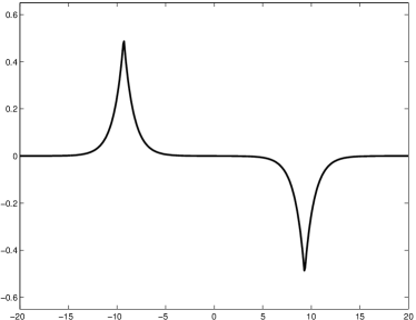
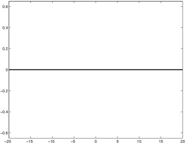
Figure 1. The peakon-antipeakon solution at times $0$ and $t_{0}$ for three different values of $\alpha$. (The curves coincide.)

Consider the initial data:

(5.1) $$u(0,x)=\begin{cases}\operatorname{sgn}(x)A(0)e^{-\left|x\right|},&\text{for $\left|x\right|>\gamma(0)$},\\ B(0)\sinh x,&\text{for $\left|x\right|\leq\gamma(0)$},\end{cases}$$

where we have introduced

(5.2) $$A(t)=\frac{E}{2}\sinh(\frac{E}{2}(t-t_{0})),\quad B(t)=E\sinh^{-1}(\frac{E}{2}(t-t_{0})),\quad\gamma(t)=\ln\cosh(\frac{E}{2}(t-t_{0})).$$

Here $t_{0}>0$ is a given time where the wave breaking will occur. For $t<t_{0}$ the function

(5.3) $$u(t,x)=\begin{cases}\operatorname{sgn}(x)A(t)e^{-\left|x\right|},&\text{for $\left|x\right|>\gamma(t)$},\\ B(t)\sinh x,&\text{for $\left|x\right|\leq\gamma(t)$},\end{cases}$$

will be the peakon-antipeakon solution of the Camassa–Holm equation (1.1) with $\kappa=0$ and $\rho$ identically zero, see [26, Thm. 4.1, Ex. 4.2 (ii)]. Define the two Radon measures by

(5.4) $$\mu(t)=\nu(t)=u_{x}^{2}(t,x)\,dx,\quad u_{x}(t,x)=\begin{cases}-A(t)e^{-\left|x\right|},&\text{for $\left|x\right|>\gamma(t)$},\\ B(t)\cosh x,&\text{for $\left|x\right|\leq\gamma(t)$}.\end{cases}$$

Observe that

(5.5) $$\int_{\mathbb{R}}(u^{2}(t,x)+u_{x}^{2}(t,x))\,dx=E^{2}\text{ for all $t<t_{0}$.}$$

At $t=t_{0}$ we see that $A(t_{0})=\gamma(t_{0})=0$, and thus $u(t_{0},x)=u_{x}(t_{0},x)=0$ almost everywhere, while $\mu(t),\nu(t)\to E^{2}\delta_{0}$ as $t\uparrow t_{0}$. Let namely $M\subset\mathbb{R}$ be a measurable set. Then

(5.6) $$\mu(t)(M)=\int_{M}u_{x}^{2}(t,x)\,dx\underset{t\uparrow t_{0}}{\to}\begin{cases}E^{2},&\text{for $0\in M$},\\ 0,&\text{for $0\not\in M$},\end{cases}$$

since $\gamma(t)\to 0$ and $u_{x}(t,x)\to 0$ ($x\neq 0$) as $t\uparrow t_{0}$, and

(5.7) $$\int_{-\gamma(t)}^{\gamma(t)}u_{x}^{2}(t,x)\,dx =B^{2}(t)\int_{-\gamma(t)}^{\gamma(t)}\cosh^{2}(x)\,dx$$

$$=B^{2}(t)\big{(}\gamma(t)+\frac{1}{2}\sinh(2\gamma(t))\big{)}\underset{t\uparrow t_{0}}{\to}E^{2}.$$

Next we turn to the Lagrangian variables, which are solutions of the following system of ordinary differential equations (cf. (2.19)) for $t<t_{0}$,

(5.8a) $$y_{t} =U,$$

(5.8b) $$U_{t} =-Q,$$

(5.8c) $$y_{t,\xi} =U_{\xi},$$

(5.8d) $$U_{t,\xi} =\frac{1}{2}h+(U^{2}-P)y_{\xi},$$

(5.8e) $$h_{t} =2(U^{2}-P)U_{\xi},$$

(5.8f) $$\bar{h}_{t} =h_{t},$$

where $P$ and $Q$ are given by (2.20) and (2.21), respectively. However, this system is difficult to solve directly, even in the case of a peakon-antipeakon solution. The initial data have to be judiciously chosen, and we will return to this shortly. Instead of solving (5.8) directly, we will determine the solution by using the connection between Eulerian and Lagrangian variables directly. The key relations are

(5.9) $$y_{t}=u\circ y,\quad U=u\circ y,\quad h=u_{x}^{2}\circ y\,y_{\xi}.$$

We have to determine the characteristics initially (here denoted by $\bar{y}_{0}$), given by (3.9a), that is, $\bar{y}_{0}(\xi)=\sup\left\{y\mid\nu((-\infty,y))+y<\xi\right\}$ (we write $\bar{y}_{0}$ rather than $y_{0}$ as we will modify it shortly). In this case, where the measure $\nu$ is absolutely continuous, we find that the characteristics is given by

(5.10) $$\int_{-\infty}^{\bar{y}_{0}(\xi)}u_{x}^{2}(0,x)dx+\bar{y}_{0}(\xi)=\xi,$$

which appears to be difficult to solve, even in this case. Fortunately, its derivative is straightforward:

(5.11) $$\bar{y}_{0}^{\prime}(\xi) =\frac{1}{1+u_{x}^{2}(0,\bar{y}_{0}(\xi))}$$

$$=\begin{cases}\big{(}1+A^{2}(0)e^{-\operatorname{sgn}(\xi)2\bar{y}_{0}(\xi)}\big{)}^{-1},&\text{for $\xi\not\in[\xi_{-},\xi_{+}]$},\\ \big{(}1+B^{2}(0)\cosh^{2}(\bar{y}_{0}(\xi))\big{)}^{-1},&\text{for $\xi\in[\xi_{-},\xi_{+}]$},\end{cases}$$

where we introduced $\xi_{\pm}$, the solution of $\bar{y}_{0}(\xi_{\pm})=\pm\gamma(0)$. For reasons that will become clear later, we will benefit from having characteristics that satisfy $y_{0}(\pm\gamma(0))=\pm\gamma(0)$, which is not automatically satisfied by (5.10). We use the freedom given to us by relabeling to modify $\bar{y}_{0}$. To that end define

(5.12) $$f(z)=\int_{-\infty}^{z}u_{x}^{2}(0,x)dx+z.$$

Then $f$ is a relabeling function in the sense of Definition 3.3. Observe that with this definition $\xi_{\pm}=f(\pm\gamma(0))$ and $f^{\prime}(z)=u_{x}^{2}(0,z)+1$. Introduce

(5.13) $$y_{0}(z)=\bar{y}_{0}(f(z)),$$

which implies

(5.14) $$y_{0}(\pm\gamma(0))=\bar{y}_{0}(f(\pm\gamma(0)))=\bar{y}_{0}(\xi_{\pm})=\pm\gamma(0).$$

Hence

(5.15) $$y_{0}^{\prime}(\xi) =\bar{y}^{\prime}_{0}\circ f(\xi)f^{\prime}(\xi)=1.$$

Thus the relabeled initial characteristics is simply $y_{0}(\xi)=\xi$. Clearly, we could have chosen this function immediately, and the above argument shows that one can always use the identity as the initial characteristics when the initial data contains no singular part. However, the above argument illustrates the possible use of relabeling.

The Lagrangian variables are then given, using (5.9) for $t<t_{0}$, by

(5.16) $$y(t,\xi) =\begin{cases}\xi+\operatorname{sgn}(\xi)\ln\big{(}1+(\cosh(\frac{E}{2}(t-t_{0}))-\cosh(\frac{E}{2}t_{0}))e^{-\left|\xi\right|}\big{)},&\text{for $\left|\xi\right|\geq\gamma(0)$},\\ 2\operatorname{artanh}\Big{(}\tanh(\frac{\xi}{2})\frac{\tanh^{2}(\frac{E}{4}(t-t_{0}))}{\tanh^{2}(-\frac{E}{4}t_{0})}\Big{)},&\text{for $\left|\xi\right|\leq\gamma(0)$},\end{cases}$$

$$U(t,\xi) =\begin{cases}\begin{matrix}\operatorname{sgn}(\xi)A(t)e^{-\left|\xi\right|}\\ \times\big{(}1+(\cosh(\frac{E}{2}(t-t_{0}))-\cosh(\frac{E}{2}t_{0}))e^{-\left|\xi\right|}\big{)}^{-1}\end{matrix},&\text{for $\left|\xi\right|\geq\gamma(0)$},\\ \begin{matrix}2B(t)\tanh(\frac{\xi}{2})\frac{\tanh^{2}(\frac{E}{4}(t-t_{0}))}{\tanh^{2}(-\frac{E}{4}t_{0})}\\ \times\big{(}1-\tanh^{2}(\frac{\xi}{2})\frac{\tanh^{4}(\frac{E}{4}(t-t_{0}))}{\tanh^{4}(-\frac{E}{4}t_{0})}\big{)}^{-1}\end{matrix},&\text{for $\left|\xi\right|\leq\gamma(0)$},\end{cases}$$

$$h(t,\xi) =\begin{cases}\begin{matrix}A(t)^{2}e^{-2\left|\xi\right|}\\ \times\big{(}1+(\cosh(\frac{E}{2}(t-t_{0}))-\cosh(\frac{E}{2}t_{0}))e^{-\left|\xi\right|}\big{)}^{-3}\end{matrix},&\text{for $\left|\xi\right|\geq\gamma(0)$},\\ \begin{matrix}B(t)^{2}\Big{(}1+\tanh^{2}(\frac{\xi}{2})\frac{\tanh^{4}(\frac{E}{4}(t-t_{0}))}{\tanh^{4}(-\frac{E}{4}t_{0})}\Big{)}^{2}\\ \times\Big{(}1-\tanh^{2}(\frac{\xi}{2})\frac{\tanh^{4}(\frac{E}{4}(t-t_{0}))}{\tanh^{4}(-\frac{E}{4}t_{0})}\Big{)}^{-3}\\ \times\cosh^{-2}(\frac{\xi}{2})\frac{\tanh^{2}(\frac{E}{4}(t-t_{0}))}{\tanh^{2}(-\frac{E}{4}t_{0})}\end{matrix},&\text{for $\left|\xi\right|\leq\gamma(0)$},\end{cases}$$

$$\bar{h}(t,\xi) =h(t,\xi),$$

$$P(t,\xi) =\frac{1}{4}\int_{\mathbb{R}}e^{-|y(t,\xi)-y(t,\eta)|}(2U^{2}y_{\xi}+h)(t,\eta)d\eta,$$

$$Q(t,\xi) =-\frac{1}{4}\int_{\mathbb{R}}\operatorname{sgn}{(\xi-\eta)}e^{-|y(t,\xi)-y(t,\eta)|}(2U^{2}y_{\xi}+h)(t,\eta)d\eta.$$

With the choice of initial characteristics we obtain

(5.17) $$y(t,\pm\gamma(0))=\pm\gamma(t),$$

and hence at the peaks

(5.18) $$U(t,\pm\gamma(0))=u(t,\pm\gamma(t))=\pm\frac{E}{2}\tanh\big{(}\frac{E}{2}(t-t_{0})\big{)}.$$

As expected

(5.19) $$\tau(\xi)=\begin{cases}\infty,&\text{for $\left|\xi\right|\geq\gamma(0)$},\\ t_{0},&\text{for $\left|\xi\right|<\gamma(0)$}.\end{cases}$$

The important quantity is the first time there is wave breaking. By construction

(5.20) $$t_{0}=\inf_{\xi}\tau(\xi).$$

Next we consider the limits of these variables as $t\uparrow t_{0}$:

(5.21) $$\lim_{t\uparrow t_{0}}y(t,\xi) =\begin{cases}\xi+\operatorname{sgn}(\xi)\ln\big{(}1+(1-\cosh(\frac{E}{2})t_{0})e^{-\left|\xi\right|}\big{)},&\text{for $\left|\xi\right|\geq\gamma(0)$},\\ 0,&\text{for $\left|\xi\right|<\gamma(0)$},\end{cases}$$

$$\lim_{t\uparrow t_{0}}U(t,\xi) =0,$$

$$\lim_{t\uparrow t_{0}}h(t,\xi) =\begin{cases}0,&\text{for $\left|\xi\right|\geq\gamma(0)$},\\ \frac{E^{2}}{4}\cosh^{-2}(\frac{\xi}{2})\tanh^{-2}(-\frac{E}{4}t_{0}),&\text{for $\left|\xi\right|\leq\gamma(0)$},\end{cases}$$

$$\lim_{t\uparrow t_{0}}P(t,\xi) =\begin{cases}\frac{E^{2}}{4}(1+(1-\cosh(\frac{E}{2}t_{0}))e^{-\left|\xi\right|})^{-1}e^{-\left|\xi\right|},&\text{for $\left|\xi\right|\geq\gamma(0)$},\\ \frac{E^{2}}{4},&\text{for $\left|\xi\right|\leq\gamma(0)$},\end{cases}$$

$$\lim_{t\uparrow t_{0}}Q(t,\xi) =-\begin{cases}\operatorname{sgn}(\xi)\frac{E^{2}}{4}(1+(1-\cosh(\frac{E}{2}t_{0}))e^{-\left|\xi\right|})^{-1}e^{-\left|\xi\right|},&\text{for $\left|\xi\right|\geq\gamma(0)$},\\ \frac{E^{2}}{4}\tanh^{-2}(-\frac{E}{4}t_{0})\tanh(\frac{\xi}{2}),&\text{for $\left|\xi\right|\leq\gamma(0)$}.\end{cases}$$

At $t=t_{0}$ we introduce the parameter $\alpha\in[0,1]$, and define

(5.22) $$\bar{h}(t_{0},\xi)=(1-\alpha)\lim_{t\uparrow t_{0}}h(t,\xi),\quad h(t_{0},\xi)=\lim_{t\uparrow t_{0}}h(t,\xi).$$

This implies that in Eulerian variables

(5.23) $$u(t_{0},x)=0,\quad\mu(t_{0})=(1-\alpha)E^{2}\delta_{0},\quad\text{and}\quad\nu(t_{0})=E^{2}\delta_{0},$$

using the definitions (3.24b), namely $\mu=y_{\#}(\bar{h}(\xi)\,d\xi)$, and (3.24c), that is, $\nu=y_{\#}(h(\xi)\,d\xi)$.

We will show that for $t>t_{0}$ the solution coincides with the peakon-antipeakon solution with the energy $E$ replaced by

(5.24) $$\tilde{E}=\sqrt{1-\alpha}\,E.$$

For $t>t_{0}$ the Lagrangian system reads (cf. (2.19))

(5.25a) $$y_{t} =U,$$

(5.25b) $$U_{t} =-Q,$$

(5.25c) $$y_{t,\xi} =U_{\xi},$$

(5.25d) $$U_{t,\xi} =\frac{1}{2}\bar{h}+(U^{2}-P)y_{\xi},$$

(5.25e) $$h_{t} =2(U^{2}-P)U_{\xi},$$

(5.25f) $$\bar{h}_{t} =h_{t},$$

where $P$ and $Q$ are given by (2.20) and (2.21), respectively.

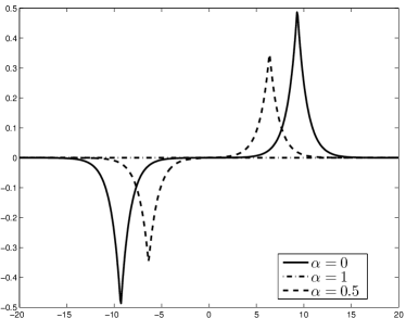
Figure 2. The peakon-antipeakon solution at times $0$ and $t>t_{0}$ for three different values of $\alpha$.

In the fully dissipative case with $\alpha=1$, we get $\bar{h}(t_{0})=0$, but also $(U^{2}-P)(t_{0})=U_{\xi}(t_{0})=Q(t_{0})=0$, and hence we have for $t>t_{0}$:

(5.26) $$y(t,\xi) =y(t_{0},\xi),$$

$$U(t,\xi) =0,$$

$$h(t,\xi) =h(t_{0},\xi),$$

$$\bar{h}(t,\xi) =0.$$

This implies that in Eulerian variables

(5.27) $$u(t,x)=0,\quad\mu(t)=0,\quad\nu(t)=E^{2}\delta_{0},\qquad t>t_{0}.$$

In the general case $\alpha\in[0,1)$, it is difficult, as it was for $t<t_{0}$, to solve the system (5.25) explicitly. However, we proceed as follows. Given (5.23), we use (3.9a), denoting the characteristics by $\tilde{y}(t_{0})$, to determine the new initial characteristics. We find

(5.28) $$\tilde{y}(t_{0},\xi)=\begin{cases}\xi,&\text{for $\xi\leq 0$},\\ 0,&\text{for $0\leq\xi<\tilde{E}^{2}$},\\ \xi-\tilde{E}^{2},&\text{for $\xi\geq\tilde{E}^{2}$}.\end{cases}$$

Note that this function is related by relabeling to the characteristics we already have at $t=t_{0}$, given by (5.21), namely

(5.29) $$y(t_{0},\xi)=\begin{cases}\xi+\operatorname{sgn}(\xi)\ln\big{(}1+(1-\cosh(\frac{E}{2}t_{0}))e^{-\left|\xi\right|}\big{)},&\text{for $\left|\xi\right|\geq\gamma(0)$},\\ 0,&\text{for $\left|\xi\right|<\gamma(0)$}.\end{cases}$$

To that end define

(5.30) $$g(\xi) =y(t_{0},\xi)+\bar{H}(t_{0},\xi)=y(t_{0},\xi)+\int_{-\infty}^{\xi}\bar{h}(t_{0},\eta)\,d\eta$$

$$=\begin{cases}\xi-\ln\big{(}1+(1-\cosh(\frac{E}{2}t_{0}))e^{\xi}\big{)},&\text{for $\xi\leq-\gamma(0)$},\\ \frac{\tilde{E}^{2}}{2}\big{(}\tanh^{-2}(-\frac{E}{4}t_{0})\tanh(\frac{\xi}{2})+1\big{)},&\text{for $-\gamma(0)\leq\xi<\gamma(0)$},\\ \xi+\tilde{E}^{2}+\ln\big{(}1+(1-\cosh(\frac{E}{2}t_{0}))e^{-\xi}\big{)},&\text{for $\xi\geq\gamma(0)$}.\end{cases}$$

Observe that $g$ is a monotonically increasing relabeling function that satisfies

(5.31) $$\lim_{\xi\to-\gamma(0)}g(\xi)=0,\qquad\lim_{\xi\to\gamma(0)}g(\xi)=\tilde{E}^{2},$$

and thus

(5.32) $$y(t_{0},\xi)=\tilde{y}(t_{0},g(\xi)).$$

We are now given initial data $y(t_{0})$, as well as $U(t_{0})=0$ and $h(t_{0})$. We claim that the solution, in Eulerian variables, is

(5.33) $$u(t,x)=\begin{cases}\operatorname{sgn}(x)\tilde{A}(t)e^{-\left|x\right|},&\text{for $\left|x\right|>\tilde{\gamma}(t)$},\\ \tilde{B}(t)\sinh x,&\text{for $\left|x\right|\leq\tilde{\gamma}(t)$},\end{cases}\qquad t>t_{0},$$

where

(5.34) $$\tilde{A}(t)=\frac{\tilde{E}}{2}\sinh(\frac{\tilde{E}}{2}(t-t_{0})),\quad\tilde{B}(t)=\tilde{E}\sinh^{-1}(\frac{\tilde{E}}{2}(t-t_{0})),\quad\tilde{\gamma}(t)=\ln\cosh(\frac{\tilde{E}}{2}(t-t_{0})).$$

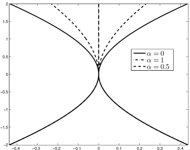
Figure 3. The characteristics $y(t,\pm\gamma(0))$ describing the location of the peaks of the peak-antipeakon solution for three different values of $\alpha$.

To determine the characteristics we solve the equation $y_{t}=u\circ y$. We provide some details. Consider first the case $\xi\leq-\gamma(0)$. Integrating we find

(5.35) $$e^{-y(t,\xi)}-e^{-y(t_{0},\xi)}=\cosh(\frac{\tilde{E}}{2}(t-t_{0}))-1.$$

Inserting the expression (5.29), we find

(5.36) $$y(t,\xi)=\xi-\ln\big{(}1+(\cosh(\frac{\tilde{E}}{2}(t-t_{0}))-\cosh(\frac{E}{2}t_{0}))e^{\xi}\big{)}.$$

A similar calculation determines the case $\xi\geq\gamma(0)$. Assume now that $-\gamma(0)\leq\xi\leq\gamma(0)$. Integrating the equation we find, for any small, positive $\varepsilon$, that

(5.37) $$\ln\tanh(\frac{1}{2}y(t,\xi))-\ln\tanh(\frac{1}{2}y(t_{0}+\varepsilon,\xi))\\ =2\big{(}\ln\tanh(\frac{\tilde{E}}{4}(t-t_{0}))-\ln\tanh(\frac{\tilde{E}}{4}\varepsilon)\big{)},$$

which rewrites to

(5.38) $$y(t,\xi)=2\operatorname{artanh}\Big{(}\tanh(\frac{1}{2}y(t_{0}+\varepsilon,\xi))\frac{\tanh^{2}(\frac{\tilde{E}}{4}(t-t_{0}))}{\tanh^{2}(\frac{\tilde{E}}{4}\varepsilon)}\Big{)}.$$

Taking $\varepsilon\downarrow 0$ we find that

(5.39) $$y(t,\xi)=2\operatorname{artanh}\Big{(}\tanh(\frac{\xi}{2})\frac{\tanh^{2}(\frac{\tilde{E}}{4}(t-t_{0}))}{\tanh^{2}(-\frac{E}{4}t_{0})}\Big{)}.$$

Note that this limit is rather delicate. As it involves repeated use of L’Hôpital’s rule, one has to invoke the equations (5.25) in order to compute the limit. We can now determine the remaining Lagrangian quantities:

(5.40) $$y(t,\xi) =\begin{cases}\xi+\operatorname{sgn}(\xi)\ln\big{(}1+(\cosh(\frac{\tilde{E}}{2}(t-t_{0}))-\cosh(\frac{E}{2}t_{0}))e^{-\left|\xi\right|}\big{)},&\text{for $\left|\xi\right|\geq\gamma(0)$},\\ 2\operatorname{artanh}\Big{(}\tanh(\frac{\xi}{2})\frac{\tanh^{2}(\frac{\tilde{E}}{4}(t-t_{0}))}{\tanh^{2}(-\frac{E}{4}t_{0})}\Big{)},&\text{for $\left|\xi\right|\leq\gamma(0)$},\end{cases}$$

$$U(t,\xi) =\begin{cases}\begin{matrix}\operatorname{sgn}(\xi)\tilde{A}(t)e^{-\left|\xi\right|}\\ \times\big{(}1+(\cosh(\frac{\tilde{E}}{2}(t-t_{0}))-\cosh(\frac{E}{2}t_{0}))e^{-\left|\xi\right|}\big{)}^{-1}\end{matrix},&\text{for $\left|\xi\right|\geq\gamma(0)$},\\ \begin{matrix}2\tilde{B}(t)\tanh(\frac{\xi}{2})\frac{\tanh^{2}(\frac{\tilde{E}}{4}(t-t_{0}))}{\tanh^{2}(-\frac{E}{4}t_{0})}\\ \times\big{(}1-\tanh^{2}(\frac{\xi}{2})\frac{\tanh^{4}(\frac{\tilde{E}}{4}(t-t_{0}))}{\tanh^{4}(-\frac{E}{4}t_{0})}\big{)}^{-1}\end{matrix},&\text{for $\left|\xi\right|\leq\gamma(0)$},\end{cases}$$

$$\bar{h}(t,\xi) =\begin{cases}\begin{matrix}\tilde{A}(t)^{2}e^{-2\left|\xi\right|}\\ \times\big{(}1+(\cosh(\frac{\tilde{E}}{2}(t-t_{0}))-\cosh(\frac{E}{2}t_{0}))e^{-\left|\xi\right|}\big{)}^{-3}\end{matrix},&\text{for $\left|\xi\right|\geq\gamma(0)$},\\ \begin{matrix}\tilde{B}(t)^{2}\Big{(}1+\tanh^{2}(\frac{\xi}{2})\frac{\tanh^{4}(\frac{\tilde{E}}{4}(t-t_{0}))}{\tanh^{4}(-\frac{E}{4}t_{0})}\Big{)}^{2}\\ \times\Big{(}1-\tanh^{2}(\frac{\xi}{2})\frac{\tanh^{4}(\frac{\tilde{E}}{4}(t-t_{0}))}{\tanh^{4}(-\frac{E}{4}t_{0})}\Big{)}^{-3}\\ \times\cosh^{-2}(\frac{\xi}{2})\frac{\tanh^{2}(\frac{\tilde{E}}{4}(t-t_{0}))}{\tanh^{2}(-\frac{E}{4}t_{0})}\end{matrix},&\text{for $\left|\xi\right|\leq\gamma(0)$},\end{cases}$$

$$h(t,\xi) =\begin{cases}\bar{h}(t,\xi),&\text{for $\left|\xi\right|\geq\gamma(0)$},\\ \bar{h}(t,\xi)+\alpha\frac{E^{2}}{4}\cosh^{-2}\big{(}\frac{\xi}{2}\big{)}\tanh^{-2}\big{(}-\frac{E}{4}t_{0}\big{)},&\text{for $\left|\xi\right|<\gamma(0)$},\end{cases}$$

$$P(t,\xi) =\frac{1}{4}\int_{\mathbb{R}}e^{-|y(t,\xi)-y(t,\eta)|}(2U^{2}y_{\xi}+\bar{h})(t,\eta)d\eta,$$

$$Q(t,\xi) =-\frac{1}{4}\int_{\mathbb{R}}\operatorname{sgn}{(\xi-\eta)}e^{-|y(t,\xi)-y(t,\eta)|}(2U^{2}y_{\xi}+\bar{h})(t,\eta)d\eta.$$

To complete the calculation of the Eulerian variables, we use the definitions (3.24b) and (3.24c) to determine the measures. First we find

(5.41) $$\mu(t)=u_{x}^{2}(t,x)\,dx,\quad t>t_{0}.$$

To determine $\nu(t)$ we write $h=\bar{h}+l_{1}$ (see (2.18)) with $\bar{h}=u_{x}^{2}\circ yy_{\xi}$. We want to determine a function $l$ such that $l_{1}=l\circ yy_{\xi}$, which implies $\nu=(\bar{h}+l)dx$. From (5.40) we see that $l_{1}(t,\xi)=0$ for $\left|\xi\right|\geq\gamma(0)$. For $\left|\xi\right|<\gamma(0)$ we first observe from (5.40) that

$$y_{\xi}(t,\xi) =\Big{(}1-\big{(}\tanh(\frac{\xi}{2})\frac{\tanh^{2}(\frac{\tilde{E}}{4}(t-t_{0}))}{\tanh^{2}(-\frac{E}{4}t_{0})}\big{)}^{2}\Big{)}^{-1}\cosh^{-2}(\frac{\xi}{2})\frac{\tanh^{2}(\frac{\tilde{E}}{4}(t-t_{0}))}{\tanh^{2}(-\frac{E}{4}t_{0})}$$

$$=\big{(}1-\tanh^{2}(\frac{y(t,\xi)}{2})\big{)}^{-1}\cosh^{-2}(\frac{\xi}{2})\frac{\tanh^{2}(\frac{\tilde{E}}{4}(t-t_{0}))}{\tanh^{2}(-\frac{E}{4}t_{0})},$$

using

$$\tanh(\frac{y(t,\xi)}{2})=\tanh(\frac{\xi}{2})\frac{\tanh^{2}(\frac{\tilde{E}}{4}(t-t_{0}))}{\tanh^{2}(-\frac{E}{4}t_{0})}.$$

Thus for $\left|\xi\right|<\gamma(0)$

$$l(t,y(t,\xi))=\frac{l_{1}(t,\xi)}{y_{\xi}(t,\xi)} =\alpha\frac{E^{2}}{4}\frac{\big{(}1-\tanh^{2}(\frac{y(t,\xi)}{2})\big{)}\cosh^{2}(\frac{\xi}{2})\tanh^{2}(-\frac{E}{4}t_{0})}{\cosh^{2}\big{(}\frac{\xi}{2}\big{)}\tanh^{2}(-\frac{E}{4}t_{0})\tanh^{2}(\frac{\tilde{E}}{4}(t-t_{0}))}$$

$$=\alpha\frac{E^{2}}{4}\big{(}1-\tanh^{2}(\frac{y(t,\xi)}{2})\big{)}\tanh^{-2}(\frac{\tilde{E}}{4}(t-t_{0})),$$

thus we infer that

$$l(t,x)=\begin{cases}0,&\text{for $\left|x\right|\geq\tilde{\gamma}(t)$},\\ \alpha\frac{E^{2}}{4}\big{(}1-\tanh^{2}(\frac{x}{2})\big{)}\tanh^{-2}(\frac{\tilde{E}}{4}(t-t_{0})),&\text{for $\left|x\right|\leq\tilde{\gamma}(t)$}.\end{cases}$$

Finally, we get the following expression

(5.42) $$\nu(t)=\begin{cases}u_{x}^{2}(t,x)\,dx,&\text{for $\left|x\right|\geq\tilde{\gamma}(t)$},\\ \Big{(}u_{x}^{2}(t,x)+\alpha\frac{E^{2}}{4}\tanh^{-2}\big{(}\frac{\tilde{E}}{4}(t-t_{0})\big{)}\big{(}1-\tanh^{2}\big{(}\frac{x}{2}\big{)}\big{)}\Big{)}\,dx,&\text{for $\left|x\right|\leq\tilde{\gamma}(t)$},\end{cases}$$

for $t>t_{0}$.

References

- [1] L. Ambrosio, N. Fusco, and D. Pallara. Functions of Bounded Variation and Free Discontinuity Problems. Clarendon Press, New York, 2000.
- [2] H. Aratyn, J. F. Gomes, and A. H. Zimerman. On a negative flow of the AKNS hierarchy and its relation to a two-component Camassa–Holm equation. Symmetry, Integrability and Geometry: Methods and Applications, vol. 2, Paper 070, 12 pages, 2006.
- [3] R. Beals, D. Sattinger, and J. Szmigielski. Peakon-antipeakon interaction. J. Nonlinear Math. Phys. 8:23–27, 2001.
- [4] A. Bressan and A. Constantin. Global conservative solutions of the Camassa–Holm equation. Arch. Ration. Mech. Anal., 183:215–239, 2007.
- [5] A. Bressan and A. Constantin. Global dissipative solutions of the Camassa–Holm equation. Analysis and Applications, 5:1–27, 2007.
- [6] A. Bressan, H. Holden, and X. Raynaud. Lipschitz metric for the Hunter–Saxton equation. J. Math. Pures Appl., 94:68–92, 2010.
- [7] R. Camassa and D. D. Holm. An integrable shallow water equation with peaked solitons. Phys. Rev. Lett., 71(11):1661–1664, 1993.
- [8] M. Chen, S.-Q. Liu, and Y. Zhang. A two-component generalization of the Camassa-Holm equation and its solutions. Lett. Math. Phys. 75:1–15, 2006.
- [9] R. M. Chen and Y. Liu. Wave breaking and global existence for a generalized two-component Camassa–Holm system. Inter. Math Research Notices, Article ID rnq118, 36 pages, 2010.
- [10] A. Constantin and J. Escher. Wave breaking for nonlinear nonlocal shallow water equations. Acta Math., 181:229–243, 1998.
- [11] A. Constantin and R. I. Ivanov. On an integrable two-component Camassa–Holm shallow water system. Phys. Lett. A 372:7129–7132, 2008.
- [12] J. Escher, O. Lechtenfeld, and Z. Yin. Well-posedness and blow-up phenomena for the 2-component Camassa–Holm equation. Discrete Contin. Dyn. Syst., 19(3):493–513, 2007.
- [13] Y. Fu and C. Qu. Well posedness and blow-up solution for a new coupled Camassa–Holm equations with peakons. J. Math. Phys., 50:012906, 2009.
- [14] K. Grunert, H. Holden, and X. Raynaud. Global conservative solutions of the Camassa–Holm equation for initial data with nonvanishing asymptotics. Discrete Cont. Dyn. Syst., Series A, 32:4209–4277, 2012.
- [15] K. Grunert, H. Holden, and X. Raynaud. Global solutions for the two-component Camassa–Holm system. Comm. Partial Differential Equations, 37:2245–2271, 2012.
- [16] K. Grunert, H. Holden, and X. Raynaud. Lipschitz metric for the Camassa–Holm equation on the line. Discrete Contin. Dyn. Syst. 33:2809–2827, 2013.
- [17] K. Grunert, H. Holden, and X. Raynaud. Periodic conservative solutions for the two-component Camassa–Holm system. In Spectral Analysis, Differential Equations and Mathematical Physics. A Festschrift for Fritz Gesztesy on the Occasion of his 60th Birthday (eds. H. Holden, B. Simon, and G. Teschl) Amer. Math. Soc., pp. 165–182, 2013.
- [18] K. Grunert, H. Holden, and X. Raynaud. Global dissipative solutions of the two-component Camassa–Holm system for initial data with nonvanishing asymptotics. Nonlinear Anal. Real World Appl. 17:203–244, 2014.
- [19] C. Guan, K. H. Karlsen, and Z. Yin. Well-posedness and blow-up phenomenal for a modified two-component Camassa–Holm equation. In: Nonlinear Partial Differential Equations and Hyperbolic Wave Phenomena (eds. H. Holden and K. H. Karlsen), Amer. Math. Soc., Contemporary Mathematics, vol. 526, pp. 199–220, 2010.
- [20] C. Guan and Z. Yin. Global existence and blow-up phenomena for an integrable two-component Camassa–Holm water system. J. Differential Equations, 248:2003–2014, 2010.
- [21] C. Guan and Z. Yin. Global weak solutions for a modified two-component Camassa–Holm equation. Ann. I. H. Poincaré – AN 28:623–641, 2011.
- [22] C. Guan and Z. Yin. Global weak solutions for a two-component Camassa–Holm shallow water system. J. Func. Anal. 260:1132–1154, 2011.
- [23] G. Gui and Y. Liu. On the Cauchy problem for the two-component Camassa–Holm system. Math Z, 268:45–66, 2011.
- [24] G. Gui and Y. Liu. On the global existence and wave breaking criteria for the two-component Camassa–Holm system. J. Func. Anal., 258:4251–4278, 2010.
- [25] Z. Guo and Y. Zhou. On solutions to a two-component generalized Camassa–Holm equation. Studies Appl. Math., 124:307–322, 2010.
- [26] H. Holden and X. Raynaud. Global conservative multipeakon solutions of the Camassa–Holm equation. J. Hyperbolic Differ. Equ., 4:39–64, 2007.
- [27] H. Holden and X. Raynaud. Global conservative solutions of the Camassa–Holm equation — a Lagrangian point of view. Comm. Partial Differential Equations, 32:1511–1549, 2007.
- [28] H. Holden and X. Raynaud. Global dissipative multipeakon solutions for the Camassa–Holm equation Commun. in Partial Differential Equations, 33 (2008) 2040–2063.
- [29] H. Holden and X. Raynaud. Dissipative solutions of the Camassa–Holm equation. Discrete Cont. Dyn. Syst., 24:1047–1112, 2009.
- [30] D. D. Holm, L. Ó. Náraigh, and C. Tronci. Singular solutions of a modified two-component Camassa–Holm equation. Phys. Rev. E 79 016601, 2009.
- [31] Q. Hu and Z. Yin. Well-posedness and blow-up phenomena for a periodic two-component Camassa–Holm equation. Proc. Roy. Soc. Edinburgh 141A 93–107, 2011.
- [32] R. I. Ivanov. Extended Camassa–Holm hierarchy and conserved quantities. Z. Naturforschung 61A:133–138, 2006.
- [33] P. A. Kuz’min. Two-component generalizations of the Camassa–Holm equation. Math. Notes, 81:130–134, 2007.
- [34] L. Tian, Y. Wang, and J. Zhou. Global conservative and dissipative solutions of a coupled Camassa–Holm equations. J. Math. Phys. 52 063702, 2011.
- [35] P. J. Olver and P. Rosenau. Tri-hamiltonian duality between solitons and solitary-wave solutions having compact support. Phys. Rev. B, 53(2):1900–1906, 1996.
- [36] E. Wahlén. The interaction of peakons and antipeakons. Dyn. Contin. Discrete Impuls. Syst. Ser. A. 13:465-472, 2006.
- [37] Y. Wang, J. Huang, and L. Chen. Global conservative solutions of the two-component Camassa–Holm shallow water system. Int. J. Nonlin. Science, 9:379–384, 2009.