i-PI: A Python interface for ab initio path integral molecular dynamics simulations

Abstract

Recent developments in path integral methodology have significantly reduced the computational expense of including quantum mechanical effects in the nuclear motion in ab initio molecular dynamics simulations. However, the implementation of these developments requires a considerable programming effort, which has hindered their adoption. Here we describe i-PI, an interface written in Python that has been designed to minimise the effort required to bring state-of-the-art path integral techniques to an electronic structure program. While it is best suited to first principles calculations and path integral molecular dynamics, i-PI can also be used to perform classical molecular dynamics simulations, and can just as easily be interfaced with an empirical forcefield code. To give just one example of the many potential applications of the interface, we use it in conjunction with the CP2K electronic structure package to showcase the importance of nuclear quantum effects in high pressure water.

1 Introduction

Molecular dynamics simulations are becoming increasingly capable not only of assisting the interpretation of experiments, but also of predicting the properties and the behaviour of new materials and compounds [1]. Besides the increase in available computer power, these developments have been made possible by an increasingly accurate treatment of the interactions between the atoms, in particular by an explicit treatment of the electronic structure problem [2, 3]. However, as the methods that are used to treat the quantum nature of the electrons improve, it becomes increasingly clear that in the presence of light atoms, such as hydrogen or lithium, the error due to approximating the nuclei as classical particles is at least as large as the errors due to the approximate modelling of the electrons. The importance of nuclear quantum effects (NQEs) is evident from the fact that the zero-point energy associated with a typical O–H stretching mode is in excess of 200 meV. This has significant implications: for example, one can show by extrapolating the experimental values for isotopically pure light, heavy and tritiated water that a hypothetical liquid with classical nuclei would have a 50% higher heat capacity than H₂O and a pH of about 8.5.

Within the Born-Oppenheimer approximation, NQEs can be modelled using the imaginary time path integral formalism [4, 5, 6, 7]. This formalism maps the quantum mechanical partition function for a set of distinguishable nuclei onto the classical partition function of a so-called ring polymer, composed of $n$ replicas (beads) of the physical system connected by harmonic springs. The number of replicas needed to achieve a converged result is typically a small multiple of $\beta\hbar\omega_{\rm max}$, where $\beta$ is the inverse temperature and $\omega_{\rm max}$ is the largest vibrational frequency in the system. For the archetypical case of room-temperature liquid water, most properties are reasonably well converged with $n=32$ – making the path integral simulation 32 times more expensive than a classical simulation.

As a consequence of this large overhead, NQEs were for many years only rarely considered in the context of ab initio molecular dynamics [8, 9, 10]. However, with the advent of massively parallel computers, including these effects has become somewhat more affordable [11, 12], and their simulation has also been facilitated by new methodological developments. In particular, it has recently been realised that an approximate modelling of NQEs can be obtained by applying a coloured (correlated)-noise Langevin equation thermostat to classical molecular dynamics [13, 14, 15]. Moreover, this idea can be turned into a systematically convergent, accurate method [16, 17] by combining coloured noise with path integral molecular dynamics (PIMD). To give an example, the PIGLET method [17] makes it possible to treat NQEs in liquid water at 300 K with as few as 6 beads, which promises to make accurate ab initio PIMD calculations almost routine.

Unfortunately, most ab initio electronic structure codes only contain rudimentary implementations of PIMD, if any at all. We have developed i-PI in order to reduce the effort of introducing the latest PIMD developments into electronic structure codes, so as to make them readily available to a broader community. The framework we have adopted is a server-client model, in which i-PI acts as a server passing atomic coordinates to (multiple instances of) an electronic structure client program, and receiving the energy and forces in return. This allows all of the PIMD machinery to be confined to the Python server side, and minimises the modifications that have to be made to the electronic structure code.

2 Program overview

i-PI has been developed with the awareness that the cost of an ab initio PIMD simulation will be dominated by the electronic structure problem, and with a few clear goals:

• to minimise the effort required to modify the client ab initio electronic structure code,

• to include no feature specific to a particular client code,

• to be modular, simple to extend and with a structure that reflects the underlying physics,

• to be efficient, but never at the cost of clarity.

In order to acheive these goals we have chosen the Python programming language, and a client-server model in which i-PI acts as the server, dealing exclusively with evolving the nuclear degrees of freedom according to the equations of motion. The evaluation of the forces, the potential and the virial is delegated to one or more instances of the client code (see Figure 1). i-PI maintains a list of active clients, to which it dispatches the positions of the nuclei and from which it collects the forces and energy as soon as they have been computed. The communication is kept to a minimum, not so much for its impact on performance, as for the fact that exchanging more information would require a more substantial implementation effort on the client side. All the details of the force evaluation – such as the parameters of the electronic structure calculation – are left to the input of the external code: i-PI only sends the dimensions of the simulation box ($\mathbf{h}$) and the coordinates of the nuclei ($\mathbf{x}$), and expects the atomic species to be stored internally by the client code in the same order they are in the i-PI input. The client code computes and returns the ionic forces ($\mathbf{f}$), electronic energy ($U$) and stress tensor ($\boldsymbol{\sigma}$), possibly supplemented by a string that contains any further information on the electronic structure (e.g. the dipole moment, the partial charges of the atoms, etc.) that might be required for post-processing; i-PI simply outputs this string verbatim.

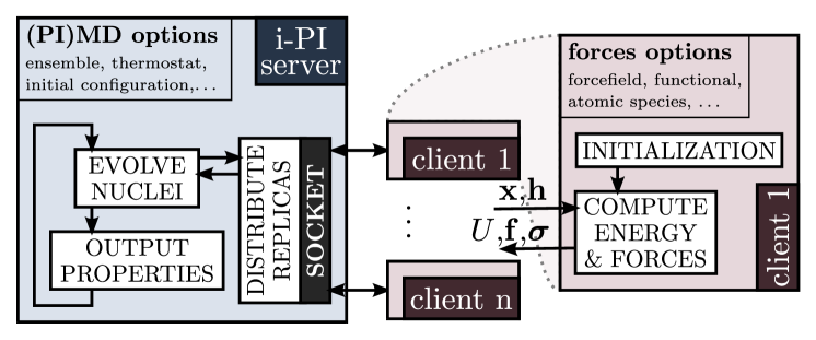
Figure 1: Schematic overview of the client-server model underlying i-PI. The communication is kept to a minimum, and so are the modifications that need to be made to adapt an existing electronic structure code to act as the client. The client is not restarted between successive force evaluations, so that the overhead associated with initialisation is avoided.

The client-server communication is implemented using sockets. If desired, i-PI can communicate with the clients across the internet, realising a rudimentary distributed computing paradigm. If one wishes to reduce the communication overhead – e.g. if one wants to use i-PI with an empirical forcefield driver – local UNIX-domain sockets can be used. It would also be easy to implement different communication methods, e.g. via inter-process MPI or writing to disk.

Instances of the patched ab initio code can register themselves dynamically, and i-PI keeps track of the active clients so that the forces on multiple path integral replicas can be evaluated at once. The trivial layer of parallelism over the beads can therefore be fully exploited. We would recommend implementing the communication code into the client software in a way that mimics one of the existing procedures that update nuclear positions, as is done in molecular dynamics, geometry optimisation, etc. The electronic structure infrastructure only has to be initialised once, before the client connects to the i-PI server and waits to receive a set of atomic coordinates. It then performs an electronic structure calculation, returns the energy, forces and stress tensor to the server, and waits for the next set of coordinates. The converged density/wavefunction from the previous step can be re-used as the starting point for the next, which is advantageous because in all probability this will correspond to a very similar atomic configuration. This makes our approach superior to a scripting approach in which the client code is re-launched with a new input for each atomic configuration. In order to fully take advantage of the density/wavefunction extrapolation techniques implemented in many modern electronic structure codes, i-PI will always try to dispatch the same replica to a given instance of the client, to ensure that a smooth sequence of configurations is provided to each client from one time step to the next.

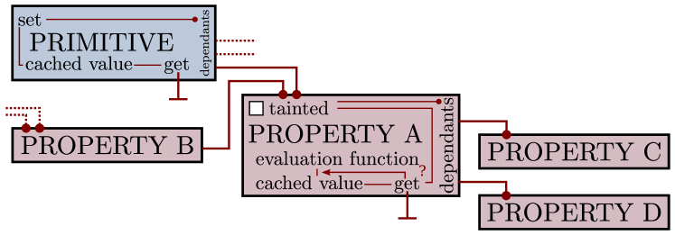
Figure 2: Schematic overview of the functioning of the depend class used as the base for properties and physical quantities in i-PI. A few “primitive” quantities – such as atomic positions or momenta – can be modified directly. For most properties, one defines a function that can compute their value based on the values of other properties. Whenever one property is modified, all the quantities that depend on it are marked as tainted, so that – when the value of one of the properties is used, the function can be invoked and the updated value can be obtained and cached. If the same quantity is requested again and it has not been marked as tainted in the mean time, the cached value is returned.

To make the internal coding of i-PI as transparent and as close to the physics of the problem as possible, we have introduced a dedicated Python class to represent physical quantities – such as the atomic coordinates, the momenta, the kinetic energy, etc. Instances of this class can be used simply as variables containing the value of the quantity they represent. However, they also contain information on how each quantity depends on others, and how it can be computed from its dependencies (see Figure 2). Derived quantities are computed automatically when requested, and their value is cached for future reference. If the same quantity is needed again, the cached value will be used, avoiding the overhead of re-computing it. If however one of the quantities it depends on has been modified, it will be re-evaluated automatically. This mechanism of dependency detection and value caching considerably de-clutters the code, since one does not need to keep track of when quantities need to be recomputed.

The input for i-PI consists in a xml file, containing a number of tags and options that specify the details of the simulation. The list of available options are described in detail in the manual. i-PI can dump the full state of the simulation as checkpoint files, that can be used to seamlessly re-start a simulation and that have the same format of an input file, so it is easy to modify some of the options, if desired.

3 Program features

Integrating the PIMD equations of motion involves a number of technicalities. Fortunately, these can be kept to a minimum by using stochastic thermostatting [18] – which avoids the complication of integrating Nosé-Hoover chain thermostats – and by formulating the time evolution using a symmetric Trotter splitting algorithm [19]. This is the approach we have adopted in the i-PI program.

The program implements the most recent developments in path integral and colored-noise molecular dynamics, including the following:

• molecular dynamics and PIMD in the NVE, NVT and NPT ensembles, with the high-frequency internal vibrations of the path propagated in the normal-mode representation [18];

• ring polymer contraction [20, 21], implemented by exposing multiple socket interfaces to deal separately with short and long-range components of the potential energy;

• efficient stochastic velocity rescaling [22] and path integral Langevin equation thermostats [18];

• various generalized Langevin equation (GLE) thermostats, including the optimal sampling [23, 24], quantum  [14], and $\delta$ [25] thermostats, the parameters for which can be downloaded from an on-line repository [26];

• mixed path integral–generalized Langevin equation techniques for accelerated convergence, including both PI+GLE [16] and the more recent and effective version PIGLET [17];

• all the standard estimators for structural properties, the quantum kinetic energy, pressure, etc.;

• more sophisticated estimators such as the scaled-coordinate heat capacity estimator [27], estimators to obtain isotope fractionation free energies by re-weighting a simulation of the most abundant isotope [28], and a displaced-path estimator for the particle momentum distribution [29];

• the infrastructure that is needed to perform ring polymer molecular dynamics (RPMD) [30, 31] and centroid molecular dynamics (CMD) [32, 33] approximate quantum dynamics calculations.

4 Constant-pressure path integral molecular dynamics

Most of the techniques listed above have been discussed in detail elsewhere. However, our implementation of PIMD in the NPT ensemble has not been described before now. The approach we have adopted for this is a relatively straightforward combination of ideas taken from path integral Langevin equation thermostats [18], stochastic barostats for conventional MD [34], and previous work on constant-pressure PIMD [35]. We report it here as this combination is robust, transparent and streamlined, and we think it could be useful as a reference for future implementations of PIMD and PIGLET in the NPT ensemble.

Consider a classical system composed of $N$ atoms, described by the Hamiltonian

$$H({\bf p},{\bf q})=\sum_{i=1}^{N}\frac{{\bf p}_{i}^{2}}{2m_{i}}+U({\bf q}_{1},\ldots,{\bf q}_{N}),$$ (1)

where $U$ is the potential energy of the system, and $m_{i}$ the mass of the $i$-th atom. The path integral Hamiltonian for the same system reads [18]

$$H_{n}({\bf p},{\bf q})=H_{n}^{0}({\bf p},{\bf q})+\sum_{j=1}^{n}U\left({\bf q}^{(j)}_{1},\ldots,{\bf q}^{(j)}_{N}\right),$$ (2)

where ${\bf q}_{i}^{(j)}$ contains the Cartesian coordinates of the $i$-th atom in the $j$-th replica and

$$H_{n}^{0}({\bf p},{\bf q})=\sum_{i=1}^{N}\sum_{j=1}^{n}\left(\frac{|{\bf p}_{i}^{(j)}|^{2}}{2m_{i}}+\frac{1}{2}m_{i}\omega_{n}^{2}|{\bf q}_{i}^{(j)}-{\bf q}_{i}^{(j-1)}|^{2}\right),$$ (3)

is the free-particle ring-polymer Hamiltonian. Here $\omega_{n}=n/\beta\hbar$ and cyclic boundary conditions are implied: ${\bf q}_{i}^{(j)}\equiv{\bf q}_{i}^{(j+n)}$.

We have chosen to implement a version of the NPT ensemble in which only the centroid coordinates $\bar{\bf q}_{i}=\frac{1}{n}\sum_{j}{\bf q}_{i}^{(j)}$ are scaled when the simulation cell volume $V$ is changed [35]. Following previous literature on molecular dynamics at constant pressure [36, 37, 35, 34] we allow the cell volume to fluctuate, assigning a fictitious ‘mass’ $\mu$ to the cell and using the log-derivative of the cell volume $V$ with respect to time to define the cell ‘momentum’ $\alpha=\mu\dot{V}/3V$. The fictitious mass can be related to a characteristic relaxation time scale for the cell dynamics, $\tau_{\alpha}$, by $\mu=3N\tau_{\alpha}^{2}/\beta$.

Let us start by stating the equations of motion we will use; we will then move on to describe the corresponding stationary distribution, and finally how the equations of motion can be integrated. Although other stochastic thermostats could be used, we will consider here the case of a white-noise Langevin piston and of a configurational PILE-L thermostat on the ring polymer normal modes [18]. We will write the equations of motion in the normal mode representation, using $\tilde{\mathbf{q}}_{i}^{(k)}=\sum_{j}{\mathbf{q}}_{i}^{(j)}C_{jk}$ (where $C_{jk}$ is defined in Ref. [18]) to indicate the $k$-th normal-mode component corresponding to the quantity $\mathbf{q}$ for the $i$-th atom, and $\tilde{\mathbf{f}}_{i}^{(k)}$ as a short-hand to indicate the force $-\partial U/\partial\tilde{\mathbf{q}}_{i}^{(k)}$. In this notation, equations of motion for ${\tilde{\mathbf{p}}}^{(k)}_{i}$ and ${\tilde{\mathbf{q}}}^{(k)}_{i}$, split according to the same scheme we will use for the Liouville operator further down, are as follows:

$$\dot{\tilde{\mathbf{p}}}^{(k)}_{i}= \sqrt{\frac{2nm_{i}\gamma_{k}}{\beta}}\boldsymbol{\xi}^{(k)}_{i}-\gamma_{k}{\tilde{\mathbf{p}}}^{(k)}_{i}$$ (4a)

$$+{\tilde{\mathbf{f}}^{(k)}_{i}}$$ (4b)

$$-\tilde{\mathbf{p}}^{(k)}_{i}\delta_{k0}\,{\alpha}/{\mu}$$ (4c)

$$\begin{aligned} \ \\ \dot{\tilde{\mathbf{q}}}^{(k)}_{i}=\end{aligned} \left.\begin{aligned} &-m_{i}\omega_{k}^{2}\tilde{\mathbf{q}}^{(k)}_{i}\\ &{\tilde{\mathbf{p}}^{(k)}_{i}}/{m_{i}}\\ \end{aligned}\quad\quad\right\}$$ (4d)

$$+\tilde{\mathbf{q}}^{(k)}_{i}\delta_{k0}\,{\alpha}/{\mu}$$ (4e)

$$\dot{V}= 3V\,{\alpha}/{\mu}$$ (4f)

$$\dot{\alpha}= \sqrt{\frac{2n\mu\gamma_{\alpha}}{\beta}}\xi_{\alpha}-\gamma_{\alpha}\alpha$$ (4g)

$$+3n\left[V\left(P_{\rm int}-P_{\rm ext}\right)+\frac{1}{\beta}\right].$$ (4h)

Here $\xi_{\alpha}$ is a scalar and $\boldsymbol{\xi}^{(k)}_{i}$ a vector of uncorrelated normal deviates with zero mean and unit variance, and we use the centroid-virial estimator for the internal pressure in the form

$$P_{\mathrm{int}}=-\frac{1}{n}\sum_{j}\frac{\mathrm{d}U(\mathbf{q}^{(j)})}{\mathrm{d}V}+\frac{1}{3nV}\left[\sum_{i}\frac{|\tilde{\mathbf{p}}_{i}^{(0)}|^{2}}{m_{i}}+\sum_{ij}\left(\mathbf{q}_{i}^{(j)}-\bar{\mathbf{q}}_{i}\right)\cdot\frac{\partial U(\mathbf{q}^{(j)})}{\partial\mathbf{q}_{i}^{(j)}}\right].$$ (5)

Note that the kinetic energy term in this estimator could equally well be substituted by its mean, $\left<\sum_{i}{|\tilde{\mathbf{p}}_{i}^{(0)}|^{2}}/{m_{i}}\right>=3Nn/\beta$. However, we use the instantaneous value as this is needed for the dynamics to have a well-defined conserved quantity. Note also that we use ${\mathrm{d}U(\mathbf{q}^{(j)})}/{\mathrm{d}V}$ to signify the total derivative of the potential energy with respect to volume, which typically contains a term obtained from the virial. We shall not enter into the details of how the virial should be computed, since the evaluation of the potential energy component of the pressure is delegated to the client program. Regardless of the implementation, one should make sure that the client returns the total derivative, including terms that depend explicitly on the volume such as tail corrections.

It is straightforward but tedious to show that the equations of motion in Eqs. (4a)-(4h) have the conserved quantity

$$E_{\mathrm{cons}}=H_{n}({\bf p},{\bf q})+nP_{\mathrm{ext}}V+\frac{\alpha^{2}}{2\mu}-\frac{n}{\beta}\ln V+\Delta H,$$ (6)

where $\Delta H$ is the heat transfer balance of the thermostatting steps in Eqs. (4a) and (4g), as explained in Refs. [38, 18].

Similarly, one can show that the probability distribution

$$\rho({\bf p},{\bf q},\alpha,V)\propto\exp\left(-\frac{\beta}{n}\left[H_{n}({\bf p},{\bf q})+nP_{\mathrm{ext}}V+\frac{\alpha^{2}}{2\mu}\right]\right)$$ (7)

is stationary with respect to the Liouville operator

$$\begin{split}\mathcal{L}=&\sum_{ik}\mathcal{L}_{\gamma}^{(ik)}+\mathcal{L}_{\gamma_{\alpha}}+\sum_{ik}\mathcal{L}_{U}^{(ik)}+\mathcal{L}_{\alpha}\\ &+\left(\sum_{i}\mathcal{L}_{0}^{(i0)}+\sum_{i}\mathcal{L}_{p}^{(i)}+\sum_{i}\mathcal{L}_{q}^{(i)}+\mathcal{L}_{V}\right)+\sum_{i(k>0)}\mathcal{L}_{0}^{(ik)}\\ =&\ \mathcal{L}_{\gamma}+\mathcal{L}_{\gamma_{\alpha}}+\mathcal{L}_{U}+\mathcal{L}_{\alpha}+\mathcal{L}_{0}^{0}+\mathcal{L}_{0}^{\prime},\end{split}$$ (8)

where the splitting of the Liouville operator is that arising from the subdivision of the equations of motion (4a)-(4h):

$$\mathcal{L}_{\gamma}^{(ik)}= -\gamma_{k}\frac{\partial(\tilde{\mathbf{p}}_{i}^{(k)}\cdot)}{\partial\tilde{\mathbf{p}}_{i}^{(k)}}-\frac{nm_{i}\gamma_{k}}{\beta}\frac{\partial^{2}\,\cdot}{\partial{\tilde{\mathbf{p}}_{i}^{(k)2}}}$$ (9a)

$$\mathcal{L}_{U}^{(ik)}= \tilde{\mathbf{f}}_{i}^{(k)}\frac{\partial\,\cdot}{\partial\tilde{\mathbf{p}}_{i}^{(k)}}$$ (9b)

$$\mathcal{L}_{p}^{(i)}= -\frac{\alpha}{\mu}\frac{\partial(\tilde{\mathbf{p}}_{i}^{(0)}\cdot)}{\partial\tilde{\mathbf{p}}_{i}^{(0)}}$$ (9c)

$$\mathcal{L}_{0}^{(ik)}= \frac{\tilde{\mathbf{p}}^{(k)}_{i}}{m_{i}}\frac{\partial\,\cdot}{\partial\tilde{\mathbf{q}}_{i}^{(k)}}-m_{i}\omega_{k}^{2}\tilde{\mathbf{q}}^{(k)}_{i}\frac{\partial\,\cdot}{\partial\tilde{\mathbf{p}}_{i}^{(k)}}$$ (9d)

$$\mathcal{L}_{q}^{(i)}= \frac{\alpha}{\mu}\frac{\partial(\tilde{\mathbf{q}}_{i}^{(0)}\cdot)}{\partial\tilde{\mathbf{q}}_{i}^{(0)}}$$ (9e)

$$\mathcal{L}_{V}= 3\frac{\alpha}{\mu}\frac{\partial(V\cdot)}{\partial V}$$ (9f)

$$\mathcal{L}_{\gamma_{\alpha}}= -\gamma_{\alpha}\frac{\partial(\alpha\cdot)}{\partial\alpha}-\frac{n\mu\gamma_{\alpha}}{\beta}\frac{\partial^{2}\,\cdot}{\partial\alpha^{2}}$$ (9g)

$$\mathcal{L}_{\alpha}= 3n\left[V\left(P_{\rm int}-P_{\rm ext}\right)+\frac{1}{\beta}\right]\frac{\partial\,\cdot}{\partial\alpha}.$$ (9h)

Note that we have modified slightly the equations of motion given in [34] by including just one $1/\beta$ in Eq. (4h) and (9h) rather than two, so that we obtain the same NPT stationary distribution as in Ref. [35] (see Eq. (7)). Also, the $P_{\rm ext}V$ term in this distribution is multiplied by the number of beads, which is consistent with the fact that the path integral partition function is evaluated at $n$ times the physical temperature.

The integration scheme we have implemented in i-PI follows closely that of Ref. [34] and is based on the following symmetric Trotter splitting of the propagator

$$\begin{split}e^{-\mathcal{L}\Delta t}\approx&e^{-(\mathcal{L}_{\gamma}+\mathcal{L}_{\gamma_{\alpha}})\Delta t/2}e^{-(\mathcal{L}_{U}+\mathcal{L}_{\alpha})\Delta t/2}e^{-(\mathcal{L}_{0}^{0}+\mathcal{L}_{0}^{\prime})\Delta t}e^{-(\mathcal{L}_{U}+\mathcal{L}_{\alpha})\Delta t/2}e^{-(\mathcal{L}_{\gamma}+\mathcal{L}_{\gamma_{\alpha}})\Delta t/2}.\end{split}$$ (10)

Thus, the thermostat is first applied to the ring polymer and cell momenta for half a time step (Eqs. (4a) and (4g)):

$$\begin{split}\alpha\,\leftarrow\,&e^{-\gamma_{\alpha}\Delta t/2}\alpha+\sqrt{\frac{n\mu}{\beta}(1-e^{-\gamma_{\alpha}\Delta t})}\xi_{\alpha}\\ \tilde{\mathbf{p}}_{i}^{(k)}\,\leftarrow\,&e^{-\gamma_{k}\Delta t/2}\tilde{\mathbf{p}}_{i}^{(k)}+\sqrt{\frac{nm_{i}}{\beta}(1-e^{-\gamma_{k}\Delta t})}\boldsymbol{\xi}_{i}^{(k)}.\end{split}$$ (11)

Next, the momenta are evolved under the action of the pressure term and the inter-atomic forces for half a time step (Eqs. (4b) and (4h)):

$$\begin{split}\alpha\,\leftarrow\,&\alpha+3n\frac{\Delta t}{2}\left[V\left(P_{\rm int}-P_{\rm ext}\right)+\frac{1}{\beta}\right]\\ +&\left(\frac{\Delta t}{2}\right)^{2}\sum_{i}\frac{1}{m_{i}}\tilde{\mathbf{f}}_{i}^{(0)}\cdot\tilde{\mathbf{p}}_{i}^{(0)}+\left(\frac{\Delta t}{2}\right)^{3}\sum_{i}\frac{1}{3m_{i}}\tilde{\mathbf{f}}_{i}^{(0)}\cdot\tilde{\mathbf{f}}_{i}^{(0)}\\ \tilde{\mathbf{p}}_{i}^{(k)}\,\leftarrow\,&\tilde{\mathbf{p}}_{i}^{(k)}+\tilde{\mathbf{f}}_{i}^{(k)}{\Delta t}/{2}.\end{split}$$ (12)

This brings us to the central term in Eq. (10), which comprises two independent (and commuting) Liouvillians. One of these (Eqs. (9e), (9c), (9f) and the $k=0$ term in (9d)) evolves the centroid using an algorithm identical to the stochastic classical barostat of Ref. [34],

$$\begin{split}\tilde{\mathbf{p}}_{i}^{(0)}\,\leftarrow\,&\tilde{\mathbf{p}}_{i}^{(0)}e^{-\Delta t\,\alpha/\mu}\\ \tilde{\mathbf{q}}_{i}^{(0)}\,\leftarrow\,&\tilde{\mathbf{q}}_{i}^{(0)}e^{\Delta t\,\alpha/\mu}+\frac{\sinh\Delta t\,\alpha/\mu}{\alpha/\mu}\frac{\tilde{\mathbf{p}}_{i}^{(0)}}{m_{i}}\\ V\,\leftarrow\,&Ve^{3\Delta t\,\alpha/\mu},\end{split}$$ (13)

while the other (comprising the terms with $k>0$ in Eq. (9d)) evolves the internal modes using an algorithm identical to the free ring polymer NVE integrator in Ref. [18]

$$\begin{pmatrix}\tilde{\mathbf{p}}_{i}^{(k)}\cr\tilde{\mathbf{q}}_{i}^{(k)}\end{pmatrix}\,\leftarrow\,\begin{pmatrix}\cos\omega_{k}\Delta t&-m_{i}\omega_{k}\sin\omega_{k}\Delta t\cr[1/m_{i}\omega_{k}]\sin\omega_{k}\Delta t&\cos\omega_{k}\Delta t\cr\end{pmatrix}\begin{pmatrix}\tilde{\mathbf{p}}_{i}^{(k)}\cr\tilde{\mathbf{q}}_{i}^{(k)}\end{pmatrix},$$ (14)

where $\omega_{k}=2\omega_{n}\sin k\pi/n$. At this point, one continues with the second part of the integrator, executing again the steps in Eqs. (12), and finally applying the thermostats as in Eq. (11). Note that the modular nature of this integration scheme means it is very easy to implement a different thermostatting approach for the ions or the cell, simply by changing Eq. (11) to the appropriate propagator.

5 An example application: high pressure water

To highlight some of the more advanced features available in i-PI, we have used it to perform an illustrative ab initio PIGLET [17] simulation of supercritical water at 750 K and 10 GPa. This simulation is both technically challenging and physically interesting. We shall use it to reveal the importance of NQEs under conditions similar to those explored in the pioneering work of Ref. [39], in which calculations were performed at constant volume and without quantum effects in the nuclear motion.

5.1 Computational details

All the present calculations used a simulation box containing 64 water molecules, initially equilibrated at the desired state point using an empirical forcefield [40]. Starting from this configuration, we performed 25 ps of NVT dynamics with classical nuclei and ab initio forces. We employed a patched version of CP2K [41] as the electronic structure client, with computational details similar to those used in Ref. [42]. We used the BLYP exchange-correlation functional [43, 44] and GTH pseudopotentials [45]. Wave functions were expanded in the Gaussian DZVP basis set, while the electronic density was represented using an auxiliary plane wave basis, with a kinetic energy cutoff of 300 Ry. In our constant-pressure simulations we used a TZV2P basis set, a cutoff of 800 Ry, and a plane wave grid consistent with a cubic reference cell with a side of 10.5 Å (the higher cutoff was necessary to converge the stress tensor used to define the pressure virial). We included D3 empirical Van der Waals corrections [46, 47, 48], which are essential to obtain a reasonable description of water at constant pressure.

After the preliminary NVT equilibration, we performed a reference 50 ps NPT trajectory with classical nuclei, with the first 5 ps discarded for equilibration. The integration time step was 0.5 fs. We used a stochastic velocity rescaling thermostat [22] for the ions, with a time constant of 20 fs, and an optimal-sampling GLE thermostat [24] for the cell momentum – for which we chose a fictitious mass consistent with $\tau_{\alpha}=500$ fs. We then performed 50 ps of simulation with quantum ions, modelling the quantum nature of nuclei using a 4-bead path integral supplemented with PIGLET colored noise. The cell momentum was thermostatted using an optimal-sampling, classical GLE thermostat. Input files for both i-PI and CP2K are provided among the examples attached to the source code of i-PI.

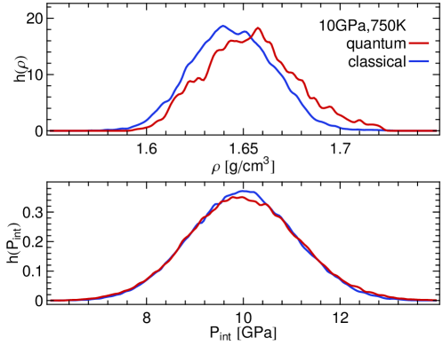
Figure 3: Histogram of the density (upper panel) and of the instantaneous internal pressure estimator in Eq. (5) (lower panel), comparing NPT simulations with classical and quantum nuclei.

5.2 Results and discussion

Figure 3 reports the histograms of density and internal pressure obtained during the simulations. The average density in the classical simulation is $1.644\pm 0.001$ g/cm³, which is qualitatively consistent with the simulation of Ref. [39], which observed an average pressure of 14.5 GPa in the NVT ensemble at a density of $1.72$ g/cm³. The density appears to be slightly higher for simulations with quantum nuclei, $1.654\pm 0.003$ g/cm³, but one should note that the correlation time for $\rho$ tends to be underestimated in relatively short ab initio runs, so the quantum effect is barely significant given that our computed error bars are likely to be optimistic. Note that the estimator for the internal pressure is correctly peaked around the value fixed by the definition of the ensemble.

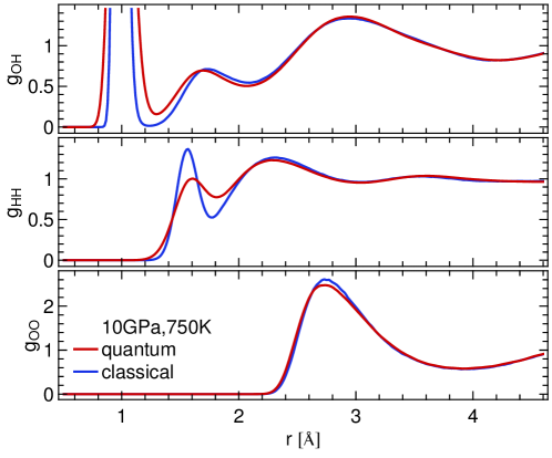
Figure 4: Radial distribution functions from NPT simulations of water at a temperature of 750 K and a pressure of 10 GPa. Simulations with classical and quantum nuclei are compared.

The small role that NQEs play in determining the equilibrium density is not surprising: even at room temperature, the isotope effect on the number density of water is extremely small. However, one should not think that at these high temperatures the quantum nature of light nuclei can be neglected. It is clear from the radial distribution functions reported in Figure 4 that, while nuclear quantum effects do not change the long-range structure, they do have a very sizeable impact on the short-range part of $g(r)$. There is very little effect on the oxygen-oxygen $g_{\text{OO}}(r)$ (the difference is barely significant considering the statistical error bars), but $g_{\text{HH}}(r)$ and $g_{\text{OH}}(r)$ are noticeably over-structured for $r<2\text{ \AA}$ in the classical simulation. Notice in particular how the quantum $g_{\text{OH}}(r)$ departs significantly from zero between the intra-molecular and inter-molecular regions. This is a sign that the combined effect of pressure and NQEs leads to significant delocalization of protons along the hydrogen bonds.

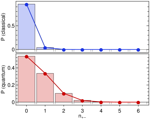
Figure 5: These bar charts depict the probability of finding $n_{+-}$ charged pairs in a snapshot of our simulation box. The upper panel is for a classical simulation, and the lower panel for a quantum simulation. The dots joined with lines represent the values for a binomial distribution fitted to the computed probabilities – each snapshot contains 64 water molecules, so can accommodate a maximum of 32 ion pairs. The best-fit probability of a pair being ionized is found to be $p_{+-}=0.019$ for the quantum simulation and $p_{+-}=0.0014$ for the classical simulation.

To investigate this delocalisation further, we have adopted the simple protocol used in Ref. [39] to identify charged species. Each proton in the simulation is assigned to the closest oxygen atom. One can then distinguish between neutral, positively and negatively charged species based on the number of protons assigned to each oxygen. We will refer to “$+$” species as those oxygen atoms to which three protons have been assigned, and “$-$” species as those with just one. Given the artificial nature of this procedure, we do not intend to imply that these species correspond to water, hydronium and hydroxide. However, they do provide a simple way to characterise how much each frame departs from the conventional picture of a molecular fluid composed of neutral molecules. In all of our simulations, we only detected a single instance of a “doubly ionised” oxygen, so in the discussion that follows we shall assume that the charged O atoms always form in pairs.

Figure 5 shows very clearly just how important NQEs are in determining the fluctuations of protons along hydrogen bonds. Most frames in the classical simulation only contain neutral species – the concentration of $+$ or $-$ is $\approx 0.07$%, even smaller than that observed in Ref. [39], where the density was higher. In the quantum simulation, the concentration is much larger, about $0.97$%, and there is a fairly large probability of having more than one pair of ions in any given frame. Interestingly, in both cases the probability of finding $n_{+-}$ ionised pairs follows closely a binomial distribution, which is a sign that the ionisation events are weakly correlated with each other.

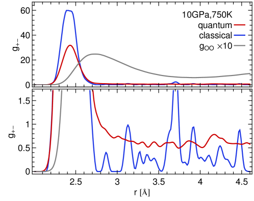
Figure 6: Radial distribution functions for positively and negatively charged defects in NPT simulations of water at 10 GPa and 750 K. Results from quantum and classical simulations are compared, and the lower panel shows the long-range part of $g_{+-}(r)$ on an enlarged scale. Given the low concentration of defects, the radial distribution functions are very noisy, and the normalisation is problematic, so the scale of the ordinate should be considered as arbitrary.

It is interesting to investigate the spatial distribution of these ion pairs: in Figure 6 we show the radial distribution functions $g_{+-}(r)$. The distributions are very noisy, particularly in the classical case, where we have only a handful of snapshots containing more than a single ion pair. In the quantum simulation, we could collect better statistics, because the concentration of ion pairs is larger. In this case, is clear that the radial distribution function is almost flat for $r>3$ Å (see lower panel of Figure 6), which is consistent with the binomial distribution of $n_{+-}$ in Figure 5. Furthermore, the upper panel of Figure 6 clearly shows that, in the vast majority of cases, what is detected as a pair of ions is simply an excursion of a proton along a compressed hydrogen bond. This is consistent with the observation of short-lived charged species in classical simulations of water at considerably higher pressure [49].

As was shown in a recent study of water under ambient conditions [50], nuclear quantum effects dramatically enhance the delocalisation of the proton along the hydrogen bond. This suggests that perturbations that modulate the average O–O distance, such as pressure, might trigger auto-ionisation more easily than in the classical case. In fact, not all of the ion pairs in the present simulations are close together and short-lived: if we define an isolated ion as a positive species that has no negative counterpart within $3$ Å of it, we find a concentration of $6\times 10^{-3}$% of these isolated ions in our classical simulations, and of $0.24$% in our quantum simulations. This is not far from the value of 0.5 % measured in shock-compressed water at 13 GPa [51, 52]. However, our definition of an isolated ion is somewhat arbitrary, and the concentrations we quote will be strongly system-size dependent. Nevertheless, the ratio between these concentrations and the overall fraction of ionised species indicates that quantum effects have an even more dramatic impact on genuine auto-ionisation events than they do on local hydrogen bond fluctuations. This is perhaps not too surprising, given the significant isotope effect on the pH of water under ambient conditions.

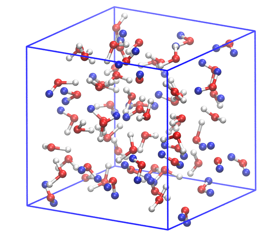
Figure 7: A snapshot from the final stage of our 40 ps quantum simulation of water at 750 K and 10 GPa. Protons that are bound to a different oxygen than the one they were bound to in the initial configuration of the trajectory are highlighted in blue. Note that many exchanges have occurred. In our classical simulation, no exchanges were observed.

The presence of a significant fraction of ionised species increases the mobility of protons, which can hop from molecule to molecule in a Grotthuss-like fashion. Even though PIMD (and particularly the heavily-thermostatted PIGLET method) does not allow us to make quantitative statements about how quantum effects enhance proton mobility, one can clearly see that by the end of our quantum simulation a significant fraction of the protons has been exchanged between water molecules (see Figure 7). On the contrary, in the classical case all the water molecules maintain their chemical identity thoughout our simulation. Using an approximate quantum dynamics technique such as RPMD [31] or CMD [32, 33] to study the dynamics in high pressure water would be an interesting future application of i-PI.

6 Conclusions

In this paper we have introduced i-PI, a Python interface designed to facilitate including nuclear quantum effects in ab initio path integral molecular dynamics simulations. Our program delegates the calculation of the potential, forces and virial tensor to an external code, keeping the electronic structure calculation and the propagation of the nuclear dynamics separate. Communication between the codes is achieved using internet sockets, which exchange just the essential information, thereby minimising the number of modifications that have to be made to the ab initio client. i-PI implements the most recent developments in path integral simulation technology, including correlated-noise methods that accelerate the convergence with respect to the number of beads, and an implementation of NPT PIMD based on stochastic thermostatting.

We have demonstrated the potential of i-PI with an application to the ab initio simulation of high-pressure water. Our simulations with classical nuclei are consistent with previous simulations [39, 49], performed at a similar thermodynamic state point and using similar computational details for the electronic structure. However, our results show that even at a temperature as high as 750 K nuclear quantum effects play an important role in determining the behaviour of water. The concentration of ionised species – as defined by a simple geometric criterion – is increased by more than an order of magnitude when one treats the nuclei as quantum particles. We have characterised the nature of these charged species, observing that in the vast majority of cases they correspond to fluctuations of a proton along a compressed hydrogen bond, giving rise to a transient contact pair rather than to well-separated, solvated charges. Nevertheless, at the high ionic concentrations (more than 1 %) observed in quantum simulations, a smaller fraction of these fluctuations leads to long-range separation of ionised species, and to effective transport and exchange of protons across the hydrogen-bond network, which is observed in classical simulations only at a much higher pressure [39, 49].

These results and those of many other recent studies are leading to an increasing body of evidence that it is desirable (and in some cases even essential) to include nuclear quantum effects in molecular dynamics simulations if one wants to obtain a realistic description of systems containing hydrogen atoms. The inclusion of quantum effects certainly entails a computational overhead, but recent methodological developments that combine path integrals with correlated-noise, generalized Langevin dynamics have reduced this overhead considerably. We envisage that the introduction of i-PI will make these new techniques more readily accessible, and thereby encourage the more routine inclusion of NQEs in ab initio molecular dynamics simulations. The modular nature of i-PI should also ensure that further methodological developments will be easy to incorporate, so that communities that use a diverse variety of electronic structure programs can be kept up-to-date with the field.

References

- [1] C. C. Fischer, K. J. Tibbetts, D. Morgan, G. Ceder, Predicting crystal structure by merging data mining with quantum mechanics., Nature materials 5 (8) (2006) 641–6.
- [2] R. Car, M. Parrinello, Unified Approach for Molecular Dynamics and Density-Functional Theory, Phys. Rev. Lett. 55 (22) (1985) 2471–2474.
- [3] K. Burke, Perspective on density functional theory., J. Chem. Phys. 136 (15) (2012) 150901.
- [4] D. Chandler, P. G. Wolynes, Exploiting the isomorphism between quantum theory and classical statistical mechanics of polyatomic fluids, J. Chem. Phys. 74 (7) (1981) 4078–4095.
- [5] M. Parrinello, A. Rahman, Study of an F center in molten KCl, J. Chem. Phys. 80 (1984) 860.
- [6] D. M. Ceperley, Path integrals in the theory of condensed helium, Rev. Mod. Phys. 67 (2) (1995) 279–355.
- [7] R. P. Feynman, A. R. Hibbs, Quantum Mechanics and Path Integrals, McGraw-Hill, New York, 1964.
- [8] M. E. Tuckerman, D. Marx, M. L. Klein, M. Parrinello, Efficient and general algorithms for path integral Car{–}Parrinello molecular dynamics, J. Chem. Phys. 104 (14) (1996) 5579–5588.
- [9] D. Marx, M. Parrinello, Ab initio path integral molecular dynamics: Basic ideas, J. Chem. Phys. 104 (11) (1996) 4077–4082.
- [10] D. Marx, M. E. Tuckerman, J. Hutter, M. Parrinello, The nature of the hydrated excess proton in water, Nature 397 (6720) (1999) 601–604.
- [11] R. L. Hayes, S. J. Paddison, M. E. Tuckerman, Proton transport in triflic acid hydrates studied via path integral car-parrinello molecular dynamics., J. Phys. Chem.. B 113 (52) (2009) 16574–89.
- [12] J. Chen, X.-Z. Li, Q. Zhang, A. Michaelides, E. Wang, Nature of proton transport in a water-filled carbon nanotube and in liquid water., PCCP (2013) 6344–6349.
- [13] S. Buyukdagli, A. V. Savin, B. Hu, Computation of the temperature dependence of the heat capacity of complex molecular systems using random color noise, Phys. Rev. E 78 (6) (2008) 66702.
- [14] M. Ceriotti, G. Bussi, M. Parrinello, Nuclear quantum effects in solids using a colored-noise thermostat, Phys. Rev. Lett. 103 (3) (2009) 30603.
- [15] H. Dammak, Y. Chalopin, M. Laroche, M. Hayoun, J.-J. Greffet, Quantum Thermal Bath for Molecular Dynamics Simulation, Phys. Rev. Lett. 103 (19) (2009) 190601.
- [16] M. Ceriotti, D. E. Manolopoulos, M. Parrinello, Accelerating the convergence of path integral dynamics with a generalized Langevin equation., J. Chem. Phys. 134 (8) (2011) 84104.
- [17] M. Ceriotti, D. E. Manolopoulos, Efficient First-Principles Calculation of the Quantum Kinetic Energy and Momentum Distribution of Nuclei, Phys. Rev. Lett. 109 (10) (2012) 100604.
- [18] M. Ceriotti, M. Parrinello, T. E. Markland, D. E. Manolopoulos, Efficient stochastic thermostatting of path integral molecular dynamics., J. Chem. Phys. 133 (12) (2010) 124104.
- [19] M. Tuckerman, B. J. Berne, G. J. Martyna, Reversible multiple time scale molecular dynamics, J. Chem. Phys. 97 (3) (1992) 1990.
- [20] T. E. Markland, D. E. Manolopoulos, An efficient ring polymer contraction scheme for imaginary time path integral simulations., J. Chem. Phys. 129 (2) (2008) 024105.
- [21] T. E. Markland, D. E. Manolopoulos, A refined ring polymer contraction scheme for systems with electrostatic interactions, Chem. Phys. Lett. 464 (4-6) (2008) 256.
- [22] G. Bussi, D. Donadio, M. Parrinello, Canonical sampling through velocity rescaling, J. Chem. Phys. 126 (1) (2007) 14101.
- [23] M. Ceriotti, G. Bussi, M. Parrinello, Langevin Equation with Colored Noise for Constant-Temperature Molecular Dynamics Simulations, Phys. Rev. Lett. 102 (2) (2009) 020601.
- [24] M. Ceriotti, G. Bussi, M. Parrinello, Colored-Noise Thermostats à la Carte, J. Chem. Theory Comput. 6 (4) (2010) 1170–1180.
- [25] M. Ceriotti, M. Parrinello, The -thermostat: selective normal-modes excitation by colored-noise Langevin dynamics, Procedia Computer Science 1 (1) (2010) 1607–1614.
- [26] GLE4MD, http://gle4md.berlios.de.
- [27] T. M. Yamamoto, Path-integral virial estimator based on the scaling of fluctuation coordinates: Application to quantum clusters with fourth-order propagators, J. Chem. Phys. 123 (10) (2005) 104101.
- [28] M. Ceriotti, T. E. Markland, Efficient methods and practical guidelines for simulating isotope effects., J. Chem. Phys. 138 (1) (2013) 014112.
- [29] L. Lin, J. A. Morrone, R. Car, M. Parrinello, Displaced Path Integral Formulation for the Momentum Distribution of Quantum Particles, Phys. Rev. Lett. 105 (11) (2010) 110602.
- [30] I. R. Craig, D. E. Manolopoulos, Quantum statistics and classical mechanics: Real time correlation functions from ring polymer molecular dynamics, J. Chem. Phys. 121 (2004) 3368.
- [31] S. Habershon, D. E. Manolopoulos, T. E. Markland, T. F. Miller, Ring-polymer molecular dynamics: quantum effects in chemical dynamics from classical trajectories in an extended phase space., Annual review of physical chemistry 64 (2013) 387–413.
- [32] J. Cao, G. A. Voth, A new perspective on quantum time correlation functions, J. Chem. Phys. 99 (12) (1993) 10070–10073.
- [33] J. Cao, G. A. Voth, The formulation of quantum statistical mechanics based on the Feynman path centroid density. IV. Algorithms for centroid molecular dynamics, J. Chem. Phys. 101 (7) (1994) 6168–6183.
- [34] G. Bussi, T. Zykova-Timan, M. Parrinello, Isothermal-isobaric molecular dynamics using stochastic velocity rescaling, J. Chem. Phys. 130 (7) (2009) 74101.
- [35] G. J. Martyna, A. Hughes, M. E. Tuckerman, Molecular dynamics algorithms for path integrals at constant pressure, J. Chem. Phys. 110 (7) (1999) 3275.
- [36] H. C. Andersen, Molecular dynamics simulations at constant pressure and/or temperature, J. Chem. Phys. 72 (4) (1980) 2384–2393.
- [37] M. Parrinello, Polymorphic transitions in single crystals: A new molecular dynamics method, J. Appl. Phys. 52 (12) (1981) 7182.
- [38] G. Bussi, M. Parrinello, Accurate sampling using Langevin dynamics, Phys. Rev. E 75 (5) (2007) 56707.
- [39] E. Schwegler, G. Galli, F. Gygi, R. Hood, Dissociation of Water under Pressure, Phys. Rev. Lett. 87 (26) (2001) 265501.
- [40] S. Habershon, T. E. Markland, D. E. Manolopoulos, Competing quantum effects in the dynamics of a flexible water model., J. Chem. Phys. 131 (2) (2009) 24501.
- [41] {CP2K}, http://cp2k.berlios.de.
- [42] J. Schmidt, J. VandeVondele, I.-F. W. Kuo, D. Sebastiani, J. I. Siepmann, J. Hutter, C. J. Mundy, Isobaric-isothermal molecular dynamics simulations utilizing density functional theory: an assessment of the structure and density of water at near-ambient conditions., J. Phys. Chem.. B 113 (35) (2009) 11959–64.
- [43] A. D. Becke, Density-functional exchange-energy approximation with correct asymptotic behavior, Phys. Rev. A 38 (6) (1988) 3098.
- [44] C. Lee, W. Yang, R. G. Parr, Development of the Colle-Salvetti correlation-energy formula into a functional of the electron density, Phys. Rev. B 37 (2) (1988) 785.
- [45] S. Goedecker, M. Teter, J. Hutter, Separable dual-space Gaussian pseudopotentials, Phys. Rev. B 54 (3) (1996) 1703–1710.
- [46] S. Grimme, J. Antony, S. Ehrlich, H. Krieg, A consistent and accurate ab initio parametrization of density functional dispersion correction (DFT-D) for the 94 elements H-Pu., J. Chem. Phys. 132 (15) (2010) 154104.
- [47] M. Guidon, J. Hutter, J. VandeVondele, Robust Periodic Hartree−Fock Exchange for Large-Scale Simulations Using Gaussian Basis Sets, J. Chem. Theory Comput. 5 (11) (2009) 3010–3021.
- [48] M. Guidon, J. Hutter, J. VandeVondele, Auxiliary Density Matrix Methods for Hartree−Fock Exchange Calculations, J. Chem. Theory Comput. 6 (8) (2010) 2348–2364.
- [49] A. Goncharov, N. Goldman, L. Fried, J. Crowhurst, I.-F. Kuo, C. Mundy, J. Zaug, Dynamic Ionization of Water under Extreme Conditions, Phys. Rev. Lett. 94 (12) (2005) 125508.
- [50] M. Ceriotti, J. Cuny, M. Parrinello, D. E. Manolopoulos, Nuclear quantum effects and hydrogen bond fluctuations in water, Proc. Nat. Acad. Sci. 110 (39) (2013) 15591–15596.
- [51] S. D. Hamann, Electrolyte solutions at high pressure, in: Modern aspects of electrochemistry, Springer, 1974, pp. 47–158.
- [52] A. C. Mitchell, W. J. Nellis, Equation of state and electrical conductivity of water and ammonia shocked to the 100 GPa (1 Mbar) pressure range, J. Chem. Phys. 76 (12) (1982) 6273.