ICM cooling, AGN feedback, and BCG properties of galaxy groups

Abstract

Aims. We aim to investigate cool-core and non-cool-core properties of galaxy groups through X-ray data and compare them to the AGN radio output to understand the network of intracluster medium (ICM) cooling and feedback by supermassive black holes. We also aim to investigate the brightest cluster galaxies (BCGs) to see how they are affected by cooling and heating processes, and compare the properties of groups to those of clusters.

Methods. Using Chandra data for a sample of 26 galaxy groups, we constrained the central cooling times (CCTs) of the ICM and classified the groups as strong cool-core (SCC), weak cool-core (WCC), and non-cool-core (NCC) based on their CCTs. The total radio luminosity of the BCG was obtained using radio catalogue data and/or literature, which in turn was compared to the cooling time of the ICM to understand the link between gas cooling and radio output. We determined K-band luminosities of the BCG with 2MASS data, and used a scaling relation to constrain the masses of the supermassive black holes, which were then compared to the radio output. We also tested for correlations between the BCG luminosity and the overall X-ray luminosity and mass of the group. The results obtained for the group sample were also compared to previous results for clusters.

Results. The observed cool-core/non-cool-core fractions for groups are comparable to those of clusters. However, notable differences are seen: 1) for clusters, all SCCs have a central temperature drop, but for groups this is not the case as some have centrally rising temperature profiles despite very short cooling times; 2) while for the cluster sample, all SCC clusters have a central radio source as opposed to only 45% of the NCCs, for the group sample, all NCC groups have a central radio source as opposed to 77% of the SCC groups; 3) for clusters, there are indications of an anticorrelation trend between radio luminosity and CCT. However, for groups this trend is absent; 4) the Indication of a trend of radio luminosity with black hole mass observed in SCC clusters is absent for groups; and 5) similarly, the strong correlation observed between the BCG luminosity and the cluster X-ray luminosity/cluster mass weakens significantly for groups.

Conclusions. We conclude that there are important differences between clusters and groups within the ICM cooling/AGN feedback paradigm and speculate that more gas is fueling star formation in groups, than in clusters where much of the gas is thought to feed the central AGN.

1 Introduction

The discovery that the cooling time of the intracluster medium (ICM) in the centres of many clusters, the so-called cool-core clusters, is much shorter than the Hubble time (e.g. Lea et al. 1973; Cowie & Binney 1977; Fabian & Nulsen 1977) led to the development of the cooling flow model. In this model, as the gas cools hydrostatically, it is compressed by the hot, overlying gas, generating a cooling flow (see Fabian 1994 for a review). After early indications from the advanced satellite for cosmology and astrophysics, i.e. ASCA (e.g. Makishima et al. 2001), the high-spectral resolution data from the reflection grating spectrometer (RGS) instrument on XMM-Newton have shown that the actual mass deposition rates fall short of the predictions by an order of magnitude. These data showed that not enough cool gas was present in the cool-core clusters (e.g. Peterson et al. 2001; Xu et al. 2002; Tamura et al. 2001; Kaastra et al. 2001; I. Sakelliou et al. 2002; Peterson et al. 2003; Peterson & Fabian 2006; Sanders et al. 2008). Optical and UV data revealed the same level of discrepancy between the expected and observed star formation rates (e.g. McNamara & O’Connell 1989; Allen 1995; Edge & Frayer 2003; Rafferty et al. 2006, 2008).

Several different criteria have been used in the literature to distinguish between cool-core (CC) and non-cool-core (NCC) clusters, making it difficult to compare results. Some of the parameters used are central entropy (e.g. Voit et al. 2008, Cavagnolo et al. 2009, Rossetti et al. 2011), central temperature drop (e.g. Sanderson et al. 2006, Burns et al. 2008), classical mass deposition rate (e.g. Chen et al. 2007), and central cooling time (e.g. Hudson et al. 2010). Hudson et al. (2010) analysed 16 parameters using the HIFLUGCS sample (Reiprich & Böhringer, 2002) and concluded that for low-$z$ clusters, the central cooling time (CCT) was the best parameter to use to distinguish between CC and NCC clusters.

The classical cooling flow model does not consider any heating mechanism in addition to radiative cooling of the intracluster gas. In recent years, several models incorporating heating mechanisms have been explored, such as heating by supernovae, thermal conduction, and active galactic nuclei (AGN). Self-regulated AGN feedback has gained favor in recent years (e.g. Churazov et al. 2002; Roychowdhury et al. 2004; Voit & Donahue 2005). Excellent correlations between X-ray deficient regions in the ICM, i.e. cavities and radio lobes, have given credence to this hypothesis (e.g. Böhringer et al. 1993; McNamara et al. 2000; Blanton et al. 2001; Clarke et al. 2004; Bîrzan et al. 2004, 2008). Mittal et al. (2009) showed that the likelihood of a cluster hosting a central radio source (CRS) increases as the CCT decreases. The exact details of the heating mechanism through AGN are still unclear. Possibilities include heat transfer through weak shocks or sound waves (e.g. Fabian et al. 2003; Jones et al. 2002; Mathews et al. 2006), cosmic ray interaction with the ICM (Guo & Oh, 2008), and the $PdV$ work done by the expanding radio jets on the ICM (e.g. Ruszkowski et al. 2004, see also McNamara & Nulsen 2007 for a review).

Trying to understand the correlation between gas cooling in the intracluster medium (ICM) and feedback processes on the galaxy group scale is fundamental in our understanding of the exact differences between clusters and groups. Galaxy groups, being systems not as massive as clusters, have long been considered scaled-down versions of clusters. The definition of a group and cluster is extremely loose and a rule of thumb definition is to designate systems comprising less than 50 galaxies as a group and above 50 as a cluster, but in recent years there has been some suggestion that groups cannot be simply treated as scaled-down versions of clusters. For example, in clusters the ICM usually dominates the baryonic budget, whereas in groups the combined mass of the member galaxies may exceed the baryonic mass in the ICM (e.g. Giodini et al. 2009). Furthermore, the main cooling mechanism in groups (line emission) differs from that in clusters (thermal bremsstrahlung). In principle, feedback from an AGN would have a greater impact on the group because of the smaller gravitational potential.

Randall et al. (2011) show that shock heating perpetuated by an AGN explosion alone is enough to balance radiative losses in the galaxy group NGC 5813. Groups such as HCG 62 (Gitti et al., 2010) show radio lobes corresponding to X-ray cavities, which could indicate that the ICM cooling/AGN feedback on the group regime is similar to that in galaxy clusters. However, as pointed out by Sun (2009), this is not so trivial and the situation is complicated even more by the presence of the so-called coronae class of kpc-sized objects representing emission from individual galaxies, likely harbouring a supermassive black hole (SMBH). Gaspari et al. (2011) argue through simulations that AGN feedback on the group regime is persistent and delicate unlike in clusters. It is worth stating here that the multitude of cool-core definitions used to define clusters and comparisons between the cool-core properties has not been thoroughly tested on the group regime with an objectively selected group sample. Thus, it becomes highly imperative to see how groups are different to clusters within the cool-core/feedback paradigm and to what extent; motivated by the basic fact that groups of galaxies are more numerous than clusters (as evident from the shape of the cluster mass function). Most of the $10^{5}$ clusters to be detected by the upcoming eROSITA X-ray mission will be groups of galaxies or low-mass clusters (Pillepich et al., 2012). The aim of upcoming cluster missions, eROSITA in particular, is to perform precision cosmology using clusters as cosmological probes. The processes of ICM cooling and AGN feedback could easily cause scaling relations to diverge from their norm (e.g. Mittal et al. 2011), which in turn could undermine their utility in cosmological applications.

The brightest cluster galaxies (BCGs) have a special role in the aforementioned paradigm. These are highly luminous galaxies, usually of giant elliptical and cD type, and are generally located quite close to the X-ray peak ($<50h^{-1}$kpc in 88% of the cases, Hudson et al. 2010). Elliptical galaxy properties, like the optical bulge luminosity and velocity dispersion, have well defined scaling relations, allowing one to indirectly estimate the mass of the SMBH (e.g. Kormendy & Richstone 1995, Ferrarese & Merritt 2000), which may be compared to the AGN activity (e.g. Fujita & Reiprich 2004; Mittal et al. 2009). Brightest cluster galaxies also help in studying the role of cooling gas in fueling star formation where the cooling gas at least partially forms new stars (e.g. Hicks et al. 2010). Mittal et al. (2009) also allude to the possibility of different growth histories for SCC BCGs than for non-SCC BCGs. An investigation of BCGs on the group regime and comparison to cluster BCGs, factoring in the CC/NCC paradigm has not yet been carried out.

In this paper, we attempt to address several questions related to gas cooling properties, AGN feedback and BCG properties on the galaxy group scale. It is organised as follows: Section 2 deals with the sample selection and data analysis. Section 3 contains the results. A discussion of our results is carried out in Sect. 4. A short summary is presented in Sect. 5. Throughout this work, we assume a $\Lambda$CDM cosmology with $\Omega_{\mathrm{m}}=0.3$, $\Omega_{\Lambda}=0.7$, and $h=0.71$, where $H_{0}=100h$ km/s/Mpc. Correlations between different physical parameters were quantified with the help of linear regression analysis using the BCES bisector code by Akritas & Bershady (1996), and the degree of the correlations was estimated using the Spearman rank correlation coefficient. All errors are quoted at the $1\sigma$ level unless stated otherwise.

2 Sample selection and data analysis

2.1 Sample selection

The group sample used in this work is the same as used by Eckmiller et al. (2011). The main aim of that study was to test scaling relations on the galaxy group scale. The groups were selected from the following three catalogues:

• NORAS: Northern ROSAT All Sky galaxy cluster survey by Böhringer et al. (2000).

• REFLEX: ROSAT-ESO Flux Limited X-ray galaxy cluster survey by Böhringer et al. (2004).

• HIFLUGCS: Highest X-ray Flux Galaxy Cluster Sample by Reiprich & Böhringer (2002).

An upper-cut on the luminosity of $2.55\cdot 10^{43}h^{-2}_{70}$ erg s^-1 in the ROSAT band was applied to select only groups, and a lower redshift cut of $z>$ 0.01 was applied to exclude objects too close to be observed out to a large enough projected radius in the sky. This yielded a statistically complete sample of 112 groups. However, not all of them have high-quality X-ray data, and so only those groups with Chandra observations were selected, giving a sample of 27 galaxy groups. One group, namely IC 4296 was excluded as the observations were not suitable for ICM analysis, which resulted in a final sample of 26 groups. More details about the sample are provided in Eckmiller et al. (2011).

2.2 Data reduction

For the data reduction we used the CIAO software package in version 4.4 with CALDB 4.5.0. Following the suggestions on the Chandra Science Threads, we reprocessed the raw data (removing afterglows, creating the bad-pixel table, applying the latest calibration) by using the chandra_repro task. Soft-proton flares were filtered by cleaning the lightcurve with the lc_clean algorithm (following the steps in the Markevitch cookbook ). All lightcurves were also visually inspected afterwards for any residual flaring. Point sources were detected by the wavdetect wavelet algorithm (the images were visually inspected to ensure that the detected point sources were reasonable) and excluded from the spectral and surface-brightness analysis. The regions used for the spectral analysis were selected by a count threshold of at least 2500 source counts and fit by an absorbed (wabs) APEC model, centred on the emission peak (EP), determined using the tool fimgstat. Table 1 gives the co-ordinates of the EP in RA/DEC. The Anders & Grevesse (1989) abundance table was used throughout.

2.2.1 Background subtraction

For the background subtraction we followed the steps illustrated by e.g. Zhang et al. (2009) and Sun et al. (2009) with some minor modifications.

The particle background, i.e. the highly energetic particles that interact with the detector, was estimated from stowed events files distributed within the CALDB. The astrophysical X-ray background was estimated from a simultaneous spectral fit to the Chandra data and data from the ROSAT all-sky survey (RASS) provided by Snowden’s webtool, using the X-ray spectral fitting package Xspec. The components used to fit the background were an absorbed power law with a spectral index of 1.41 (unresolved AGN), an absorbed APEC model (Galactic halo emission) and an unabsorbed APEC model (Local Hot Bubble emission; see Snowden et al. 1998). The RASS data were taken from an annulus far away from the group centre, where no group emission would be present. On average we found temperatures of $0.25\,{\rm keV}$ for the Galactic halo component and $0.11\,{\rm keV}$ for the Local Hot Bubble emission.

The background for the surface-brightness analysis was estimated from the fluxes of the background models plus that from the particle background estimated from the stowed events files (weighted for each region according to the ACIS chips used, and exposure corrected with the exposure maps created for the galaxy groups in an energy range of 0.5-2.0 keV). These values were then subtracted from the surface brightness profiles (SBPs), which were also obtained from an exposure corrected image in an energy range of 0.5-2.0 keV.

2.3 Surface brightness profiles and density profiles

Centered on the EP, the SBP was fitted with either a single or a double $\beta$ model given by

$$\Sigma=\Sigma_{0}\left[1+\left(\frac{x}{x_{\mathrm{c}}}\right)^{2}\right]^{-3\beta+1/2}\\$$ (1)

or

$$\Sigma=\mathrm{\Sigma}_{01}\left[1+\left(\frac{x}{x_{\mathrm{{c_{1}}}}}\right)^{2}\right]^{-3\mathrm{\beta}_{1}+1/2}+\mathrm{\Sigma}_{02}\left[1+\left(\frac{x}{x_{\mathrm{{c_{2}}}}}\right)^{2}\right]^{-3\mathrm{\beta}_{2}+1/2}\leavevmode\nobreak\ ,$$ (2)

respectively (Cavaliere & Fusco-Femiano, 1976). Here, $x_{\mathrm{c_{i}}}$ is the core radius. The density profile for both the models is given by:

$$n = n_{0}\left[1+\left(\frac{r}{r_{\mathrm{c}}}\right)^{2}\right]^{\frac{-3\beta}{2}}$$ (3)

$$n = \left(n_{01}^{2}\left[1+\left(\frac{r}{r_{\mathrm{{c_{1}}}}}\right)^{2}\right]^{-3\beta_{1}}+n_{02}^{2}\left[1+\left(\frac{r}{r_{\mathrm{{c_{2}}}}}\right)^{2}\right]^{-3\beta_{2}}\right)^{1/2}$$ (4)

where $n_{0}=\sqrt{n^{2}_{01}+n^{2}_{02}}$ is the central electron density and $r_{\mathrm{c}}$ is the physical core radius. The central electron density $n_{0}$ can be directly determined using the formulae (Hudson et al., 2010):

$$n_{0}=\left(\frac{10^{14}4\pi D_{\mathrm{A}}D_{\mathrm{L}}\zeta N}{\mathrm{EI}}\right)^{\frac{1}{2}}$$ (5)

$$n_{0}=\left[\frac{10^{14}4\pi(\Sigma_{12}\mathrm{LI_{2}}+\mathrm{LI_{1}})D_{\mathrm{A}}D_{\mathrm{L}}\zeta N}{\Sigma_{12}\mathrm{LI}_{2}\mathrm{EI}_{1}+\mathrm{LI}_{1}\mathrm{EI}_{2}}\right]^{\frac{1}{2}}.$$ (6)

Here, $N$ is the normalisation of the APEC model in the innermost annulus; $\zeta$ is the ratio of electrons to protons ($\sim 1.2$); $\mathrm{\Sigma}_{12}$ is the ratio of the central surface brightness of model-1 to model-2; $D_{\mathrm{A}}$ and $D_{\mathrm{L}}$ are the angular diameter distance and the luminosity distance, respectively; $\mathrm{EI}_{i}$ is the emission integral for model-i and is defined as

$$\mathrm{EI}=2\pi\int_{-\infty}^{\infty}\!\int_{0}^{R}x\left(1+\frac{x^{2}+l^{2}}{x^{2}_{c}}\right)^{-3\beta}\mathrm{d}x\mathrm{d}l\leavevmode\nobreak\ ,$$ (7)

where $R$ is the radius of the innermost annulus and $\mathrm{LI}_{i}$ is the line emission measure for model-$i$ and is defined as

$$\mathrm{LI}_{i}=\int_{-\infty}^{\infty}\left(1+\frac{l^{2}}{x^{2}_{c_{i}}}\right)^{-3\beta_{i}}\mathrm{d}l\leavevmode\nobreak\ .$$ (8)

More details can be found in Hudson et al. (2010).

2.4 Cooling times and central entropies

The major focus of our work is connected to the CCT. This is calculated using the formula:

$$t_{\mathrm{cool}}=\frac{3}{2}\frac{(n_{\mathrm{e}}+n_{\mathrm{i}})kT}{n_{\mathrm{e}}n_{\mathrm{H}}\Lambda(T,Z)}$$

$$\mathrm{CCT}=t_{\mathrm{{cool}}}(0)=\frac{3}{2}\zeta\frac{(n_{\mathrm{{e0}}}+n_{\mathrm{{i0}}})kT_{0}}{{n}^{2}_{\mathrm{{e0}}}\Lambda(T_{0},Z_{0})}$$ (9)

where ${n}_{i0}$ and ${n}_{e0}$ are the central ion and electron densities, respectively, and $T_{0}$ is the central temperature. We note that a bias due to different physical resolutions could be introduced arising because of different distances of the galaxy groups. Hence, we took any parameter (except the central temperature) calculated at $r=0$ to be the value at $r=0.004r_{500}$. The central temperature $T_{0}$ is simply the temperature in the innermost bin in the temperature profile. As in Hudson et al. (2010), $r_{500}$ was calculated from a scaling relation by Evrard et al. (1996) and is given by

$$r_{500}=2\times\left(\frac{kT_{\mathrm{vir}}}{10\leavevmode\nobreak\ \mathrm{keV}}\right)^{\frac{1}{2}}\leavevmode\nobreak\ ,$$ (10)

where the virial temperature was taken from Eckmiller et al. (2011) to calculate the $r_{500}$.

To ensure that the determination of the CCT is not strongly biased because of selection of annuli on the basis of a counts threshold, we performed tests for a few cases where the temperature and surface brightness annuli were increased by a factor of $\sim 3-4$. We did not identify any strong bias that could drastically affect our results.

The central entropy $K_{0}$, another important CC parameter, is calculated as:

$$K_{0}=kT_{0}n^{-2/3}_{\mathrm{e0}}\leavevmode\nobreak\ .$$ (11)

2.5 Radio data and analysis

All the radio data required for this work was either compiled from existing radio catalogs or literature (references in Table 6). We obtained data at several frequencies between 10 MHz and 15 GHz. The major catalogs used for this study were the NVSS (1.4 GHz), SUMSS (843 MHz), and VLSS (74 MHz) catalogs.

Since this study involves radio sources associated with BCGs at the center of the dark matter halo, it is imperative to set a criterion for whether or not a group has a central radio source. Based on the work of Edwards et al. (2007), Mittal et al. (2009) suggest that a central radio source must be located within 50 $h^{-1}_{71}$ kpc of the X-ray peak in order for it to be categorised as a central radio source (CRS). We adopted the same criterion in this work and discovered that most CRSs lie close to the EP (within a few kpc). Appendix C shows the location of the CRS with radio contours overlaid on the optical images with the X-ray emission peak also marked for most of the groups. For CRSs with extended emission, we considered the radio emission from the lobes as well, since our goal is to obtain a correlation between the CCT and the total radio emission from the central AGN.

Radio emission by AGN is characterised by synchrotron radiation expressed as a power law relation given by $S_{\nu}\varpropto\nu^{-\alpha}$, where $S_{\nu}$ is the flux density at frequency $\nu$ and $\alpha$ is the spectral index. Much of the synchrotron emission comes from the lower frequencies ($<1.4\leavevmode\nobreak\$GHz), making it highly important to obtain data on these frequency scales. Moreover, a full radio spectral energy distribution is advantageous since that allows spectral breaks and turn-overs to be discovered. Spectral breaks indicate spectral aging and turn-overs indicate self-absorption. Self-absorption is characterized by a negative spectral index, particularly at lower frequencies. The integrated radio luminosity between a pair of frequencies $\mathrm{\nu}_{i}$ and $\mathrm{\nu}_{i+1}$ is given by

$$L_{i+1}=4\pi D^{2}_{L}\frac{S_{0}\mathrm{\nu}_{0}^{\mathrm{\alpha}_{i+1,i}}}{1-\mathrm{\alpha}_{i+1,i}}\left(\nu^{1-\alpha_{i+1,i}}_{i+1}-\nu^{1-\alpha_{i+1,i}}_{i}\right)\leavevmode\nobreak\ ,$$ (12)

where $S_{0}$ is the flux density at either frequency $\mathrm{\nu}_{i+1,i}$ or $\mathrm{\nu}_{i}$, $\mathrm{\alpha}_{i+1,i}$ is the spectral index between the two frequencies, and $D_{\mathrm{L}}$ is the luminosity distance. To calculate the total radio luminosity between 10 MHz and 15 GHz, the spectral index at the lowest observed frequency was extrapolated to 10 MHz, and the spectral index at the highest observed frequency was extrapolated to 15 GHz. The integrated radio luminosity was then calculated as $L_{\mathrm{tot}}=\Sigma L_{\mathrm{i+1}}$. In the case of unavailability of multi-frequency data, we assumed a spectral index of 1 throughout the energy range (e.g. Mittal et al. 2009). This had to be done for 11 CRSs in the sample. Table 6 summarises the radio data.

2.6 BCG data and analysis

For the BCG analysis, we followed the same methodology as explained in Mittal et al. (2009) and describe it here briefly.

The BCG near-infrared (NIR) $K$-band magnitudes ($km_{\mathrm{ext}}$) are obtained from the 2MASS Extended Source Catalog (Jarrett et al., 2000; Skrutskie et al., 2006), i.e. the XSC. Redshifts were obtained from the NASA/IPAC Extragalactic Database (NED). The magnitudes were corrected for Galactic extinction using dust maps by Schlegel et al. (1998). As these are extremely low redshift galaxies, no $k$-correction was applied. The magnitudes were then converted to luminosities under the Vega system, assuming an absolute $K$-band solar magnitude equal to 3.32 mag (Colina & Bohlin, 1997).

Studies like Marconi & Hunt (2003) and Batcheldor et al. (2007) have established well-defined scaling relations between galaxies’ NIR bulge luminosity and the SMBH mass, consistent with results obtained from velocity dispersions (e.g. Tremaine et al. 2002).

We use the scaling relation from Marconi & Hunt (2003) to obtain the SMBH mass,

$$\mathrm{log_{10}}\left(\frac{M_{\mathrm{BH}}}{M_{\odot}}\right)=a+b\left[\mathrm{log}_{10}\left(\frac{L_{\mathrm{BCG}}}{L_{\odot}}\right)-10.9\right]\leavevmode\nobreak\ ,$$ (13)

where $a=8.21\pm 0.07$ and $b=1.13\pm 0.12$. The derived SMBH mass was compared to the integrated radio luminosity. The BCG luminosities were compared to the global cluster properties, like the total X-ray luminosity $L_{\mathrm{X}}$ and mass $M_{500}$.

3 Results

3.1 Cool-core and non-cool-core fraction

Hudson et al. (2010) analysed 16 parameters using Kaye’s Mixture Mode (KMM) algorithm as described by Ashman et al. (1994), where the CCT showed a strong trimodal distribution. Thus, the authors divided the clusters into three categories: strong cool-core (SCC) clusters with CCTs below 1 Gyr, weak cool-core (WCC) clusters with CCTs between 1 Gyr and 7.7 Gyr, and non-cool-core (NCC) clusters with CCT above 7.7 Gyr. Using the same classification system, we present our sample classified as SCC, WCC, and NCC groups in Table 1. This table also shows the central electron density and the central entropy (Sect. 3.3). The observed SCC fraction is 50%, the WCC fraction is 27%, and the NCC fraction is 23% (Fig. 1). A histogram showing the distribution of the CCTs is shown in Fig. 2.

Table 1: The columns are (1) group name, (2) co-ordinates (J2000) of the EP, (3) central electron density, (4) central temperature, (5) central cooling time, (6) central entropy, (7) cool-core type, and (8) presence or absence of a central radio source.

Group name	EP (RA/DEC)	$n_{0}$ ($10^{-2}\leavevmode\nobreak\ \mathrm{cm}^{-3}$)	$T_{0}$ keV	CCT (in Gyr)	$K_{0}$ ($\mathrm{keV}\mathrm{cm}^{2}$)	CC type	CRS?
A0160	$01:12:59.67\leavevmode\nobreak\ +15:29:29.11$	$0.380^{+0.068}_{-0.068}$	$2.38^{+0.218}_{-0.218}$	$8.04^{+1.26}_{-1.83}$	$97.7^{+10.1}_{-13.7}$	NCC	YES
A1177	$11:09:44.38\leavevmode\nobreak\ +21:45:32.81$	$0.600^{+0.130}_{-0.130}$	$1.63^{+0.08}_{-0.08}$	$3.77^{+0.67}_{-1.04}$	$49.4^{+6.05}_{-8.73}$	WCC	NO
ESO55	$04:54:52.31\leavevmode\nobreak\ -18:06:54.29$	$0.760^{+0.14}_{-0.14}$	$1.88^{0.13}_{-0.13}$	$2.70^{+0.40}_{-0.57}$	$48.6^{+5.18}_{-7.07}$	WCC	NO
HCG62	$12:53:06.00\leavevmode\nobreak\ -09:12:11.57$	$3.80^{+1.23}_{-1.23}$	$0.813^{+0.008}_{-0.008}$	$0.214^{+0.0523}_{-0.1023}$	$7.19^{+1.23}_{-2.14}$	SCC	YES
HCG97	$23:47:23.03\leavevmode\nobreak\ -02:18:00.49$	$1.44^{+0.19}_{-0.19}$	$0.992^{+0.015}_{-0.015}$	$0.977^{+0.114}_{-0.149}$	$16.8^{+1.33}_{-1.66}$	SCC	NO
IC1262	$17:33:03.07\leavevmode\nobreak\ +43:45:34.88$	$4.12^{+0.13}_{-0.13}$	$1.63^{+0.03}_{-0.03}$	$0.504^{+0.015}_{-0.016}$	$13.7^{+0.280}_{-0.295}$	SCC	YES
IC1633	$01:09:56.07\leavevmode\nobreak\ -45:55:52.28$	$0.38^{+0.0883}_{-0.0883}$	$2.82^{+0.13}_{-0.13}$	$8.20^{+1.54}_{-2.48}$	$115^{+15.1}_{-22.3}$	NCC	YES
MKW4	$12:04:27.14\leavevmode\nobreak\ +01:53:45.18$	$3.91^{+0.34}_{-0.34}$	$1.57^{+0.02}_{-0.02}$	$0.258^{+0.0207}_{-0.0246}$	$13.6^{+0.737}_{-0.852}$	SCC	YES
MKW8	$14:40:42.99\leavevmode\nobreak\ +03:27:56.98$	$0.34^{+0.0453}_{-0.0453}$	$3.69^{+0.18}_{-0.18}$	$10.1^{+1.19}_{-1.56}$	$163^{+13.0}_{-16.3}$	NCC	YES
NGC326	$00:58:22.82\leavevmode\nobreak\ +26:51:51.26$	$0.34^{+0.079}_{-0.079}$	$1.87^{+0.09}_{-0.09}$	$7.77^{+1.46}_{-2.35}$	$82.7^{+10.8}_{-15.9}$	NCC	YES
NGC507	$01:23:39.93\leavevmode\nobreak\ +33:15:21.98$	$1.09^{+0.13}_{-0.13}$	$1.22^{+0.02}_{-0.02}$	$1.22^{+0.13}_{-0.16}$	$24.8^{+1.79}_{-2.19}$	WCC	YES
NGC533	$01:25:31.45\leavevmode\nobreak\ +01:45:32.69$	$4.67^{+0.68}_{-0.68}$	$0.889^{+0.011}_{-0.011}$	$0.191^{+0.0244}_{-0.0327}$	$6.85^{+0.59}_{-0.758}$	SCC	YES
NGC777	$02:00:14.94\leavevmode\nobreak\ +31:25:46.28$	$4.99^{+1.17}_{-1.17}$	$1.21^{+0.05}_{-0.05}$	$0.167^{+0.0318}_{-0.0513}$	$8.92^{+1.17}_{-1.74}$	SCC	YES
NGC1132	$02:52:51.81\leavevmode\nobreak\ -01:16:28.85$	$1.21^{+0.11}_{-0.11}$	$1.17^{+0.04}_{-0.04}$	$1.08^{+0.11}_{-0.09}$	$22.2^{+1.25}_{-1.46}$	WCC	YES
NGC1550	$04:19:38.37\leavevmode\nobreak\ +02:24:38.92$	$5.53^{+0.35}_{-0.35}$	$1.21^{+0.007}_{-0.007}$	$0.231^{+0.014}_{-0.016}$	$8.34^{+0.334}_{-0.371}$	SCC	YES
NGC4325	$12:23:06.52\leavevmode\nobreak\ +10:37:15.52$	$3.39^{+0.25}_{-0.25}$	$0.899^{+0.009}_{-0.009}$	$0.244^{+0.017}_{-0.019}$	$8.58^{+0.398}_{-0.449}$	SCC	NO
NGC4936	$13:04:17.08\leavevmode\nobreak\ -30:31:35.37$	$0.620^{+0.14}_{-0.14}$	$0.949^{+0.039}_{-0.039}$	$1.54^{+0.26}_{-0.45}$	$28.1^{+3.57}_{-5.23}$	WCC	YES
NGC5129	$13:24:10.08\leavevmode\nobreak\ +13:58:37.06$	$3.30^{+0.74}_{-0.74}$	$0.894^{+0.026}_{-0.026}$	$0.298^{+0.054}_{-0.086}$	$8.69^{+1.10}_{-1.60}$	SCC	YES
NGC5419	$14:03:38.77\leavevmode\nobreak\ -33:58:41.81$	$0.210^{+0.086}_{-0.086}$	$2.09^{+0.097}_{-0.097}$	$13.1^{+9.16}_{-3.81}$	$127^{+26.1}_{-53.6}$	NCC	YES
NGC6269	$16:57:58.01\leavevmode\nobreak\ +27:51:15.07$	$2.10^{+0.37}_{-0.37}$	$1.53^{+0.07}_{-0.07}$	$0.914^{+0.137}_{-0.197}$	$20.1^{+2.06}_{-2.77}$	SCC	YES
NGC6338	$17:15:22.99\leavevmode\nobreak\ +57:24:39.06$	$5.43^{+0.36}_{-0.36}$	$1.27^{+0.02}_{-0.02}$	$0.252^{+0.0157}_{-0.0179}$	$8.86^{+0.371}_{-0.414}$	SCC	YES
NGC6482	$17:51:48.81\leavevmode\nobreak\ +23:04:18.19$	$7.35^{+1.43}_{-1.43}$	$0.940^{+0.021}_{-0.021}$	$0.134^{+0.0218}_{-0.0323}$	$5.36^{+0.599}_{-0.831}$	SCC	NO
RXCJ1022	$10:22:09.98\leavevmode\nobreak\ +38:31:22.32$	$0.93^{0.17}_{-0.17}$	$1.99^{+0.07}_{-0.07}$	$2.45^{+0.38}_{-0.55}$	$45.0^{+4.76}_{-6.48}$	WCC	NO
RXCJ2214	$22:14:45.95\leavevmode\nobreak\ +13:50:23.76$	$1.09^{+0.23}_{-0.23}$	$1.12^{+0.05}_{-0.05}$	$1.47^{+0.39}_{-0.25}$	$22.8^{+2.73}_{-3.89}$	WCC	YES
S0463	$04:29:07.54\leavevmode\nobreak\ -53:49:39.44$	$0.12^{+0.0270}_{-0.0270}$	$3.50^{+0.48}_{-0.48}$	$32.6^{+5.99}_{-9.47}$	$309^{+39.2}_{-57.4}$	NCC	YES
SS2B153	$10:50:26.12\leavevmode\nobreak\ -12:50:41.32$	$7.5^{+1.29}_{-1.29}$	$0.997^{+0.012}_{-0.012}$	$0.103^{+0.0151}_{-0.0214}$	$5.61^{+0.563}_{-0.752}$	SCC	YES

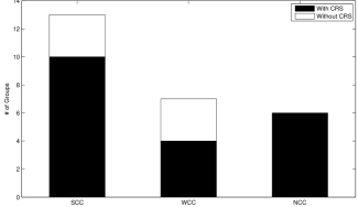
Figure 1: Fraction of SCC, WCC, and NCC groups. Shaded regions are groups with central radio sources (see Sect. 3.4.1)

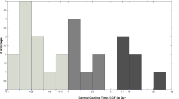
Figure 2: Histogram of central cooling time. The increasing shade of gray indicates increasing cooling time. Light grey represents SCC groups, medium grey is for WCC groups, and dark grey is for NCC groups.

3.2 Temperature profiles

The temperature profiles for all the groups, centered on the emission peak, are shown in Appendix B. We clearly see that there is no universal inner temperature profile and the magnitude of the central temperature drop, if present, varies considerably. Hudson et al. (2010) clearly showed that all SCC clusters had a central temperature drop, indicating the presence of a cool core. However, for our group sample, we find cases where despite extremely short cooling times, a central temperature rise in the innermost region is seen. This stark contrast to the properties of clusters is discussed in detail in Sect. 4.2.

3.3 Central entropy $K_{0}$

The central entropy is another parameter often used to classify CC/NCC clusters (e.g. Rafferty et al. 2008) and displays a tight correlation with the CCT (Hudson et al. 2010). This is not surprising since the cooling time, $t_{\mathrm{cool}}$, is related to the gas entropy, $K$, through the relation $t_{\mathrm{cool}}\propto K^{3/2}/T$ for pure Bremsstrahlung. We also show a histogram of the distribution of the central entropy in Fig. 3. The entropy values are given in Table 1.

The plot of the CCT and $K_{0}$ values is shown below in Fig. 4. As expected, we see an excellent correlation between the two quantities with a Spearman rank correlation coefficient of 0.99, 0.99, and 0.96 for all, SCC, and non-SCC groups respectively. A CCT of 1 Gyr corresponds to $\approx\leavevmode\nobreak\ 20\leavevmode\nobreak\ \mathrm{keV\leavevmode\nobreak\ cm}^{2}$.

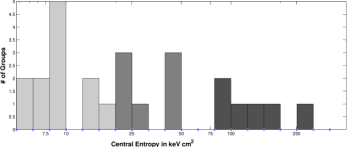
Figure 3: Histogram of the central entropy. Light grey represents SCC groups, medium grey represents WCC groups, dark grey represents NCC groups.

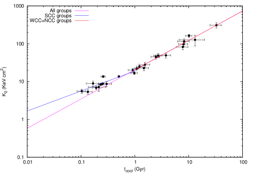
Figure 4: $K_{0}$ vs. CCT. Magenta is the best fit for all groups, blue for only SCC groups and red for WCC+NCC groups.

3.4 Radio properties

3.4.1 CRS fractions-CC/NCC dichotomy

Table 1 also lists whether or not there is a central radio source present in a group. We see that while all NCC groups have a CRS, the fractions of SCCs and WCCs containing a CRS are 77% and 57%, respectively. The overall CRS fraction for CC groups is 70%. Figure 1 shows the CRS fractions in the group sample.

3.4.2 Total radio luminosity vs. central cooling time

Mittal et al. (2009) show that there is an anti-correlation trend between the CCT and the total radio luminosity for CC clusters (correlation coefficient of $-0.63$), which breaks down for cooling times shorter than 1 Gyr.

Figure 5 shows the same plot for groups. We do not find indications of a trend between the two quantities. Here we show the best fit obtained for the CC clusters from Mittal et al. (2009) to highlight the difference between clusters and groups. The power-law fit for the CC clusters from Mittal et al. (2009) is given by:

$$L_{\mathrm{tot}}=(0.041\pm 0.016)\times(t_{\mathrm{cool}})^{-3.16\pm 0.38}\leavevmode\nobreak\ .$$ (14)

It is interesting to note that all SCC groups and most of the WCC groups show a much lower radio output than the best fit for clusters. This was first alluded to in Mittal et al. (2009), where the groups in that sample (all SCC) were clear outliers and we confirm this for the first time with a large sample of groups. We discuss this in detail in Sect. 4.3.

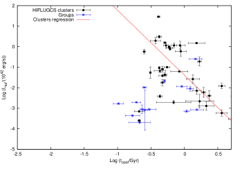
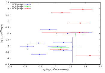
Figure 5: Left: Total radio luminosity vs. CCT with best-fit line for clusters from Mittal et al. (2009). Right: Total radio luminosity vs. mass of SMBH. The blue asterisks represent SCC groups, the green triangles represent WCC groups and the red circles represent NCC groups.

3.4.3 Total radio luminosity vs. SMBH mass

The total radio luminosity shows no trend with the SMBH mass (Fig. 5). Classifying the sample as SCC, WCC, and NCC also does not yield any discernible correlations. This is in contrast with the HIFLUGCS sample, which shows a weak correlation for the SCC clusters (correlation coefficient of 0.46). We calculate a correlation coefficient of 0.29 for all groups and 0.20 for only SCC groups. In Table 2 we present the mean SMBH masses and radio luminosities for the different CC types along with their standard errors to investigate whether different CC groups have systematically different masses and/or luminosities. We observe that the NCC groups have a systematically higher SMBH mass and radio luminosity than the SCC and WCC groups.

Table 2: Mean SMBH masses and radio luminosities for different CC groups.

Group	Mean SMBH mass ($10^{9}$ solar masses)	Mean radio luminosity ($10^{42}$ erg/s)
SCC	1.17$\pm$0.18	0.0050$\pm$0.0023
WCC	1.39$\pm$0.24	0.0034$\pm$0.0028
NCC	1.98$\pm$0.27	0.24$\pm$0.15

3.5 BCG properties

We present the scaling relation between the BCG and the cluster/group X-ray luminosity and mass in Figs. 6 and 7. The fits shown here are for a combined relation for groups and clusters. The details are summarized in Table 3. The derivation of the scatter is explained in Appendix A. We observe that most group BCGs lie above the best-fit relations. Additionally, extending the scaling relations from clusters to groups leads to a higher intrinsic scatter in most cases.

3.5.1 BCG luminosity vs. X-ray luminosity

Figure 6 shows the relation between the two quantities for both the HIFLUGCS clusters and the groups, with fits for all the members, SCC members, and non-SCC members. The correlation coefficients are 0.65, 0.79, and 0.46 for all, SCC and non-SCC systems, respectively.

It is seen that most group BCGs have a higher luminosity than expected from the derived scaling relation. The best-fit power-law relation is given by

$$\left(\frac{L_{\mathrm{BCG}}}{10^{11}L_{\odot}}\right)=c\times\left(\frac{L_{\mathrm{X}}}{10^{44}\mathrm{ergs/s}}\right)^{m}\leavevmode\nobreak\ ,$$ (15)

where $m=0.34\pm 0.03$ and $c=6.98\pm 0.16$ for all systems, $m=0.32\pm 0.03$ and $c=6.89\pm 0.20$ for SCC systems, and $m=0.43\pm 0.09$ and $c=7.01\pm 0.30$ for non-SCC systems. We observe that when the relations are extended to the group regime, there is no significant difference in slopes and normalisations for the subsets.

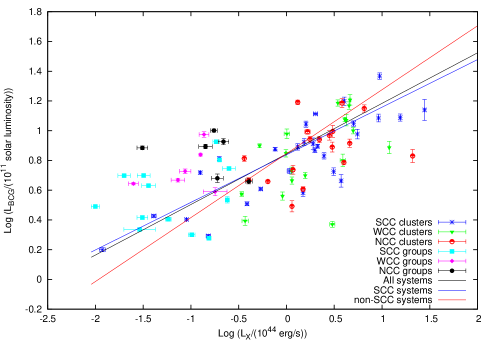
Figure 6: BCG luminosity vs. X-ray luminosity. The black line is the best fit for all systems, the blue line for only SCC systems, and the red line for non-SCC systems.

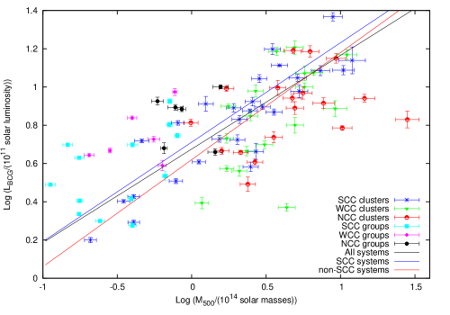
Figure 7: BCG luminosity vs. $M_{500}$. The black line is the best fit for all systems, the blue line for only SCC systems, and the red line for non-SCC systems.

3.5.2 BCG luminosity vs. $M_{500}$

Figure 7 shows that the luminosity of the BCG grows with the cluster/group mass. The correlation coefficients are 0.65, 0.86 and 0.44 for all, SCC and non-SCC systems respectively. The best fit powerlaw relation is given by:

$$\left(\frac{L_{\mathrm{BCG}}}{10^{11}L_{\odot}}\right)=c\times\left(\frac{M_{500}}{10^{14}M_{\odot}}\right)^{m}$$ (16)

where $m=0.49\pm 0.03$ and $c=4.74\pm 0.12$ for all systems, $m=0.52\pm 0.04$ and $c=5.15\pm 0.14$ for SCC systems, and $m=0.56\pm 0.08$ and $c=4.17\pm 0.03$ for non-SCC systems. We see that the normalisations for the SCC systems are around 23% higher than those for non-SCC systems.

The total mass $M_{500}$ was calculated from the virial temperature (taken from Mittal et al. 2011 and Eckmiller et al. 2011 for the clusters and groups, respectively) through the scaling relation given in Finoguenov et al. (2001):

$$\left(\frac{M_{500}}{10^{13}h^{-1}_{71}M_{\odot}}\right)=(2.5\pm 0.2)\left(\frac{kT_{\mathrm{vir}}}{1\mathrm{keV}}\right)^{1.676\pm 0.054}\leavevmode\nobreak\ .$$ (17)

Table 3: Best-fit results and scatter for BCG-cluster scaling relations: “stat” refers to statistical scatter and “int” refers to intrinsic scatter.

Category	Slope	Normalisation	$\sigma_{\mathrm{int},L_{\mathrm{X}}}$	$\sigma_{\mathrm{stat},L_{\mathrm{X}}}$	$\sigma_{\mathrm{int},L_{\mathrm{BCG}}}$	$\sigma_{\mathrm{stat},L_{\mathrm{BCG}}}$
$L_{\mathrm{X}}-L_{\mathrm{BCG}}$ Clusters	0.36$\pm$0.03	4.54$\pm$0.34	0.67	0.07	0.24	0.03
$L_{\mathrm{X}}-L_{\mathrm{BCG}}$ Clusters+Groups	0.34$\pm$0.03	6.98$\pm$0.16	0.85	0.08	0.21	0.03
$L_{\mathrm{X}}-L_{\mathrm{BCG}}$ Clusters (SCC)	0.32$\pm$0.03	5.15$\pm$0.38	0.64	0.08	0.21	0.02
$L_{\mathrm{X}}-L_{\mathrm{BCG}}$ Clusters+Groups (SCC)	0.32$\pm$0.03	6.89$\pm$0.20	0.57	0.08	0.18	0.02
$L_{\mathrm{X}}-L_{\mathrm{BCG}}$ Clusters (NSCC)	0.50$\pm$0.07	3.49$\pm$5.09	0.61	0.06	0.21	0.03
$L_{\mathrm{X}}-L_{\mathrm{BCG}}$ Clusters+Groups (NSCC)	0.43$\pm$0.09	7.01$\pm$0.30	0.64	0.07	0.29	0.03
			$\sigma_{\mathrm{int},M_{500}}$	$\sigma_{\mathrm{stat},M_{500}}$	$\sigma_{\mathrm{int},L_{\mathrm{BCG}}}$	$\sigma_{\mathrm{stat},L_{\mathrm{BCG}}}$
$M_{500}-L_{\mathrm{BCG}}$ Clusters	0.62$\pm$0.05	3.52$\pm$0.28	0.30	0.07	0.19	0.04
$M_{500}-L_{\mathrm{BCG}}$ Clusters+Groups	0.49$\pm$0.03	4.74$\pm$0.12	0.40	0.07	0.20	0.03
$M_{500}-L_{\mathrm{BCG}}$ Clusters (SCC)	0.62$\pm$0.01	4.30$\pm$0.29	0.21	0.07	0.13	0.04
$M_{500}-L_{\mathrm{BCG}}$ Clusters+Groups (SCC)	0.52$\pm$0.04	5.15$\pm$0.14	0.31	0.06	0.16	0.03
$M_{500}-L_{\mathrm{BCG}}$ Clusters (NSCC)	0.75$\pm$0.09	2.55$\pm$0.36	0.31	0.07	0.23	0.05
$M_{500}-L_{\mathrm{BCG}}$ Clusters+Groups (NSCC)	0.56$\pm$0.08	4.17$\pm$0.03	0.53	0.07	0.29	0.03

4 Discussion of results

4.1 Cool-core fraction and physical properties

A comparison between the group sample and the HIFLUGCS sample with respect to cool-core fractions is presented in Table 4.

Table 4: Comparison between observed HIFLUGCS and group sample fractions.

Point of Distinction	Group sample	HIFLUGCS
% of CC systems (SCC+WCC)	77	72
% of SCC systems	50	44
% of WCC systems	27	28
% of NCC systems	23	28

We notice that the observed fraction of CC groups is similar to that of clusters. It is worth recalling that the Malmquist bias results in higher observed CC cluster fractions and this should qualitatively extend to the group sample. Simulations have shown that SCC systems are selected preferentially because of their higher luminosity at a given temperature and correcting this bias reduces the fraction of SCC systems by about 25% (Hudson et al., 2010; Mittal et al., 2011). Eckert et al. (2011) show that the CC bias due to steeper surface brightness profiles increases for less luminous systems such as groups. Additionally, as this group sample is compiled from Chandra archives, it is statistically incomplete like most other group samples, and therefore in this case could also suffer from an archival bias, possibly resulting in a preferential selection of CC objects. These biases will be quantified with access to a complete sample (Lovisari et al. in prep.). Here, we conclude that there is no significant difference in SCC, WCC, and NCC fractions between clusters and groups.

The strong correlation between CCT and $K_{0}$ highlights that the central entropy may also serve as a good proxy to quantify the CC/NCC nature. Studies like Voit et al. (2008), Cavagnolo et al. (2009) and Rossetti et al. (2011) make use of the central entropy as the defining parameter for a CC system. This tight relation also ensures that systems defined by either parameter can be compared reasonably accurately for both clusters and groups.

4.2 Temperature profiles

A central temperature drop in the HIFLUGCS sample was a clear indication of cool gas in the centre, corroborated with short cooling times and high surface-brightnesses, particularly for the SCC clusters. We, find, however that there are some SCC groups that do not have a central temperature drop, indicating the absence of cool gas; despite having centrally peaked surface brightnesses and very short cooling times. We note that adding an additional power law to the spectral fit to account for possible low-mass X-ray binary emission does not improve the quality of the fit and also does not change this behaviour of the temperature profile.

The temperature profiles of three groups that show this feature are shown in Fig. 8.

Figure 8: Temperature profiles for NGC 6482, NGC 777 (top, both SCC), SS2B153, and NGC 1132 (bottom, SCC and WCC respectively).

The group NGC 6482 has been confirmed as a fossil group by Khosroshahi et al. (2004), who argue the shape of the temperature profile could be obtained through a steady state cooling flow solution (Fabian et al., 1984), although not ruling out heating mechanisms such as supernovae or AGN, despite the lack of a clear radio source. O’Sullivan et al. (2007) argue that SS2B is a group whose core has been partially reheated by a currently quiescent AGN in the past, and essentially that the system is currently being observed at a stage when the effects of both heating and cooling are visible. in principle, this could also be the explanation for NGC 6482 and NGC 777.

We notice that by X-ray morphology, NGC 777 and SS2B are quite similar in appearance to NGC 6482, the fossil group (Fig. 9). In the optical band, all three systems are dominated by a bright elliptical galaxy and few other galaxies. Thus, NGC 777 and SS2B could also be classified as fossil groups, but we are unable to confirm this because of the lack of magnitude information. The next question that arises is if fossil groups might be a special class of systems. In the current sample, we also have NGC 1132, another confirmed fossil group (Mulchaey & Zabludoff, 1999) with a CCT of 1.08 Gyr (making it a WCC, but it could be a SCC within errors), a CRS, and an almost flat temperature profile with a barely significant central temperature drop (Fig. 8). Thus, we speculate that fossils in general could have the features described here, i.e. a partially heated cool core. There is at least one fossil group for which this has been shown to be the case (Sun et al., 2004). It is also worth stating here that Hess et al. (2012) show that 67% of fossil groups from their sample have CRSs. However, Démoclès et al. (2010) present fossil groups that do not show a central temperature rise. These are intriguing results that we are currently investigating with a sample of fossil groups.

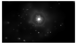
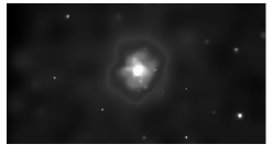
Figure 9: X-ray images of NGC 6482 (top left), NGC 777 (top right), and SS2B (bottom). The images are adaptively smoothed and exposure corrected in energy bands of 0.5-2.0 keV.

Some studies, such as Sanderson et al. (2006) and Burns et al. (2008), define a CC cluster through a central temperature drop. This has never been a problem until now as it was corroborated with short CCTs and low central entropies. We have shown, however, that this may not always be the case and caution must be exercised while using the central temperature drop as a CC diagnostic, particularly on the group regime.

4.3 AGN activity

One of the most important conclusions of the study of the HIFLUGCS sample by Mittal et al. (2009) was that as the CCT decreases, the likelihood of a cluster hosting a CRS increases. All the SCC clusters contain a CRS and this fraction drops to 45% for the NCC clusters. The fraction of groups and clusters with a CRS, classified on the basis of the CCT, is shown in Table 5. We see that, unlike clusters, the CRS fraction in groups does not scale with decreasing CCT.

Figure 5 shows that almost all CC groups have a very low radio luminosity compared to CC clusters. Quantitatively, we find that the median of the radio luminosity of the CC groups is $0.169\cdot 10^{40}$ erg/s compared to $6.21\cdot 10^{40}$ erg/s for CC clusters. This is more than an order of magnitude difference between clusters and groups. Assuming that gas cooling is responsible for the radio output of the AGN, such a low value implies that not enough gas is being accreted onto the SMBH. This could simply be due to groups having less gas than clusters to accrete onto the SMBH. We note that the gas mass for clusters is also an order of magnitude higher than that for groups (Fig. 10), making it possible that the reason for a lower radio output for groups is simply a lack of enough cooling gas, but, we also note that the correlation between the gas mass and the radio luminosity is weak (0.43 for a combined sample of clusters and groups), raising the question whether this simple explanation is sufficient to explain the low radio output. What role does star formation play here? We discuss this in Section 4.5.

The correlation coefficient between SMBH mass and radio output is very low, leading one to suspect that there is no correlation between these two quantities. This correlation has always been contentious, with studies leading to conflicting results. Franceschini et al. (1998) and Lacy et al. (2001) show a correlation between $\mathrm{L}_{\mathrm{5GHz}}$ and the mass of the SMBH, whereas Liu et al. (2006) show the absence of one. Interestingly, the NCC SMBH masses are systematically higher than the other SMBHs, raising the possibility that these objects might probably be suffering from stronger radio outbursts from larger SMBHs which might have destroyed their cool core. Though a tantalizing possibility, it could also simply be a selection effect and might have nothing to do with the CC nature of these objects.

Table 5: CRS fractions.

Point of Distinction	Group sample	HIFLUGCS sample
% of CC systems with CRS	70	75
% of NCC systems with CRS	100	45
% of WCC systems with CRS	57	67
% of SCC systems with CRS	77	100

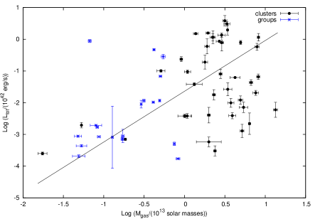
Figure 10: Total radio luminosity vs. gas mass. The gas masses presented here are within $r_{500}$ and are taken from Zhang et al. (2011) and Eckmiller et al. (2011) for clusters and groups, respectively.

4.4 BCG and cluster properties

Figures 6 and 7 show a clear trend that the BCG luminosity increases with the system mass/X-ray luminosity, but with a large amount of intrinsic scatter. Combined with the HIFLUGCS sample, there are 85 clusters and groups spanning four orders of magnitude in X-ray luminosity and three orders of magnitude in cluster mass, one of the largest comparisons carried out with CC/NCC distinction. Unlike Mittal et al. (2009), who find a segregation beween SCC clusters and non-SCC clusters in the $M_{500}-L_{\mathrm{BCG}}$ relation with different slopes and normalisations, a combined fit to groups and clusters does not yield stastically significant different slopes (although it does yield different observed normalisations). The higher normalisations and flatter slopes obtained by extending these relations suggest that groups in general have more luminous BCGs than clusters relative to $L_{\mathrm{X}}$ or $M_{500}$. Quantifying this further, we observe that $\left\langle\mathrm{log}L_{\mathrm{BCG}}-\mathrm{log}L_{\mathrm{X}}\right\rangle$ ($\left\langle\mathrm{log}L_{\mathrm{BCG}}-\mathrm{log}M_{500}\right\rangle$) is 1.7334 for groups (1.0252) vs. 0.6375 for clusters (0.3740).

To illustrate this point further, the same relations are presented again with only the fits for only groups in Fig. 11. For the complete group sample, the normalisation for the $L_{\mathrm{X}}-L_{\mathrm{BCG}}$ relation increases by more than a factor of 5 ($23.4\pm 15.2$ vs $4.54\pm 0.34$) and by more than a factor of 2 for the $M_{500}-L_{\mathrm{BCG}}$ relation ($8.39\pm 0.80$ vs $3.52\pm 0.28$) compared to that for clusters only. There are also indications that the slope is steeper, but not significantly so ($0.66\pm 0.27$ for the $L_{\mathrm{X}}-L_{\mathrm{BCG}}$ and $0.72\pm 0.10$ for the $M_{500}-L_{\mathrm{BCG}}$) relation. Assuming that the NIR luminosity is a good stellar mass proxy (e.g. Bell & de Jong 2001), all the above points hint that groups have relatively more stellar mass in their BCGs than clusters.

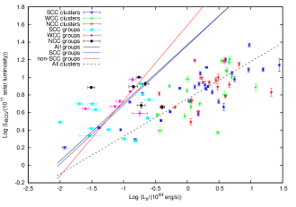
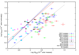
Figure 11: $L_{\mathrm{X}}-L_{\mathrm{BCG}}$ and $M_{500}-L_{\mathrm{BCG}}$ relations. The black line is the best fit for all groups, the blue line for SCC groups and the red line for non-SCC groups. The dotted line shows the fit for all clusters.

4.5 The Role of star formation

When trying to understand the relation between gas cooling and AGN feedback in groups, one cannot ignore the role of star formation. As pointed out by authors like Lagana et al. (2011), Lin et al. (2003), and Laganá et al. (2008), less massive cold clusters/groups are more prolific star forming environments. Rafferty et al. (2008) show that for groups and clusters, star formation kicks in when the central entropy is below 30 keV $\mathrm{cm}^{2}$, with the requirement that the X-ray and galaxy centroids are within 20 kpc. In our sample, all our CC BCGs are within 20 kpc of the X-ray EP, and all SCC groups and a few WCC groups have a central entropy well below the entropy limit, thus fulfilling these criteria for star formation. Hicks et al. (2010) use UV data from GALEX to show that there is a good correlation between gas cooling time and star formation rate (SFR) for CC cluster BCGs, such that the SFR increases with decreasing cooling time. Additionally, in most cases the classical mass deposition rates for our CC groups is not too high (a rough estimate yields a median of $<10\leavevmode\nobreak\ \mathrm{M}_{\odot}$/yr calculated at a radius where the cooling time is 7.7 Gyr) which means that one cannot rule out the possibility that star formation is being fueled by most of the cooling gas. This is of course a hypothesis, and confirmation of this can be provided if stronger correlations between the cooling times and star formation rates were seen for groups than for clusters. Therefore, we plan to acquire $\mathrm{H}\alpha$ data for the group BCGs to constrain SFRs.

5 Summary and conclusions

With a sample of 26 Chandra galaxy groups we have peformed a study of the ICM cooling, AGN feedback and the BCG properties on the galaxy group scale. The major results of our study are as follows.

• The group sample has similar SCC, WCC, and NCC fractions to the HIFLUGCS cluster sample.

• We find that 23% of the groups that have CCT $\leq$ 1 Gyr do not show a central temperature drop. We speculate that this could be due to a partial reheating of the cool core in the past. Additionally, we also speculate that this might be a characteristic feature of fossil groups.

• An increase in the CRS fraction with decreasing CCT is not seen, unlike for the HIFLUGCS sample. This is the first indication of differences between clusters and groups in the AGN heating/ICM cooling paradigm.

• There is no correlation seen between the CCT and the integrated radio luminosity of the CRS. We notice that CRSs for the SCC groups, in particular, have a much lower radio luminosity than clusters.

• We extend the scaling relations between $L_{\mathrm{BCG}}$ and global cluster properties ($L_{\mathrm{X}}$ and $M_{500}$) into the group regime. Most group BCGs have a BCG luminosity above the best fit and we think this may be due to a higher stellar mass content in group BCGs than in cluster BCGs, for a given $L_{\mathrm{X}}$ and $M_{500}$.

• We have speculated that star formation is a possible, effective answer to the fate of the cool gas in groups where, because of fueling star formation, not enough gas (low as it is) is being fed to the SMBH and hence the radio output of the CRSs is not as high. This could also explain why some SCC groups do not show a CRS.

In conclusion, we have demonstrated differences between clusters and groups vis-a-vis ICM cooling, AGN feedback, and BCG properties. These results lend support to the idea that groups are not simply scaled-down versions of clusters. In the future, it would be interesting to study the impact of these processes on scaling relations for galaxy groups.

Table 6: Radio data for CRS.

Cluster	$\nu$ (GHz)	Flux density (mJy)	${L}_{\mathrm{1.4GHz}}$ ($10^{32}$ erg/s/Hz)	$L_{\mathrm{tot}}10^{42}$ (erg/s)	SI of 1
A0160	$1.4^{\dagger}$	1042.8$\pm$35.7	$0.44847^{+0.0154}_{-0.0153}$	$0.4676^{+0.0147}_{-0.0276}$
	$0.408^{\mathrm{a}}$	1660$\pm$60
HCG62	$1.4^{\dagger}$	4.9$\pm$0.5	$0.000195^{+0.00002}_{-0.00002}$	$0.000205^{+0.00002}_{-0.000021}$	YES
IC1262	$1.4^{\dagger}$	87.6$\pm$6.3	$0.021156^{+0.001521}_{-0.005625}$	$0.0215^{+0.0015}_{-0.0016}$	YES
IC1633	$1.4^{\mathrm{b}}$	1.59$\pm$0.039	$0.00015891^{+0.000005}_{-0.000005}$	$0.00017142^{+0.000005}_{-0.000005}$	YES
MKW4	$1.4^{\mathrm{c}}$	2.40$\pm$0.5	$0.00213^{+0.000045}_{-0.000045}$	$0.000815^{+0.003810}_{-0.000767}$
	$4.86^{\mathrm{c}}$	0.35$\pm$0.1
MKW8	$1.4^{\dagger}$	2.54$\pm$0.1	$0.000402^{+0.000025}_{-0.000025}$	$0.000504^{+0.000088}_{-0.000031}$
	$4.86^{\mathrm{c}}$	2.09$\pm$0.15
NGC 326	$1.4^{\dagger}$	1802$\pm$59	${0.85239}^{+0.0279}_{-0.0279}$	${0.880}^{+0.095}_{-0.101}$
	$0.174^{\spadesuit}$	5100$\pm$510
	$0.074^{\ddagger}$	12320$\pm$1440
NGC 507	$1.4^{\dagger}$	120.5$\pm$6.0	${0.007150}^{+0.000354}_{-0.000354}$	${0.008970}^{+0.001430}_{-0.002890}$
	$0.074^{\ddagger}$	3250.0$\pm$490.0
NGC 533	$1.4^{\dagger}$	28.6$\pm$1.0	${0.00183}^{+0.00006}_{-0.00006}$	${0.00194}^{+0.000069}_{-0.000066}$	YES
NGC 777	$1.4^{\dagger}$	7.0$\pm$0.5	${0.000413}^{+0.000029}_{-0.000029}$	${0.000437}^{+0.000031}_{-0.000031}$	YES
NGC 1132	$1.4^{\dagger}$	5.4$\pm$0.6	${0.000667}^{+0.00007}_{0.00007}$	${0.000717}^{+0.00008}_{0.00008}$	YES
NGC 1550	$1.4^{\dagger}$	16.6$\pm$1.6	${0.000547}^{+0.000053}_{-0.000053}$	${0.00089}^{+0.00015}_{-0.00004}$
	$2.38^{\mathrm{d}}$	8.0$\pm$3.0
	$0.074^{\ddagger}$	670.0$\pm$177.0
NGC 4936	$1.4^{\dagger}$	39.8$\pm$1.6	${0.00117}^{+0.00005}_{-0.00005}$	${0.00048}^{+0.00001}_{-0.00002}$
	$0.843^{\clubsuit}$	35.2$\pm$1.9
NGC 5129	$1.4^{\dagger}$	7.2$\pm$0.5	${0.00082}^{+0.00006}_{-0.00006}$	${0.00088}^{+0.00006}_{-0.00006}$	YES
NGC 5419	$1.4^{\dagger}$	349.2$\pm$12.2	${0.01536}^{+0.00064}_{-0.00064}$	${0.01162}^{+0.00097}_{-0.00114}$
	$0.843^{\clubsuit}$	529.3$\pm$16
	$0.074^{\ddagger}$	1580$\pm$240
NGC 6269	$1.4^{\dagger}$	50$\pm$1.9	${0.012532}^{+0.00048}_{-0.00048}$	${0.01166}^{+0.00079}_{-0.00104}$
	$0.074^{\ddagger}$	560$\pm$100
NGC 6338	$1.4^{\dagger}$	57$\pm$1.8	${0.0095806}^{+0.00030}_{-0.00030}$	${0.01034}^{+0.00033}_{-0.00033}$	YES
RXCJ2214	$1.4^{\dagger}$	1604.7$\pm$50.7	$0.24691^{+0.00780}_{-0.00780}$	$0.2530^{+0.0051}_{-0.0051}$	YES
S0463	$0.843^{\clubsuit}$	314$\pm$9.6	-	${0.0687}^{+0.0003}_{-0.0003}$	YES
SS2B	$1.4^{\dagger}$	31.9$\pm$1.4	${0.00160}^{+0.00009}_{-0.00009}$	${0.00169}^{+0.00010}_{-0.00010}$	YES

$\dagger$ NVSS-Condon et al. (1998)                   $\ddagger$ VLSS-Cohen et al. (2007)
$\spadesuit$ 4C catalog-Pilkington & Scott (1965)                   $\clubsuit$ SUMSS-Bock et al. (1999)
a Robertson & Roach (1990)                                b Hopkins et al. (2000)
c From Mittal et al. (2009), based on data from the VLA (Very Large Array) Archive
d Dressel & Condon (1978)

Appendix A Calculation of scatter

We explain the calculation of scatter given in Table 3, which is based on the weighted sample variance in the log-log plane (Arnaud et al. 2005; Mittal et al. 2011):

$$\sigma_{\mathrm{raw},\leavevmode\nobreak\ L_{\mathrm{BCG}}}^{2} = \mathrm{C}_{L_{\mathrm{BCG}}}\sum_{i=1}^{N}\frac{1}{\sigma_{i,\leavevmode\nobreak\ L_{\mathrm{BCG}}}^{2}}\left[\mathrm{lg}(L_{\mathrm{BCG_{i}}})-(\lg c+m\mathrm{lg}(L_{\mathrm{X_{i}}}))\right]^{2}$$

$$\mathrm{C}_{L_{\mathrm{BCG}}} = \frac{1}{(N-2)}\frac{N}{\sum_{i=1}^{N}(1/\sigma_{i,\leavevmode\nobreak\ L_{\mathrm{BCG}}}^{2})}\,$$

$$\sigma_{\mathrm{raw},\leavevmode\nobreak\ L_{\mathrm{X}}}^{2} = {C_{L_{\mathrm{X}}}}\sum_{i=1}^{N}\frac{1}{\sigma_{i,\leavevmode\nobreak\ L_{\mathrm{X}}}^{2}}\left[\lg(L_{\mathrm{X_{i}}})-(\lg(L_{\mathrm{BCG_{i}}})-\lg c)/m\right]^{2}$$

$$\mathrm{{C_{L_{\mathrm{X}}}}} = \frac{1}{(N-2)}\frac{N}{\sum_{i=1}^{N}(1/\sigma_{i,\leavevmode\nobreak\ L_{\mathrm{X}}}^{2})}\,$$

where ${\sigma}_{i,\leavevmode\nobreak\ L_{\mathrm{BCG}}}^{2}=(\Delta\mathrm{lg}(L_{\mathrm{BCG}_{i}}))^{2}+{m}^{2}(\Delta\mathrm{lg}(L_{\mathrm{X}_{i}}))^{2}$,

${\sigma}_{i,\leavevmode\nobreak\ L_{\mathrm{X}}}^{2}=(\Delta\mathrm{lg}(L_{\mathrm{X}_{i}}))^{2}+(\Delta\mathrm{lg}(L_{\mathrm{BCG}_{i}}))^{2}/{m}^{2}$,

Here, $N$ is the sample size, $c$ is the normalisation, $m$ is the slope and the deltas represent the errors on the quantities. The statistical scatter, $\sigma_{\mathrm{stat}}$, is estimated by calculating the root-mean-square of $\sigma_{i}$. The intrinsic scatter is given as the difference between the raw and the statistical scatters in quadrature. We simply replace $M_{500}$ in place of $L_{\mathrm{X}}$ in the formula to calculate scatter for the $M_{500}-L_{\mathrm{BCG}}$ relation.

Appendix B Temperature profiles

Figure 12: Temperature profiles of A0160 (left) and A1177 (right).

Figure 13: Temperature profiles of ESO 55 (left) and HCG 62 (right).

Figure 14: Temperature profiles of HCG 97 (left) and IC 1262 (right).

Figure 15: Temperature profiles of IC 1633 (left) and MKW 4 (right).

Figure 16: Temperature profiles of MKW 8 (left) and NGC 326 (right).

Figure 17: Temperature profiles of NGC 507 (left) and NGC 533 (right).

Figure 18: Temperature profiles of NGC 777 (left) and NGC 1132 (right).

Figure 19: Temperature profiles of NGC 1550 (left) and NGC 4325 (right).

Figure 20: Temperature profiles of NGC 4936 (left) and NGC 5129 (right).

Figure 21: Temperature profiles of NGC 5419 (left) and NGC 6269 (right).

Figure 22: Temperature profiles of NGC 6338 (left) and NGC 6482 (right).

Figure 23: Temperature profiles of RXCJ 1022 (left) and RXCJ 2214 (right).

Figure 24: Temperature profiles of S0463 (left) and SS2B (right).

Appendix C NVSS radio contours on optical images for some groups

Here, we present 1.4 GHz NVSS radio contours (green) overlaid on optical images from SAO-DSS with the EP marked (red X point). Co-ordinates are sexagesimal Right Ascension and Declination.

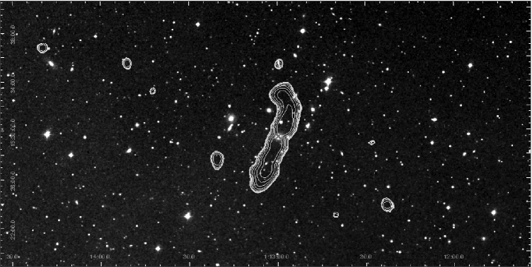
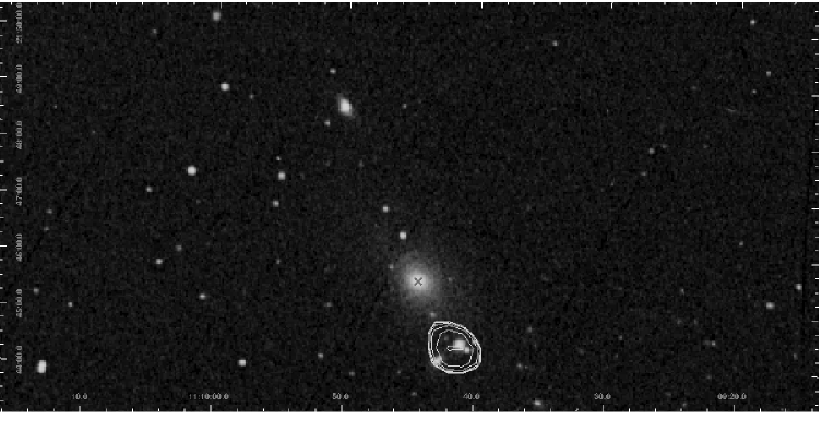
Figure 25: A0160 and A1177.

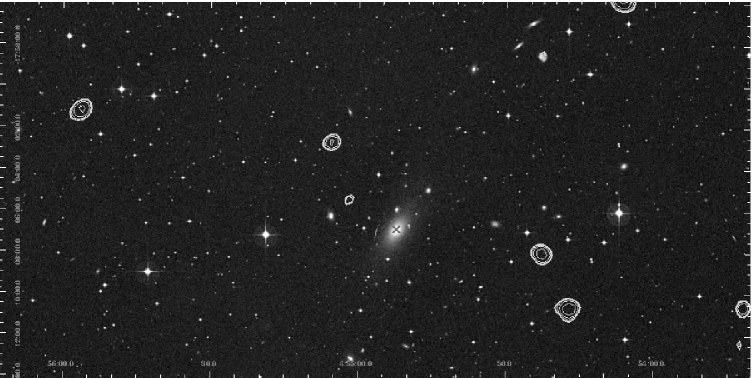
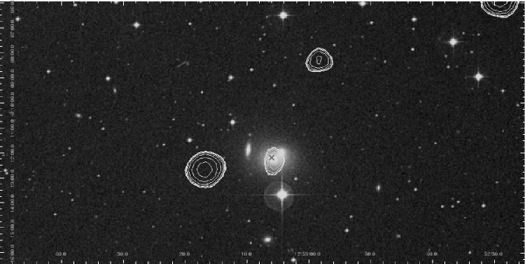
Figure 26: ESO55 and HCG62.

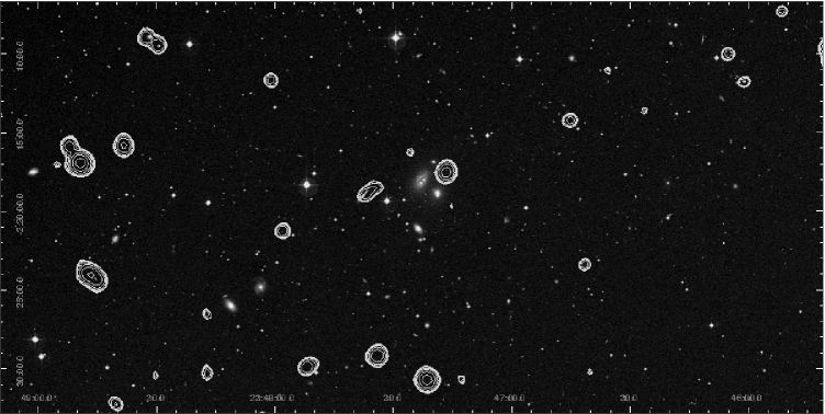
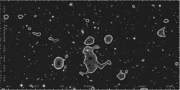
Figure 27: HCG97 and IC1262.

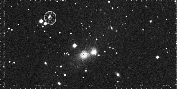
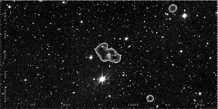
Figure 28: MKW8 and NGC326.

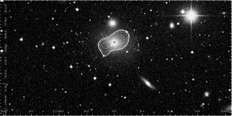
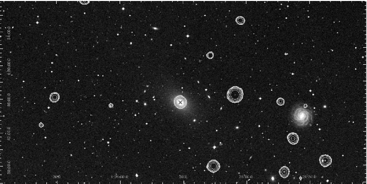
Figure 29: NGC507 and NGC533.

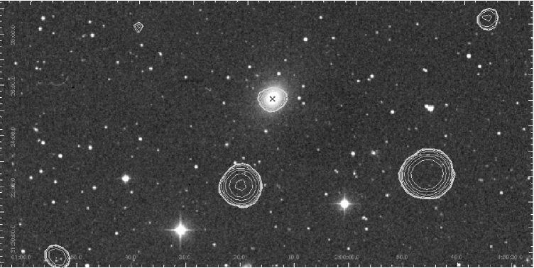
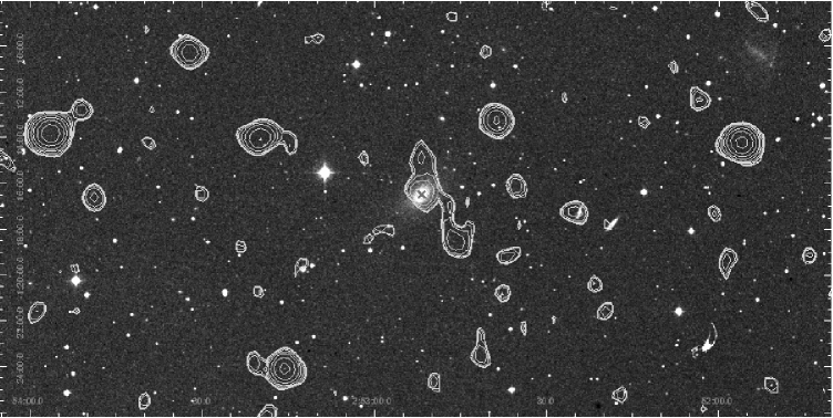
Figure 30: NGC777 and NGC1132.

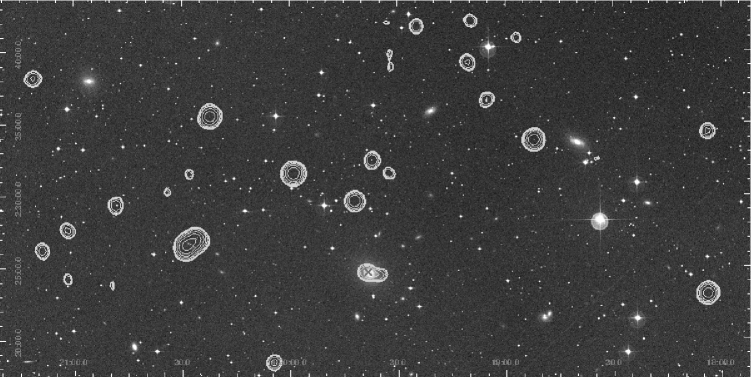
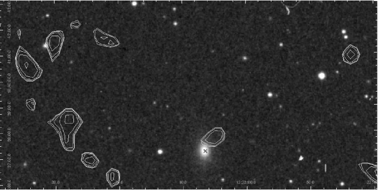
Figure 31: NGC1550 and NGC4325.

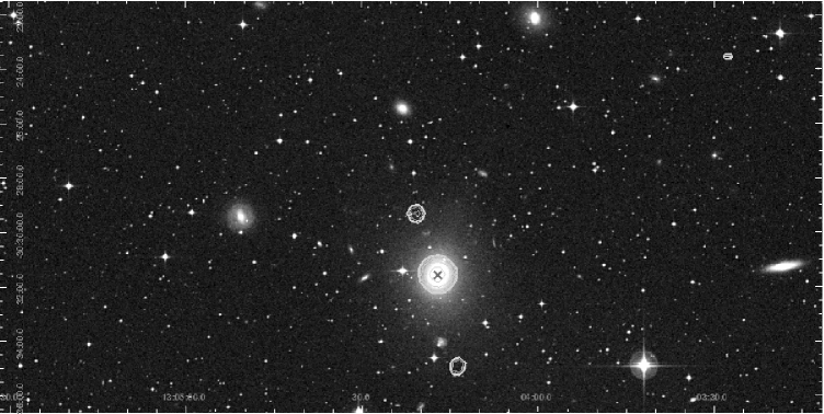
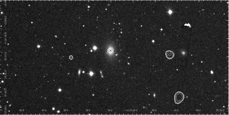
Figure 32: NGC4936 and NGC5129.

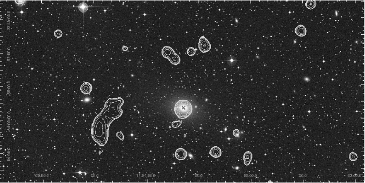
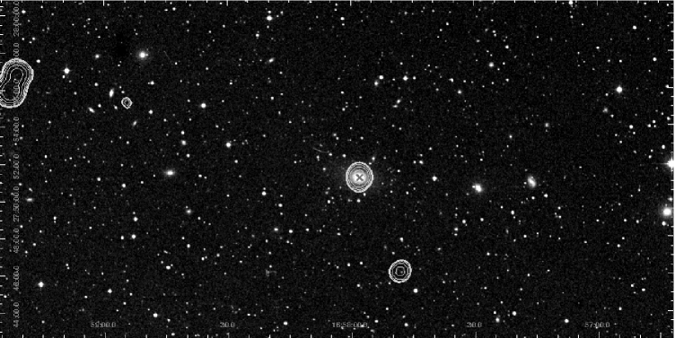
Figure 33: NGC5419 and NGC6269.

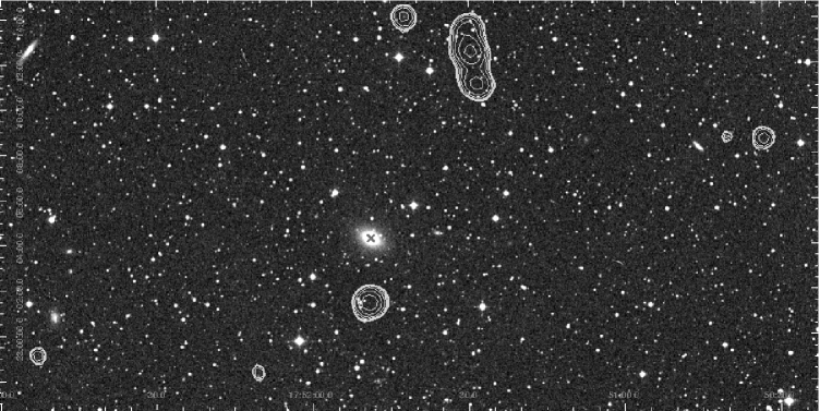
Figure 34: NGC6338 and NGC6482.

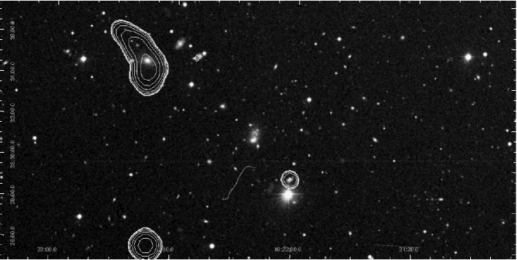
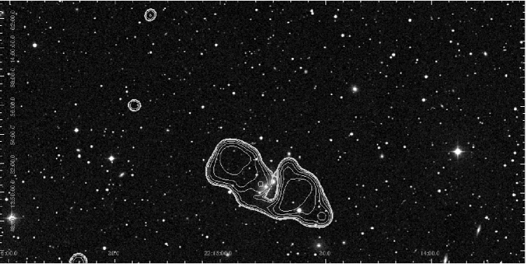
Figure 35: RXCJ1022 and RXCJ2214.

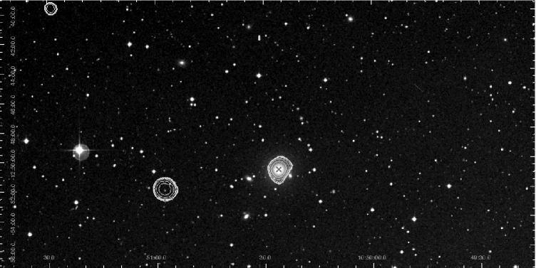
Figure 36: SS2B.