Generalized Moment Method for Gap Estimation
and Quantum Monte Carlo Level Spectroscopy

Abstract

We formulate a convergent sequence for the energy gap estimation in the worldline quantum Monte Carlo method. The ambiguity left in the conventional gap calculation for quantum systems is eliminated. Our estimation will be unbiased in the low-temperature limit and also the error bar is reliably estimated. The level spectroscopy from quantum Monte Carlo data is developed as an application of the unbiased gap estimation. From the spectral analysis, we precisely determine the Kosterlitz-Thouless quantum phase-transition point of the spin-Peierls model. It is established that the quantum phonon with a finite frequency is essential to the critical theory governed by the antiadiabatic limit, i.e., the $k=1$ SU(2) Wess-Zumino-Witten model.

The excitation gap is one of the most fundamental physical quantities in quantum systems. The Haldane phase and the $Z_{2}$ topological phase are characterized by the topologically protected gap Hasan and Kane (2010). Recently the existence of gapful/gapless quantum spin-liquid phases has been discussed in frustrated spin systems Balents (2010). Not only in the gapful but also critical phases, the system-size dependence of the excitation gap is useful for the analysis of the quantum phase transition Nomura (1995). Particularly, the energy gap $\Delta$ in the conformal quantum phases scales as $\Delta\propto xv/L$, apart from possible logarithmic correction, where $L$ is the system size, $x$ is the scaling dimension, and $v$ is the velocity appearing in the conformal field theory Cardy (1996); *FrancescoMS1997. An unbiased gap calculation thus allows for extracting the universal properties of the critical phases from finite-size data.

The gap estimation for large systems is not trivial. For small systems, it is possible to calculate the gap by the exact diagonalization method. The reachable system size is, however, strongly limited because of the explosion of required memory size and computation time. The density matrix renormalization group (DMRG) method White (1992) works well for many one-dimensional systems, but it becomes less effective in gapless or degenerated phases. In the meanwhile, the quantum Monte Carlo (QMC) method based on the worldline representation is a powerful method for various strongly correlated systems without dimensional restriction Kawashima and Harada (2004); *Sandvik2010. In previous QMC calculations Yamamoto (1995); *MengLWAM2010, the gap is extracted by the fitting of the correlation function; the tail of the exponential function is estimated as a fitting parameter [see Eq. (1) below]. Here we encounter a trade-off between the systematic error and the statistical error. The lower the temperature is in a QMC simulation, the smaller the systematic error becomes but the larger the statistical error does. It is because the correlation in long imaginary time has an exponentially small absolute value. Since in practice we do not have a prior knowledge for the optimal temperature and the range of imaginary time where the correlation function follows the asymptotic form, a choice of data necessarily introduces some bias in the fitting procedure. Our purpose in the present paper is to establish a versatile and unbiased gap-estimation procedure free from an ambiguous fitting.

In the meanwhile, the recently advanced technology has allowed for quantum simulators that can realize ideal quantum many-body systems Blatt and Roos (2012); *GeorgescuAN2014. In particular, the quantum phonon effect of trapped ions has caught a great deal of attention, which provides rich physics and engineering, e.g., spin frustration Bermudez et al. (2011), long-range spin interaction Britton et al. (2012), phonon superfluids Porras and Cirac (2004), quantum gates Zhu et al. (2006), etc. As an application of the present gap-estimation method, we will elucidate the quantum phase transition of the spin system coupled with quantum phonons, which is called the spin-Peierls transition Cross and Fisher (1979); Kuboki and Fukuyama (1987); Caron and Moukouri (1996); Wellein et al. (1998); Weiße et al. (1999, 2006); Citro et al. (2005) and is accessible in the ion system Bermudez and Plenio (2012). The level spectroscopy Nomura (1995) from Monte Carlo data is developed to overcome the difficulty of the [Kosterlitz-Thouless (KT)] transition that makes the conventional approaches ineffective. We establish that the quantum phonon effect is essential to the spin-Peierls system and its critical phenomena.

The spectral information of a quantum system described by a Hamiltonian $H$ is encoded in the imaginary time (dynamical) correlation function:

$$C(\tau) = \langle\hat{O}(\tau)\hat{O}^{\dagger}\rangle=\frac{1}{Z}{\rm tr}\left[e^{\tau H}\hat{O}e^{-\tau H}\hat{O}^{\dagger}e^{-\beta H}\right]$$ (1)

$$= \frac{1}{Z}\sum_{\ell,\ell^{\prime}}b_{\ell,\ell^{\prime}}e^{-\tau(E_{\ell}-E_{\ell^{\prime}})}e^{-\beta E_{\ell^{\prime}}}$$

$$\rightarrow \sum_{\ell\geq 1}b_{\ell}e^{-\tau(E_{\ell}-E_{0})}\quad(\beta\rightarrow\infty),$$

where $\hat{O}$ is a chosen operator, $Z$ is the partition function and $\beta=1/T$ is the inverse temperature. Also, $\{|\ell\rangle\}$ is the complete orthogonal set of eigenstates, $E_{\ell}$ is the associated eigenenergy, $b_{\ell,\ell^{\prime}}=|\langle\ell^{\prime}|\hat{O}|\ell\rangle|^{2}$, and $b_{\ell}=b_{\ell,0}$, where the ground state is $|0\rangle$, the first excited state is $|1\rangle$, and so are the higher excited states, respectively. We assume $\mbox{$\hat{O}$}|0\rangle\neq 0$, $\langle 0|\mbox{$\hat{O}$}|0\rangle=0$, and $E_{\ell}>E_{0}$ ($\ell\geq 1$), i.e., the ground state is certainly excited by the operator and the gap is finite. The latter is the case for finite-size systems even if the ground state is degenerated in the thermodynamic limit.

Here, let us consider the moment of the imaginary time correlation function Todo (2006):

$$I_{k}=\frac{1}{k!}\int_{0}^{\infty}\tau^{k}C(\tau)d\tau=\sum_{\ell\geq 1}\frac{b_{\ell}}{\Delta_{\ell}^{k+1}}\qquad(k\geq 0),$$ (2)

where $\Delta_{\ell}\equiv\Delta_{\ell,0}$, and $\Delta_{\ell,\ell^{\prime}}=E_{\ell}-E_{\ell^{\prime}}$. The higher moment will be dominated by the contribution from the first excitation gap as $I_{k}\sim b_{1}/\Delta_{1}^{k+1}$ because $\Delta_{1}<\Delta_{2}<\Delta_{3}<\cdots$. Then we can see a useful limit, $(I_{k}/I_{k+m})^{1/m}\rightarrow\Delta_{1}$ ($k\rightarrow\infty$) $\forall m\in{\mathbf{N}}$. However, we cannot use the moment directly in finite-temperature simulations. It is because the correlation function is periodic for bosons or anti-periodic for fermions and the moment is not well defined. Then the Fourier series can be exploited instead. Let us think of the bosonic case because we will investigate spin excitation. The Fourier component of the correlation function at a Matsubara frequency $\omega_{j}=2\pi j/\beta$ $(j\in{\mathbf{Z}})$ is expressed as

$$\tilde{C}(\omega_{j})=\int_{0}^{\beta}C(\tau)e^{i\tau\omega_{j}}d\tau$$ (3)

$$=\left\{\begin{array}[]{l}\displaystyle\frac{1}{Z}\sum_{\ell,\ell^{\prime}}\frac{g_{\ell,\ell^{\prime}}\Delta_{\ell,\ell^{\prime}}}{\Delta_{\ell,\ell^{\prime}}^{2}+\omega_{j}^{2}}\quad(\omega_{j}\neq 0)\\ \displaystyle\frac{1}{Z}\{\sum_{E_{\ell}\neq E_{\ell^{\prime}}}\frac{g_{\ell,\ell^{\prime}}}{\Delta_{\ell,\ell^{\prime}}}+\sum_{E_{\ell}=E_{\ell^{\prime}}}b_{\ell,\ell^{\prime}}e^{-\beta E_{\ell}}\beta\}\quad(\omega_{j}=0),\end{array}\right.$$

where $g_{\ell,\ell^{\prime}}=b_{\ell,\ell^{\prime}}(e^{-\beta E_{\ell^{\prime}}}-e^{-\beta E_{\ell}})$. In many simulations, the so-called second moment Cooper et al. (1982) is used as the lowest-order gap estimator:

$$\hskip-10.00002pt\hat{\Delta}_{(1,\beta)}=\omega_{1}\sqrt{\frac{\tilde{C}(\omega_{1})}{\tilde{C}(\omega_{0})-\tilde{C}(\omega_{1})}}\ \rightarrow\ \sqrt{\frac{I_{0}}{I_{2}}}\quad(\beta\rightarrow\infty).$$ (6)

Interestingly, this estimator will be the ratio of the zeroth and the second moment in the low-temperature limit. We have to take notice of the systematic error carefully. The error remains even in $\beta\rightarrow\infty$ as

$$\frac{\hat{\Delta}_{(1,\beta)}}{\Delta_{1}}\rightarrow\ 1+\frac{1}{2}\sum_{\ell>1}\left[\frac{b_{\ell}}{b_{1}}\frac{\Delta_{1}}{\Delta_{\ell}}+O\left(\left(\frac{\Delta_{1}}{\Delta_{\ell}}\right)^{2}\right)\right],$$ (7)

which is typically a few percent of $\Delta_{1}$ Todo and Kato (2001). This correction hampers proper identification of the universality class in the level spectroscopy analysis as we will see below.

Our main idea in the present paper is to construct a sequence of gap estimators that converges to a ratio of higher-order moments in the low-temperature limit. We will consider an estimator that has a correction of $O((\Delta_{1}/\Delta_{\ell})^{2n-1})$. Let us expand Eq. (3) in powers of ($1/\beta\Delta_{\ell,\ell^{\prime}}$) and make a linear combination of Fourier components so that the lowest orders cancel; $(-1)^{n}\sum_{k=0}^{n}x_{n,k}\tilde{C}(\omega_{k})=\sum_{\ell,\ell^{\prime}}g_{\ell,\ell^{\prime}}\omega_{1}^{2n}\Delta_{\ell,\ell^{\prime}}^{-(2n+1)}/Z+O(\beta^{-(2n+2)}\Delta_{\ell,\ell^{\prime}}^{-(2n+3)})$ with coefficients $x_{n,k}$. It will be dominated by the smallest gap $\Delta_{1}$ in $\beta\rightarrow\infty$ and $n\rightarrow\infty$. The coefficients $x_{n,k}$ satisfy the following equations: $\sum_{k=0}^{n}x_{n,k}k^{2m}=\delta_{m,n}$ $(0\leq m\leq n)$, where $\delta_{mn}$ is the Kronecker delta. They are exactly solved for by the formula of the inverse of Vandermonde’s matrix Neagoe (1996). We can also show $(-1)^{n-1}\sum_{k=0}^{n}k^{2}x_{n,k}\tilde{C}(\omega_{k})=\sum_{\ell,\ell^{\prime}}g_{\ell,\ell^{\prime}}\omega_{1}^{2(n-1)}\Delta_{\ell,\ell^{\prime}}^{-(2n-1)}/Z+O(\beta^{-2n}\Delta_{\ell,\ell^{\prime}}^{-(2n+1)})$ by using the same $x_{n,k}$. Then, a sequence of the higher-order estimators is derived as

$$\hat{\Delta}_{(n,\beta)} =\omega_{1}\sqrt{-\left.\sum_{k=0}^{n}k^{2}x_{n,k}\tilde{C}(\omega_{k})\right/\sum_{k=0}^{n}x_{n,k}\tilde{C}(\omega_{k})}$$ (8)

with $x_{n,k}=1/\prod_{j=0,j\neq k}^{n}(k+j)(k-j)$. Importantly, $\hat{\Delta}_{(n,\beta)}\rightarrow\sqrt{I_{2(n-1)}/I_{2n}}\quad(\beta\rightarrow\infty)$, and the systematic error is expressed as

$$\hskip-10.00002pt\frac{\hat{\Delta}_{(n,\beta)}}{\Delta_{1}}\rightarrow 1+\frac{1}{2}\sum_{\ell>1}\left[\frac{b_{\ell}}{b_{1}}\left(\frac{\Delta_{1}}{\Delta_{\ell}}\right)^{2n-1}\!\!\!\!\!\!\!\!\!+O\left(\left(\frac{\Delta_{1}}{\Delta_{\ell}}\right)^{2n}\right)\right].$$ (9)

Note that $I_{k}$ can be achieved only for even-numbered $k$ since $\tilde{C}(\omega_{j})$ is real. As examples, $(x_{2,0},x_{2,1},x_{2,2})=(\frac{1}{4},-\frac{1}{3},\frac{1}{12})$ for $n=2$ Todo and Kato (2001), and $(x_{3,0},x_{3,1},x_{3,2},x_{3,3})=(-\frac{1}{36},\frac{1}{24},-\frac{1}{60},\frac{1}{360})$ for $n=3$. We have analytically written down the bias of the gap estimator (8) and shown the following remarkable property:

$$\lim_{n\rightarrow\infty}\lim_{\beta\rightarrow\infty}\hat{\Delta}_{(n,\beta)}=\lim_{\beta\rightarrow\infty}\lim_{n\rightarrow\infty}\hat{\Delta}_{(n,\beta)}=\Delta_{1}.$$ (10)

That is, these two limits are interchangeable (see the Supplemental Material  for details). This important property makes our gap estimation greatly robust. Note that the present approach works also in the stochastic series expansion QMC method by the time generation Sandvik et al. (1997).

Our generalized gap estimator is applicable to any quantum system. As an example, we will show an application with the level spectroscopy to the following one-dimensional $S=1/2$ spin-Peierls model:

$$H=\sum_{r}(1+\sqrt{\frac{\omega\,\lambda}{2}}(a_{r}+a_{r}^{\dagger}))S_{r+1}\cdot S_{r}+\sum_{r}\omega a_{r}^{\dagger}a_{r},$$ (11)

where $\omega$ is a dispersionless phonon frequency, $\lambda$ is a spin-phonon coupling constant, $S_{r}$ is the spin-$\frac{1}{2}$ operator, $a_{r}$ and $a_{r}^{\dagger}$ are the annihilation and creation operator of the soft-core bosons (phonons) at site $r$, respectively. This spin-Peierls model has been investigated in the adiabatic limit ($\omega\rightarrow 0$) Cross and Fisher (1979), from the antiadiabatic limit ($\omega\rightarrow\infty$) Kuboki and Fukuyama (1987); Wellein et al. (1998); Weiße et al. (1999); Caron and Moukouri (1996); Weiße et al. (2006); Pearson et al. (2010); Sandvik and Campbell (1999), and in its crossover Citro et al. (2005). The relevance of the present model to real materials, such as CuGeO₃ Hase et al. (1993), has been discussed Uhrig and Schulz (1996). The model is expected to exhibit a KT-type quantum phase transition between the Tomonaga-Luttinger (TL) liquid phase and the dimer phase at a finite spin-phonon coupling Caron and Moukouri (1996); Citro et al. (2005), which is absent when either spin or phonon is classically treated Cross and Fisher (1979). The realization of the quantum phase transition was recently proposed in the trapped ion system Bermudez and Plenio (2012).

It is difficult to precisely locate the transition point by the conventional analyses. The huge Hilbert space with the soft-core bosons hinders the sufficient-size calculation by the diagonalization method Wellein et al. (1998). The effective spin-model approach by the perturbation Kuboki and Fukuyama (1987) or the unitary transformation Weiße et al. (1999) does not take into account all marginal terms, e.g., the 4-spin and 6-spin interactions examined in Ref. Tang and Sandvik (2011). As for the DMRG method, it needs an additional symmetry breaking term, which blurs the phase transition point, in the degenerated phase Pearson et al. (2010). In addition, the method has difficulty in precise calculation of the relevant quantities, such as the central charge, around an essential singularity Chen et al. (2013). Also, the previous QMC approach Sandvik and Campbell (1999) suffers from the exponential divergence of the correlation length and the logarithmic correction around the KT transition point. These difficulties mentioned above can be overcome by employing the level spectroscopy method Nomura (1995); Tzeng (2012) combined with our precise gap estimation. In the TL liquid phase, the both of triplet and singlet excitation are gapless in the thermodynamic limit, but the lowest excited state of finite-size systems is the triplet because of the logarithmic correction Affleck et al. (1989); *SinghFS1989; *GiamarchiS1989; *Eggert1996. In the dimer phase, on the other hand, the first excited state is the singlet for finite-size systems. It forms the degenerated ground states eventually in the thermodynamic limit. Thus the excitation gaps of the triplet and singlet excitation intersect at a spin-phonon coupling for finite-size systems. The transition point can be efficiently extrapolated from the gap-crossing points Nomura (1995).

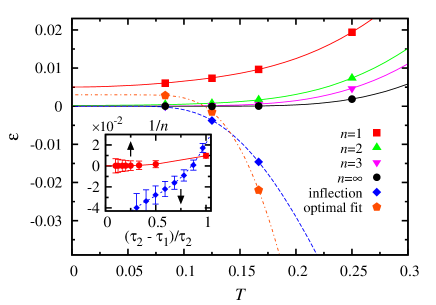
Figure 1: Triplet-gap estimation (relative) error of our estimators (8) ($n=1,2,3,\infty$), the inflection-point value of $-d\log C(\tau)/d\tau$, and the optimal fit (defined in the main text) for the spin-Peierls model (11) with $L=4$, $\omega=4$, $\lambda=1/2$, $D=4$, which has $\Delta_{1}\simeq 1.111388$. The inset shows the $n$ dependence of the gap estimate (circles) for $1\leq n\leq 10$ and the $\tau_{1}$ dependence of the $\log C(\tau)$ linear-fit result (diamonds) for $\tau_{1}\leq\tau\leq\tau_{2}$ with $\tau_{2}=\beta/4$, calculated from $2^{20}(\sim 10^{6})$ Monte Carlo steps at $\beta=6$.

We used the continuous-time worldline representation Beard and Wiese (1996); Sandvik et al. (1997) and the worm (directed-loop) algorithm Prokof’ev et al. (1998); *SyljuasenS2002 in the QMC method. Thanks to the exponential form of the diagonal operators, our simulation is free from an occupation-number cutoff of the soft-core bosons. The Fourier components of the correlation function (3) are directly calculated during the simulation. The worm-scattering probability is optimized in rejection (bounce) rate by breaking the detailed balance Suwa and Todo (2010). The boundary condition was periodic in the space and time directions. More than $2^{25}$($\simeq 3.4\times 10^{7}$) Monte Carlo samples were taken in total after $2^{18}$($\simeq 2.6\times 10^{5}$) thermalization steps. The error bar of the gap estimates is calculated by the jackknife analysis Berg (2004).

First, the convergence of our gap estimate was tested for $L=4$, $\omega=4$, $\lambda=1/2$, where $L$ is the system size. We set $\omega$ here is fairly larger than the actual spin gap because this condition is satisfied for large systems in the relevant spin-phonon coupling region. The boson occupation number cutoff $D$ was set to 4 only in this test for comparing with the diagonalization result. Fig. 1 shows the calculated triplet-gap estimation errors, where $\mbox{$\hat{O}$}=\sum_{r}S^{z}_{r}e^{i\pi r}$ is used in the dynamical correlation function. We compared the gap estimators (8) to the previous approach Yamamoto (1995); *MengLWAM2010 where the first gap is estimated as $-d\log C(\tau)/d\tau$ from the asymptotic form (1). The derivative will show a plateau at the gap value in an appropriate $\tau$ region. When $\beta(=1/T)$ is not large enough, however, the plateau is indistinct. Then the inflection point could be used, but it is hard to estimate in practice (here we calculated it by longer QMC simulation for comparison). As an another practical and reasonable gap estimation, we test a linear fit of $\log C(\tau)$ for $\tau_{1}\leq\tau\leq\tau_{2}$, where we fix $\tau_{2}=\beta/4$. The inset of Fig. 1 shows the feasible convergence of the gap estimate in $n$ and the difficulty of finding appropriate $\tau_{1}$ for the linear fit. The function $\log C(\tau)$ is poorly fitted to a linear form at small $\tau_{1}$, while it has larger statistical error at large $\tau_{1}$. Then the gap error resulting from the linear regression takes a minimum value at optimal $\tau^{*}_{1}$, which we call “optimal fit.” Even though it seems reasonable, the optimal fit underestimates the gap at $\beta=6,8$ and overestimates it at $\beta=12$ as shown in the main panel of the figure. Meanwhile, the second-moment estimator ($n=1$) has a non-negligible bias even in $T\rightarrow 0$ as expected from Eq. (7). The estimate with large enough $n$ (we call it the $n=\infty$ estimate hereafter), on the other hand, exponentially converges to the exact value as the temperature decreases Note (1). The bias convergence is much faster than that of the inflection point (one of the best estimates from the fitting approach). Moreover, the higher-order estimator provides a reliable error bar, while the optimal fit significantly underestimates it Note (1). Therefore, our approach is more precise and straightforward than the fitting approach. In the present study, we have used a simple recipe to optimize $n$ and $\beta$, minimizing both the systematic and the statistical error Note (1).

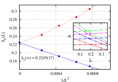
Figure 2: Convergence of the gap-crossing point (circles) between the triplet and the singlet excitation for $L=36,40,48,64$, together with the crossing point of the spin susceptibility (diamonds) between $\chi_{s}(L)/L$ and $\chi_{s}(L/2)/(L/2)$. The spin-phonon coupling dependence of the gaps is shown in the inset for each $L$. The dashed line is the fitting curve with $\lambda_{\rm c}(\infty)$ fixed, which results in large $\chi^{2}/$dof $\approx 5.0$. The statistical errors are smaller than the symbol size.

The scaling of the gap-crossing point for the spin-Peierls model between the triplet and singlet excitation is shown in Fig. 2. For the singlet excitation gap, we used $\mbox{$\hat{O}$}=\sum_{r}S_{r}\cdot S_{r+1}e^{i\pi r}$. The bare excitation phonon gap was set to $\omega=1/4$ for the comparison with the previous result Sandvik and Campbell (1999). The transition point $\lambda_{\rm c}=0.2245(17)$ in the thermodynamic limit was extrapolated without logarithmic correction, which is much more precise than the previous estimate, $0.176<\lambda_{\rm c}<0.23$ Sandvik and Campbell (1999) in our notation. Also the spin susceptibility $\chi_{s}=\int_{0}^{\beta}\sum_{r}\langle S^{z}_{r}(\tau)S^{z}_{0}\rangle e^{i\pi r}d\tau$ could be used for finding the transition point (Fig. 2). Nevertheless, the gap-crossing point provides the much more reliable extrapolation with $1/L^{2}$ correction from irrelevant fields Nomura (1995), while the susceptibility is likely to have some more complicated corrections.

We have also calculated the velocity, the central charge, and the scaling dimensions at the transition point, fixing $\lambda=0.2245$. The velocity $v=1.485(8)$ was calculated from the scaling form $v(L)=\Delta_{k_{1}}/k_{1}=v+a/L^{2}+b/L^{4}+o(1/L^{4})$, where $\Delta_{k_{1}}$ is the triplet gap at $k_{1}=2\pi/L$, $a$ and $b$ are non-universal constants. The central charge $c=0.987(13)$ was obtained from the finite-size correction Affleck et al. (1989), $E_{0}(L)=E_{0}-\pi vc/6L+o(1/L)$. The scaling dimension corresponding to the triplet or singlet excitation was calculated from the relation $x(L)=L\Delta_{\pi}/2\pi v$, where $\Delta_{\pi}$ is the lowest (triplet or singlet) excitation gap at $k=\pi$. As shown in Fig. 3, the $n=\infty$ estimates converged to $x_{S=1}=0.502(3)$ and $x_{S=0}=0.499(3)$ without logarithmic correction as expected only at the transition point Nomura (1995). Hence we conclude that this transition point is described by the $k=1$ SU(2) Wess-Zumino-Witten model Witten (1984) with $c=1$ and $x=1/2$. On the other hand, the second-moment estimates ($n=1$) failed to approach 1/2 as seen in Fig. 3. This identification of the critical theory clearly demonstrates the importance of the higher-order estimator. The present study non-trivially clarified that the critical theory at the transition point of the spin-Peierls model with a finite phonon frequency coincides with that in the antiadiabatic limit ($\omega\rightarrow\infty$) where the effective spin model is the frustrated $J_{1}$-$J_{2}$ chain Nomura (1995). Our result strongly indicates that the quantum phonon effect is relevant to the spin-Peierls system in the sense that it necessarily triggers the universal KT phase transition.

Figure 3: System-size dependence of the scaling dimension corresponding to the triplet or the singlet excitation at the transition point ($\lambda=0.2245$), calculated from the second-moment ($n=1$) or the $n=\infty$ gap estimate.

In conclusion, we have presented the generalized moment method for the gap estimation. The advantages of our method over the previous approaches are as follows: the unbiased estimation [Eq. (10)], the absence of ambiguous procedure, the faster convergence w.r.t. the temperature, and the reliable error-bar estimation. We emphasize that our approach is generally applicable to any quantum system. The QMC level spectroscopy was demonstrated, for the first time, for the KT transition in the spin-Peierls model. This spectral analysis will likely work in various systems including most conformal phases. We elucidated that the quantum phonon effect is relevant to the critical theory of the spin-phonon system, which is expected to be universal in many kinds of one-dimensional systems, e.g., (spinless) fermion-phonon systems, by virtue of the well-established transformations. The clarified quantum phase transition and the criticality would be directly observed in the quantum simulator Bermudez and Plenio (2012).

The authors are grateful to Anders W. Sandvik, Thomas C. Lang, and Hiroshi Ueda for the valuable discussion. The most simulations in the present paper were done by using the facility of the Supercomputer Center, Institute for Solid State Physics, University of Tokyo. We also used the computational resources at the Institute for Information Management and Communication, Kyoto University and Computing and Communications Center, Kyushu University through the HPCI System Research Project (No. hp140204, hp140162). The simulation code has been developed based on the ALPS library Bauer et al. (2011). The authors acknowledge the support by KAKENHI (No. 23540438, 26400384) from JSPS and CMSI in SPIRE from MEXT, Japan. HS is supported by the JSPS Postdoctoral Fellowships for Research Abroad.

Supplemental Material: Generalized Moment Method for Gap Estimation
and Quantum Monte Carlo Level Spectroscopy

I Systematic error of higher-order gap estimate

We provide here the detailed form of the bias of the gap estimator (8) and its limiting form in $n\rightarrow\infty$ and $\beta\rightarrow\infty$. The gap estimator is rewritten as

$$\hat{\Delta}_{(n,\beta)}=\sqrt{\frac{\displaystyle\sum_{E_{\ell}\neq E_{\ell^{\prime}}}g_{\ell,\ell^{\prime}}\Delta_{\ell,\ell^{\prime}}\prod_{j=1}^{n}\frac{1}{\Delta^{2}_{\ell,\ell^{\prime}}+\omega_{j}^{2}}}{\displaystyle\sum_{E_{\ell}\neq E_{\ell^{\prime}}}\frac{g_{\ell,\ell^{\prime}}}{\Delta_{\ell,\ell^{\prime}}}\prod_{j=1}^{n}\frac{1}{\Delta_{\ell,\ell^{\prime}}^{2}+\omega_{j}^{2}}+\sum_{E_{\ell}=E_{\ell^{\prime}}}b_{\ell,\ell^{\prime}}\beta e^{-\beta E_{\ell}}\prod_{j=1}^{n}\frac{1}{\omega_{j}^{2}}}}.$$ (S1)

In the equation, as the reminder of the definitions, $\Delta_{\ell,\ell^{\prime}}=E_{\ell}-E_{\ell^{\prime}}$, $b_{\ell,\ell^{\prime}}=|\langle\ell^{\prime}|\hat{O}|\ell\rangle|^{2}$, $g_{\ell,\ell^{\prime}}=b_{\ell,\ell^{\prime}}(e^{-\beta E_{\ell^{\prime}}}-e^{-\beta E_{\ell}})$, $\omega_{j}=2\pi j/\beta$ $(j\in{\mathbf{Z}})$. Here we used the useful equations:

$$\sum_{k=0}^{n}\frac{x_{n,k}}{\Delta^{2}+\omega^{2}_{k}} =(-1)^{n}\omega^{2n}_{1}\prod_{k=0}^{n}\frac{1}{\Delta^{2}+\omega^{2}_{k}},$$ (S2)

$$\sum_{k=0}^{n}\frac{k^{2}x_{n,k}}{\Delta^{2}+\omega^{2}_{k}} =(-1)^{n-1}\omega^{2(n-1)}_{1}\prod_{k=1}^{n}\frac{1}{\Delta^{2}+\omega^{2}_{k}},$$ (S3)

where $x_{n,k}=1/\prod_{j=0,j\neq k}^{n}(k+j)(k-j)$ as defined in the main text. These equations are derived from the imposed condition on $x_{n,k}$ to cancel the lowest orders of $(1/\beta\Delta_{\ell,\ell^{\prime}})$ as explained in the main text:

$$\sum_{k=0}^{n}x_{n,k}k^{2m}=\delta_{m,n}\quad(0\leq m\leq n)\quad \Longleftrightarrow\quad\sum_{k=0}^{n}x_{n,k}\sigma_{n,m}(-k)=(-1)^{n}\delta_{m,n}\quad(0\leq m\leq n)$$ (S4)

$$\,\Longrightarrow\quad\sum_{k=1}^{n}k^{2}x_{n,k}\sigma_{n,m}(-k)=(-1)^{n-1}\delta_{m,n-1}\quad(0\leq m\leq n-1),$$ (S5)

where $\sigma_{n,m}(-k)=\sigma_{m}(0,1,2^{2},3^{2},...,(k-1)^{2},(k+1)^{2},...,n^{2})$, and $\sigma_{m}$ is the elementary symmetric polynomial of order $m$, e.g., $\sigma_{0}(a_{1},a_{2},a_{3})=1$, $\sigma_{1}(a_{1},a_{2},a_{3})=a_{1}+a_{2}+a_{3}$, $\sigma_{2}(a_{1},a_{2},a_{3})=a_{1}a_{2}+a_{2}a_{3}+a_{3}a_{1}$, $\sigma_{3}(a_{1},a_{2},a_{3})=a_{1}a_{2}a_{3}$.

The systematic error of the higher-order gap estimate is expressed as

$$\frac{\hat{\Delta}_{(n,\beta)}}{\Delta_{1}}=\sqrt{\frac{1+R_{n}(\beta)}{1+\displaystyle F_{n}(\beta)+D_{n}(\beta)}}\quad\rightarrow\quad\ 1+\frac{1}{2}\sum_{\ell>1}\left[\frac{b_{\ell}}{b_{1}}\left(\frac{\Delta_{1}}{\Delta_{\ell}}\right)^{2n-1}\!\!\!\!\!\!+O\left(\left(\frac{\Delta_{1}}{\Delta_{\ell}}\right)^{2n}\right)\right]\quad(\beta\rightarrow\infty),$$ (S6)

where

$$R_{n}(\beta) =\sum_{E_{\ell}\neq E_{\ell^{\prime}},(\ell,\ell^{\prime})\neq(1,0)}\left(\frac{g_{\ell,\ell^{\prime}}}{g_{1,0}}\right)\left(\frac{\Delta_{1}}{\Delta_{\ell,\ell^{\prime}}}\right)^{-1}h(n,\beta,\Delta_{\ell,\ell^{\prime}}),$$ (S7)

$$F_{n}(\beta) =\sum_{E_{\ell}\neq E_{\ell^{\prime}},(\ell,\ell^{\prime})\neq(1,0)}\left(\frac{g_{\ell,\ell^{\prime}}}{g_{1,0}}\right)\left(\frac{\Delta_{1}}{\Delta_{\ell,\ell^{\prime}}}\right)h(n,\beta,\Delta_{\ell,\ell^{\prime}}),$$ (S8)

$$D_{n}(\beta) =\sum_{E_{\ell}=E_{\ell^{\prime}}}\left(\frac{b_{\ell,\ell^{\prime}}}{g_{1,0}}\right)\beta\Delta_{1}\,e^{-\beta E_{\ell}}\prod_{j=1}^{n}\left(1+\frac{\Delta_{1}^{2}}{\omega_{j}^{2}}\right),$$ (S9)

$$h(n,\beta,\Delta_{\ell,\ell^{\prime}})=\prod_{j=1}^{n}\frac{\Delta^{2}_{1}+\omega^{2}_{j}}{\Delta^{2}_{\ell,\ell^{\prime}}+\omega^{2}_{j}},$$ (S10)

the summations for $F_{n}$ and $R_{n}$ are taken over $E_{\ell}\neq E_{\ell^{\prime}}$ except $(\ell,\ell^{\prime})=(1,0)$ and $(0,1)$, $D_{n}$ term comes from $x_{n,0}\,\tilde{C}(0)$, and $b_{\ell}=b_{\ell,0}$. We showed, in the main text, the limiting form: $\lim_{\beta\rightarrow\infty}\hat{\Delta}_{(n,\beta)}=\sqrt{I_{2(n-1)}/I_{2n}}$, where $I_{k}$ is the moment defined as Eq. (2). Then, $\lim_{n\rightarrow\infty}\lim_{\beta\rightarrow\infty}\hat{\Delta}_{(n,\beta)}=\Delta_{1}$ since $(I_{k}/I_{k+m})^{1/m}\rightarrow\Delta_{1}$ ($k\rightarrow\infty$) $\forall m\in{\mathbf{N}}$.

Next, let us consider the limiting form in $n\rightarrow\infty$ at a finite temperature. We use the product expansion form of the hyperbolic function: $\sinh(\pi z)=\pi z\prod_{j=1}^{\infty}(1+z^{2}/j^{2})$ with $z=\beta\Delta_{\ell,\ell^{\prime}}/2\pi$ in Eq. (S6). The finite-$n$ corrections are expressed as

$$\begin{split}\prod_{j=1}^{n}(1+z^{2}/j^{2})&\sim\frac{\sinh(\pi z)}{\pi z}\exp\left\{-z^{2}\left(\frac{1}{n+1}+\frac{1}{2(n+1)(n+2)}\right)\right\}\\ &\sim\frac{\sinh(\pi z)}{\pi z}\left[1-z^{2}\left(\frac{1}{n+1}+\frac{1}{2(n+1)(n+2)}\right)+\frac{z^{4}}{2(n+1)^{2}}\right].\end{split}$$ (S11)

Here the asymptotic expansion of the Riemann zeta function was used;

$$\sum_{k=1}^{n}\frac{1}{k^{2}}=\frac{\pi^{2}}{6}-\frac{1}{n+1}-\frac{1}{2(n+1)(n+2)}-\cdots.$$ (S12)

The limiting form is then expressed as

$$\frac{\hat{\Delta}_{(n,\beta)}}{\Delta_{1}}=\sqrt{\frac{1+\displaystyle R_{\infty}(\beta)}{1+G_{\infty}(\beta)}}+O\left(\frac{1}{n}\right),$$ (S13)

where

$$R_{\infty}(\beta) =\sum_{E_{\ell}\neq E_{\ell^{\prime}},(\ell,\ell^{\prime})\neq(1,0)}\left(\frac{b_{\ell,\ell^{\prime}}}{b_{1}}\right)\left(\frac{\Delta_{1}}{\Delta_{\ell,\ell^{\prime}}}\right)^{-2}e^{-\frac{\beta}{2}{\Delta_{\rm ex}}},$$ (S14)

$$G_{\infty}(\beta) =\sum_{(\ell,\ell^{\prime})\neq(1,0)}\left(\frac{b_{\ell,\ell^{\prime}}}{b_{1}}\right)e^{-\frac{\beta}{2}{\Delta_{\rm ex}}},$$ (S15)

and $\Delta_{\rm ex}=E_{\ell}+E_{\ell^{\prime}}-E_{1}-E_{0}$. Note that the correction terms coming from $F_{n}$ and $D_{n}$ are included in $G_{\infty}$. Then, $\lim_{\beta\rightarrow\infty}\lim_{n\rightarrow\infty}\hat{\Delta}_{(n,\beta)}=\Delta_{1}$ because $\Delta_{\rm ex}>0$. As a result, the finite-$n$ corrections are $O(1/n)$. It is attainable to confirm the convergence as shown in the inset of Fig. 1 in the main text. Furthermore, the $n=\infty$ estimate shows the exponential convergence w.r.t. the temperature, which was indeed observed for the test case in the main text (see Fig. 1).

II Asymptotic Behavior of Gap Estimate for Continuum Spectrum

The systematic error (S6) was formulated for a discrete spectrum. This is the case in finite-size quantum systems with a reasonable basis. We will show a generalization to a continuum spectrum that will be achieved in the thermodynamic limit. In practice, the crossover from the discrete to continuum case will be observed in fairly large systems. First, let us generalize the formulation of the correlation functions. They are expressed as

$$C(\tau) =\int_{-\infty}^{\infty}d\/\epsilon S(\epsilon)e^{-\tau\epsilon},$$ (S16)

$$\tilde{C}(\omega_{j}) =\int_{0}^{\beta}d\/\tau C(\tau)e^{i\tau\omega_{j}}=\frac{1}{2\pi}\int_{-\infty}^{\infty}d\/\epsilon\frac{A(\epsilon)}{\epsilon-i\omega_{j}},$$ (S17)

where $A(\epsilon)=2\pi S(\epsilon)(1-\zeta e^{-\beta\epsilon})$ is the spectral function with $\zeta=1$ (bosons or spins) or $\zeta=-1$ (fermions). The formulation of a discrete spectrum is recovered by setting

$$S(\epsilon)=\frac{1}{Z}\sum_{\ell,\ell^{\prime}}b_{\ell,\ell^{\prime}}e^{-\beta E_{\ell^{\prime}}}\delta(\epsilon-(E_{\ell}-E_{\ell^{\prime}})).$$ (S18)

Then the gap estimator (8) is generally expressed as

$$\hat{\Delta}_{(n,\beta)}=\sqrt{\frac{\displaystyle\int_{-\infty}^{\infty}d\epsilon\,A(\epsilon)\epsilon\prod_{j=1}^{n}\frac{1}{\epsilon^{2}+\omega_{j}^{2}}}{\displaystyle\int_{-\infty}^{\infty}d\epsilon\,\frac{A(\epsilon)}{\epsilon}\prod_{j=1}^{n}\frac{1}{\epsilon^{2}+\omega_{j}^{2}}}}.$$ (S19)

Let us focus on the spin case here. The integrand with $O=S_{i}^{z}$ or $S_{i}^{z}S_{j}^{z}$ ($i$ and $j$ are site indices) in Eq. (S19) is symmetric at $\epsilon=0$, so considering only for $\epsilon\geq 0$ suffices. Let us then write $A(\epsilon)=A_{+}(\epsilon)$ ($\epsilon\geq 0$). When there is a delta peak at the first gap ($b_{1}>0$) and a finite gap between the first gap ($\Delta_{1}$) and the second gap ($\Delta_{2}$), as $\Delta_{2}-\Delta_{1}>0$, the systematic error (S6) is expressed in a similar way converting the discrete summation to the corresponding integral. The asymptotic form becomes

$$\frac{\hat{\Delta}_{(\infty,\beta)}}{\Delta_{1}}=1+O\left(e^{-\frac{\beta}{2}(\Delta_{2}-\Delta_{1})}\right),$$ (S20)

$$\frac{\hat{\Delta}_{(n,\infty)}}{\Delta_{1}}=1+O\left(\left(\frac{\Delta_{1}}{\Delta_{2}}\right)^{2n-1}\right).$$ (S21)

Next let us think of the case where the system has a continuum spectrum above the lowest gap ($\Delta_{1}$). The asymptotic behaviors of the gap estimate for some typical spectral function (with $\Delta_{1}>0$ or $\Delta_{1}=0$) are summed up in Table 1. The parameter constraint for each case comes from the bounded correlation function: $C(\tau)<\infty$.

(i) $A_{+}(\epsilon)\sim(\epsilon-\Delta_{1})^{a}\theta(\epsilon-\Delta_{1})\quad(a>-1)$

When the spectrum is in a power of $\epsilon-\Delta_{1}$, the systematic error will be asymptotically $O(1/n)$ or $O(1/\beta)$; that is,

$$\hat{\Delta}_{(\infty,\beta)} \sim\sqrt{\frac{Q(a,2)}{Q(a,0)}}=\Delta_{1}\left[1+O\left(\frac{1}{\beta}\right)\right],$$ (S22)

$$\hat{\Delta}_{(n,\infty)} \sim\sqrt{\frac{T(a,2n-1)}{T(a,2n+1)}}=\Delta_{1}\left[1+O\left(\frac{1}{n}\right)\right],$$ (S23)

where

$$Q(a,m) \equiv\int_{\Delta_{1}}^{\epsilon_{M}}d\epsilon\,\frac{(\epsilon-\Delta_{1})^{a}\epsilon^{m}}{\sinh\left(\frac{\beta\epsilon}{2}\right)}\sim\int_{\Delta_{1}}^{\epsilon_{M}}d\epsilon\,2(\epsilon-\Delta_{1})^{a}\epsilon^{m}e^{-\frac{\beta\epsilon}{2}}=2^{a+2}\frac{\Delta_{1}^{m}}{\beta^{a+1}}e^{-\frac{\beta\Delta_{1}}{2}}\int_{0}^{q_{M}}dq\,q^{a}\left(1+\frac{2q}{\beta\Delta_{1}}\right)^{m}e^{-q}$$

$$=\frac{\Delta_{1}^{m}}{\beta^{a+1}}e^{-\frac{\beta\Delta_{1}}{2}}\left(Q_{0}+\frac{Q_{1}}{\beta}\right)\quad(\beta\gg 1/\Delta_{1}),$$ (S24)

$$T(a,m) \equiv\int_{\Delta_{1}}^{\epsilon_{M}}d\epsilon\,\frac{(\epsilon-\Delta_{1})^{a}}{\epsilon^{m}}=\int_{0}^{T_{M}}dt\,\frac{\Delta_{1}^{a+1-m}}{m^{a+1}}\frac{t^{a}}{(1+\frac{t}{m})^{m}}\sim\int_{0}^{T_{M}}dt\,\frac{\Delta_{1}^{a+1-m}}{m^{a+1}}\frac{t^{a}}{e^{t}(1-\frac{t^{2}}{2m})}$$

$$=\frac{\Delta_{1}^{a+1-m}}{m^{a+1}}\left(T_{0}+\frac{T_{1}}{m}\right)\quad(m\gg 1).$$ (S25)

In Eq. (S24) $q=\beta(\epsilon-\Delta_{1})/2$, in Eq. (S25) $\epsilon=(1+\frac{t}{m})\Delta_{1}$, and $\epsilon_{M},q_{M},t_{M},Q_{0},Q_{1},T_{0},T_{1}$ are constants.

Table 1: Asymptotic behavior of the gap estimate for typical continuum spectrum. In the spectral function row, $\theta(x)$ is the unit step function; it takes $0\ (x<0)$ or $1\ (x\geq 0)$.

$A_{+}(\epsilon)$	$(\epsilon-\Delta_{1})^{a}\theta(\epsilon-\Delta_{1})$ ($a>-1$)	$e^{-c/(\epsilon-\Delta_{1})^{a}}\theta(\epsilon-\Delta_{1})$ ($a,c>0$)	$\epsilon^{a}$ ($a>0$)	$e^{-c/\epsilon^{a}}$ ($a,c>0$)
$\hat{\Delta}_{(\infty,\beta)}$	$\Delta_{1}[1+O(1/\beta)]$	$\Delta_{1}[1+O(1/\beta^{\frac{1}{a+1}})]$	$\sim 1/\beta$	$\sim 1/\beta^{\frac{1}{a+1}}$
$\hat{\Delta}_{(n,\infty)}$	$\Delta_{1}[1+O(1/n)]$	$\Delta_{1}[1+O(1/n^{\frac{1}{a+1}})]$	0	$\sim 1/n^{\frac{1}{a}}$

(ii) $A_{+}(\epsilon)\sim e^{-c/(\epsilon-\Delta_{1})^{a}}\theta(\epsilon-\Delta_{1})\quad(a,c>0)$

Even when the spectral function vanishes exponentially at $\epsilon=\Delta_{1}>0$, the gap estimator will be asymptotically unbiased. The convergence becomes slower than the power-law case:

$$\hat{\Delta}_{(\infty,\beta)} \sim\sqrt{\frac{U(a,c,2)}{U(a,c,0)}}=\Delta_{1}\left[1+O\left(\frac{1}{\beta^{\frac{1}{a+1}}}\right)\right],$$ (S26)

$$\hat{\Delta}_{(n,\infty)} \sim\sqrt{\frac{V(a,c,2n-1)}{V(a,c,2n+1)}}=\Delta_{1}\left[1+O\left(\frac{1}{n^{\frac{1}{a+1}}}\right)\right],$$ (S27)

where

$$U(a,c,m) \equiv\int_{\Delta_{1}}^{\epsilon_{M}}d\epsilon\,\frac{e^{-\frac{c}{(\epsilon-\Delta_{1})^{a}}}\epsilon^{m}}{\sinh\left(\frac{\beta\epsilon}{2}\right)}=:\int_{\Delta_{1}}^{\epsilon_{M}}d\epsilon\,e^{-u_{m}(\epsilon)}\approx\sqrt{\frac{2\pi}{u^{\prime\prime}_{m}(\epsilon_{m}^{*})}}e^{-u_{m}(\epsilon_{m}^{*})}\sim\Delta_{1}^{-m}e^{-m\,\beta^{-\frac{1}{a+1}}}\quad(\beta\gg 1/\Delta_{1}),$$ (S28)

$$V(a,c,m) \equiv\int_{\Delta_{1}}^{\epsilon_{M}}d\epsilon\,e^{-\frac{c}{(\epsilon-\Delta_{1})^{a}}}\epsilon^{-m}=:\int_{\Delta_{1}}^{\epsilon_{M}}d\epsilon\,e^{-v_{m}(\epsilon)}\approx\sqrt{\frac{2\pi}{v^{\prime\prime}_{m}(\epsilon_{m}^{*})}}e^{-v_{m}(\epsilon_{m}^{*})}\sim\Delta_{1}^{-m}m^{-\frac{a+2}{2(a+1)}}e^{-m^{\frac{a}{a+1}}}\quad(m\gg 1),$$ (S29)

$u^{\prime\prime}_{m}(\epsilon)$ and $v^{\prime\prime}_{m}(\epsilon)$ are the second derivative, and the saddle-point approximation around its extremum $u^{\prime}_{m}(\epsilon_{m}^{*})=v^{\prime}_{m}(\epsilon_{m}^{*})=0$ were used, respectively.

(iii) $A_{+}(\epsilon)\sim\epsilon^{a}\quad(a>0)$

Let us consider the gapless case with a power-law form. From Eq. (S19), the estimate will diverge since the gap is actually zero, but it takes a finite value for the case of finite $\beta$:

$$\hat{\Delta}_{(n,\beta)} \sim\sqrt{\frac{W(a+3)}{W(a+1)}}\sim 1/\beta\quad(\beta\gg 1),$$ (S30)

where

$$W(m) \equiv\int_{0}^{\epsilon_{M}}d\epsilon\,\frac{\epsilon^{m}}{\prod_{j=0}^{n}\left(\epsilon^{2}+\omega_{j}^{2}\right)}=:\int_{0}^{\epsilon_{M}}d\epsilon\,w_{m}(\epsilon)\sim w_{m}(\epsilon_{m}^{*})\sim\beta^{2(n+1)-m}\quad(\beta\gg 1),$$ (S31)

because $w^{\prime}_{m}(\epsilon_{m}^{*})=0\Rightarrow\epsilon_{m}^{*}\sim 1/\beta$. Then $\hat{\Delta}_{(\infty,\beta)}\sim 1/\beta$ and $\hat{\Delta}_{(n,\infty)}=0$.

(iv) $A_{+}(\epsilon)\sim e^{-c/\epsilon^{a}}\quad(a,c>0)$

At last let us consider the case where the spectrum is gapless and its function is exponential. The asymptotic form gains non-trivial exponents:

$$\hat{\Delta}_{(\infty,\beta)} \sim\sqrt{\frac{X(a,c,2)}{X(a,c,0)}}\sim\beta^{-\frac{1}{a+1}},$$ (S32)

$$\hat{\Delta}_{(n,\infty)} \sim\sqrt{\frac{Y(a,c,2n-1)}{Y(a,c,2n+1)}}\sim n^{-\frac{1}{a}},$$ (S33)

where

$$X(a,c,m) \equiv\int_{0}^{\epsilon_{M}}d\epsilon\,\frac{e^{-\frac{c}{\epsilon^{a}}}\epsilon^{m}}{\sinh\left(\frac{\beta\epsilon}{2}\right)}=:\int_{0}^{\epsilon_{M}}d\epsilon\,e^{-x_{m,p}(\epsilon)}\approx\sqrt{\frac{2\pi}{x^{\prime\prime}_{m,p}(\epsilon_{m,p}^{*})}}e^{-x_{m,p}(\epsilon_{m,p}^{*})}\sim e^{-\beta^{\frac{a}{a+1}}}\beta^{-\frac{a+2+2m}{2(a+1)}}\quad(\beta\gg 1),$$ (S34)

$$Y(a,c,m) \equiv\int_{0}^{\epsilon_{M}}d\epsilon\,e^{-\frac{c}{\epsilon^{a}}}\epsilon^{-m}\approx\int_{0}^{\infty}d\epsilon\,e^{-\frac{c}{\epsilon^{a}}}\epsilon^{-m}=\frac{c^{-\frac{m-1}{a}}}{a}\Gamma\left(\frac{m-1}{a}\right)\sim\left(\frac{m}{ace}\right)^{\frac{m}{a}}\quad(m\gg 1).$$ (S35)

In Eq. (S34) $x^{\prime\prime}_{m}(\epsilon)$ is the second derivative and the saddle-point approximation around its extremum $x^{\prime}_{m}(\epsilon_{m,p}^{*})=0$ was used. In Eq. (S35), $\Gamma(t)$ is the gamma function.

Remarkably, the asymptotic behavior of the gap estimate is perfectly consistent also with the continuum spectrum in all of the cases that we investigate here; that is

$$\lim_{\beta\rightarrow\infty}\lim_{n\rightarrow\infty}=\lim_{n\rightarrow\infty}\lim_{\beta\rightarrow\infty}\hat{\Delta}_{(n,\beta)}=\Delta_{1},$$ (S36)

including the gapless ($\Delta_{1}=0$) case.

The continuum spectrum that we have investigated appears in the thermodynamic limit of many realistic quantum systems. The asymptotic form should be considered to check the convergence of the gap estimate and understand the spectrum structure. We note, nevertheless, that a gapless mode in critical phases obeys the asymptotic expression obtained in the discrete formalism. It is because the ratios between the first gap and the higher gaps are kept even though the system size increases. In other words, the low-energy-excitation spectrum is unchanged with the scale transformation, which is certainly characteristic in critical phases. We hence securely applied the discrete formalism to confirm the convergence in the present analysis of the spin-Peierls model.

Table 2: Mean $\bar{\mu}(T)$ and standard error $\bar{\sigma}(T)$ of the normalized quantity $\bar{\epsilon}=(\hat{\Delta}-\Delta_{1})/\hat{\sigma}$ estimated from $2^{20}(\sim 10^{6})$ Monte Carlo steps by the optimal fit and the gap estimators ($1\leq n\leq 5$) at temperature $T=1/6$ and $1/8$. For the calculation of each value, 2048 independent simulations were run. The statistical errors indicated in the parenthesis were estimated by bootstrapping.

Estimator	$\bar{\mu}(1/6)$	$\bar{\sigma}(1/6)$	$\bar{\mu}(1/8)$	$\bar{\sigma}(1/8)$
optimal fit	-33.75(48)	21.76(33)	-2.22(59)	18.93(55
present approach
$n=1$	4.070(22)	1.008(15)	2.470(22)	1.012(16)
$n=2$	0.490(22)	0.992(15)	0.168(22)	1.005(16)
$n=3$	0.131(22)	0.993(15)	0.022(22)	1.003(16)
$n=4$	0.057(22)	0.993(15)	-0.003(22)	1.002(16)
$n=5$	0.033(22)	0.993(15)	-0.011(22)	1.002(17)

III Comparison of error-bar estimations

We will show the comparison of the error-bar estimations for the relevant spin-Peierls model [Eq. (11) for $L=4$, $\omega=4$, $\lambda=1/2$, $D$(cutoff)$=4$, in the main text] between the gap estimators and the optimal fit. In the fitting method, an optimal $\tau^{*}_{1}$ is selected so that the gap error is minimized by the linear regression of $\log C(\tau)$ for $\tau_{1}\leq\tau\leq\beta/4$. To check the validity of the error bar, we show the mean and the standard error of the normalized quantity $\bar{\epsilon}=(\hat{\Delta}-\Delta_{1})/\hat{\sigma}$ in Table 2, where $\Delta_{1}\simeq 1.111388$ is the exact gap value, $\hat{\Delta}$ and $\hat{\sigma}$ are the gap and its error bar, respectively, estimated from each simulation of $2^{20}(\sim 10^{6})$ Monte Carlo steps. Then the mean and the standard error of the normalized quantity were calculated from 2048 independent simulations. The mean should approach zero if the estimation is unbiased, and the standard error should become one if the error bar is appropriately estimated. While the bias of the optimal fit becomes smaller as temperature decreases, the standard error is significantly large as shown in the table. It is because the correlation between data at different imaginary times is ignored and the estimated error bar is improperly too small. This inappropriate error-bar estimation causes the deviation from the exact value to become typically $20\sigma$ ($\sim 2.22+18.93$, which are in the table) even at $T=1/8$. If the error bar is naively used for another analyses, e.g., the extrapolation to the thermodynamic limit as we showed in the main text, it might end up a wrong conclusion. On the other hand, our higher-order gap estimator is asymptotically unbiased, and the error bar is reliably estimated (see Table 2). This is a clear advantage of the present approach, and it makes the precise analysis of the criticality possible as demonstrated in the present paper.

We note that more careful statistical analyses like bootstrapping Davison and Hinkley (1997) would improve the estimate of the error bar even in the fitting method (also in the optimal fit). It is, however, necessary to run an additional (Monte Carlo) simulation that is somewhat costly for users. Moreover, one has to make sure that the number of (almost) independent bins is large enough. Otherwise the variance of the error bar becomes improperly large and the result of the bootstrapping is unreliable. The needed number of floating-point operations scales as $O((nm+\alpha m)M)$ once a fitting region ($\tau$) is fixed, where $n$ ($\sim 10^{2}$–$10^{3}$ typically) is the number of bins, $m$ ($\sim 10^{2}$–$10^{3}$) is the number of data points (at different $\tau$), $\alpha m$ is the computational cost for a regression, $\alpha$ ($\sim 10$–$10^{3}$) depends on regression schemes and the number of parameters, and $M$ ($\sim 10^{3}$–$10^{4}$) is the number of bootstrap samples. Then the whole process including the fitting-region ($\tau_{1}$) optimization costs $O((nm+\alpha m^{2})M)$. It would take a few hours for large system sizes with large number of data since the needed data points ($\tau$) will be proportional to the system length in critical phases. On the other hand, it is much easier, in our approach, to calculate a valid error bar simply by the first-order jackknife method Berg (2004) that costs only $O(n)$. Our approach is, thus, more accurate than simple (or naive) fitting methods like the optimal fit as we showed, and also handier and more straightforward than the bootstrapping.

IV Feasibility of higher-order gap-estimation method

We will discuss the variance of the gap estimators (8) and the feasibility of our approach. Because the distribution of an average of Monte Carlo samples will be Gaussian according to the central limit theorem, the estimator $\hat{\Delta}_{(n,\beta)}^{2}$ takes the form of the ratio between the two Gaussian distributions. The variance of the ratio estimator $R=X/Y$, where $X\sim N(\mu_{x},\sigma_{x}^{2})$ and $Y\sim N(\mu_{y},\sigma_{y}^{2})$, is expressed Davison and Hinkley (1997) as ${\rm Var}(R)\approx\sigma_{y}^{2}\mu_{x}^{2}/\mu_{y}^{4}+\sigma_{x}^{2}/\mu_{y}^{2}-2\rho\sigma_{x}\sigma_{y}\mu_{x}/\mu_{y}^{3}$, where $\rho$ is the correlation coefficient between $X$ and $Y$. Then the statistical error the gap estimate becomes

$$\sigma_{\hat{\Delta}_{(n,\beta)}}\equiv\sqrt{{\rm Var}(\hat{\Delta}_{(n,\beta)})}\sim\sqrt{{\rm Var}(\hat{\Delta}_{(n,\beta)}^{2})}\sim(\mu_{D}^{-1}+an)/\sqrt{M}\sim(z^{2n}+an)/\sqrt{M},$$ (S37)

where $\mu_{D}=\langle\sum_{k=0}^{n}x_{n,k}\tilde{C}(\omega_{k})\rangle$, $z\equiv\Delta_{1}/\omega_{1}\equiv(\beta\Delta_{1}/2\pi)$, $M$ is the number of Monte Carlo steps, and $a$ is a positive real constant. The symbol $\langle A\rangle$ means the statistical average of $A$. The term of coefficient $a$ comes from the fact that $\hat{\Delta}_{(n,\beta)}$ needs the Fourier components at $\omega_{j}$ $(0\leq j\leq n)$. A typical value of $a$ in the present paper can be estimated around $0.01$–$0.1$. Thus, from Eq. (S37), the statistical error of the gap estimate does not increase much as $n$ increases for $z<1$. On the other hand, it rapidly grows as $n$ for $z>1$. Therefore the higher gap estimators work only for $z\lesssim O(1)$.

Next let us estimate the value of needed $z$ (or $\beta$) so that $\hat{\Delta}_{(\infty,\beta)}/\Delta_{1}$ is close enough to 1. For $\beta>1/\Delta_{1}$, we need to take into account, in Eq. (S13), only the terms with $\ell^{\prime}=0$. Then $\beta\Delta_{\rm ex}/2=\beta(\Delta_{\ell}-\Delta_{1})/2\equiv\beta\Delta_{1}(r_{\ell}-1)/2=\pi z(r_{\ell}-1)$, where $r_{\ell}\equiv\Delta_{\ell}/\Delta_{1}$. Suppose we want to achieve the order of the systematic error as $\exp(-\pi z(r-1))\lesssim 10^{-m}$. Equivalently, $z\gtrsim m\ln 10/\pi(r-1)$. In the case where $m=r=5$, $z\gtrsim 5\ln 10/4\pi\approx 0.916$, which is feasible to use the higher-order estimators from the above error argument. For the $n$ convergence, according to Eq. (S11), the needed order is $n\gtrsim n_{m}\sim\alpha z^{2}$, where $\alpha$ ($\sim$$5$) is a constant. Then, now, $n_{m}\sim\alpha z^{2}\sim 5$, which is also feasible to calculate.

Actually, this example is the case for the present transition point of the spin-Peierls model. The excitation energy is expressed as $\Delta_{\ell}=2\pi vx_{\ell}/L=2\pi v(x_{1}+2(\ell-1))/L$ at the (1+1)-dimensional critical systems with conformal invariance, where $x_{\ell}$ is the scaling dimension, because the higher excitation will come from the descendant field of the primary field corresponding to the first excitation (with the same wave number). Therefore, the ratio of the gaps becomes $r_{\ell}\equiv\Delta_{\ell}/\Delta_{1}=(x_{1}+2(\ell-1))/x_{1}$. Then, as the smallest $r$, $r_{2}=5$ in the present study since $x_{1}=1/2$. In general, for (1+1)-dimensional conformal systems, the scaling dimension of a relevant field $x_{1}<2$ and $r_{2}=(x_{1}+2)/x_{1}>2$, which indicates needed $z\sim O(1)$. Thus the present gap analysis is expected to work generally for the analysis of conformal invariant phases and transition points.

To sum up, we propose a recipe for the precise gap estimation in general. (i) First, roughly estimate the gap as $\Delta_{1}\approx\tilde{\Delta}_{1}$, say with 10% accuracy, by the second moment estimator (6) or some way at low enough temperature $\beta\gtrsim 2\pi/\Delta_{1}$. The consistency can be checked by $\beta\gtrsim 2\pi/\tilde{\Delta}_{1}$. (ii) Set temperature $\beta=\tilde{\beta}^{*}\equiv 2\pi/\tilde{\Delta}_{1}$, equivalently $z\approx 1$. (iii) Calculate the higher-order gap estimate $\hat{\Delta}_{(n,\tilde{\beta}^{*})}$ with $n\sim 5$ as the final gap estimation. Then the (relative) systematic and statistical error can become as small as $10^{-5}$–$10^{-4}$. Note that the actual statistical error is $O(1/\sqrt{M})$, where $M$ is the number of Monte Carlo steps, so $M$ naturally needs to be $10^{8}$–$10^{10}$ to achieve the precision. The important points here are the systematic error is securely smaller than an achievable statistical error and the total of the systematic and statistical errors will be actually reduced to such a small number. This recipe indeed works for the test case in the main text, where the higher-order gap estimate converges well at $T=1/6$, equivalently $z=6\Delta_{1}/2\pi=1.0613...\approx 1$, as shown in Fig. 1. We followed the recipe for the analysis of the spin-Peierls model in the present study.

References

• Hasan and Kane (2010) M. Z. Hasan and C. L. Kane, Rev. Mod. Phys. 82, 3045 (2010).
• Balents (2010) L. Balents, Nature 464, 199 (2010).
• Nomura (1995) K. Nomura, J. Phys. A: Math. Gen. 28, 5451 (1995).
• Cardy (1996) J. L. Cardy, Scaling and Renormalization in Statistical Physics (Cambridge Universilty Press, 1996).
• Di Francesco et al. (1997) P. Di Francesco, P. Mathieu,  and D. Senechal, Conformal field theory (Springer, New York, 1997).
• White (1992) S. R. White, Phys. Rev. Lett. 69, 2863 (1992).
• Kawashima and Harada (2004) N. Kawashima and K. Harada, J. Phys. Soc. Jpn. 73, 1379 (2004).
• Sandvik (2010) A. W. Sandvik, AIP Conf. Proc. 1297, 135 (2010).
• Yamamoto (1995) S. Yamamoto, Phys. Rev. Lett. 75, 3348 (1995).
• Meng et al. (2010) Z. Y. Meng, T. C. Lang, S. Wessel, F. F. Assaad,  and A. Muramatsu, Nature 464, 847 (2010).
• Blatt and Roos (2012) R. Blatt and C. F. Roos, Nature Physics 8, 277 (2012).
• Georgescu et al. (2014) I. M. Georgescu, S. Ashhab,  and F. Nori, Rev. Mod. Phys. 86, 153 (2014).
• Bermudez et al. (2011) A. Bermudez, J. Almeida, F. Schmidt-Kaler, A. Retzker,  and M. B. Plenio, Phys. Rev. Lett. 107, 207209 (2011).
• Britton et al. (2012) J. W. Britton, B. C. Sawyer, A. C. Keith, C.-C. Joseph Wang, J. K. Freericks, H. Uys, M. J. Biercuk,  and J. J. Bollinger, Nature 484, 489 (2012).
• Porras and Cirac (2004) D. Porras and J. I. Cirac, Phys. Rev. Lett. 93, 263602 (2004).
• Zhu et al. (2006) S.-L. Zhu, C. Monroe,  and L.-M. Duan, Phys. Rev. Lett. 97, 050505 (2006).
• Cross and Fisher (1979) M. C. Cross and D. S. Fisher, Phys. Rev. B 19, 402 (1979).
• Kuboki and Fukuyama (1987) K. Kuboki and H. Fukuyama, J. Phys. Soc. Jpn. 56, 3126 (1987).
• Caron and Moukouri (1996) L. G. Caron and S. Moukouri, Phys. Rev. Lett. 76, 4050 (1996).
• Wellein et al. (1998) G. Wellein, H. Fehske,  and A. P. Kampf, Phys. Rev. Lett. 81, 3956 (1998).
• Weiße et al. (1999) A. Weiße, G. Wellein,  and H. Fehske, Phys. Rev. B 60, 6566 (1999).
• Weiße et al. (2006) A. Weiße, G. Hager, A. R. Bishop,  and H. Fehske, Phys. Rev. B 74, 214426 (2006).
• Citro et al. (2005) R. Citro, E. Orignac,  and T. Giamarchi, Phys. Rev. B 72, 024434 (2005).
• Bermudez and Plenio (2012) A. Bermudez and M. B. Plenio, Phys. Rev. Lett. 109, 010501 (2012).
• Todo (2006) S. Todo, Phys. Rev. B 74, 104415 (2006).
• Cooper et al. (1982) F. Cooper, B. Freedman,  and D. Preston, Nucl. Phys. B 210[FS6], 210 (1982).
• Todo and Kato (2001) S. Todo and K. Kato, Phys. Rev. Lett. 87, 047203 (2001).
• Neagoe (1996) V. Neagoe, IEEE Signal Proc. Let. 3, 119 (1996).
• Note (1) See Supplemental Material attached below for the derivation of the systematic error in the case of discrete/continuum spectrum, the error-bar comparison to the fitting approach, and the recipe of the error optimization.
• Sandvik et al. (1997) A. W. Sandvik, R. R. P. Singh,  and D. K. Campbell, Phys. Rev. B 56, 14510 (1997).
• Pearson et al. (2010) C. J. Pearson, W. Barford,  and R. J. Bursill, Phys. Rev. B 82, 144408 (2010).
• Sandvik and Campbell (1999) A. W. Sandvik and D. K. Campbell, Phys. Rev. Lett. 83, 195 (1999).
• Hase et al. (1993) M. Hase, I. Terasaki,  and K. Uchinokura, Phys. Rev. Lett. 70, 3651 (1993).
• Uhrig and Schulz (1996) G. S. Uhrig and H. J. Schulz, Phys. Rev. B 54, R9624 (1996).
• Tang and Sandvik (2011) Y. Tang and A. W. Sandvik, Phys. Rev. Lett. 107, 157201 (2011).
• Chen et al. (2013) P. Chen, Z.-l. Xue, I. P. McCulloch, M.-C. Chung, M. Cazalilla,  and S.-K. Yip, J. Stat. Mech. , P10007 (2013).
• Tzeng (2012) Y.-C. Tzeng, Phys. Rev. B 86, 024403 (2012).
• Affleck et al. (1989) I. Affleck, D. Gepner, H. J. Schulz,  and T. Ziman, J. Phys. A: Math. Gen. 22, 511 (1989).
• Singh et al. (1989) R. R. P. Singh, M. E. Fisher,  and R. Shankar, Phys. Rev. B 39, 2562 (1989).
• Giamarchi and Schulz (1989) T. Giamarchi and H. J. Schulz, Phys. Rev. B 39, 4620 (1989).
• Eggert (1996) S. Eggert, Phys. Rev. B 54, R9612 (1996).
• Beard and Wiese (1996) B. B. Beard and U. J. Wiese, Phys. Rev. Lett. 77, 5130 (1996).
• Prokof’ev et al. (1998) N. V. Prokof’ev, B. V. Svistunov,  and I. S. Tupitsyn, Sov. Phys. JETP 87, 310 (1998).
• Syljuasen and Sandvik (2002) O. F. Syljuasen and A. W. Sandvik, Phys. Rev. E 66, 046701 (2002).
• Suwa and Todo (2010) H. Suwa and S. Todo, Phys. Rev. Lett. 105, 120603 (2010).
• Berg (2004) B. A. Berg, Markov Chain Monte Carlo Simulations and Their Statistical Analysis (World Scientific Publishing, 2004).
• Witten (1984) E. Witten, Commun. Math. Phys. 92, 455 (1984).
• Bauer et al. (2011) B. Bauer et al., J. Stat Mech. , P05001 (2011).

References

• Davison and Hinkley (1997) A. Davison and D. Hinkley, Bootstrap Methods and Their Application (Cambridge University Press, Cambridge, 1997).
• Berg (2004) B. A. Berg, Markov Chain Monte Carlo Simulations and Their Statistical Analysis (World Scientific Publishing, 2004).