On the theoretic and practical merits of the banding estimator for large covariance matrices

Abstract

This paper considers the banding estimator proposed in [3] for estimation of large covariance matrices. We prove that the banding estimator achieves rate-optimality under the operator norm, for a class of approximately banded covariance matrices, improving the existing results in [3]. In addition, we propose a Stein’s unbiased risk estimate (Sure)-type approach for selecting the bandwidth for the banding estimator. Simulations indicate that the Sure-tuned banding estimator outperforms competing estimators.

journalname arXiv:0000.0000

and

1 Introduction

High dimensional covariance estimation has attracted a lot of attention in recent years. This was largely motivated by the fact that the sample covariance matrix $\hat{\Sigma}$, based on a sample of size $n$, may not necessarily be a consistent estimator of the covariance matrix $\Sigma$ of a random vector $X\in\mathbb{R}^{p}$, if $p>n$. In particular, it is well known that in spike covariance models the eigenvalues of the sample covariance are inconsistent estimators of their population counterparts [1, 17]. For high dimensional population covariance matrices with low dimensional structures, consistent estimators can be obtained, depending on the nature of the low dimensional structure, by banding [3], tapering [3, 10, 11, 14, 29], and thresholding [2, 8, 13]. Moreover, some sparse estimators ensure positive definiteness through the choice of objective function [4, 24] or by the addition of an explicit constraint on the smallest eigenvalue [4, 20, 28]. Cholesky-decomposition based regularization has also been intensively studied [15, 18, 25, 27]. Besides estimation, various tests have been proposed for examining the postulated low complexity structure. Since our work focuses on estimation of approximately banded matrices, we only mention tests relevant to such structures, developed, among others, by [7, 19, 12, 16, 21, 23, 30].

In this paper we re-visit the banding estimator in [3] and address the following important open question: Does the banding estimator achieve the operator norm optimal rate derived in [10] over the following class of covariance matrices introduced by [3]?

$$\begin{split}\mathcal{C}_{\alpha}&=\mathcal{C}_{\alpha}(M_{0},M_{1})\\ &:=\biggl{\{}\Sigma=(\sigma_{ij})_{1\leq i,j\leq p}:\max_{j}\sum_{|i-j|\geq k}|\sigma_{ij}|\leq M_{1}k^{-\alpha}\text{ for all }k>0,\\ &\qquad\quad\text{ and }0<M_{0}^{-1}\leq\lambda_{\min}(\Sigma),\lambda_{\max}(\Sigma)\leq M_{0}\biggr{\}}.\end{split}$$

The class $\mathcal{C}_{\alpha}$ will be referred to as the class of approximately banded covariance matrices.

Assume $X_{k}=(X_{k,1},\dots,X_{k,p})^{T},k=1,\dots,n$, are i.i.d. realizations of $X\sim\text{MVN}(\mu,\Sigma)$ with $\Sigma\in\mathcal{C}_{\alpha}$. Let $\hat{\Sigma}=(\hat{\sigma}_{ij})_{1\leq i,j\leq p}$ be the sample covariance matrix, i.e., $\hat{\sigma}_{ij}=(n-1)^{-1}\sum_{k}(X_{k,i}-\bar{X}_{i})(X_{k,j}-\bar{X}_{j})$, where $\bar{X}_{i}=n^{-1}\sum_{k}X_{k,i}$. The banding estimator is defined as

$$\hat{\Sigma}_{K}=(\hat{\sigma}_{ij}1_{|i-j|\leq K-1})_{1\leq i,j\leq p}$$ (1.1)

and $K$ is referred to as the bandwidth of $\hat{\Sigma}_{K}$.

It is shown in [10] that the banding estimator is rate optimal under the Frobenius norm and that the operator-norm rate derived in [3] is sub-optimal. However, it remains unclear whether or not the banding estimator can be rate-optimal under the operator norm. To date, two operator-norm minimax rate-optimal estimators have been proposed: the tapering estimator [10] and a block-thresholding estimator [9], the latter also being minimax adaptive. [29] proposed a Stein’s unbiased risk estimation (Sure)-type approach for selecting the bandwidth of the tapering estimator, but the resulting estimator is aimed at minimizing the Frobenius risk instead of the operator-norm risk. The block-thresholding estimator, while minimax adaptive, is found in our simulations to have inferior finite-sample performance compared to other estimators.

The discussion above motivates the work presented in this paper. First, we provide a proof for establishing the rate optimality of the banding estimator under the operator norm, thus improving the rate in [3] and filling the existing theoretic gap. Second, we provide a practical approach for selecting the bandwidth for the banding estimator by a novel approach inspired by the Stein’s unbiased risk estimate (Sure) [26]. We demonstrate in simulations that the resulting banding estimator outperforms other competing estimators.

The remainder of the paper is organized as follows. In Section 2 we state our main theoretic result. In Section 3 we consider bandwidth selection. In Section 4 we conduct simulations to compare the proposed estimator with other competing estimators. In Section 5 we provide a detailed proof of the result in Section 2.

2 The banding estimator is operator-norm rate optimal

In this section we show that the banding estimator $\hat{\Sigma}_{K}$ defined in (1.1) is operator-norm rate optimal over $\mathcal{C}_{\alpha}$. We use the following notation: Let $a\lesssim b$ denote an inequality that holds up to a multiplicative constant; let $a_{n}\asymp b_{n}$ denote that there exist two constants $c$ and $C$ such that $ca_{n}\leq b_{n}\leq Ca_{n}$ for large $n$; finally, for an arbitrary matrix $A=(a_{ij})_{ij}$, define $A^{abs}=(|a_{ij}|)_{ij}$. For $\Sigma\in\mathcal{C}_{\alpha}$, it is easy to show that $\|\Sigma^{abs}\|_{op}$ is bounded by $M_{0}+M_{1}$.

Theorem 1.

For the banding estimator $\hat{\Sigma}_{K}$ with $\Sigma\in\mathcal{C}_{\alpha}$, there exists a constant $c>0$ such that

$$\mathbb{P}\left\{\|\hat{\Sigma}_{K}-\Sigma\|_{op}\geq cK^{-\alpha}+c\|\Sigma^{abs}\|_{op}\sqrt{\frac{K+\log p}{n}}\right\}\lesssim p^{-1},\,\,\text{ for any }K\geq 1.$$

Furthermore,

$$\mathbb{E}\|\hat{\Sigma}_{K}-\Sigma\|_{op}^{2}\lesssim K^{-2\alpha}+\frac{K+\log p}{n},\,\,\text{ for any }K\geq 1.$$

Remark 1.

If $K\asymp n^{1/(2\alpha+1)}$, then

$$\mathbb{E}\|\hat{\Sigma}_{K}-\Sigma\|_{op}^{2}\lesssim n^{-2\alpha/(2\alpha+1)}+\frac{\log p}{n},$$

which is the optimal rate over $\mathcal{C}_{\alpha}$ under the operator norm [10].

We explain below the difference between the derivation in [3], which leads to a sub-optimal upper bound over $\mathcal{C}_{\alpha}$ of $\|\hat{\Sigma}_{K}-\Sigma\|_{op}$, and our contribution. We begin by taking a closer look at the arguments used in [3]. We shall use the fact that with high probability, $\max_{i,j}|\hat{\sigma}_{ij}-\sigma_{ij}|\lesssim\sqrt{\log p/n}$; see equality (12) of [2]. The following inequality will also be used multiple times: for any symmetric real matrix $A$,

$$\|A\|_{op}\leq\|A\|_{1,1},$$ (2.1)

where $\|A\|_{1,1}=\max_{i}\sum_{j}|a_{ij}|$.

The derivation in [3] is essentially as follows. By the triangle inequality,

$$\|\hat{\Sigma}_{K}-\Sigma\|_{op}\leq\|\hat{\Sigma}_{K}-\Sigma_{K}\|_{op}+\|\Sigma-\Sigma_{K}\|_{op},$$

where $\Sigma_{K}=(\sigma_{ij}1_{|i-j|\leq K-1})_{1\leq i,j\leq p}$. For the term $\|\Sigma-\Sigma_{K}\|_{op}$ with $\Sigma\in\mathcal{C}_{\alpha}$, we have

$$\|\Sigma-\Sigma_{K}\|_{op}\leq \|\Sigma-\Sigma_{K}\|_{1,1}$$ (2.2)

$$= \max_{i}\sum_{|i-j|\geq K}|\sigma_{ij}|$$

$$\lesssim K^{-\alpha}.$$

Then,

$$\|\hat{\Sigma}_{K}-\Sigma_{K}\|_{op}\leq \|\hat{\Sigma}_{K}-\Sigma_{K}\|_{1,1}$$ (2.3)

$$= \max_{i}\sum_{|i-j|\leq K-1}|\hat{\sigma}_{ij}-\sigma_{ij}|$$

$$\leq (2K-1)\max_{ij}|\hat{\sigma}_{ij}-\sigma_{ij}|$$

$$\lesssim K\sqrt{\log p/n}$$

with high probability. Therefore,

$$\|\hat{\Sigma}_{K}-\Sigma\|_{op}\lesssim K\sqrt{\log p/n}+K^{-\alpha},\text{ for any }K,$$

with high probability. By choosing $K\asymp(\log p/n)^{-\frac{1}{2(\alpha+1)}}$, one obtains that

$$\|\hat{\Sigma}_{K}-\Sigma\|_{op}\lesssim\left(\frac{\log p}{n}\right)^{\frac{\alpha}{2(\alpha+1)}}$$

with high probability, which is sub-optimal.

It is easy to see that the inequality (2.2) is tight over $\mathcal{C}_{\alpha}$ and cannot be improved. However, the inequality (2.3) is not tight. We show in Proposition 1 that inequality (2.1) can be reduced by an important $\sqrt{K}$ factor. With this improvement and by choosing $K\asymp n^{-1/(2\alpha+1)}$, we can show that indeed,

$$\|\hat{\Sigma}_{K}-\Sigma\|_{op}\lesssim n^{-\frac{\alpha}{2\alpha+1}}+\sqrt{\log p/n}$$

with high probability, which is the optimal rate given in Theorem 1. Moreover, the bound in expectation of Theorem 1 can be similarly derived from Proposition 1.

Proposition 1.

For the banding estimator $\hat{\Sigma}_{K}$ with $\Sigma\in\mathcal{C}_{\alpha}$, there exists a constant $c>0$ such that

$$\mathbb{P}\left\{\|\hat{\Sigma}_{K}-\Sigma_{K}\|_{op}\geq c\|\Sigma^{abs}\|_{op}\sqrt{\frac{K+\log p}{n}}\right\}\lesssim p^{-1}.$$

Furthermore,

$$\mathbb{E}\|\hat{\Sigma}_{K}-\Sigma_{K}\|_{op}^{2}\lesssim\frac{K+\log p}{n}.$$

Proof.

For simplicity we assume $p/K$ is an integer, the case when $p/K$ is not an integer can be similarly handled with slightly more technical complexity. For a $p\times p$ matrix $A$, let $A(k,\ell)$ denote the $(k,\ell)$ submatrix (or “block”) of the form

$$\{A_{ij}:(i,j)\in[(k-1)K+1,kK]\times[(\ell-1)K+1,\ell K]\}.$$ (2.4)

Also, let $A^{\ast}$ denote the $p/K\times p/K$ matrix with $(k,\ell)$ entry $\|A(k,\ell)\|_{op}$. Note that $A^{\ast}$ will be symmetric if $A$ is so.

We divide $\hat{\Sigma}_{K}$ into $(p/K)^{2}$ blocks of dimension $K\times K$. First note that the number of non-zero blocks in each row or column of the blocks of $\hat{\Sigma}_{K}$ is at most 3. To see this, consider the $(k,\ell)$th block $A(k,\ell)$ and assume it contains the $(i,j)$th element of $\hat{\Sigma}_{K}$. Then by the definition in (2.4), $(k-1)*K+1\leq i\leq kK$ and $(\ell-1)*K+1\leq j\leq\ell K$. If $k\geq\ell+2$, then $i-j\geq(k-1)*K+1-\ell K\geq K+1$ and hence $\hat{\sigma}$ is zero. Hence if $k\geq\ell+2$, and similarly if $\ell\geq k+2$, $A(k,\ell)$ contains only zero elements. In other words, $A(k,\ell)$ might be non-zero only if $|k-\ell|\leq 1$. There are two types of blocks in $\hat{\Sigma}_{K}$ with $|k-\ell|\leq 1$: diagonal blocks with $k=\ell$ and non-diagonal blocks with $k\neq\ell$. For the diagonal blocks, $\hat{\Sigma}_{K}(k,k)=\hat{\Sigma}(k,k)$ and $\Sigma_{K}(k,k)=\Sigma(k,k)$. Let $H_{0}=(1_{\{i>j\}})_{1\leq i,j\leq K}$ be a strictly lower-triangular matrix of ones. The off-diagonal matrices $\hat{\Sigma}_{K}(k,\ell)$ with $k-\ell=\pm 1$ have two forms: $\hat{\Sigma}(k,\ell)\ast H_{0}$ if $k<\ell$ and $\hat{\Sigma}(k,\ell)\ast H_{0}^{T}$ if $k>\ell$. Here $\ast$ is the Schur matrix multiplication. Similarly $\Sigma_{K}(k,\ell)$ is $\Sigma(k,\ell)\ast H_{0}$ if $k<\ell$ and is $\Sigma(k,\ell)\ast H_{0}^{T}$ if $k>\ell$. See Figure 1 for an illustration. All three forms of blocks in $\hat{\Sigma}_{K}$ have the general form $\hat{\Sigma}(k,\ell)*H$ for a $K\times K$ matrix $H=(h_{k\ell})$ with $|h_{k\ell}|\leq 1$ for all $(k,\ell)$.

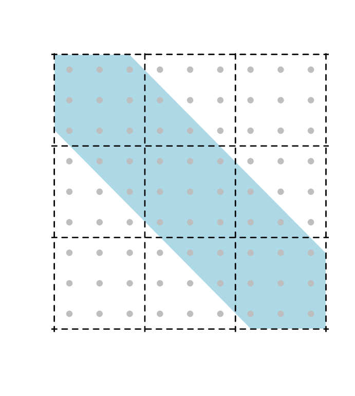
Figure 1: An illustration of block partition for the banding estimator with $p=9$ and $K=3$. Each filled circle is an entry and these entries outside the shaded area are truncated to 0. The off-diagonal blocks have only $K*(K-1)/2=3$ non-zero entries.

Now we know each row or column of $(\hat{\Sigma}_{K}-\Sigma_{K})^{\ast}$ has at most three non-zero entries. By the norm compression inequality in [9],

$$\|\hat{\Sigma}_{K}-\Sigma_{K}\|_{op}\leq\|(\hat{\Sigma}_{K}-\Sigma_{K})^{\ast}\|_{op}\leq 3\max_{|k-\ell|\leq 1}\|\hat{\Sigma}_{K}(k,\ell)-\Sigma_{K}(k,\ell)\|_{op},$$

where the second inequality follows by (2.1). Then Proposition 1 is proved by Proposition 2. ∎

Proposition 2.

There exists a constant $c>0$ such that

$$\mathbb{P}\left\{\max_{|k-\ell|\leq 1}\|\hat{\Sigma}_{K}(k,\ell)-\Sigma_{K}(k,\ell)\|_{op}\geq c\|\Sigma^{abs}\|_{op}\sqrt{\frac{K+\log p}{n}}\right\}\lesssim p^{-1}.$$

Furthermore,

$$\mathbb{E}\max_{|k-\ell|\leq 1}\|\hat{\Sigma}_{K}(k,\ell)-\Sigma_{K}(k,\ell)\|_{op}^{2}\lesssim\frac{K+\log p}{n}.$$

Remark 2.

The proposition provides probability and risk bounds for sample covariance matrix and for sample cross covariance matrix with upper triangular elements fixed at zero, and hence extends results in [6], which considers only sample covariance matrix, and also complements Lemma 2 in [9], which considers sample cross covariance matrices.

Remark 3.

The probability bound on $\|\hat{\Sigma}_{K}(k,\ell)-\Sigma_{K}(k,\ell)\|_{op}$ for $k-\ell=\pm 1$ is non-standard, as the matrices involved have irregular forms and fixed zero entries. The derivation of this bound requires concentration inequalities for the bilinear form $X^{T}AY$ where $X$ and $Y$ are multivariate random vectors and $A$ is an arbitrary non-random matrix. To our best knowledge, such concentration inequalities have not been derived in the literature, in which only the special case $X=Y$ and $A$ is symmetric have been treated, see e.g. [5]. We provide these inequalities in Proposition 4 in the appendix.

The proof of Proposition 2 is deferred to Section 5.

3 Sure-tuned Bandwidth Selection

This section is devoted to the selection of the bandwidth of an operator-norm accurate estimator. One possibility, as in [3], is to use cross validation. If operator norm is used for defining the loss function, cross validation can be computationally quite intensive for large $p$ because about $O(p)$ operator norms of $p\times p$ matrices have to be evaluated. [3] used the maximum row sum norm $\|\cdot\|_{1,1}$ for defining the loss function. We propose an alternative approach, with low computational complexity. Our procedure minimizes in $K$ a data-driven criterion that is a function of the bandwidth $K$. The proposed criterion is a modified unbiased estimator of the Frobenius-norm risk of $\hat{\Sigma}_{K}$, and its derivation follows the general principles of Stein’s unbiased risk estimation (Sure) [26].

To begin, note that the Frobenius risk of $\hat{\Sigma}_{K}$ is

$$\mathbb{E}\|\hat{\Sigma}_{K}-\Sigma\|_{F}^{2} =\sum_{|i-j|\leq K-1}\mathbb{E}(\hat{\sigma}_{ij}-\sigma_{ij})^{2}+\sum_{|i-j|\geq K}\sigma_{ij}^{2}$$

$$=\sum_{|i-j|\leq K-1}\text{Var}(\hat{\sigma}_{ij})+\sum_{|i-j|\geq K}\sigma_{ij}^{2}.$$

The first term above is the sum of variances of the entries in $\hat{\Sigma}_{K}$ while the second term is the sum of squared biases of $\hat{\Sigma}_{K}$. The following proposition provides unbiased estimates of $\text{Var}(\hat{\sigma}_{ij})$ and $\sigma_{ij}^{2}$.

Proposition 3.

$$\text{Var}(\hat{\sigma}_{ij})=\frac{\sigma_{ii}\sigma_{jj}+\sigma_{ij}^{2}}{n-1}$$ (3.1)

and an unbiased estimate of $\text{Var}(\hat{\sigma}_{ij})$ can be given by

$$\widehat{\text{Var}}(\hat{\sigma}_{ij})=a_{n}\hat{\sigma}_{ii}\hat{\sigma}_{jj}+b_{n}\hat{\sigma}_{ij}^{2},$$

where $a_{n}=\frac{n-1}{n^{2}-n-2}$ and $b_{n}=\frac{n-3}{n^{2}-n-2}$. Moreover, an unbiased estimate of $\sigma_{ij}^{2}$ can be given by $c_{n}\hat{\sigma}_{ii}\hat{\sigma}_{jj}+d_{n}\hat{\sigma}_{ij}^{2},$ where $c_{n}=\frac{1-n}{n^{2}-n-2}$ and $d_{n}=\frac{(n-1)^{2}}{n^{2}-n-2}$.

Remark 4.

The proof is omitted as it follows straightforwardly from Lemma 1 in the appendix. Equation (3.1) was first derived by [29].

By Proposition 3, an unbiased estimate of the Frobenius risk of $\hat{\Sigma}_{K}$ can therefore be given by:

$$\mbox{Sure}_{F}(K)=\sum_{|i-j|\leq K-1}\left(a_{n}\hat{\sigma}_{ii}\hat{\sigma}_{jj}+b_{n}\hat{\sigma}_{ij}^{2}\right)+\sum_{|i-j|\geq K}\left(c_{n}\hat{\sigma}_{ii}\hat{\sigma}_{jj}+d_{n}\hat{\sigma}_{ij}^{2}\right).$$ (3.2)

One could then select

$$\hat{K}_{F}=\arg\min_{K}\text{Sure}_{F}(K).$$

A similar procedure has been suggested in [29], but for tapering estimators.

We denote by $\hat{P}_{F}$ the Sure-tuned banding estimator with bandwidth equal to $\hat{K}_{F}$. The estimator $\hat{P}_{F}$ is appropriate if the goal is to construct a Frobenius-norm accurate estimator. However, it is known from the theoretic analysis in [10] that the bandwidth for optimal Frobenius norm estimation is asymptotically smaller than what is needed for optimal operator norm estimation. We propose some modification to criterion (3.2) above, that will encourage the selection of a larger bandwidth. The idea is to place a larger weight on the bias term, which is the second sum in (3.2), so that a larger bandwidth is selected. We do this via the factor $K$ in the weights $W_{ijK}$ given by (3.3) below. Moreover, we notice that, over the class $\mathcal{C}_{\alpha}$, the entries $\sigma_{ij}^{2}$ corresponding to large $|i-j|$ are small, but their estimates $c_{n}\hat{\sigma}_{ii}\hat{\sigma}_{jj}+d_{n}\hat{\sigma}_{ij}^{2}$, albeit unbiased, have variability that can be much higher than the size of $\sigma_{ij}^{2}$. Therefore, for a more stable selection of $K$, we attenuate the contribution of the estimates of $\sigma_{ij}^{2}$ with large $|i-j|$ via the exponentially decaying factor in (3.3).

Therefore we use the following criterion

$$\text{Sure}_{op}(K)=\sum_{|i-j|\leq K-1}\left(a_{n}\hat{\sigma}_{ii}\hat{\sigma}_{jj}+b_{n}\hat{\sigma}_{ij}^{2}\right)+\sum_{|i-j|\geq K}W_{ijK}\left(c_{n}\hat{\sigma}_{ii}\hat{\sigma}_{jj}+d_{n}\hat{\sigma}_{ij}^{2}\right),$$

where

$$W_{ijK}=K\exp\left(1-\frac{|i-j|}{K}\right),$$ (3.3)

and select

$$\hat{K}_{op}=\arg\min_{K}\text{Sure}_{op}(K).$$

We call the banding estimator with bandwidth $\hat{K}_{op}$ the “modified Sure-tuned banding estimator” and denote it by $\hat{P}_{op}$. We now give a heuristic argument why the above approach might select a bandwidth that is well-suited for estimation under the operator norm. We assume $|\sigma_{ij}|\leq M_{1}|i-j|^{-\alpha-1}$ for all $(i,j)$. Then

$$\mathbb{E}\text{Sure}_{op}(K) =\sum_{|i-j|\leq K-1}\text{Var}(\hat{\sigma}_{ij})+\sum_{|i-j|\geq K}KW_{ijK}\sigma_{ij}^{2}$$

$$=O(K/n)+O\left\{\sum_{|i-j|\geq K}\exp\left(1-\frac{|i-j|}{K}\right)K^{-(2\alpha+1)}\right\}$$

$$=O(K/n)+O(K^{-2\alpha}).$$

Hence $\mathbb{E}\text{Sure}_{op}(K)$ is minimized only if $K=O\left(n^{-\frac{1}{2\alpha+1}}\right)$, and we recall that in Remark 1 above we showed that the optimal bandwidth for operator-norm estimation is of this order. We further demonstrate experimentally in the following section that the estimator with a bandwidth thus selected has excellent operator norm behavior.

4 Simulations

We compare the following 6 estimators:

1. $\hat{P}_{cv}$: the banding estimator for which the bandwidth is selected by 10-fold cross validation with squared operator norm as the loss function ;

2. $\hat{P}_{BL}$: the banding estimator in [3] for which the bandwidth is selected by 10-fold cross validation with the maximum row sum norm $\|\cdot\|_{1,1}$ as the loss function;

3. $\hat{P}_{CY}$: the block-thresholding estimator in [9];

4. $\hat{P}_{YZ}$: the Sure-tuned tapering estimator in [29];

5. $\hat{P}_{F}$: the Sure-tuned banding estimator;

6. $\hat{P}_{op}$: the modified Sure-tuned banding estimator.

The data are generated from $\mathcal{N}(0,\Sigma$). Following [3] and [10], the covariance matrix $\Sigma$ has the following form

$$\sigma_{ij}=\rho|i-j|^{-(\alpha+1)},$$

where $\rho=0.6$ and $\alpha$ can be either $0.1$ or $0.5$. Similar to [29], we fix $n$ at 250 and let $p$ be either of 250, 500 and 1000. For each scenario, we run 100 simulations and compute the mean squared errors in terms of the operator norm. For example, for the re-weighted Sure-tuned banding estimator $\hat{P}_{op}$, its mean squared error is

$$\frac{1}{100}\sum_{k=1}^{100}\|\hat{P}_{op}^{k}-\Sigma\|_{op}^{2},$$

where $\hat{P}_{op}^{k}$ is the estimate for the $k$th simulated dataset. It is noted by [29] that the optimal bandwidth for the operator norm can be quite variable. To reduce the variability of the selected bandwidth, $\hat{K}_{op}$ will be restricted to the interval $[\hat{K}_{F},\hat{K}_{F}^{2}]$.

Table 1 gives the simulation results. Several observations can be made from Table 1. First, the estimator $\hat{P}_{cv}$ using cross-validation, one of the most widely used statistical techniques, has the worst performance in this problem. We note that calculation of $\hat{P}_{cv}$ is also very time consuming when $p$ is large. Secondly, it is interesting to see that the operator-norm rate-optimal $\hat{P}_{CY}$ is dominated by three other Sure-type estimators, $\hat{P}_{FZ}$, $\hat{P}_{F}$ and $\hat{P}_{op}$. Third, the Sure-tuned banding and tapering estimators, $\hat{P}_{FZ}$ and $\hat{P}_{F}$, have comparable MSEs and the modified Sure-tuned banding estimator $\hat{P}_{op}$ always has the smallest MSEs, except for one scenario. The modified Sure-tuned banding estimator $\hat{P}_{op}$ has larger standard error than $\hat{P}_{FZ}$ and $\hat{P}_{F}$ because of the larger variability of the selected bandwidth (results not shown).

Table 1: Mean and standard deviations (in parenthesis) of squared errors in operator norm for the 6 estimators.

$\alpha$	$p$	$\hat{P}_{cv}$	$\hat{P}_{BL}$	$\hat{P}_{CY}$	$\hat{P}_{YZ}$	$\hat{P}_{F}$	$\hat{P}_{op}$
$0.1$	250	7.96 (4.59)	6.07 (3.27)	13.34 (0.26)	5.36 (0.67)	5.38 (0.64)	4.61 (1.37)
	500	17.68 (12.32)	8.36 (5.01)	15.86 (0.24)	7.73 (0.69)	7.85 (0.65)	6.05 (1.51)
	1,000	37.20 (28.78)	10.88 (7.21)	19.81 (0.18)	10.59 (0.60)	10.56 (0.49)	8.16 (1.78)
$0.5$	250	6.08 (4.60)	3.48 (3.23)	2.72 (0.12)	1.08 (0.13)	1.07 (0.14)	1.13 (0.32)
	500	12.59 (11.01)	4.44 (5.88)	2.62 (0.09)	1.22 (0.08)	1.21 (0.10)	1.18 (0.23)
	1,000	31.88 (32.18)	6.51(14.10)	2.79 (0.07)	1.35 (0.07)	1.33 (0.07)	1.27 (0.32)

5 Proof of Proposition 2

Proof.

We start with studying $u^{T}\left\{\hat{\Sigma}(k,\ell)*H-\Sigma(k,\ell)*H\right\}v$, where $u,v\in\mathbb{S}^{K-1}$. Assume $X$ and $Y$ have a joint real normal distribution $\textnormal{MVN}_{2K}(0,\Sigma^{1})$ with

$$\Sigma^{1}=\left(\begin{array}[]{cc}\Sigma_{11}&\Sigma_{12}\\ \Sigma_{21}&\Sigma_{22}\end{array}\right)$$

and

$$\Sigma_{11}=\Sigma(k,k),\Sigma_{22}=\Sigma(\ell,\ell),\Sigma_{12}=\Sigma_{21}^{T}=\Sigma(k,\ell).$$

Let $A=(uv^{T})*H$. Then $u^{T}\left\{\hat{\Sigma}(k,\ell)*H-\Sigma(k,\ell)*H\right\}v$ is the same in distribution as

$$\frac{1}{n-1}\sum_{i=1}^{n}(X_{i}-\bar{X})^{T}A(Y_{i}-\bar{Y})-{\textrm{t}r}(A\Sigma_{21}),$$

where $(X_{1},Y_{1}),\dots,(X_{n},Y_{n})$ are i.i.d. copies of $(X,Y)$, $\bar{X}=n^{-1}\sum_{i=1}^{n}X_{i}$, and $\bar{Y}=n^{-1}\sum_{i=1}^{n}Y_{i}$. It is easy to show that $\mathbb{E}(X_{i}^{T}AY_{i})={\textrm{t}r}(A\Sigma_{21})$ and $\mathbb{E}(\bar{X}^{T}A\bar{Y})=n^{-1}{\textrm{t}r}(A\Sigma_{21})$. Therefore,

$$\begin{split}&\frac{1}{n-1}\sum_{i=1}^{n}(X_{i}-\bar{X})^{T}A(Y_{i}-\bar{Y})-{\textrm{t}r}(A\Sigma_{21})\\ =&\frac{n}{n-1}\left[\frac{1}{n}\sum_{i=1}^{n}\left\{X_{i}^{T}AY_{i}-\mathbb{E}(X_{i}^{T}AY_{i})\right\}-\left\{\bar{X}^{T}A\bar{Y}-\mathbb{E}(\bar{X}^{T}A\bar{Y})\right\}\right].\end{split}$$ (5.1)

We first consider the term $n^{-1}\sum_{i=1}^{n}\left\{X_{i}^{T}AY_{i}-\mathbb{E}(X_{i}^{T}AY_{i})\right\}$ in (5.1). Let $Q_{i}=X_{i}^{T}AY_{i},i=1,\dots,n$, then $Q_{1},\dots,Q_{n}$ are i.i.d. copies of $Q=X^{T}AY$. Let $\bar{Q}=n^{-1}\sum_{i=1}^{n}(Q_{i}-\mathbb{E}Q_{i})$, which equals $n^{-1}\sum_{i=1}^{n}\left\{X_{i}^{T}AY_{i}-\mathbb{E}(X_{i}^{T}AY_{i})\right\}$ in distribution. By Proposition 4, for $0<t<1/2$,

$$\mathbb{P}\left\{|\bar{Q}|>t\sqrt{{\textrm{t}r}(B^{2})}\right\}\leq 2\exp\left(-\frac{nt^{2}}{2}\right),$$

where

$$B=\Sigma^{1,1/2}\left(\begin{array}[]{cc}0_{K,K}&A\\ A^{T}&0_{K,K}\end{array}\right)\Sigma^{1,1/2}.$$

By Lemma 5 we have

$${\textrm{t}r}(B^{2})\leq 4\|\Sigma^{1,abs}\|_{op}^{2}\leq 4\|\Sigma^{abs}\|_{op}^{2}$$

Therefore,

$$\mathbb{P}\left\{|\bar{Q}|>2t\|\Sigma^{abs}\|_{op}\right\}\leq 2\exp\left(-\frac{nt^{2}}{2}\right),$$

or equivalently,

$$\mathbb{P}\left\{\left|\frac{1}{n}\sum_{i=1}^{n}\left\{X_{i}^{T}AY_{i}-\mathbb{E}(X_{i}^{T}AY_{i})\right\}\right|>2t\|\Sigma^{abs}\|_{op}\right\}\leq 2\exp\left(-\frac{nt^{2}}{2}\right).$$ (5.2)

We next consider the term $\bar{X}^{T}A\bar{Y}-\mathbb{E}(\bar{X}^{T}A\bar{Y})$ in (5.1). Note that $\bar{X}$ and $\bar{Y}$ have a joint real normal distribution $\text{MVN}(0,n^{-1}\Sigma^{1})$. By similar derivation as above,

$$\mathbb{P}\left\{\left|\bar{X}^{T}A\bar{Y}-\mathbb{E}(\bar{X}^{T}A\bar{Y})\right|>2t\|\Sigma^{abs}\|_{op}/n\right\}\leq 2\exp\left(-\frac{t^{2}}{2}\right),$$

or equivalently,

$$\mathbb{P}\left\{\left|\bar{X}^{T}A\bar{Y}-\mathbb{E}(\bar{X}^{T}A\bar{Y})\right|>2t\|\Sigma^{abs}\|_{op}\right\}\leq 2\exp\left(-\frac{n^{2}t^{2}}{2}\right).$$ (5.3)

Note that for any two random variables $Z_{1}$ and $Z_{2}$,

$$\mathbb{P}(|Z_{1}-Z_{1}|>2x)\leq\mathbb{P}(|Z_{1}|>x)+\mathbb{P}(|Z_{2}|>x).$$

Combining (5.1), (5.2) and (5.3), we obtain

$$\mathbb{P}\left[\left|u^{T}\left\{\hat{\Sigma}(k,\ell)*H-\Sigma(k,\ell)*H\right\}v\right|>\frac{4(n-1)}{n}\|\Sigma^{abs}\|_{op}t\right]$$

$$\leq 2\exp\left(-\frac{nt^{2}}{2}\right)+2\exp\left(-\frac{n^{2}t^{2}}{2}\right),$$

which leads to

$$\mathbb{P}\left[\left|u^{T}\left\{\hat{\Sigma}(k,\ell)*H-\Sigma(k,\ell)*H\right\}v\right|>4\|\Sigma^{abs}\|_{op}t\right]\leq 4\exp\left(-\frac{nt^{2}}{2}\right).$$ (5.4)

Now we consider $\|\hat{\Sigma}(k,\ell)*H-\Sigma(k,\ell)*H\|_{op}$. By Lemma 6, there exists an $\delta$-net $\mathbb{Q}_{K}\in\mathbb{S}^{K-1}$ such that

$$\text{card}(\mathbb{Q}_{K})\leq c_{1}\delta^{-K}K^{3/2}\log(1+K)$$

for some constant $c_{1}>0$. It can also be shown that

$$\|\hat{\Sigma}(k,\ell)*H-\Sigma(k,\ell)*H\|_{op}$$

$$= \sup_{u,v\in\mathbb{S}^{K-1}}u^{T}\left\{\hat{\Sigma}(k,\ell)*H-\Sigma(k,\ell)*H\right\}v.$$

$$\geq (1-2\delta)^{-1}\sup_{u,v\in\mathbb{Q}^{K-1}}u^{T}\left\{\hat{\Sigma}(k,\ell)*H-\Sigma(k,\ell)*H\right\}v.$$

By (5.4) and the union bound,

$$\mathbb{P}\left[\max_{|k-\ell|\leq 1}\|\hat{\Sigma}(k,\ell)*H-\Sigma(k,\ell)*H\|_{op}>t\right]$$

$$\leq \mathbb{P}\left[\max_{|k-\ell|\leq 1}\sup_{u,v\in\mathbb{Q}_{K}}u^{T}\left\{\hat{\Sigma}(k,\ell)*H-\Sigma(k,\ell)*H\right\}v>(1-2\delta)t\right]$$

$$\leq 12c_{1}p\delta^{-2K}K^{3}\log^{2}(1+K)\exp\left\{-\frac{nt^{2}(1-2\delta)^{2}}{32\|\Sigma^{abs}\|_{op}^{2}}\right\}.$$

To summarize, if we let $W=\max_{|k-\ell|\leq 1}\|\hat{\Sigma}(k,\ell)*H-\Sigma(k,\ell)*H\|_{op}$, then

$$\mathbb{P}(W>t)\leq 12cp\delta^{-2K}K^{3}\log^{2}(1+K)\exp\left\{-\frac{nt^{2}(1-2\delta)^{2}}{32\|\Sigma^{abs}\|_{op}^{2}}\right\}.$$ (5.5)

To establish the probability bound in Proposition 2, similar to [9] we just need to rewrite (5.5) by letting $\delta=\exp(-3)$, $c_{0}=\sqrt{192}/(1-2\delta)$ and

$$t=c_{0}\|\Sigma^{abs}\|_{op}\sqrt{\frac{K+\log p}{n}}.$$

The inequality in expectation can be similarly derived by (5.5) and the fact that

$$\mathbb{E}W^{2}\leq x+\int_{x}^{\infty}\mathbb{P}(W^{2}>t)dt$$

for any $x>0$. ∎

Appendix A A Lemma for Proposition 3

Lemma 1.

$$\mathbb{E}(\hat{\sigma}_{ij}^{2}) = \frac{1}{n-1}\sigma_{ii}\sigma_{jj}+\frac{n}{n-1}\sigma_{ij}^{2},$$ (A.1)

$$\mathbb{E}(\hat{\sigma}_{ii}\hat{\sigma}_{jj}) = \sigma_{ii}\sigma_{jj}+\frac{2}{n-1}\sigma_{ij}^{2}.$$ (A.2)

Remark 5.

[29] derived the above equalities, however, their result on $\mathbb{E}(\hat{\sigma}_{ii}\hat{\sigma}_{jj})$ is incorrect; see equations (A.7) and (A.12) therein. A quick check is to let $i=j$.

Proof.

We assume w.l.o.g. that $\mu=0$. We use $\bar{x}_{i}$ to denote $n^{-1}\sum_{k=1}^{n}x_{k,i}$. Note that he following equation for all pairs of $(i,j)$,

$$\mathbb{E}(x_{i}^{2}x_{j}^{2})=\sigma_{ii}\sigma_{jj}+2\sigma_{ij}^{2}.$$ (A.3)

It’s straightforward to show that

$$(n-1)\hat{\sigma}_{ij}=\sum_{k=1}^{n}x_{k,i}x_{k,j}-n\bar{x}_{i}\bar{x}_{j}.$$

Note that

$$(\bar{x}_{i},\bar{x}_{j},x_{1,i},x_{1,j})^{T}\sim\text{MVN}\left(0,\left(\begin{array}[]{cccc}\frac{\sigma_{ii}}{n}&\frac{\sigma_{ij}}{n}&\frac{\sigma_{ii}}{n}&\frac{\sigma_{ij}}{n}\\ \frac{\sigma_{ij}}{n}&\frac{\sigma_{jj}}{n}&\frac{\sigma_{ij}}{n}&\frac{\sigma_{ij}}{n}\\ \frac{\sigma_{ii}}{n}&\frac{\sigma_{ij}}{n}&\sigma_{ii}&\sigma_{ij}\\ \frac{\sigma_{ij}}{n}&\frac{\sigma_{ij}}{n}&\sigma_{ij}&\sigma_{jj}\end{array}\right)\right).$$

Hence

$$\mathbb{E}(\bar{x}_{i}^{2}x_{1,j}^{2}) = \sigma_{ii}\sigma_{jj}/n+2\sigma_{ij}^{2}/n,$$ (A.4)

$$\mathbb{E}(\bar{x}_{i}^{2}\bar{x}_{j}^{2}) = \sigma_{ii}\sigma_{jj}/n^{2}+2\sigma_{ij}^{2}/n^{2},$$ (A.5)

$$\mathbb{E}(\bar{x}_{i}\bar{x}_{j}x_{1,i}x_{1,j}) = \sigma_{ii}\sigma_{jj}/n^{2}+\sigma_{ij}^{2}(1/n+1/n^{2}).$$ (A.6)

We first derive (A.1) by using (A.3), (A.5) and (A.6). We have

$$(n-1)^{2}\mathbb{E}(\hat{\sigma}_{ij}^{2})$$

$$=\mathbb{E}\left(\sum_{k=1}^{n}x_{k,i}x_{k,j}-n\bar{x}_{i}\bar{x}_{j}\right)^{2}$$

$$=\mathbb{E}\left(\sum_{k=1}^{n}x_{k,i}x_{k,j}\right)^{2}-2n\mathbb{E}\left(\bar{x}_{i}\bar{x}_{j}\sum_{k=1}^{n}x_{k,i}x_{k,j}\right)+n^{2}\mathbb{E}(\bar{x}_{i}^{2}\bar{x}_{j}^{2})$$

$$=\sum_{k,k^{\prime}}\mathbb{E}(x_{k,i}x_{k,j}x_{k^{\prime},i}x_{k^{\prime},j})-2n^{2}\mathbb{E}(\bar{x}_{i}\bar{x}_{j}x_{1,i}x_{1,j})+n^{2}\mathbb{E}(\bar{x}_{i}^{2}\bar{x}_{j}^{2})$$

$$=\sum_{k=k^{\prime}}(\sigma_{ii}\sigma_{jj}+2\sigma_{ij}^{2})+\sum_{k\neq k^{\prime}}\sigma_{ij}^{2}-2(\sigma_{ii}\sigma_{jj}+(n+1)\sigma_{ij}^{2})+(\sigma_{ii}\sigma_{jj}+2\sigma_{ij}^{2})$$

$$=(n-1)\sigma_{ii}\sigma_{jj}+n(n-1)\sigma_{ij}^{2},$$

which proves (A.1).

Next we derive (A.2) by using (A.3), (A.4) and (A.5). We have

$$(n-1)^{2}\mathbb{E}(\hat{\sigma}_{ii}\hat{\sigma}_{jj})$$

$$=\mathbb{E}\left\{\left(\sum_{k=1}^{n}x_{k,i}^{2}-n\bar{x}_{i}^{2}\right)\left(\sum_{k=1}^{n}x_{k,j}^{2}-n\bar{x}_{j}^{2}\right)\right\}$$

$$=\sum_{k,k^{\prime}}\mathbb{E}(x_{k,i}^{2}x_{k^{\prime},j}^{2})-n\sum_{k}\mathbb{E}(\bar{x}_{i}^{2}x_{k,j}^{2})-n\sum_{k}\mathbb{E}(\bar{x}_{j}^{2}x_{k,i}^{2})+n^{2}\mathbb{E}(\bar{x}_{i}^{2}\bar{x}_{j}^{2})$$

$$=\sum_{k=k^{\prime}}(\sigma_{ii}\sigma_{jj}+2\sigma_{ij}^{2})+\sum_{k\neq k^{\prime}}(\sigma_{ii}\sigma_{jj})-n^{2}\mathbb{E}(\bar{x}_{i}^{2}x_{1,j}^{2})-n^{2}\mathbb{E}(\bar{x}_{j}^{2}x_{1,i}^{2})+n^{2}\mathbb{E}(\bar{x}_{i}^{2}\bar{x}_{j}^{2})$$

$$=n^{2}\sigma_{ii}\sigma_{jj}+2n\sigma_{ij}^{2}-2(n\sigma_{ii}\sigma_{jj}+2\sigma_{ij}^{2})+(\sigma_{ii}\sigma_{jj}+2\sigma_{ij}^{2})$$

$$=(n-1)^{2}\sigma_{ii}\sigma_{jj}+2(n-1)\sigma_{ij}^{2},$$

which proves (A.2).

∎

Appendix B Supplemental materials for Section 5

Proposition 4.

Let the $p\times 1$ vector $X$ and $q\times 1$ vector $Y$ have a joint real normal distribution $\text{MVN}_{p+q}(0,\Sigma),\Sigma>0$. Let $A$ be a $p\times q$ real matrix. Let $Q=X^{T}AY$. Let $Q_{1},\dots,Q_{n}$ be i.i.d. realizations of $Q$. Denote $\bar{Q}=n^{-1}\sum_{i=1}^{n}(Q_{i}-\mathbb{E}Q_{i})$. Then, for $0<t<1/2$,

$$\mathbb{P}\left\{|\bar{Q}|>t\sqrt{{\textrm{t}r}(B^{2})}\right\}\leq 2\exp\left(-\frac{nt^{2}}{2}\right),$$

where

$$B=\Sigma^{1/2}\left(\begin{array}[]{cc}0_{K,K}&A\\ A^{T}&0_{K,K}\end{array}\right)\Sigma^{1/2}.$$

Remark 6.

The proposition also follows if $X=Y$ by the remark right after Lemma 3.

Proof.

By Lemma 3,

$$\mathbb{E}\exp\left\{t(Q-\mathbb{E}Q)\right\}\leq\exp\left\{\frac{1}{2}t^{2}{\textrm{t}r}(B^{2})\right\}$$

for $|t|<\frac{1}{2\|B\|_{op}}$. Then

$$\mathbb{E}\exp(t\bar{Q})\leq\exp\left\{\frac{{\textrm{t}r}(B^{2})}{2n}t^{2}\right\}$$

for $|t|<\frac{n}{2\|B\|_{op}}$. An application of Lemma 4 yields

$$\mathbb{P}\left\{|\bar{Q}|>t\sqrt{{\textrm{t}r}(B^{2})}\right\}\leq 2\exp\left(-\frac{nt^{2}}{2}\right)$$

for $0<t<\frac{\sqrt{{\textrm{t}r}(B^{2})}}{2\|B\|_{op}}$. It is easy to show that $\sqrt{{\textrm{t}r}(B^{2})}/\|B\|_{op}\geq 1$, hence we can always let $0<t<1/2$.

∎

Lemma 2.

For $x>-1/2$,

$$\log(1+x)-x+x^{2}\geq 0.$$

Proof.

Let $f(x)=\log(1+x)-x+x^{2}$. Then

$$\frac{\partial f(x)}{\partial x}=\frac{1}{1+x}-1+2x=\frac{x(2x+1)}{x+1}.$$

So $\frac{\partial f(x)}{\partial x}<0$ if $-1/2<x<0$, $\frac{\partial f(x)}{\partial x}>0$ if $x>0$, and $f(0)=0$, which leads to $f(x)\geq 0$ for all $x>-1/2$. ∎

Lemma 3.

Let the $p\times 1$ vector $X$ and $q\times 1$ vector $Y$ have a joint real normal distribution $\textnormal{MVN}_{p+q}(0,\Sigma)$, $\Sigma>0$. Let $A$ be a $p\times q$ real matrix. Let $Q=X^{T}AY$. Then

$$\mathbb{E}\exp(tQ)=\frac{1}{\sqrt{\textnormal{det}\left(I_{p+q,p+q}-tB\right)}}$$ (B.1)

for $|t|<\frac{1}{2\|B\|_{op}}$, where $\textnormal{det}(\cdot)$ denotes the determinant of a square matrix and

$$B=\Sigma^{1/2}\left(\begin{array}[]{cc}0_{p,p}&A\\ A^{T}&0_{q,q}\end{array}\right)\Sigma^{1/2}.$$

Moreover,

$$\mathbb{E}\exp\left\{t(Q-\mathbb{E}Q)\right\}\leq\exp\left\{\frac{1}{2}t^{2}{\textrm{t}r}(B^{2})\right\}$$ (B.2)

for $|t|<\frac{1}{2\|B\|_{op}}$, where $\mathbb{E}Q={\textrm{t}r}(B)/2$.

Remark 7.

If $X=Y$, inequality (B.2) still holds.

Proof.

[22] showed that

$$\mathbb{E}\exp(tQ)=\frac{1}{\sqrt{\textnormal{det}\left\{\Sigma^{-1}-t\left(\begin{array}[]{cc}0_{p,p}&A\\ A^{T}&0_{q,q}\end{array}\right)\right\}\textnormal{det}(\Sigma)}}$$

which leads to equation (B.1) by using the equality $\textnormal{det}(UV)=\textnormal{det}(U)\textnormal{det}(V)$ for square matrices $U$ and $V$ and that $\textnormal{det}(\Sigma)=\textnormal{det}(\Sigma^{1/2})\textnormal{det}(\Sigma^{1/2})$. Let $\{\lambda_{1},\dots,\lambda_{p+q}\}$ denote the collection of all eigenvalues of $B$. Then

$$\mathbb{E}\exp(tQ) =\prod_{k=1}^{p+q}(1-t\lambda_{k})^{-1/2}$$

$$=\exp\left\{-\frac{1}{2}\sum_{k=1}^{p+q}\log(1-t\lambda_{k})\right\}$$

$$\leq\exp\left\{-\frac{1}{2}\sum_{k=1}^{p+q}(-t\lambda_{k}-t^{2}\lambda_{k}^{2})\right\}$$

$$=\exp\left\{\frac{1}{2}t\sum_{k=1}^{p+q}\lambda_{k}+\frac{1}{2}t^{2}\sum_{k=1}^{p+q}\lambda_{k}^{2}\right\}.$$

In the above inequality we applied Lemma 2 for each $\log(1-t\lambda_{k})$. Note that

$$\sum_{k=1}^{p+q}\lambda_{k} ={\textrm{t}r}(B)$$

$$={\textrm{t}r}\left\{\left(\begin{array}[]{cc}0_{p,p}&A\\ A^{T}&0_{q,q}\end{array}\right)\Sigma\right\}$$

$$={\textrm{t}r}\left\{\left(\begin{array}[]{cc}0_{p,p}&A\\ A^{T}&0_{q,q}\end{array}\right)\left(\begin{array}[]{cc}\Sigma_{11}&\Sigma_{12}\\ \Sigma_{21}&\Sigma_{22}\end{array}\right)\right\}$$

$$=2{\textrm{t}r}(A\Sigma_{21})$$

$$=2\mathbb{E}Q$$

and

$$\sum_{k=1}^{p+q}\lambda_{k}^{2}={\textrm{t}r}(B^{2}).$$

Hence

$$\mathbb{E}\exp\left\{t(Q-\mathbb{E}Q)\right\}\leq\exp\left\{\frac{1}{2}t^{2}{\textrm{t}r}(B^{2})\right\}$$

which is (B.2). ∎

Lemma 4.

Let $c_{0}$ and $c_{1}$ be two constants greater than 0. Let $Q$ be a real random variable with mean zero and satisfies

$$\mathbb{E}\exp(tQ)\leq\exp(c_{0}t^{2})$$

for any $|t|<c_{1}$. Then for $0<t<2c_{0}c_{1}$,

$$\mathbb{P}\left\{Q\geq t\right\}\leq\exp\left(-\frac{t^{2}}{4c_{0}}\right)$$

and

$$\mathbb{P}\left\{Q\leq-t\right\}\leq\exp\left(-\frac{t^{2}}{4c_{0}}\right).$$

Proof.

Let $a=t/(2c_{0})$. Then

$$\mathbb{P}(Q>t) =\mathbb{P}\left\{\exp(aQ)>\exp(at)\right\}$$

$$\leq\exp(-at)\mathbb{E}\exp(aQ)$$

$$\leq\exp(c_{0}a^{2}-at)$$

$$=\exp\left(-\frac{t^{2}}{4c_{0}}\right)$$

Similarly we derive that

$$\mathbb{P}(Q<-t)\leq\exp\left(-\frac{t^{2}}{4c_{0}}\right)$$

and the proof is complete. ∎

Lemma 5.

Let $A=(uv^{T})*H$, where $u,v\in\mathbb{S}^{K-1}$ and $H=(h_{k\ell})_{1\leq k,\ell\leq K}$ with $|h_{k\ell}|\leq 1$ for all $(k,\ell)$. Let $\Sigma$ be an $2K\times 2K$ covariance matrix with 4 $K\times K$ blocks

$$\Sigma=\left(\begin{array}[]{cc}\Sigma_{11}&\Sigma_{12}\\ \Sigma_{21}&\Sigma_{22}\end{array}\right).$$

Let

$$B=\Sigma^{1/2}\left(\begin{array}[]{cc}0_{K,K}&A\\ A^{T}&0_{K,K}\end{array}\right)\Sigma^{1/2}.$$

Then

$${\textrm{t}r}(B^{2})\leq 2\|\Sigma_{12}^{abs}\|_{op}^{2}+2\|\Sigma_{11}^{abs}\|_{op}\|\Sigma_{22}^{abs}\|_{op},$$

where for a matrix $C=(c_{k\ell})_{1\leq k,\ell\leq K}$, $C^{abs}=(|c_{k\ell}|)_{1\leq k,\ell\leq K}$.

Proof.

First we have ${\textrm{t}r}(B^{2})={\textrm{t}r}(C^{2}),$ where

$$C= \left(\begin{array}[]{cc}0_{K,K}&A\\ A^{T}&0_{K,K}\end{array}\right)\Sigma$$

$$= \left(\begin{array}[]{cc}A\Sigma_{21}&A\Sigma_{22}\\ A^{T}\Sigma_{11}&A^{T}\Sigma_{12}\end{array}\right).$$

Next

$${\textrm{t}r}(C^{2})= {\textrm{t}r}(A\Sigma_{21}A\Sigma_{21}+A\Sigma_{22}A^{T}\Sigma_{11}+A^{T}\Sigma_{11}A\Sigma_{22}+A^{T}\Sigma_{12}A^{T}\Sigma_{12})$$

$$= 2{\textrm{t}r}(A^{T}\Sigma_{12}A^{T}\Sigma_{12})+2{\textrm{t}r}(A^{T}\Sigma_{11}A\Sigma_{22})$$

$$\leq 2{\textrm{t}r}(A^{abs,T}\Sigma_{12}^{abs}A^{abs,T}\Sigma_{12}^{abs})+2{\textrm{t}r}(A^{abs,T}\Sigma_{11}^{abs}A^{abs}\Sigma_{22}^{abs})$$

$$\leq 2{\textrm{t}r}(v^{abs}u^{abs,T}\Sigma_{12}^{abs}v^{abs}u^{abs,T}\Sigma_{12}^{abs})+2{\textrm{t}r}(v^{abs}u^{abs,T}\Sigma_{11}^{abs}u^{abs}v^{abs,T}\Sigma_{22}^{abs})$$

$$= 2(u^{abs,T}\Sigma_{12}v^{abs})^{2}+2(u^{abs,T}\Sigma_{11}^{abs}u^{abs})(v^{abs,T}\Sigma_{22}^{abs}v^{abs})$$

$$\leq 2\|\Sigma_{12}^{abs}\|_{op}^{2}+2\|\Sigma_{11}^{abs}\|_{op}\|\Sigma_{22}^{abs}\|_{op}.$$

∎

We put together parts of the proof of Lemma 2 in [9] and have the following lemma.

Lemma 6.

For any matrix $A\in\mathbb{R}^{K\times K}$ and any $\delta$-net $\mathbb{Q}_{K}$ of $\mathbb{S}^{K-1}$ with $\delta<0.5$,

$$\|A\|_{op}\leq(1-2\delta)^{-1}\sup_{u,v\in\mathbb{Q}_{K}}u^{T}Av.$$

Moreover $\mathbb{Q}_{K}$ can be selected such that

$$\text{card}(\mathbb{Q}_{K})\leq c\delta^{-K}K^{3/2}\log(1+K)$$

for some absolute constant $c>0$.

References

- [1] J. Baik and J. W. Silverstein. Eigenvalues of large sample covariance matrices of spiked population models. J. Multi. Anal., 97:1382–1408, 2006.
- [2] P. Bickel and E. Levina. Covariance regularization by thresholding. Ann. Statist., 36:2577–2604, 2008.
- [3] P. Bickel and E. Levina. Regularized estimation of large covariance matrices. Ann. Statist., 36:199–227, 2008.
- [4] J. Bien and R.J. Tibshirani. Sparse estimation of a covariance matrix. Biometrika, 98:807–820, 2011.
- [5] S. Boucheron, G. Lugosi, and P. Massart. Concentration inequalities: a nonasymptotic theory of independence. Oxford University Press, Oxford, 2013.
- [6] F. Bunea and L. Xiao. On the sample covariance matrix estimator of reduced effective rank population matrices, with applications to fPCA. To appear in Bernoulli, available at http://arxiv.org/abs/1212.5321, 2013.
- [7] T. Cai and T. Jiang. Limiting laws of coherence of random matrices with applications to testing covariance structure and construction of compressed sensing matrices. Ann. Statist., 39:1496–1525, 2011.
- [8] T. Cai and W. Liu. Adaptive thresholding for sparse covariance matrix estimation. J. Amer. Statist. Assoc., 106:672–684, 2011.
- [9] T. Cai and M. Yuan. Adaptive covariance matrix estimation through block thresholding. Ann. Statist., 40:2014–2042, 2012.
- [10] T. Cai, C.H. Zhang, and H. Zhou. Optimal rates of convergence for covariance matrix estimation. Ann. Statist., 38:2118–2144, 2010.
- [11] T. Cai and H. Zhou. Optimal rates of convergence for sparse covariance matrix estimation. Ann. Statist., 40:2389–2420, 2012.
- [12] S.X. Chen, L.X. Zhang, and P.S. Zhong. Tests for high-dimensional covariance matrices. J. Amer. Statist. Assoc., 105:810–819, 2010.
- [13] N. El Karoui. Operator norm consistent estimation of large-dimensional sparse covariance matrices. Ann. Statist., 36:2717–2756, 2008.
- [14] R. Furrer and T. Bengtsson. Estimation of high-dimensional prior and posterior covariance matrices in Kalman filter variants. J. Multi. Anal., 98:227–255, 2007.
- [15] J. Huang, N. Liu, M. Pourahmadi, and L. Liu. Covariance matrix selection and estimation via penalised normal likelihood. Biometrika, 93:85–98, 2006.
- [16] T. Jiang. The asymptotic distributions of the largest entries of sample correlation matrices. Ann. Appl. Prob., 14:865–880, 2004.
- [17] I. M. Johnstone. On the distribution of the largest eigenvalue in principal component analysis. Ann. Statist., 29:295–327, 2001.
- [18] C. Lam and J. Fan. Sparsistency and rates of convergence in large covariance matrix estimation. Ann. Statist., 37:4254–4278, 2009.
- [19] O. Ledoit and M. Wolf. Some hypothesis tests for the covariance matrix when the dimension is large compared to the sample size. Ann. Statist., 30:1081–1102, 2002.
- [20] H. Liu, L. Wang, and T. Zhao. Sparse covariance matrix estimation with eigenvalue constraints. J. Comput. Graph. Statist., 2:245–263, 2013.
- [21] W.D. Liu, Z. Lin, and Q.M. Shao. The asymptotic distribution and Berry-Essen bound of a new test for independence in high dimension with an application to stochastic optimization. Ann. Appl. Prob., 18:2337–2366, 2008.
- [22] A.M. Mathai. On bilinear forms in normal variables. Ann. Inst. Statist. Math., 44:769–779, 1992.
- [23] Y. Qiu and S. Chen. Test for bandedness of high-dimensional covariance matrices and bandwidth estimation. Ann. Statist., 40:1285–1314, 2012.
- [24] A. Rothman. Positive definite estimators of large covariance matrices. Biometrika, 99:733–740, 2012.
- [25] A. Rothman, P.J. Bickel, E. Levina, and J. Zhu. Sparse permutation invariant covariance estimation. Electronic J. Statist., 2:494–515, 2008.
- [26] C. Stein. Estimation of the mean of a multivariate normal distribution. Ann. Statist., 9:1135–1151, 1981.
- [27] W.B. Wu and M. Pourahmadi. Nonparametric estimation of large covariance matrices of longitudinal data. Biometrika, 90:831–844, 2003.
- [28] L. Xue, S. Ma, and H. Zou. Positive-definite -penalized estimation of large covariance matrices. J. Amer. Statist. Assoc., 107:1480–1491, 2012.
- [29] F. Yi and H. Zou. SURE-tuned tapering estimation of large covariance matrices. Comput. Statist. Data Anal., 58:339–351, 2013.
- [30] R. Zhang, L. Peng, and R. Wang. Tests for covariance matrix with fixed or divergent dimension. Ann. Statist., 41:2075–2096, 2013.