The Three-Body Problem and the Shape sphere.

Abstract.

The three-body problem defines a dynamics on the space of triangles in the plane. The shape sphere is the moduli space of oriented similarity classes of planar triangles and lies inside shape space, a Euclidean 3-space parametrizing oriented congruence classes of triangles. We derive and investigate the geometry and dynamics induced on these spaces by the three-body problem. We present two theorems concerning the three-body problem whose discovery was made through the shape space perspective.

1. Introduction

In 1667 Newton [10] posed the three-body problem. Central questions concerning the problem remain open today( see Problem 1 below) despite penetrating work on the problem over the intervening centuries by some of our most celebrated mathematicians, including Euler, Lagrange, Laplace, Legendre, d’Alembert, Clairaut, Delanay, Poincare, Birkhoff, Seigel, Kolmogorov, Arnol’d, Moser, and Smale.

The problem, in its crudest form, asks to solve the Ordinary Differential Equation [ODE] of eq (1) below. This ODE governs the motion of three point masses attracting each other through their mutual gravitational attractions. The positions of the three masses form the vertices of a triangle so I can think of the problem as concerning moving triangles. According to the relativity principle laid out by Galilieo, the laws of physics are invariant under isometries (see equations (3), (4), (5) below and the exercise that follows). Isometries are the congruences of Euclid. Galilean relativity thus implies that congruent triangles with congruent velocities will have congruent motions under Newton’s equations. Now according to the SSS theorem of high school geometry, two triangles are congruent if and only if their three side lengths are equal. This suggests the question: is there a 2nd order ODE in the three side lengths which describes the three-body problem?

The answer to the question just raised is ‘no!’ Any attempt at such an ODE breaks down in a the vicinity of collinear triangles. Here I derive three alternative variables, $w_{1},w_{2},w_{3}$ to use in place of the side lengths. In these variables there is such an ODE. Unlike the vector $(a,b,c)$ of triangle edge lengths, the vector $(w_{1},w_{2},w_{3})$ is not invariant under congruence. Rather it is only invariant under the slightly stronger equivalence relation of “oriented congruence”. Oriented congruence exclude reflections. Under reflection $(w_{1},w_{2},w_{3})\mapsto(w_{1},w_{2},-w_{3})$. Two triangles are “oriented congruent” if there is translations and rotation which takes one to the other. I define shape space to be the space of oriented congruence classes of planar triangles. Shape space is homeomorphic to $\mathbb{R}^{3}$ and is parameterized by the vector $(w_{1},w_{2},w_{3})$.

I derive 2nd order ODEs (eq (57)) for the $w_{i}$ which are equivalent to a special case of the three-body problem ( the zero-angular momentum three-body problem). I call these ODEs the “reduced ODEs”.

Although shape space is homeomorphic to $\mathbb{R}^{3}$ it is not isometric to $\mathbb{R}^{3}$: the shape space metric is not Euclidean. Nevertheless the shape space metric does enjoy spherical symmetric. So at the heart of shape space geometry is a sphere which I call the shape sphere. Its points represent oriented similarity classes of planar triangles. (Figure 3.) The main purpose of this article is to describe shape space, the shape sphere, and their relation to the three-body problem and then to illustrate how a geometric understanding of these spaces has yielded new insights into this age-old problem.

2. Three body dynamics

Three point masses $m_{1},m_{2},m_{3}$ move in space $\mathbb{R}^{3}$. Their positions as a function of time $t$ are denoted by the position vectors $q_{1}(t),q_{2}(t),q_{3}(t)\in\mathbb{R}^{3}$. The three-body equations derived by Newton are

(1) $$m_{1}\ddot{q}_{1} = F_{21}+F_{31}$$

$$m_{2}\ddot{q}_{2} = F_{12}+F_{32}$$

$$m_{3}\ddot{q}_{3} = F_{23}+F_{13}.$$

We sometimes refer to the equations themselves as “the three-body problem”. On the left hand side of these equations the double dots mean two time derivatives: $\ddot{q}=\frac{d^{2}q}{dt^{2}}$. On the right hand side

(2) $$F_{ij}=Gm_{i}m_{j}\frac{q_{i}-q_{j}}{r_{ij}^{3}}\qquad r_{ij}=|q_{i}-q_{j}|$$

is the force exerted by mass $i$ on mass $j$. The constant $G$ is Newton’s gravitational constant and is physically needed to make dimensions match up. Being mathematicians, we set $G=1$. The $m_{i}$ are positive numbers. Equations (1) are a system of second order equations in 9 variables, the 9 components of $q(t)=(q_{1}(t),q_{2}(t),q_{3}(t))\in\mathbb{R}^{3}\oplus\mathbb{R}^{3}\oplus\mathbb{R}^{3}$.

By design, equations (1) are invariant under the Galilean group which is the group of transformations of space-time $\mathbb{R}^{3}\oplus\mathbb{R}$ generated by

(3) $$(q,t)\mapsto (q+c,t) :\text{ translations,}$$

(4) $$(q,t)\mapsto (Rq,t), :\text{rotations, }$$

(5) $$(q,t)\mapsto (\bar{q},t), :\text{reflection, }$$

(6) $$(q,t)\mapsto (q,t+t_{0}) :\text{time translations,}$$

(7) $$(q,t)\mapsto (q+vt,t)$$ : boosts.

In the first equation $c\in\mathbb{R}^{3}$ is a translation vector. In the second equation $R$ is a rotation matrix: a three-by-three real matrix satisfying $RR^{T}=Id$ and $det(R)=1$. In the third equation $q\mapsto\bar{q}$ is any reflection, for example if $q=(x,y,z)$ then $\bar{q}=(x,-y,z)$ is reflection about the $xz$ plane. The first three transformations generate the isometries of space.

Exercise 1.

(A). Verify that the ODEs (1) are invariant under translation (3) as follows. Let $F:\mathbb{R}^{3}\to\mathbb{R}^{3}$ be a translation: $F(q)=q+c$. Verify that if ${\bf q}(t)=(q_{1}(t),q_{2}(t),q_{3}(t))$ satisfies (1) then so does its translation: $F({\bf q}(t)):=(F(q_{1}(t)),F(q_{2}(t)),F(q_{3}(t)))$.

(B). Formulate what it means for equations (1) to be invariant under the other generators the Galilean group. Verify these invariances.

(C). [Scaling]. Consider the space-time scaling transformation: $(q,t)\mapsto(\lambda q,\lambda^{a}t)$ , $\lambda>0$ which induces the action on curves: $q_{i}(t)\mapsto\lambda q_{i}(\lambda^{-a}t)$. Prove that equation 1 is invariant under this scaling transformation if and only if $a=3/2$. Compare with Kepler’s third law.

(D)[Planar sub-problem] Let $P\subset\mathbb{R}^{3}$ be a plane through the origin Suppose that ${\bf q}(t)$ is a solution to (1) and that at some time, say time $t=0$, all three bodies and their velocities lie in $P$: $q_{i}(0),\dot{q}_{i}(0)\in P$, $i=1,2,3$. Show that $q_{i}(t)\in P$ for all $t$ in the domain of the solution.

3. Complex variables and Mass metric.

Exercise 1 (D) asserts that we can restrict the three-body problem to a plane, thus defining the “planar 3-body problem”. Choose $xy$ axes for this plane $P$ and then identify $P$ with the complex number line $\mathbb{C}$ by sending a point $(x,y)\in P$ to the complex number $q=x+iy\in\mathbb{C}$. The big advantage of complex notation is that rotations now corresponds to the operation of multiplication by a complex number a of unit modulus. In other words, we may replace the matrix formula (eq (4) for rotation by

$$q\mapsto uq,u=exp(i\theta)$$

where $u$ is a unit complex number so that $\theta$ is real. The number $\theta$ is the radian measure of the amount of rotation. The set $u$ of all unit complex numbers forms the circle group, denoted $S^{1}$.

We are now in the realm of Euclidean plane geometry. The locations $q_{i}\in\mathbb{C}$ of the three masses form the vertices of a Euclidean triangle. So we describe the triangle as a vector ${\bf q}=(q_{1},q_{2},q_{3})\in\mathbb{C}^{3}$. We call the three-dimensional complex vector space $\mathbb{C}^{3}$ the space of of located triangles, or configuration space.

Introduce the mass inner product

(8) $$\langle{\bf v},{\bf w}\rangle=m_{1}\bar{v}_{1}w_{1}+m_{2}\bar{v}_{2}w_{2}+m_{3}\bar{v}_{3}w_{3}$$

on the space $\mathbb{C}^{3}$ of located triangles so that

(9) $$K(\dot{\bf q})=\frac{1}{2}\langle{\bf\dot{q}},{\bf\dot{q}}\rangle:=\frac{1}{2}\Sigma m_{i}|\dot{q}_{i}|^{2},\qquad\text{ (kinetic energy)}$$

is the usual kinetic energy of a motion. Here ${\bf\dot{q}}=(\dot{q}_{1},\dot{q}_{2},\dot{q}_{3})\in\mathbb{C}^{3}$ is the vector representing the velocities of the three masses. Also form the potential energy

(10) $$V({\bf q})=-\{\frac{m_{1}m_{2}}{r_{12}}+\frac{m_{2}m_{3}}{r_{23}}+\frac{m_{1}m_{3}}{r_{13}}\},\qquad\text{ (negative potential energy ) }$$

Then

(11) $$H({\bf q},{\bf\dot{q}})=K({\bf\dot{q}})+V({\bf q}),\qquad\text{ (total energy) }$$

is called the energy of a motion ${\bf q}(t)$.

Proposition 1.

The energy $H$ is conserved: $H({\bf q}(t),{\bf\dot{q}}(t))$ is constant along solutions ${\bf q}(t)$ to eq. (1). (Different solutions typically have different constant energies.)

A complex vector space such as $\mathbb{C}^{3}$ becomes a real vector space when we only allow scalar multiplication by real scalars. And the real part $\langle\cdot,\cdot\rangle_{\mathbb{R}}$ of the Hermitian mass inner product $\langle\cdot,\cdot\rangle$on ${\mathbb{E}}$ defines a real inner product on $\mathbb{C}^{3}$. Now a real inner product induces a gradient operator taking smooth functions $W:\mathbb{C}^{3}\to\mathbb{R}$ to smooth real vector fields $\nabla W:\mathbb{C}^{3}\to\mathbb{C}^{3}$ according to the rule

(12) $$\frac{d}{d\epsilon}W(({\bf q}+\epsilon{\bf h})|_{\epsilon=0}=\langle\nabla W({\bf q}),{\bf h}\rangle_{\mathbb{R}}.$$

In terms of real linear orthogonal (not neccessarily orthonormal!) coordinates $\xi^{j}$, $j=1,\ldots,6$ for $\mathbb{C}^{3}$ the gradient $\nabla W$ is a variation of the usual coordinate formula from vector calculus. Namely $\nabla W_{j}=\frac{1}{c_{j}}{{\partial W}\over{\partial\xi^{j}}}$ where $c_{j}=\langle E_{j},E_{j}\rangle$, Here the linear coordinates $\xi^{j}$ are related to an orthogonal basis $E_{j}$ for $\mathbb{C}^{3}$ as per usual: ${\bf q}=\Sigma_{j=1}^{6}\xi^{j}E_{j}$. We will take the $\xi^{j}$ to come in pairs $(x_{j},y_{j})$ as per $q_{j}=x_{j}+iy_{j}$ so that the $c_{j}$ are then equal to the $m_{j}$ in pairs and we get that the components of our gradient: $(\nabla V)_{j}=\frac{1}{m_{j}}({{\partial V}\over{\partial x_{j}}},{{\partial V}\over{\partial y_{j}}})=\frac{1}{m_{j}}({{\partial V}\over{\partial x_{j}}}+i{{\partial V}\over{\partial y_{j}}})$.

Exercise 2.

(A) Show that Newton’s equations (1) can be rewritten

(13) $$\ddot{\bf q}=-\nabla V({\bf q}),$$

(B) Use (A) to prove constancy of energy, Proposition 1 above.

The energy is a function on phase space where we make

Definition 1.

The phase space of the planar three-body problem is $\mathbb{C}^{3}\times\mathbb{C}^{3}$. Its points are written $({\bf q},{\bf\dot{q}})$ so that the first copy of $\mathbb{C}^{3}$ represents positions and the second copy of $\mathbb{C}^{3}$ represents velocities.

We describe three other basic functions on phase space. The moment of inertia

(14) $$I({\bf q})=\langle{\bf q},{\bf q}\rangle=\Sigma m_{i}|q_{i}|^{2}$$

measures the overall size of a located triangle $q\in\mathbb{C}^{3}$. The angular momentum is

(15) $$J=Im(\langle{\bf q},{\bf\dot{q}}\rangle)=m_{1}q_{1}\wedge\dot{q}_{1}+m_{2}q_{2}\wedge\dot{q}_{2}+m_{3}q_{2}\wedge\dot{q}_{2},\qquad\text{ ( angular momentum ) }$$

In this last formula we use the notation

(16) $$(x+iy)\wedge(u+iv)=det\left(\begin{array}[]{cc}x&y\\ u&v\end{array}\right)=xv-yu$$

which is also $Im(\bar{z}w)$ for $z=x+iy,w=u+iv\in\mathbb{C}$. This wedge operation $z,w\mapsto z\wedge w$ is the planar version of the cross product. If $\times$ denotes the usual cross product of vectors in $\mathbb{R}^{3}$ the $(x,y,0)\times(u,v,0)=(0,0,z\wedge w)$ so that $J$ is the 3rd component of the usual angular momentum of physics. If ${\bf 1}=(1,1,1)\in\mathbb{C}^{3}$ is the vector generating translations, ${\bf 1}=(1,1,1)\in\mathbb{C}^{3}$ then the total linear momentum is

(17) $$P=\langle{\bf\dot{q}},{\bf 1}\rangle=\Sigma m_{i}\dot{q}_{i},\qquad\text{ (linear momentum) }$$

and

(18) $$q_{cm}=\langle{\bf q},{\bf 1}\rangle/\langle{\bf 1},{\bf 1}\rangle=(m_{1}q_{1}+m_{2}q_{2}+m_{3}q_{3})/(m_{1}+m_{2}+m_{3}),\qquad\text{ (center of mass) }$$

Exercise 3.

Let ${\bf q}(t)$ be a solution to (1) and ${\bf\dot{q}}(t)$ its velocity. Show that:

(A) the total linear momentum $P({\bf\dot{q}})$ is conserved.

(B) the moment of inertia $I(t)=I(q(t))$ evolves according to the Lagrange-Jacobi equation:

$$\ddot{I}=4H+2U({\bf q}).$$

(C) If $P=0$ and if $q_{cm}(0)=0$ then $q_{cm}(t)=0$ for all time

(D) With the conditions of (C) in place the angular momentum $J=J({\bf q},{\bf\dot{q}})$ is conserved

4. The two-body limit. Kepler’s problem

Set $m_{3}=0$ or $q_{3}=\infty$. Either way, we throw out the third equation of (1) and the variable $q_{3}$. The first two equations of 1 remain with $F_{31}=F_{32}=0$. These two (vector) equations are known as the “two-body problem”. Set

$$\lambda=q_{1}-q_{2}\in\mathbb{C},$$

divide the first equation of (1) by $m_{1}$ and the second equation of (1) by $m_{2}$ and subtract it from the first to derive the single equation

(19) $$\ddot{\lambda}=-c\frac{\lambda}{|\lambda|^{3}},$$

with $c=m_{1}+m_{2}$. This equation (for any $c>0$) is often called “Kepler’s problem” although Kepler did not write out differential equations. Its solutions are the famous conics of Kepler’s first law, parameterized according to Kepler’s second law. The quantity

$$E=\frac{1}{2}|\dot{\lambda}|^{2}-\frac{c}{|\lambda|}$$

is the associated conserved energy. The motion of $\lambda$ is periodic and bounded if and only if $E<0$. In this case the motion is a circle or ellipse with focus at $\lambda=0$ (or, in the case of collisional motion a degerate ellipse consisting of a line segment with one endpoint at $\lambda=0$). As long as $|q_{3}|>>|q_{1}|,|q_{2}|$ then the motion of 1 and 2 looks approximately like a two-body motion over finite time intervals.

5. Solutions of Lagrange and Jacobi

Nearly 250 years ago Euler [5] and then Lagrange [7] wrote down explicit solutions to the three-body problem. Lagrange’s solutions are depicted in figure 1. These solutions of Euler and Lagrange are the only solutions for which we have explicit analytic forms. The solutions are expressed in terms of Kepler’s problem immediately above.

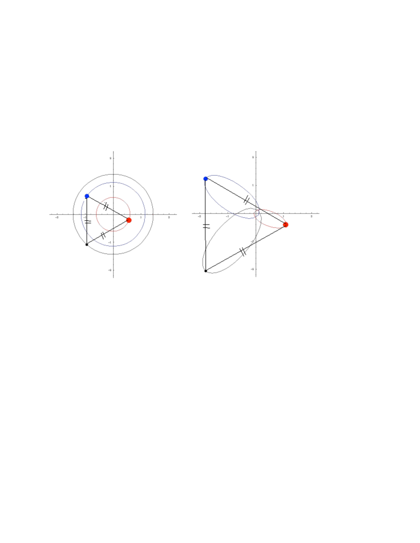
Figure 1. Lagrange solutions: the three bodies form an equilateral triangle at each instant. In the first figure the triangle rotates about its center of mass so each individual orbit is a circle. In the second the bodies travel on homothetic ellipses.

To describe their solutions observe that we can rotate and scale a triangle ${\bf q}$ by

$${\bf q}\mapsto\lambda{\bf q},\lambda\in\mathbb{C}^{*}:=\mathbb{C}\setminus{0}=\text{nonzero complex numbers}.$$

The magnitude $|\lambda|$ is the amount by which the triangle is scaled, while the argument $\theta=Arg(\lambda)$ is the amount by which the triangle is rotated. Now make the anätz (= guess) that the solution evolves solely by rotation and scaling:

(20) $${\bf q}(t)=\lambda(t){\bf q}_{0},{\bf q}_{0}\neq 0,\lambda(t)\in\mathbb{C}^{*}:=\mathbb{C}\setminus\{0\}$$

Exercise 4.

Show that ansätz (20) solves Newton’s equations (1) if and only ${\bf q}_{0,cm}:=\langle{\bf q}_{0},{\bf 1}\rangle/\Sigma m_{i}=0$ , ${\bf q}_{0}\neq 0$ and $({\bf q_{0}},\lambda(t))$ solve the two equations:

(21) $$\ddot{\lambda}=-c\frac{\lambda}{|\lambda|^{3}},$$

(22) $$\frac{c}{2}\nabla I({\bf q}_{0})=\nabla V({\bf q}_{0})$$

where $c=-V({\bf q}_{0})/I({\bf q}_{0})$.

Hint: Use form (13) of Newton’s equation, the equivariance identity $\nabla V(\lambda{\bf q})=\frac{\lambda}{|\lambda|^{3}}\nabla V({\bf q})$, and Euler’s identity for homogeneous functions.

Eq (21) is the ‘Kepler problem’ of the previous section. The second equation (22) is a Lagrange multiplier type equation asserting that ${\bf q}_{0}$ is a critical point of the function $U$, constrained to the sphere $I=I({\bf q}_{0})$. Modulo rotations and translations, there are exactly 5 such critical points, corresponding to the 3 collinear solutions found by Euler and the 2 equilateral solutions of Lagrange. They are represented by 5 points on the shape sphere. See figure 3.

6. Boundedness and the oldest problem

Let us call a solution bounded if all the interparticle distances $r_{ij}$ are bounded functions of time. For the two-body problem we saw that a solution is bounded if and only its energy is negative. A partial converse of this fact is valid in the three-body problem.

Corollary 1.

(to exercise 3) If a solution ${\bf q}(t)$ to eq (1) is bounded then its energy $H$ is negative.

Proof. If ${\bf q}(t)$ is bounded then $I(t)$ is bounded. But $U>0$ , so that if $H\geq 0$ then Lagrange-Jacobi identity $\ddot{I}=4H+2U({\bf q})$ implies $I(t)$ is strictly convex function and hence unbounded. QED

The converse is false: we know of negative energy solutions which are unbounded. (See figure 2 for one.) How false? Many people believe “very false”. (See M. Hermann ([6] ).

Problem 1.

Oldest problem in dynamical systems: Are the unbounded solutions dense within the space of negative energy solutions to the three-body problem?

When we say “the unbounded solutions are dense” we mean that the set of initial conditions whose solutions are unbounded forms a dense set. This problem is completely open, despite centuries of concerted effort. About all we know about the question is that there is an open set of unbounded solutions, and a set of positive measure consisting of bounded solutions. See figure 2 for an example of what is believed to be typical negative energy behavior in the three-body problem: two masses, say 1 and 2, form a ‘tight binary’ which runs away from the third mass, so that $r_{13},r_{23}$ tend to infinity with time.

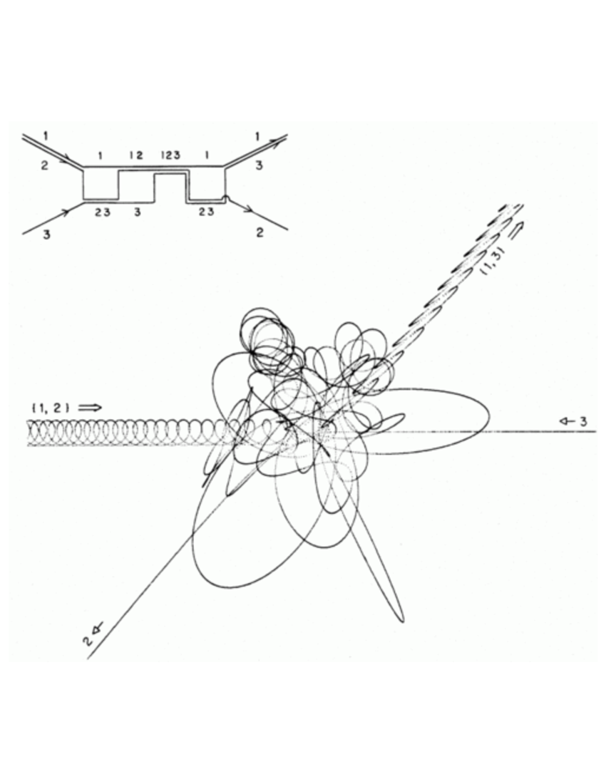
Figure 2. A typical 3 body orbit ending in a tight binary escape. Figure courtesy of Piet Hut.

***************************

PART II. Shape Space.

***********************************

7. Shape space. Main theorem.

We seek a “reduced equations”: a system of three second order ODEs which encode the three-body problem as a dynamical system on the space of congruence classes of triangles. The SSS theorem of elementary geometry asserts that this space of congruence classes is 3-dimensional with the three edge lengths $r_{12},r_{23},r_{31}$ of a triangle being coordinates. So we expect a system of 2nd order ODEs in the edge lengths. However the degenerate triangles, those with collinear vertices, form a boundary for the space of congruence classes of triangles. (We will see this boundary clearly in the theorem just below.) This boundary wreaks havoc with dynamics. We cannot write down smooth reduced differential equations for the dynamics of a congruence class valid in a neighborhood of a collinear triangle.

To salvage a reduced equation I strengthen the notion of congruence by insisting that the congruences be orientation preserving as well as distance preserving. Orientation preserving isometries are also called “rigid motions”:

Definition 2.

The group $G$ of rigid motions of the plane is the group of orientation preserving isometries of the plane.

Thus I exclude reflections from $G$. Any element of $G$ is a composition of a rotation and a translation.

Definition 3.

Two planar triangles (possibly degenerate) are ‘oriented congruent’ if there is a rigid motion taking one triangle to the other.

Definition 4.

Shape space is the space of oriented congruence classes of triangles, endowed with the quotient metric.

With this strengthening of ‘congruence” the boundary of the space of congruence classes disappears: the collinear triangles are smooth points of shape space. See Theorem 1 below.

Some words are in order regarding the meaning of “quotient metric”. The space $\mathbb{C}^{3}$ of located triangles has a Euclidean metric defined by the mass metric (eq (8)) has an associated norm $\|\cdot\|$ under which the Euclidean distance between two located triangles ${\bf q}_{1},{\bf q}_{2}$ is $\|{\bf q}_{1}-{\bf q}_{2}\|$. Our group $G$ acts on $\mathbb{C}^{3}$ by isometries relative to this distance and I denote the result of applying $g\in G$ to ${\bf q}\in\mathbb{C}^{3}$ by $g{\bf q}$. The shape space metric $d$ on the quotient by

(23) $$d([{\bf q}_{1}],[{\bf q}_{2}])=\inf_{g_{1},g_{2}\in G}\|g_{1}{\bf q}_{1}-g_{2}{\bf q}_{2})\|$$

Here $[{\bf q}_{i}]$ are the ‘shapes’, or oriented congruence classes of the located triangles ${\bf q}_{i}\in\mathbb{C}^{3}$.

Theorem 1.

(See figure 3.) Shape space is homeomorphic to $\mathbb{R}^{3}$. The quotient map from the space of located triangles to shape space is realized by a map $\pi:\mathbb{C}^{3}\to\mathbb{R}^{3}$ which is the composition a complex linear projection $\mathbb{C}^{3}\to\mathbb{C}^{2}$ (eqs (26)) and a real quadratic homogeneous map $\mathbb{C}^{2}\to\mathbb{R}^{3}$ (eq (33)). The map $\pi$ enjoys the following properties.

• A) Two triangles ${\bf q}_{1},{\bf q}_{2}\in\mathbb{C}^{3}$ are oriented congruent iff $\pi({\bf q}_{1})=\pi({\bf q}_{2})$.

• B) $\pi$ is onto.

• C) $\pi$ projects the triple collision locus onto the origin.

• D) If ${\bf w}=(w_{1},w_{2},w_{3})$ are standard linear coordinates on $\mathbb{R}^{3}$ then $w_{3}$ is the signed area of the corresponding triangle, up to a mass-dependent constant.

• E) The collinear triangle locus corresponds to the plane $w_{3}=0$.

• F) Let $\sigma:\mathbb{R}^{3}\to\mathbb{R}^{3}$ be reflection across the collinear plane: $\sigma(w_{1},w_{2},w_{3})=(w_{1},w_{2},-w_{3})$. Then the two triangles ${\bf q}_{1},{\bf q}_{2}\in\mathbb{C}^{3}$ are congruent if and only if either $\pi({\bf q}_{1})=\pi({\bf q}_{2})$ or $\pi({\bf q}_{1})=\sigma(\pi({\bf q}_{2}))$ holds.

• G) $w_{1}^{2}+w_{2}^{2}+w_{3}^{2}=(\frac{1}{2}I)^{2}$ where $I=\langle{\bf q},{\bf q}\rangle$ (see eq (14).

Remarks. E and F of the theorem say that the space of congruence classes of triangles can be identified with the closed half space $w_{3}\geq 0$ of $\mathbb{R}^{3}$. The space of collinear triangles $w_{3}=0$ form its boundary, as claimed at the beginning of this section.

7.1. The metric

Although shape space is homeomorphic to $\mathbb{R}^{3}$ it is not isometric to $\mathbb{R}^{3}$. Shape space geometry is not a Euclidean geometry. I will describe the shape space geometry in more detail below in section 10. Although the shape space geometry is not Euclidean, it is spherically symmetric, so that the geometry of each sphere $\{R=c\}$ centered at triple collision is that of the standard sphere up to a scale factor. I can identify that standard sphere with the shape sphere.

7.2. The Shape Sphere

Add scalings to the group $G$ of rigid motions in order to form the group of orientation-preserving similarities whose elements are compositions of rotations, translations and scalings.

Definition 5.

Two planar triangles are ‘oriented similar’ if there is an orientation-preserving similarity taking one to the other.

Definition 6.

The shape sphere is the resulting quotient space of the space of located triangles $\mathbb{C}^{3}\setminus\mathbb{C}{\bf 1}$, after the triple collisions $\mathbb{C}{\bf 1}$ have been deleted.

In other words, the shape sphere is the space of oriented similarity classes of planar triangles where I do not allow all three vertices of the triangle to coincide.

Figure 3. The shape sphere, centered on triple collision.

Now $\pi(\lambda{\bf q})=\lambda^{2}\pi({\bf q})$ for $\lambda$ real. It follows that the shape sphere can be realized as the space of rays through the origin in $\mathbb{R}^{3}$. This space of rays can in turn be identified with the unit sphere $\|{\bf w}\|=1$ within shape space. Various special types of triangles, including the five families of solutions of Euler and Lagrange are encoded on this sphere as indicated in figure 3.

8. Forming the Quotient. Proving Theorem 1.

Recall that a vector in $\mathbb{C}^{3}$ represent the vertices of a planar triangle, with the ith component being the ith vertex in $\mathbb{C}\cong\mathbb{R}^{2}$. Translation of such a triangle ${\bf q}=(q_{1},q_{2},q_{3})\in\mathbb{C}^{3}$ by $c\in\mathbb{C}$ sends ${\bf q}$ to the located triangle ${\bf q}+c{\bf 1}$, where ${\bf 1}=(1,1,1)$. Rotation by $\theta$ radians about the plane’s origin sends ${\bf q}$ to $e^{i\theta}{\bf q}=(e^{i\theta}q_{1},e^{i\theta}q_{2},e^{i\theta}q_{3})$. Scaling the plane by a positive factor $\rho$ corresponds to multiplication by the real number $\rho$ and so sends the triangle ${\bf q}$ to $\rho{\bf q}=(\rho q_{1},\rho q_{2},\rho q_{3})$. See figure 4.

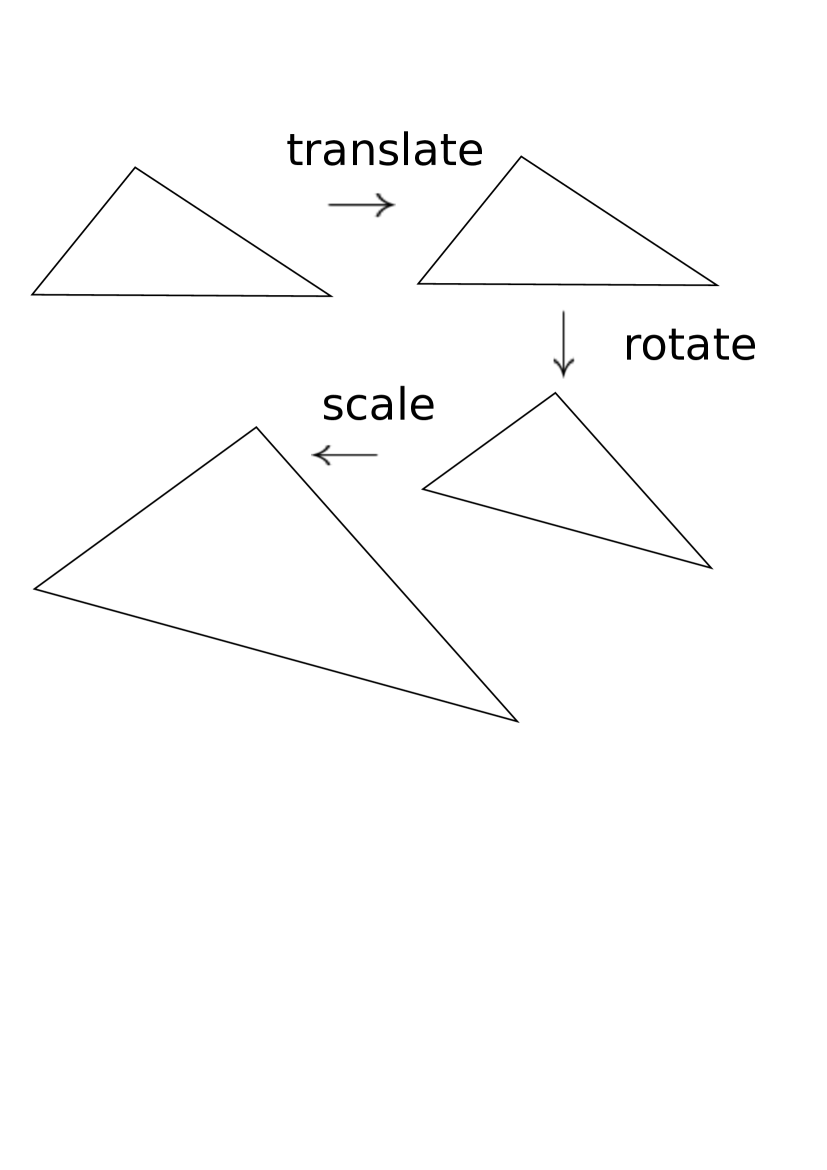
Figure 4. Translating, Rotating and Scaling a Triangle

Shape space is the quotient of $\mathbb{C}^{3}$ by the action of the group $G$ generated by translation and rotation. We form this quotient in two steps, translation, then rotation.

8.1. Dividing by translations

We divide by translations by using the isomorphism

$$\mathbb{C}^{3}/\mathbb{C}{\bf 1}\cong\mathbb{C}{\bf 1}^{\perp}.$$

which is a special case of

$${\mathbb{E}}/S\cong S^{\perp}$$

valid for any finite-dimensional complex vector space ${\mathbb{E}}$ with a Hermitian inner product, and any complex linear subspace $S\subset{\mathbb{E}}$. This isomorphism is a metric isomorphism. Here ${\mathbb{E}}/S$ inherits a Hermitian inner product whose distance is given by the formula 23 with the group $G$ replaced by $S$ acting on ${\mathbb{E}}$ by translation, and with the elements ${\bf q}_{i}$ in that formula being elements of ${\mathbb{E}}$. In the isomorphism the metric I use on $S^{\perp}$ is the restriction of the metric from ${\mathbb{E}}$.

In our situation $S$ is the span of ${\bf 1}$. I define

$$\mathbb{C}^{2}_{0}:={\bf 1}^{\perp}=\{{\bf q}:m_{1}q_{1}+m_{2}q_{2}+m_{3}q_{3}=0\}$$

the set of planar three-body configurations whose center of mass is at the origin. This two-dimencional complex space represents the quotient space of $\mathbb{C}^{3}$ by translations.

8.2. Jacobi coordinates: Diagonalizing the mass metric

It will be helpful to have coordinates diagonalizing the Hermitian form on $\mathbb{C}^{2}_{0}$. That form is the restriction of the mass metric on $\mathbb{C}^{3}$. Its associated real positive definite quadratic form is the moment of inertia: $I=\langle{\bf q},{\bf q}\rangle=m_{1}|q_{1}|^{2}+m_{2}|q_{2}|^{2}+m_{3}|q_{3}|^{2}$. Thus we look for coordinates $Z_{1},Z_{2}$ on our $\mathbb{C}^{2}_{0}$ such that:

(24) $$I=|Z_{1}|^{2}+|Z_{2}|^{2}\text{ whenever }{\bf q}\perp{\bf 1}$$

Jacobi found these coordinates.

Exercise 5.

Show that the vectors ${\bf 1}=(1,1,1),E_{1}=(\frac{1}{m_{1}},-\frac{1}{m_{2}},0)$ and $E_{2}=(\frac{-1}{m_{1}+m_{2}},\frac{-1}{m_{1}+m_{2}},\frac{1}{m_{3}})$ form an orthogonal ( but not neccessarily orthonormal) basis relative to the mass inner product on $\mathbb{C}^{3}$.

The corresponding coordinates $\langle{\bf q},{\bf 1}\rangle,\langle{\bf q},E_{1}\rangle,\langle{\bf q},E_{2}\rangle$ are orthogonal coordinates for $\mathbb{C}^{3}$.

Definition 7.

The coordinates $\langle{\bf q},E_{1}\rangle=q_{1}-q_{2}:=Q_{12}$ and $\langle{\bf q},E_{2}\rangle=q_{3}-\frac{m_{1}q_{1}+m_{2}q_{2}}{m_{1}+m_{2}}$ are called Jacobi coordinates for $\mathbb{C}^{2}_{0}:=\{{\bf q}\in\mathbb{C}^{3}:{\bf q}_{cm}=0\}$ relative to the partition $\{12;3\}$ of our three masses.

Jacobi coordinates are indicated in figure 5.

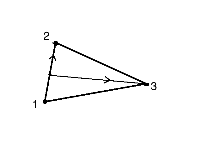
Figure 5. Jacobi vectors.

Normalizing the Jacobi coordinates yields our desired unitary diagonalizing coordinates $Z_{i}=\langle{\bf q},e_{i}\rangle,i=1,2$ for $\mathbb{C}^{2}_{0}$ where $e_{i}=E_{i}/\|E_{i}\|$. We compute

(25) $$Z_{1}=\mu_{1}(q_{1}-q_{2})\qquad Z_{2}=\mu_{2}(q_{3}-\frac{m_{1}q_{1}+m_{2}q_{2}}{m_{1}+m_{2}})$$

with $\frac{1}{\mu_{1}^{2}}=\|E_{1}\|^{2}=\frac{1}{m_{1}}+\frac{1}{m_{2}}$ and $\frac{1}{\mu_{2}^{2}}=\|E_{2}\|^{2}=\frac{1}{m_{3}}+\frac{1}{m_{1}+m_{2}}$. These normalized Jacobi coordinates define the complex linear projection

(26) $$\pi_{tr}:\mathbb{C}^{3}\to\mathbb{C}^{2}\qquad\pi_{tr}(q_{1},q_{2},q_{3})=(Z_{1},Z_{2})$$

which realizes the metric quotient of $\mathbb{C}^{3}$ by translations.

8.3. Dividing by rotations

It remains to divide $\mathbb{C}^{2}_{0}$ by the action of rotations. A rotation by $\theta$ radians acts on $\mathbb{C}^{2}_{0}$ by complex scalar multiplication by the unit modulus complex number $e^{i\theta}$. For example, such a rotation acts on the triangle’s vertices $q_{j}$ by $q_{j}\mapsto e^{i\theta}q_{j}$ so it acts on the triangle edges coordinates $Q_{jk}:=q_{j}-q_{k}$ by $Q_{jk}\mapsto e^{i\theta}Q_{jk}$. Consequently it acts on the normalized Jacobi coordinates by $(Z_{1},Z_{2})\mapsto(e^{i\theta}Z_{1},e^{i\theta}Z_{2})$.

Some generality perhaps clarifies the situation. Let $\mathbb{V}$ be a two-dimensional complex Hermitian space, like our $\mathbb{C}^{2}_{0}$ and $(Z_{1},Z_{2})$ be Hermitian orthonormal coordinates on $\mathbb{V}$. Then the rotation group $S^{1}=\{e^{i\theta},0\leq\theta\leq 2\pi\}$ of unit complex numbers acts on $\mathbb{V}$ by scalar multiplication, by $(Z_{1},Z_{2})\mapsto(e^{i\theta}Z_{1},e^{i\theta}Z_{2})$ as above. We will show that the quotient space $\mathbb{V}/S^{1}$ is homeomorphic to $\mathbb{R}^{3}$ and we will work out the metric on it. This $\mathbb{R}^{3}$ is our shape space.

Observe that the functions $Z_{i}\bar{Z}_{j}$, $i,j=1,2$ remain unchanged under rotation. We put them together into a 2 by 2 Hermitian matrix:

(27) $$\Phi(Z_{1},Z_{2})=\left(\begin{array}[]{cc}|Z_{1}|^{2}&Z_{1}\bar{Z}_{2}\\ \bar{Z}_{1}Z_{2}&|Z_{2}|^{2}\end{array}\right)=A.$$

Or

(28) $$\Phi({\bf Z})={\bf Z}^{t}{\bf Z}^{*}$$

where

$${\bf Z}=(Z_{1},Z_{2})\qquad;{\bf Z}^{t}=\left(\begin{array}[]{c}Z_{1}\\ Z_{2}\end{array}\right);\qquad{\bf\bar{Z}}=(\bar{Z}_{1},\bar{Z}_{2})$$

From the factorization (28) we see: $\Phi({\bf Z}){\bf Z}^{t}=(|Z_{1}|^{2}+|Z_{2}|^{2}){\bf Z}^{t}$ while $\Phi({\bf Z}){\bf W}^{t}=0$ for ${\bf W}\perp{\bf Z}$. Thus $\Phi(Z_{1},Z_{2})$ is the matrix of orthogonal projection onto the complex line spanned by ${\bf Z}$ (assuming ${\bf Z}\neq{\bf 0}$) multiplied by $\|{\bf Z}\|^{2}$. Now two nonzero vectors ${\bf Z},{\bf U}$ are related by rotation if and only if they span the same complex line and their lengths are equal. It follows that the image of $\Phi$ is an accurate rendition of the quotient space $\mathbb{V}/S^{1}$, with $\Phi$ being the quotient space. What is the image of $\Phi$? Well, we have just seen that it consists of the Hermitian matrices of rank $1$ whose nonzero eigenvalue is positive (corresponding to $\|{\bf Z}\|^{2}$), together with the zero matrix (corresponding to ${\bf Z}=0$). In terms of the determinant and trace these conditions on $A$ are $det(A)=0$ and $tr(A)\geq 0$. Let us coordinatize Hermitian matrices by

(29) $$A=\left(\begin{array}[]{cc}w_{4}+w_{1}&w_{2}+iw_{3}\\ w_{2}-iw_{3}&w_{4}-w_{1}\end{array}\right)\;,w_{j}\text{ real}.$$

So that $det(A)=w_{4}^{2}-w_{1}^{2}-w_{2}^{2}-w_{3}^{2}$ and $tr(A)=w_{4}$. The discussion we have just had proves:

Proposition 2.

The image of the map $\Phi$ is the cone of two by two Hermitian matrices $A$ as above (eq 29) satisfying

(30) $$w_{4}^{2}-w_{1}^{2}-w_{2}^{2}-w_{3}^{2}=0$$

and

(31) $$w_{4}\geq 0$$

This cone realizes the quotient $\mathbb{V}/S^{1}=\mathbb{C}^{2}/S^{1}$ with $\Phi$ implementing the quotient map $\mathbb{V}\to\mathbb{V}/S^{1}$.

Now map the real 4 dimensional space of Hermitian matrices to $\mathbb{R}^{3}$ onto $\mathbb{R}^{3}$ by projecting out the trace part $w_{4}$ :

$$(w_{1},w_{2},w_{3},w_{4})\mapsto pr(w_{1},w_{2},w_{3},w_{4})=(w_{1},w_{2},w_{3}).$$

The restriction of this projection to our cone (eqs (30), (31) is a homeomorphism onto $\mathbb{R}^{3}$. Indeed solve the cone equations for $w_{4}$ to find $w_{4}=+\sqrt{w_{1}^{2}+w_{2}^{2}+w_{3}^{2}}$ and hence the the inverse of the restricted projection is $(w_{1},w_{2},w_{3})\mapsto(w_{1},w_{2},w_{3},\sqrt{w_{1}^{2}+w_{2}^{2}+w_{3}^{2}})$ We have proved:

Proposition 3.

The map

(32) $$\pi^{rot}=pr\circ\Phi:\mathbb{C}^{2}\to\mathbb{R}^{3}$$

given by

(33) $$\pi^{rot}(Z_{1},Z_{2})=(\frac{1}{2}(|Z_{1}|^{2}-|Z_{2}|^{2},Re(Z_{1}\bar{Z}_{2}),Im(Z_{1}\bar{Z}_{2})=(w_{1},w_{2},w_{3})$$

realizes $\mathbb{R}^{3}$ as the quotient space of $\mathbb{C}^{2}$ by the rotation group $S^{1}$.

Remark. The restriction of the map (32) to the sphere $w_{4}=1$ is the famous Hopf map from the three-sphere to the two-sphere.

8.4. Proof of theorem 1.

We compose the projections $\pi_{tr}$ of eq (26) and the map $\pi^{rot}$ immediately above. The first realizes the quotient by translations and the second realizes the quotient by rotations so together they realize the full quotient by the group of rigid motions. This establishes A and B of the theorem. Property C, that the only triangles sent to $0\in\mathbb{R}^{3}$ are the triple collision triangles ${\bf q}=(q,q,q)$ follows directly from the formulae for $\pi^{rot}$ and $\pi_{tr}$. Indeed, the only point of $\mathbb{C}^{2}$ mapped to $0$ by $\pi_{tr}$ is the origin $0$, and the only points of $\mathbb{C}^{3}$ mapped to the origin by $\pi_{tr}$ are the triple collision points.

We verify property D which says $w_{3}$ is a mass-dependent constant times the oriented area of the triangle. We have $w_{3}=-Z_{1}\wedge Z_{2}$. Recall that the wedge (eq (16)) $z\wedge w=Im(\bar{z}w)$ represents the oriented area of the parallelogram whose edges are$z=x+iy$ and $w=u+iv$. Thus the oriented area of our triangle is $\frac{1}{2}(Q_{21})\wedge(Q_{31})$ where we write $Q_{ij}=q_{i}-q_{j}$ for the edge connecting vertex j to vertex i. We have $Z_{1}=\mu_{1}Q_{12}$ and $Z_{2}=\mu_{2}(p_{1}Q_{31}+p_{2}Q_{32})$ where $p_{1}=m_{1}/(m_{1}+m_{2})$ and $p_{2}=m_{2}/(m_{1}+m_{2})$ so that $p_{1}+p_{2}=1$. Use $Q_{12}+Q_{23}+Q_{31}=0$ and $Q_{ij}=-Q_{ji}$ to compute that $Z_{2}=\mu_{2}(Q_{31}-p_{2}Q_{12})$. Now the wedge operation is skew symmetric: $Q_{12}\wedge Q_{12}=0$. It follows that $w_{3}=-\mu_{1}\mu_{2}\frac{1}{2}Q_{12}\wedge Q_{31}=+\mu_{1}\mu_{2}\frac{1}{2}Q_{21}\wedge Q_{31}$ as desired.

Property E follows immediately from property D. To establish property F regarding the operation of reflection on triangles, observe that we can reflect triangle ${\bf q}$ by changing all vertices $q_{i}$ to $\bar{q}_{i}$ which in turn changes $(Z_{1},Z_{2})$ to its conjugate vector $(\bar{Z}_{1},\bar{Z}_{2})$. This conjugation operation leaves $w_{1}$ and $w_{2}$ unchanged and changes $w_{3}$ to $-w_{3}$: the oriented area flips sign.

Property G is a computation. Observe from eqs (27, 29) that $w_{4}=\frac{1}{2}I$ and recall the cone condition eq (30): $w_{4}^{2}=w_{1}^{2}+w_{2}^{2}+w_{3}^{2}$.

QED

9. Mechanics via Lagrangians.

One of my goals here is to write down the reduced equations encoding Newton’s equations (1) on shape space. My strategy for achieving this goal is to push the least action principle for the three-body problem down from the space $\mathbb{C}^{3}$ of located triangles to our shape space $\mathbb{R}^{3}$. We begin by stating the least action principle.

Any classical mechanical system can be succinctly encoded by its Lagrangian $L$. ([1] or [11]),

(34) $$L=K-V$$

the difference of its kinetic $(K)$ and potential $(V)$ energies. (Recall that the energy is the sum $K+V$.) Integrating the Lagrangian over a path $c$ in the configuration space of the mechanical system defines that path’s action :

$$A[c]=\int_{c}Ldt=\int_{a}^{b}L(c(t),\dot{c}(t))dt.$$

In this last expression we have taken $c$ to be parameterized by the time interval $[a,b]$ so that $c:[a,b]\to Q$ where $Q$ denotes the configuration space. The principle of least action asserts that a curve satisfies Newton’s equations if and only if $c$ minimizes $A$ among all paths $\gamma:[a,b]\to Q$ for which $c(a)=\gamma(a)$ and $c(b)=\gamma(b)$.

The principle is not a theorem but rather it is a guiding principle. To turn the principle into a theorem requires careful wording and more hypothesis. Here is such a theorem in the case of the three-body problem.

Theorem 2.

If a curve $c:[0,T]\to\mathbb{C}^{3}$ minimizes the action among all curves $\gamma:[0,T]\to\mathbb{C}^{3}$ sharing its endpoints and if $c$ has no collisions on the open interval $(0,T)$ then $c$ solves Newton’s equations on $(0,T)$. Conversely, if a curve $c:[a,b]\to\mathbb{C}^{3}$ satisfies Newton’s equations then there is an $\epsilon>0$ such that the restriction $c|_{[r,s]}$ of $c$ to any subinterval $[r,s]$ of size $s-r\leq\epsilon$ mininimizes the action among all curves $\gamma:[r,s]\to\mathbb{C}^{3}$ sharing its endpoints: $\gamma(r)=c(r),\gamma(s)=c(s)$.

An analogous theorem holds regarding the principle of least action in situations much more general than that of the three-body problem. For example, we can take the configuration space $Q=\mathbb{R}^{n}$ a real vector space and $K$ the squared norm associated to any inner product on $\mathbb{R}^{n}$. We view $K$ as being applied to velocities $v\in\mathbb{R}^{n}$. Take $V:\mathbb{R}^{n}\to\mathbb{R}$ any smooth function. Then the Lagrangian is $L(x,v)=K(v)-V(x)$ which is a function on the phase space $\mathbb{R}^{n}\times\mathbb{R}^{n}$. Newton’s equations are the 2nd order differential equation

(35) $$\ddot{c}=-\nabla V(c).$$

for curves $c$ on $\mathbb{R}^{n}$. In these equations $\nabla$ is the gradient associated to the kinetic energy $K$, as described in analogy to eq (12). More generally we can take $Q$ to be any Riemannian manifold with $K$ the associated kinetic energy ($\frac{1}{2}\Sigma g^{ij}(q)p_{i}p_{j}$. Here the coordinate expression of the Riemannian metric is $g_{ij}$. And take $V:Q\to\mathbb{R}$ any smooth function. Then the $\nabla$ of Newton’s equations above is the covariant derivative and the second derivative of $c$ becomes the second covariant derivative of the curve.

9.1. Euler-Lagrange Equations

Let $\xi^{a},a=1,\ldots,n$ be coordinates on our configuration space $Q$. Then the Lagrangian is a function of the $\xi^{a}$ and its formal time derivatives $\dot{\xi}^{a}$:

$$L=L(\xi^{1},\ldots,\xi^{n},\dot{\xi}^{1},\ldots,\dot{\xi}^{n}).$$

The Euler-Lagrange equations :

(36) $$\frac{d}{dt}({{\partial L}\over{\partial\dot{\xi}^{a}}})={{\partial L}\over{\partial\xi^{a}}}$$

are ODEs which a path $\xi^{a}=\xi^{a}(t)$ must satisfy if it minimizes the action. They are Newton’s equations expressed in the new coordinates $\xi_{a}$.

Words are in order regarding the left-hand side of the EL equations (36). We compute ${{\partial L}\over{\partial\dot{\xi}^{a}}}$ by treating $\xi^{a}$ and $\dot{\xi}^{a}$ as independent variables. The resulting ${{\partial L}\over{\partial\dot{\xi}^{a}}}$ is now a function of the variables $\xi^{a},\dot{\xi}^{a}$. We then compute $\frac{d}{dt}({{\partial L}\over{\partial\dot{\xi}^{a}}})$ by formally replacing the independent variables $\xi^{a},\dot{\xi}^{a}$ in ${{\partial L}\over{\partial\dot{\xi}^{a}}}$ by an alleged curve $\xi^{a}(t)$ and its time derivatives $\dot{\xi}^{a}(t)$ so as to get a function of time which we finally differentiate formally using the chain rule.

Exercise 6.

Suppose that $K=\frac{1}{2}\Sigma g_{ab}\dot{\xi}^{a}\dot{\xi}^{b}$ and that $V=V(\xi^{1},\ldots,\xi^{n})$.Verify that Newton’s equations (13) are equivalent to the Euler-Lagrange equations with respect to the coordinates $\xi^{a}$.

One of the beauties and the powers of the action principle is it is coordinate-independent. If a path minimizes the action then it does not matter what coordinate system we use to express that path. The path still minimizes the action and so satisfies the Euler-Lagrange equations in that coordinate system.

Exercise 7.

For $Q=\mathbb{R}^{2}$ and $L=\frac{1}{2}(\dot{x}^{2}+\dot{y}^{2})$ the EL equations are those whose solutions are straight lines travelled at constant speed. Rewrite $L$ in polar coordinates $r,\theta$ and write down the corresponding Euler-Lagrange equations, thus deriving the equations of a straight line in polar coordinates.

9.2. Reducing the least action principle

The curves competing in the least action principle as we stated it are subject to boundary conditions : they connect two fixed points of the configuration space $\mathbb{C}^{3}$ of located triangles. Replace the two points by two oriented congruence classes to get new boundary conditions: the competing curves connect two fixed oriented congruence classes of configuration space. If we remember that an oriented congruence class is represented by a point of shape space we arrive at an action principle for shape space.

Shape space action principle. Fix two shapes ${\bf w}_{0},{\bf w}_{1}$ in the shape space $\mathbb{R}^{3}$. Suppose that ${\bf q}(t)\in\mathbb{C}^{3},0,\leq t\leq T$ minimizes the standard action (34) among all curves in the space $\mathbb{C}^{3}$ of located triangles which join the corresponding oriented congruence classes $\Sigma_{0}=\pi^{-1}({\bf w}_{0}),\Sigma_{1}=\pi^{-1}({\bf w}_{1})\subset\mathbb{C}^{3}$ in time $T$. Then we will say that its projected curve $\pi({\bf q}(t))\in\mathbb{R}^{3}$ minimizes the shape space action among all curves connecting the endpoints ${\bf w}_{0},{\bf w}_{1}$ in time $T$.

Consider an analogous change of boundary conditions for the simplest action functional in the plane, the length functional. Instead of minimizing the length of curves amongst all curves connecting two fixed points in the plane , replace these two points by two disjoint circles $\Sigma_{0}$ and $\Sigma_{1}$. We know that the minimizer will be a line segment which is perpendicular to both $\Sigma_{0}$ and $\Sigma_{1}$ at its endpoints. More generally, for a Lagrangian on $\mathbb{R}^{n}$ of the general form (34) , if we replace the fixed endpoint minimization problem with the problem of minimizing the action among all curves connecting two given subspaces $\Sigma_{0},\Sigma_{1}\subset\mathbb{R}^{n}$ then we induce a derivative condition at the endpoints: namely the extremal curves, in addition to satisfying the Euler-Lagrange equations must hit their targets orthogonally: $\dot{c}(0)\perp\Sigma_{0}$ at $c(0)$ and $\dot{c}(T)\perp\Sigma_{1}$ at $c(T)$. We call this added condition “ first variation orthogonality”.

Returning to our situation where $\Sigma_{0}=\pi^{-1}({\bf w}_{0}),\Sigma_{1}=\Sigma_{1}=\pi^{-1}({\bf w}_{1})$ are oriented congruence classes in $\mathbb{C}^{3}=\mathbb{R}^{6}$. We will interpret first variation orthogonality in mechanical terms. We may sweep out all of $\Sigma_{0}$ by applying variable rigid motions $g\in G$ to a single point ${\bf q}_{0}\in\Sigma_{0}$. In set theory notation: $\Sigma_{0}=\{g{\bf q}_{0}:g\in G\}$. Set $g=g(t)$ to form paths ${\bf q}(t)=g(t){\bf q}_{0}$ in $\Sigma_{0}$ and differentiate these paths, alternately taking $g(t)$ to be a curve of translations or a curve of rotations. By this means we see that the tangent space $T_{{\bf q}_{0}}\Sigma_{0}$ to $\Sigma_{0}$ at ${\bf q}_{0}$ is spanned by two subspaces, $\{\dot{c}{\bf 1},\dot{c}\in\mathbb{C}\}$ for translations, and $\{i\dot{\theta}{\bf q}_{0}:\dot{\theta}\in\mathbb{R}\}$:

(37) $$T_{{\bf q}_{0}}\Sigma_{0} =\text{infinitesimal rigid motions}$$

(38) $$=\text{(translational)}+\text{(rotational)}$$

(39) $$=span_{\mathbb{C}}{\bf 1}+span_{\mathbb{R}}(i{\bf q})$$

The first variation orthogonality condition is thus that our extremal ${\bf q}(t)$ be orthogonal to both the translation and rotational spaces: $\langle{\bf 1},{\bf\dot{q}}(0)\rangle=0$ $\langle i\dot{\theta}{\bf q}(0),{\bf\dot{q}}(0)\rangle=0$. But as we saw in eqns (17, 15) these orthogonality conditions are equivalent to the assertions that the linear and angular momentum are zero at ${\bf q}_{0}$. (The inner product is the real part of the Hermitian one and $Im(\langle{\bf q},{\bf\dot{q}}\rangle)=Re(\langle i{\bf q},{\bf\dot{q}}\rangle$.) We summarize

Lemma 1.

The curve ${\bf q}(t)$ in $\mathbb{C}^{3}$ is orthogonal to the oriented congruence class through ${\bf q}_{0}={\bf q}(0)$ if and only if its linear and angular momentum are zero at $t=0$. (See equations (17) and ( 15).)

Now if the curve ${\bf q}(t)$ of the lemma is an extremal for our shape space action principle then it must satisfy the EL equations which are Newton’s equations. Since linear and angular momentum are conserved for solutions to Newton’s equations we have that the linear and angular momentum are identically zero all along the curve. Equivalently: if an extremal curve is orthogonal to the $G$ orbit $\Sigma_{0}$ through one of its points, then it is orthogonal to the group orbits $\Sigma_{t}$ through every one of its points. We have established:

Proposition 4.

The extremals for the shape space action principle are precisely those solutions to Newton’s equations whose linear and angular momentum are zero.

The proposition suggests a strategy for finding a Lagrangian $L_{shape}$ on shape space whose action miniimization is equivalent the shape space action principle. The Euler-Lagrange equations for $L_{shape}$ will be our desired reduced equations. Break up kinetic energy into

(40) $$K=\text{translational part}+\text{ rotational part }+\text{ shape part}.$$

We have just agreed that the translation and rotational part of the kinetic energy must be zero along our shape extremals corresponding to the fact that they are orthogonal to $G$-orbits. Let us denote the last term, the shape term of the kinetic energy as $K_{shape}$. Thus

(41) $$L_{shape}=K_{shape}-V$$

is the shape Lagrangian. It remains to express $K_{shape}$ in terms of shape coordinates $w_{i}$ and their time derivatives $\dot{w}_{i}$ and $V$ in terms of the $w_{i}$. We find these expressions in the next three sections.

9.3. Shape kinetic energy

The decomposition (40) applied to veloicites is sometimes called the “Saari decomposition”: (LABEL:Saari, LABEL:Chenciner).

(42) $$\dot{\bf q} =(\text{translational part}+\text{ rotational part })+\text{ shape part}.$$

(43) $$=T_{q}(Gq)\hskip 17.07182pt\oplus\hskip 73.97733pt(T_{q}(Gq))^{\perp}$$

(44) $$=\text{vertical}+\text{horizontal}$$

In the differential geometry of bundles such a splitting is known as a “‘vertical- horizontal” splitting in the theory of bundles, $T_{q}(Gq)$ forms the “vertical space” and its orthogonal complement $T_{q}(Gq))^{\perp}$ forming the “horizontal space”. This decomposition, which depends on the base point ${\bf q}$ at which the velocity is attached, is orthogonal and leads to

Proposition 5.

Suppose that the center of mass of our located triangle is zero. Then the Saari decomposition, eq (40) above is

$$K=\frac{1}{2}\frac{\|{\bf P}\|^{2}}{M}+\frac{1}{2}\frac{J^{2}}{I}+\frac{1}{2}\frac{\|{\bf\dot{w}}\|^{2}}{I}$$

where ${\bf\dot{w}}=\frac{d}{dt}\pi({\bf q}(t))$and $P=P({\bf\dot{q}}),J=J({\bf q},{\bf\dot{q}})$ are the linear and angular momenta (eq 15, 17). In particular

(45) $$K_{shape}=\frac{1}{2}\frac{\|{\bf\dot{w}}\|^{2}}{I}=\frac{1}{2}\frac{\|{\bf\dot{w}}\|^{2}}{2\sqrt{\|{\bf w}\|}}$$

Proof. A real basis for the two-dimensional translational part of the motion consists of ${\bf 1},i{\bf 1}$ and a real basis for the one-dimensional rotational part is $i{\bf q}$. The rotational part is orthogonal to the translational part since the center of mass is given by $\frac{1}{M}\langle{\bf q},{\bf 1}\rangle$ which we have supposed to be zero. ($M=\langle{\bf 1},{\bf 1}\rangle=m_{1}+m_{2}+m_{3}$ is the total mass.) Hence ${\bf 1},i{\bf 1},i{\bf q}$ is an orthogonal basis for the vertical part, $T_{q}(Gq)$. Normalize to get the orthonormal basis

$$e_{1},e_{2},e_{3}={\bf 1}/\sqrt{M},i{\bf 1}/\sqrt{M};i{\bf q}/\sqrt{I}$$

for the vertical part of the motion. Let ${\bf\dot{q}}\in\mathbb{C}^{3}$ be an arbitrary vector based at the located triangle ${\bf q}_{0}\in\mathbb{C}^{3}$ and expand this vector as an orthogonal direct sum to get the following quantitative form of the Saari decomposition eq (44)

$${\bf\dot{q}}=\langle{\bf\dot{q}},e_{1}\rangle_{\mathbb{R}}e_{1}+\langle{\bf\dot{q}},e_{2}\rangle_{\mathbb{R}}e_{2}+\langle{\bf\dot{q}},e_{3}\rangle_{\mathbb{R}}e_{3}+\text{(shape)}.$$

The first three terms form the vertical part of the velocity in eq (44) while the final (shape) part is, by definition, orthogonal to the first three terms and forms the horizontal part. Squaring lengths and using the orthonormality of $e_{1},e_{2},e_{3}$ we find that

$$\langle{\bf\dot{q}},{\bf\dot{q}}\rangle=|P|^{2}/M+J^{2}/I+\text{shape}^{2}.$$

It remains to show that $|\text{shape}|^{2}=\frac{\|\dot{\bf w}\|^{2}}{I}$. In other words, we need to show that

(46) $$\|{\bf\dot{w}}\|^{2}=\|{\bf q}|^{2}\|{\bf\dot{q}}\|^{2}\text{ if }P({\bf\dot{q}})=0,J({\bf q},{\bf\dot{q}})=0\text{ and }{\bf\dot{w}}=D\pi_{\bf q}({\bf\dot{q}}).$$

To this end, write out the map $\pi^{rot}$ in real coordinates, using $Z_{j}=x_{j}+iy_{j}$, ${\bf q}=(Z_{1},Z_{2})=(x_{1},y_{1},x_{2},y_{2}).$ We have $\pi^{rot}((x_{1},y_{1},x_{2},y_{2})=(\frac{1}{2}(x_{1}^{2}+y_{1}^{2}-x_{2}^{2}-y_{2}^{2},x_{1}x_{2}+y_{1}y_{2},x_{2}y_{1}-x_{1}y_{2}).$ Compute the Jacobian:

$$D\pi^{rot}_{\bf q}=\left(\begin{array}[]{cccc}x_{1}&y_{1}&-x_{2}&-y_{2}\\ x_{2}&y_{2}&x_{1}&y_{1}\\ -y_{2}&x_{2}&y_{1}&-x_{1}\end{array}\right).$$

and set

$$L=D\pi^{rot}_{\bf q}.$$

The three rows of $L$ are orthogonal and each has length $\|{\bf q}\|^{2}$. It follows that

$$LL^{T}=\|{\bf q}\|^{2}Id.$$

Now the kernel of $L$ is spanned by $e_{1},e_{2},e_{3}$ since $\pi$ is invariant under rotations and translations. Thus the image of $L^{T}$ is the orthogonal complement to $e_{1},e_{2},e_{3}$ – the subspace “(shape)” above. Consequently any vector ${\bf\dot{q}}$ of the form required in eq (46) can be written ${\bf\dot{q}}=L^{T}{\bf v}$ for some ${\bf v}\in\mathbb{R}^{3}$. Thus:

(47) $$\|{\bf\dot{q}}\|^{2} =\langle L^{T}{\bf v},L^{T}{\bf v}\rangle$$

(48) $$=\langle{\bf v},LL^{T}{\bf v}\rangle$$

(49) $$=\langle{\bf v},\|{\bf q}\|^{2}{\bf v}\rangle$$

(50) $$=\|{\bf q}\|^{2}\|{\bf v}\|^{2}$$

And ${\bf\dot{w}}=L{\bf\dot{q}}$ so that ${\bf\dot{w}}=LL^{T}{\bf v}=\|{\bf q}\|^{2}{\bf v}$. We get that $\|{\bf\dot{w}}\|^{2}=\|{\bf q}\|^{4}\|{\bf v}\|^{2}=\|{\bf q}\|^{2}\|{\bf\dot{q}}\|^{2}$. Thus $\|{\bf\dot{q}}\|^{2}=\|{\bf\dot{w}}\|^{2}/\|{\bf q}\|^{2}$. Use $I=\|{\bf q}\|^{2}$ and $I=2\sqrt{\|{\bf w}\|}$ (property G of theorem 1).

10. Shape Space metric

Definition 8.

The shape space metric is the twice the shape space kinetic energy $K_{shape}$, viewed as a Riemannian metric on shape space, so a bilinear quadratic form on velocities depending smoothly on ${\bf w}\in\mathbb{R}^{3}$.

We have seen in the previous proposition that the shape space metric is given by

(51) $$ds_{shape}^{2}=\frac{dw_{1}^{2}+dw_{2}^{2}+dw_{3}^{2}}{2\sqrt{w_{1}^{2}+w_{2}^{2}+w_{3}^{2}}}$$

Like any Riemannian metric, this metric induces a distance function on shape space. We recall how this distance function is defined. First define the length $\ell$ of a path in shape space to be $\ell(c)=\int_{c}ds_{shape}:=\int_{a}^{b}\sqrt{2K_{shape}}dt$. Now define the distance between two points as the infimum of the lengths of all paths that join the two points. In other words, the shape space length is the action relative to the Lagrangian $\sqrt{2K_{shape}}$ and the shape space distance between two points is realized by an action-minimizing curve which joins the points. We call such a minimizer a geodesic.

Reparameterizing a curve does not change its length. When we parameterized a curve by a constant multiple of arclength then we are insisting that $K_{shape}$ is constant along the curve. By a well-known argument involving the Cauchy-Schwartz inequality, the length minimizing curves which are so parameterized are precisely the curves which minimize $\int K_{shape}dt$. Now the shape space action principle holds for $K$ in place of $K-V$, and the corresponding reduced Lagrangian is $K_{shape}$. The geodesics for $K$ are straight lines in $\mathbb{C}^{3}$. Putting together these observations we have proved the assertions of the first two sentences of:

Theorem 3.

The distance function defined by the Riemannian metric agrees with the shape space distance of eq (23) . Its geodesics are the projections by $\pi:\mathbb{C}^{3}\to\mathbb{R}^{3}$ of horizontal lines in $\mathbb{C}^{3}$. Each plane $\Pi:Aw_{1}+Bw_{2}+Cw_{3}=0$ through the origin is totally geodesic: a geodesic which starts on $\Pi$ initially tangent to $\Pi$, lies completely in the plane $\Pi$. The restriction of the Riemannian metric to such a plane $\Pi$, when expressed in standard Euclidean polar coordinates $(r,\theta)$ on that plane, has the form

$$ds^{2}_{shape}|_{\Pi}=dr^{2}+\frac{1}{4}r^{2}d\theta^{2}.$$

In order to finish the proof of this theorem, let $\ell(t)={\bf q}+t{\bf v}$ be a horizontal line passing through the point ${\bf q}\in\mathbb{C}^{2}_{0}\subset\mathbb{C}^{3},{\bf q}\neq 0$ with horizontal tangent vector ${\bf v}$. There are two possibilities for ${\bf v}$: a multiple of ${\bf q}$ or linearly independent of ${\bf q}$. In the first case, we may assume that ${\bf v}={\bf q}$ is the radial vector. (Note that this vector is horizontal.) Then $\ell$ is a radial line and $\pi(\ell)$ is the ray connecting the triple collision point $0$ to ${\bf w}=\pi({\bf q})$ (traversed twice). The distance from $0$ to ${\bf w}$ along this ray is the radial variable

$$r=dist(0,{\bf w})=\|{\bf q}\|=\sqrt{I}=\sqrt{2\|{\bf w}\|}.$$

In the second case ${\bf q}$ and ${\bf v}$ span a real horizontal two-plane $P$ in $\mathbb{C}^{3}$ which passes through $0$ and contains the line $\ell$. One computes that the projection $\Pi:=\pi(P)\subset\mathbb{R}^{3}$ is a plane (rel. the coordinates $w_{i}$) passing through $0$. However the projection $\pi(\ell)$ is not a line (relative to the linear coordinates $w_{i}$)!

We can understand the geodesic $\pi(\ell)$ in shape space by understanding the restriction $ds^{2}_{shape}|_{\Pi}$ of the shape space metric to the plane $\pi(P)$. Here is what we know so far about this metric. The radial lines are geodesics. The distance along such a radial geodesic from the triple collision point $0$ to a random point ${\bf w}\in\pi(P)$ is $r$ as given above. To dilate the metric by a factor $t>0$ we multiply ${\bf w}\in\mathbb{R}^{3}$ by $t^{2}$, since ${\bf q}\mapsto t{\bf q}$ corresponds to ${\bf w}\mapsto t^{2}{\bf w}$ under $\pi$. Finally, the metric on $\Pi$ is rotationally symmetric, since the expression (51) is rotationally invariant. From all of this information we deduce that the restricted metric as the form:

(52) $$ds^{2}_{\pi(P)}=dr^{2}+c^{2}r^{2}d\theta^{2}$$

where $(r,\theta)$ are polar coordinates on the plane and $c$ is a constant. It remains to show that $c=1/2$. With this in mind, consider the circle $r=1$ in the plane $\Pi$. Its circumference computed from the formula (eq 52) is $2\pi c$. But we can also compute its length by working up on $P\subset\mathbb{C}^{3}$. Take ${\bf q}$ and ${\bf v}$ to both be unit length and orthogonal, so an orthonormalbasis for $P$. Then the corresponding horizontal circle on $P$ is $\cos(s){\bf q}+\sin{s}{\bf v}$, $0\leq s\leq 2\pi$. But $\pi({\bf q})=\pi(-{\bf q})$, since $-{\bf q}=e^{i\pi}{\bf q}$, so that the projection of this circle closes up once we have gone half way around, from $s=0$ to $s=\pi$. Thus the projected circle on $\pi(P)=\Pi$ has the length of half a unit circle, or $\pi$. Comparing lengths we see that $c=1/2$.

Any metric of form (52) is that of a cone. We can form our $c=1/2$ cone by taking a sheet of paper and marking the midpoint of one edge to be the cone point. See figure 6.

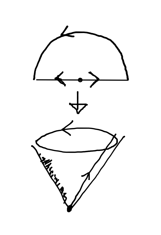
Figure 6. Folding a half-sheet of paper makes the desired cone.

Fold that edge up so the two halves touch eachother and we have a paper model of the required cone. Note that the circle of radius $r$ about the cone point has circumference $\pi r$, as required.

11. Potential on shape space.

In order to express the potential (equation (10)) in terms of the shape coordinates $w_{i}$ it suffices to express the distance $r_{ij}$ between bodies $i$ and $j$ in terms of the $w_{i}$’s. Here is the basic geometric fact that makes this computation possible:

Lemma 2.

Let $d_{ij}$ denote the shape-space distance from the point ${\bf w}$ to the ij binary collision ray. Then

$$\sqrt{\mu_{ij}}r_{ij}=d_{ij}$$

where $\mu_{ij}=m_{i}m_{j}/(m_{i}+m_{j})$.

Let ${\bf b}_{12},{\bf b}_{23},{\bf b}_{31}$ be the unit vectors in shape space whose postive span defines the corresponding binary collision ray. For example ${\bf b}_{12}$ represents the binary collision $r_{12}=0$ etc. The dot product and norm in the following lemma are the standard dot product and norm on $\mathbb{R}^{3}$.

Lemma 3.

The distance $r_{ij}$ between body $i$ and $j$ is given by

(53) $$r_{ij}^{2}={{m_{i}+m_{j}}\over{m_{i}m_{j}}}(\|{\bf w}\|-{\bf w}\cdot{\bf b}_{ij})$$

Proof of Lemma 2. We will just do the case $i,j=1,2$. Let ${\bf q}=(q_{1},q_{2},q_{3})\in\mathbb{C}^{2}_{0}$ be a centered located triangle whose projection to shape space is ${\bf w}$. Let masses 1 and 2 move towards each other along the line segment which joins them until they collide. Make the motion linear and such that their center of mass remains unchanged. Keep mass 3 fixed, so that the second Jacobi vector remains also constant. Described in Jacobi coordinates this motion is given by $((1-t)Z_{1},Z_{2}),0\leq t\leq 1$. The curve just described is a horizontal line segment and so realizes the shape space distance between its endpoints in shape space $\mathbb{R}^{3}$. One endpoint of the segement is the initial shape ${\bf w}$. The other endpoint lies on the $12$ binary collision ray.

When we view this line segment as a moving triangle in the plane, vertices 1 and 2 sweep out their entire edge $[q_{1},q_{2}]$, meeting somewhere in the middle (at their common center of mass) while vertex 3 remains fixed. From this perspective the following is no surprise.

Exercise 8.

Compute the length of this line segment relative to the mass metric to be $\sqrt{\mu_{12}}r_{12}$ where $\mu_{12}=m_{1}m_{2}/(m_{1}+m_{2})$.

Our Jacobi coordinate description of the line segment used in the proof of Lemma 2 shows that the segment hits the 12 collision locus $Z_{1}=0$ orthogonally at $t=1$. Thus this segment represents a horizontal geodesic which minimizes the distance from the shape space point ${\bf w}$ to the binary collision ray associated to ${\bf b}_{12}$. It follows that the distance between ${\bf w}$ and that collision ray is

(54) $$d_{12}=\sqrt{\mu_{12}}r_{12}$$

QED

Proof of Lemma 3. We use the conical structure of the metric ( eq (52), and Theorem 3) to compute $d_{12}$ a different way. Two linearly independent vectors ${\bf w},{\bf b}\in\mathbb{R}^{3}$ define two rays which span a plane $\Pi$ through the origin. The metric on this plane is of the form ((52) with $c=1/2$. This factor of $1/2$ implies that the shape space angle $\theta$ between the two rays is exactly half of the their Euclidean angle. In other words:

$${\bf w}\cdot{\bf b}=\|{\bf w}\|cos(\psi)\;;\psi=2\theta$$

The geometry of any two dimensional conical metric (52) is locally Euclidean. It follows that we can compute the shape space distance $d_{12}$ between ${\bf w}$ and the ray spanned by ${\bf b}_{12}$ using standard trigonometry as indicated in figure 7.

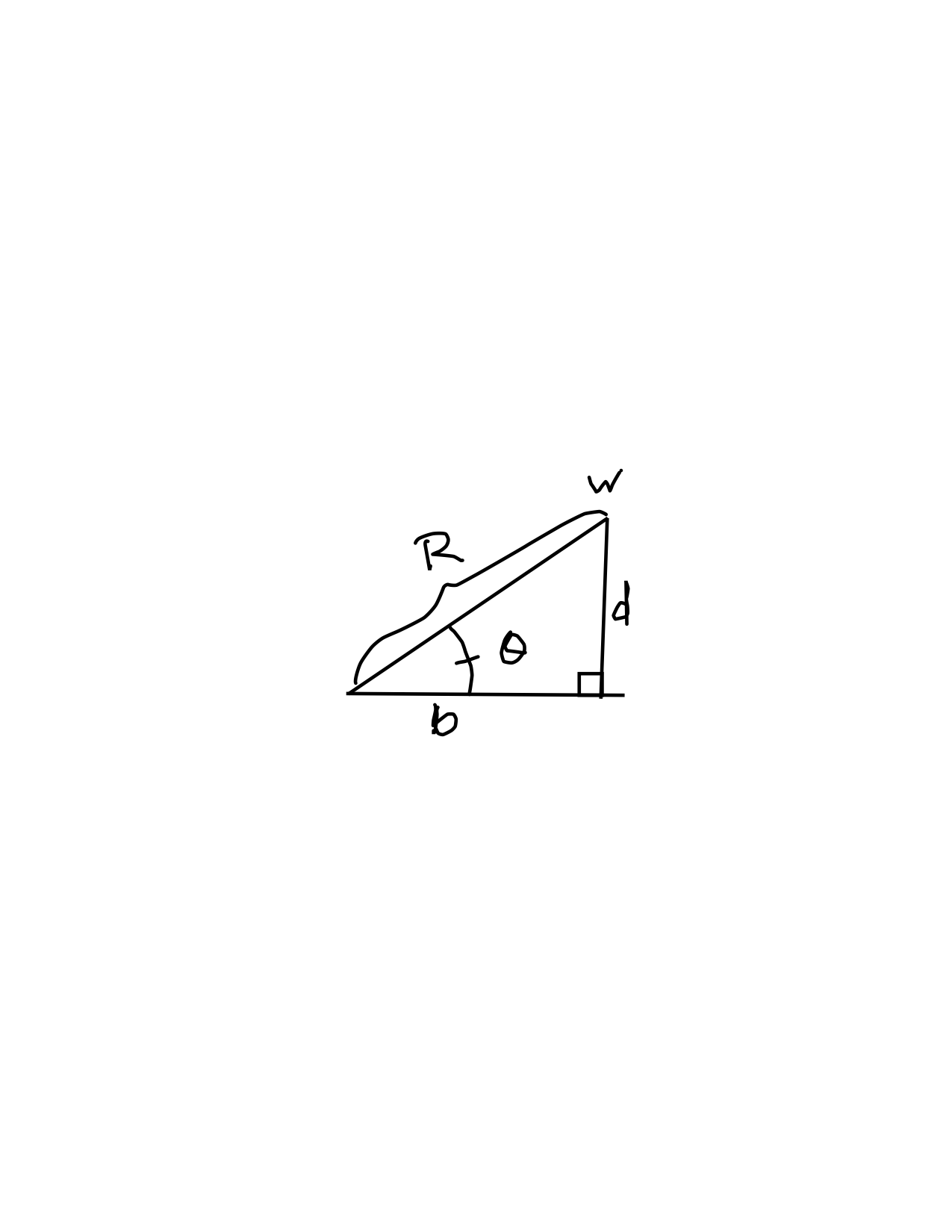
Figure 7. A Euclidean triangle allows us to compute $d=d_{12}$.

From the figure $d_{12}=r\sin(\theta)$ so that

$$d_{12}^{2}=r^{2}\sin^{2}(\theta)$$

From ${\bf w}\cdot{\bf b}_{12}=\|{\bf w}\|\cos(\psi)$, $\psi=2\theta$ and $2\|{\bf w}\|=r^{2}$ we compute that $\|{\bf w}\|-{\bf w}\cdot{\bf b}_{12}=r^{2}\sin^{2}\theta$ or

(55) $$d_{12}^{2}=\|{\bf w}\|-{\bf w}\cdot{\bf b}_{12}$$

Formula (53) in the case $i,j=1,2$ now follows immediately from this last equation and eq (54).

12. Reduced equations of Motion.

I now have written both the shape space kinetic energy (eq.( 45)) and the potential energy (eq 10) in terms of shape space variables $w_{i}$. Consequently we have the shape space Lagrangian:

(56) $$L_{shape}=\frac{1}{2}\frac{\dot{w}_{1}^{2}+\dot{w}_{2}^{2}+\dot{w}_{3}^{2}}{2\sqrt{w_{1}^{2}+w_{2}^{2}+w_{3}^{2}}}+\frac{c_{12}}{d_{12}}+\frac{c_{23}}{d_{23}}+\frac{c_{13}}{d_{13}}$$

Here $c_{ij}=m_{i}m_{j}\sqrt{\mu_{ij}}=(m_{i}m_{j})^{3/2}/\sqrt{m_{i}+m_{j}}$ and $d_{ij}$ is given by formula (55) and is the distance betweeen the shape space point $(w_{1},w_{2},w_{3})$ and the $ij$ binary collision ray. From this expression for $L_{shape}$ we can immediately compute the equations of motion which are the Euler-Lagrange equations (36) for this Lagrangian:

(57) $$\frac{d}{dt}({{\partial L_{shape}}\over{\partial\dot{w}_{i}}})={{\partial L_{shape}}\over{\partial w_{i}}},i=1,2,3$$

13. Infinitely Many Syzygies

The shape space Lagrangian (eq 56) is that of a point mass moving in $\mathbb{R}^{3}$ (endowed with metric (51) ) subject to the attractive force generated by the pull of the three binary collision rays. These rays lie in the collinear plane $w_{3}=0$. Consequently the point ${\bf w}$ is always attracted toward the collinear plane. This suggests that the shape point ${\bf w}$ must oscillate back and forth crossing that plane infinitely often. Indeed :

Theorem 4 (See [8]).

If a solution with negative energy and zero angular momentum does not begin and end in triple collision then it must cross the collinear plane $w_{3}=0$ infintely often.

Sketch of proof of theorem 4. The heuristic physical description of the reduced dynamics described just before stating the theorem led us to discover a differential equation of the form $\frac{d}{dt}(f\frac{d}{dt}z)=-gz$ for a normalized height variable $z=w_{3}/\tilde{I}$ where $\tilde{I}$ is the homogeneous quadratic positive function of the $w_{i}$. ($\tilde{I}$ is the function $I$ with all the masses artificially assumed equal.) Here $f$ is a positive function on shape space and $g$ is a non-negative function of the $w_{i}$ and $\dot{w}_{i}$ which is positive away from the Lagrange homothety solution. The result follows from this differential equation by a kind of Sturm-Liousville argument.

14. Finale

We end this article with another theorem whose conception and proof was made possible through the shape space formulation of the three-body problem

Theorem 5 (See [3]).

There is a periodic solution to the equal mass zero angular momentum three-body problem in which all three masses chase each other around the same figure-eight shaped curve.

Sketch of proof of theorem 5. The space of isosceles triangles forms three great circles on the shape sphere, each circle passing through the two Lagrange points which are represented as the North and South Poles. See figure 8.

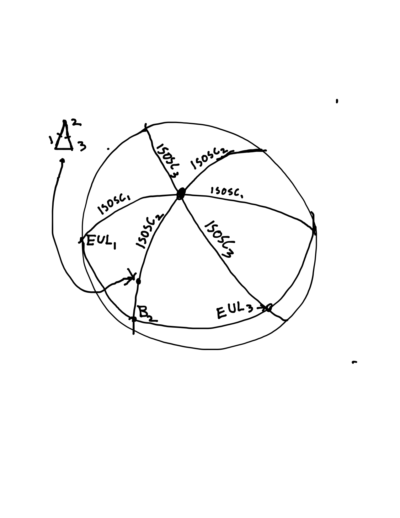
Figure 8. The shape sphere with the Isosceles great circles marked.

Label these circles $ISOSC_{1},ISOSC_{2},ISOSC_{3}$ according to the mass which forms the isosceles triangle’s vertex. For example $ISOSC_{1}$ is the circle consisting of those triangles for which $r_{12}=r_{13}$. Each circle $ISOSC_{i}$ intersects the collinear plane $w_{3}=0$ in two points, an Euler point $EUL_{i}$ which represents the configuration of Euler’s solution, and a binary collision point $B_{i}$ (our old ${\bf b}_{jk}$). For example $EUL_{1}\in ISOSC_{1}$ represents those degenerate triangles for which mass 1 lies at the midpoint of the segment formed by masses 2 and 3. Considered in shape space, the circle $ISOSC_{i}$ becomes a plane $\Pi_{i}$ and $EUL_{i}$ and $B_{i}$ becomes a ray lying in that plane.

We consider the problem of minimizing the shape space action $\int_{c}L_{shape}dt$ among all paths connecting $EUL_{1}$ to $ISOSC_{2}$ in a fixed time $T$. The difficult part of the proof is showing that this minimimum $\gamma_{*}$ actually exists and is collision-free. Once established, we know by the first variation orthogonality that $\gamma_{*}$ must hit the Euler ray $EUL_{1}$ orthogonally, and the isosceles plane $ISOSC_{2}$ orthogonality. This orthogonality allows us to continue the solution arc $\gamma_{*}$ by reflection. The equal mass condition insures that these reflections take solutions to solutions.

For example, the fact that $m_{1}=m_{3}$ implies that permutation of masses 1 and 3 is a linear isometric involution $\sigma_{2}:(q_{1},q_{2},q_{3})\mapsto(q_{3},q_{2},q_{1})$ of $\mathbb{C}^{3}$ (isometric relative to the mass metric) which preserves the potential and hence maps solutions to Newton’s equations to solutions to Newton’s equations. The effect of $\sigma_{2}$ on the shape sphere is a half-twist about the line connecting $EUL_{2}$ and $B_{2}$. If we compose $\sigma_{2}$ with the operation of reflection about the symmetry axis of isosceles triangle $\gamma_{*}(T)$ we obtain an action-preserving isometric involution $R_{2}$ whose the effect on shape space is that of reflection about the plane $ISOSC_{2}$. Thus $R_{2}(\gamma_{*})$ is a solution arc which connects $ISOSC_{2}$ to $EUL_{3}$ and whose derivative matches up with $\gamma_{*}$. It therefore agrees with the continuation of the solution $\gamma_{*}$, up to a time translation. We now have a solution on the interval $[0,2T]$ joining $EUL_{1}$ to $EUL_{3}$. Apply the half-twist $\sigma_{3}$ about the line connecting $EUL_{3}$ and $B_{3}$ to this continued solution to obtain a solution arc on the interval $[0,4T]$ connecting $EUL_{1}$ to $EUL_{2}$, and crossing $ISOSC_{2},EUL_{3},ISOSC_{1}$ in that order along the way. Continue to march around the sphere, applying half-twists or reflections as needed I obtain twelve solution arcs each congruent to the original arc $\gamma_{*}$ and whose derivatives all match up. The result is a smooth solution to the three-body equation which is periodic in shape space with period $12T$. With some extra work, we can show that the solution is actually periodic of period $12T$ in the original inertial space – i.e the plane, and that this curve $\gamma$ is a choreograpy. The curve $\gamma$ is the figure eight solution.

Definition 9.

An N-body choreography of period $T$ is a solution to N-body problem which has the particula form ${\bf q}(t)=(q_{1}(t),q_{2}(t),\ldots,q_{N}(t))$ where $q_{i}(t)=s(t-iT/N)$, $i=2,3,\ldots,N$ for some fixed $T$ periodic curve $s(t)$ in the plane (or space).

This curve is the figure eight, viewed in shape space. See figure 9.

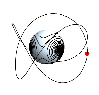
Figure 9. The figure eight as it appears in shape space.

History. The figure eight solution curve was discovered in 1994 using the principle of least action by C. Moore [9]. Chenciner and myself rediscovered the solution using the shape space least action principle in 2000. Our methods yielded a rigorous existence proof.

15. Summary

The perspective of shape space reduces many features of the Newtonian three-body problem to an investigation of curves on the shape sphere or even the shape space. These spaces have dimension 2 and 3 compared to the 12 dimensions of the original planar three-body phase space: 6 for the vertices of the moving triangle and 6 for their velocities. Our minds are not nearly as well attuned to 12 dimensional visualization as they are to 3 dimensional visualization. The reduction from 12 to 3 allows us hope of accurately and successfully applying the creative powers of our geometric visualization to better understand the three-body problem.

16. Acknowledgements.

I would like to thank Alain Chenciner, Alain Albouy, Carles Simo and Rick Moeckel for many conversations over the years. I would particularly like to Piet Hut for the use of figure 2 and Rick Moeckel for the use of figure 9.

References

- [1] V.I. Arnol’d, Mathematical Methods in Celestial Mechanics, 2nd ed. 1978, transl by A. Weinstein and K. Vogtman, Springer.
- [2] A. Chenciner [1997] A l’infini en temps fini, Séminaire Bourbaki, exp. 832, pp. 323-353, esp. p.331.
- [3] A. Chenciner and R. Montgomery, A remarkable periodic solution of the three-body problem in the case of equal masses, with Alain Chenciner, Annals of Mathematics, 152, 881-901 2000.
- [4] T. Fujiwara, H. Fukuda, A. Kameyama, H. Ozaki and M.Yamada [2004], Synchronised Similar Triangles, J. Phys. A: Math. Gen. 37 (2004) 10571-10584
- [5] L. Euler [1765] ; [1770], Considérations sur le problème de trois corps. Mémoires de l’Académie de Sciences de Berlin, vol. 19, pp. 194-220.
- [6] M. Herman [1998], Some open problems in dynamical systems, Proceedings of the International Congress of Mathematicians, Documenta Mathematica J. DMV, Extra volume ICM II, pp. 797–808
- [7] J-L. Lagrange [1772], Essai sur le Probléme des Trois Corps. Prix de l’Académie Royale des Sciences de Paris, tome IX, in volume 6 of œuvres (page 292).
- [8] R. Montgomery, Infinitely many syzygies, Arch. Rat. Mech.., 164, 4 (2002) 311–340.
- [9] C. Moore [1993] , Braids in Classical Gravity, Phys Rev Lett. v. 70, pp. 3675 3679.
- [10] I. Newton [1667], Philosophi Naturalis Principia Mathematica available at various sites on the web, including: http://en.wikisource.org/wiki/The_Mathematical_Principles_of_Natural_Philosophy_%281846%29
- [11] R. Feynman, R. Leighton, M. Sands, [1963], The Feynman Lectures on Physics v. 1 , Addison-Wesley Pub. Co.
- [12] D. Saari, [1984], The manifold structure for collision and hyperbolic-parabolic orbits in the n-body problem J.Diff. Eq. 55, 300-329.