IFT-UAM/CSIC-14-003

FTUAM-14-3

Exploring the role of the charm quark in the $\Delta I=1/2$ rule

E. Endress^a and C. Pena^a,b

^a Instituto de Física Teórica UAM/CSIC

c/Nicolás Cabrera 13-15, Universidad Autónoma de Madrid

Cantoblanco E-28049 Madrid, Spain

^b Departamento de Física Teórica, Universidad Autónoma de Madrid

Cantoblanco E-28049 Madrid, Spain

Abstract: We study the dependence on the charm quark mass of the leading-order low-energy constants of the $\Delta S=1$ effective Hamiltonian, with the aim of elucidating the role of the charm mass scale in the $\Delta I=1/2$ rule for $K\to\pi\pi$ decay. To that purpose, finite-volume Chiral Perturbation Theory predictions are matched to QCD simulations, performed in the quenched approximation with overlap fermions and $m_{u}=m_{d}=m_{s}$. Light quark masses range between a few MeV up to around one third of the physical strange mass, while charm masses range between $m_{u}$ and a few hundred MeV. Novel variance reduction techniques are used to obtain a signal for penguin contractions in correlation functions involving four-fermion operators. The important role played by the subtractions required to construct renormalised amplitudes for $m_{c}\neq m_{u}$ is discussed in detail. We find evidence that the moderate enhancement of the $\Delta I=1/2$ amplitude previously found in the GIM limit $m_{c}=m_{u}$ increases only slightly as $m_{c}$ abandons the light quark regime. Hints of a stronger enhancement for even higher values of $m_{c}$ are also found, but their confirmation requires a better understanding of the subtraction terms.

1 Introduction

The quantitative understanding of non-leptonic kaon decays, such as $K\to\pi\pi$, remains an elusive problem after several decades of study. Thus, no fully solid Standard Model computation of the value of $\epsilon^{\prime}/\epsilon$, or of the amplitudes involved in the famous $\Delta I=1/2$ rule, is available. In this paper we focus on the latter problem. The decay of a neutral kaon into a pair of pions with total isospin $I$ has an associated transition amplitude

$$T[K\to(\pi\pi)_{I}]=iA_{I}e^{i\delta_{I}}\,,$$ (1.1)

where $\delta_{I}$ is the pion scattering phase shift. Experiment finds that the amplitude in the $I=0$ channel is significantly larger than the one in the $I=2$ channel,

$$\frac{|A_{0}|}{|A_{2}|}\simeq 22.1\,.$$ (1.2)

Early analysis of the $\Delta I=1/2$ problem showed that, if its explanation is to be found in the Standard Model, the bulk of the enhancement must come from long-distance contributions generated by the strong interaction [1, 2]. Reliable determinations of the latter inevitably require a non-perturbative computation [3, 4].

The lattice regularisation of QCD is the only known approach capable of providing fully first-principles results at the non-perturbative level. Yet, lattice studies of $K\to\pi\pi$ have to face significant difficulties:

• The computation of transition amplitudes for two-body decays from the Euclidean correlation functions provided by lattice QCD requires non-trivial kinematical setups [7, 8, 9], which ultimately has a significant impact on the computational cost.

• The renormalisation of the relevant weak effective Hamiltonian $H_{\rm w}$ is complex. When the charm quark is not kept as an active degree of freedom the four-quark operators in $H_{\rm w}$ are power-divergent, and non-perturbative subtractions are needed to obtain finite amplitudes. Furthermore, even when the charm is not integrated out the same is true unless the regularisation preserves chiral symmetry. Thus, lattice studies with Wilson fermions are poised to deal with this problem. The use of lattice fermion regularisations with Ginsparg-Wilson fermions [12, 13, 14, 15, 16, 17, 18, 19, 20, 21], that possess an exact chiral symmetry and have been shown to preserve good renormalisation properties of the operators [22], is therefore advantageous. This, however, has again an impact on the computational cost, since Ginsparg-Wilson fermions are numerically expensive.

In recent years, computations that employ so-called domain wall fermions have succeeded in making significant progress in the study of non-leptonic kaon decays, by computing amplitudes involving the effective Hamiltonian without a charm quark [23, 24, 25, 26].

There are several possible sources for the $\Delta I=1/2$ enhancement within the context of strong interactions. This is ultimately connected to the presence of various scales in the problem: the charm quark mass scale $m_{c}\sim 1.3~{}{\rm GeV}$; the intrinsic QCD scale $\Lambda_{\rm QCD}\sim 250~{}{\rm MeV}$; and the scale $\lesssim 100~{}{\rm MeV}$ of pion final state interactions. In particular, the role of the charm quark and its associated mass scale as a possible cause for the $\Delta I=1/2$ enhancement was pointed out long ago [27]. However, charm effects are not easily apprehended when its contribution to $H_{\rm w}$ is integrated out. This, together with the much simpler renormalisation properties resulting from the presence of a working GIM mechanism, constitutes a strong case to keep the charm as an active degree of freedom in the low-energy treatment of electroweak effects.

In [28] a strategy was proposed to disentangle contributions from the various scales, and quantify them using numerical simulations. The starting point is the CP-conserving $\Delta S=1$ effective weak Hamiltonian with an active charm quark. One then constructs its counterpart within the low-energy effective description of QCD provided by Chiral Perturbation Theory (ChiPT). This is done for two different physical situations: the physical kinematics, where the charm is heavy and the relevant symmetry for the chiral dynamics is ${\rm SU}(3)_{\rm L}\times{\rm SU}(3)_{\rm R}$; and the unphysical GIM limit $m_{c}=m_{u}$, where the charm is light and the relevant chiral symmetry is ${\rm SU}(4)_{\rm L}\times{\rm SU}(4)_{\rm R}$. In either case, the low-energy constants (LECs) of the chiral effective Hamiltonian can be determined by matching suitable correlation functions in ChiPT and QCD. The use of the effective description, first proposed in [29], implies dealing with $K\to\pi$ transitions only, which has a double effect: it avoids the kinematical difficulties posed by the two-body decay, allowing for smaller volumes (and hence a reduced computational cost); and it neglects final-state interaction effects, which isolates one of the possible sources for enhancement. The calculation of the LECs corresponding to $\Delta I=1/2$ and $\Delta I=3/2$ transitions in the GIM limit will expose the effect from intrinsic QCD scales. The effect of a heavier charm quark can then be studied by monitoring the behaviour of the amplitudes as $m_{c}$ increases towards its physical value, exiting the domain of validity of ChiPT for the charm sector in the process.

Results in the GIM limit were obtained in [30, 31] from quenched QCD simulations with overlap quarks. It was found that in this case the $I=2$ amplitude is already very close to its physical value, and that a significant enhancement is already present. The $I=0$ amplitude is however still smaller than its physical value by roughly a factor of 4. The question is then left whether increasing $m_{c}$ towards heavy values provides the bulk of the missing enhancement. Extending the study to $m_{c}\gg m_{u}$ is however non-trivial, because it requires the computation of new correlation functions — in the form of so-called “penguin contractions” or “eye diagrams” — notoriously affected by severe signal-to-noise problems. The construction of renormalised amplitudes for $m_{c}\neq m_{u}$ also requires subtractions that eliminate logarithmic divergences not present in the GIM limit, which adds an extra layer of complication.

In this work we present the first results of an exploration of the effect of a heavier charm quark on the $\Delta I=1/2$ amplitude, extending the study in [30]. We will focus on the physics discussion and results; the variance reduction techniques developed for the computation are described in a companion paper [32]. Simulations will still be carried out in the quenched approximation. This is not expected to have a major impact on the qualitative results of the analysis, and avoids the large increase of the computational cost that dynamical overlap simulations would imply — or, alternatively, the technical and conceptual complications associated to a mixed-action strategy, in case one would like to use dynamical configurations obtained with a different fermion regularisation.

The layout of the paper is as follows. In Section 2 we summarise the strategy introduced in [28]. In Section 3 we discuss the role of subtraction terms, and how they can be treated. In Section 4 we discuss our lattice results for the relevant QCD correlation functions. In Section 5 these results are matched to ChiPT to extract the values of the leading-order LECs. Finally, Section 6 presents our conclusions and outlook. A number of technicalities are discussed in appendices.

2 Setup and strategy

The setup we follow to disentangle the role of the charm quark in the $\Delta I=1/2$ rule has been laid out in [28]. Here we summarise it, and refer the reader to that paper for a fully detailed discussion of the various aspects.

2.1 Effective weak Hamiltonian with an active charm quark

When the charm quark is kept as an active degree of freedom, and after neglecting the contribution from top quark loops, the effective Hamiltonian that describes $K\to\pi\pi$ decays in the Standard Model at scales well below $M_{W}$ has the form

$$H_{\rm w}(x)=\frac{g_{\rm w}^{2}}{4M_{W}^{2}}V_{us}^{*}V_{ud}\sum_{n}k_{n}Q_{n}(x)\,,$$ (2.3)

where $g_{\rm w}^{2}=4\sqrt{2}G_{\rm F}M_{W}^{2}$, the sum runs over all the composite operators $Q_{n}$ with engineering dimension $d\leq 6$ and appropriate transformation properties under the relevant symmetries, and $k_{n}$ are the corresponding Wilson coefficients.

The relevant global symmetry group is ${\rm SU}(4)_{\rm L}\times{\rm SU}(4)_{\rm R}$, and the left-handed character of electroweak interactions demands that operators are singlets under ${\rm SU}(4)_{\rm R}$. Only two four-quark operators with the correct flavour content and transformation properties can be constructed, namely

$$Q_{1}^{\pm}=J_{\mu}^{su}J_{\mu}^{ud}\pm J_{\mu}^{sd}J_{\mu}^{uu}~{}-~{}[u\leftrightarrow c]\,,$$ (2.4)

where $J_{\mu}$ is the left-handed current

$$J_{\mu}^{\alpha\beta}=(\bar{\psi}_{\alpha}\gamma_{\mu}P_{-}\psi_{\beta})\,,$$ (2.5)

$P_{\pm}={\scriptstyle{{1\over 2}}}(\mathbf{1}\pm\gamma_{5})$, and parentheses around quark bilinears indicate that they are traced over spin and colour. $Q_{1}^{+},Q_{1}^{-}$ transform in irreducible representations of ${\rm SU}(4)_{\rm L}$ of dimensions 84 and 20, respectively. The only two other possible operators are quark bilinears, multiplied by factors involving the quark mass matrix $M$; when the latter is diagonal, $M={\rm diag}(m_{u},m_{d},m_{s},m_{c})$, the two operators are actually identical, and reduce to

$$\begin{split}Q_{2}^{\pm}&=(m_{u}^{2}-m_{c}^{2})\left\{m_{d}(\bar{s}P_{+}d)\,+\,m_{s}(\bar{s}P_{-}d)\right\}\\ &={\scriptstyle{{1\over 2}}}(m_{u}^{2}-m_{c}^{2})\left\{(m_{d}+m_{s})(\bar{s}d)-(m_{s}-m_{d})(\bar{s}\gamma_{5}d)\right\}\,.\end{split}$$ (2.6)

We will keep the $\pm$ superscript in this operator nonetheless, for the sake of notational consistency. Note that the effective Hamiltonian in Eq. (2.3) is much simpler than the one obtained when the charm quark is integrated out — in that case, $H_{\rm w}$ will contain ten operators (of which some are redundant). The two main advantages of keeping an active charm are that the renormalisation properties of composite operators (see below) are much simpler due to the presence of a working GIM mechanism; and it is possible to study the dependence of QCD amplitudes on $m_{c}$ directly.

For the latter purpose, it turns out to be convenient to also have Eq. (2.3) rewritten in terms of operators that transform in irreducible representations of the flavour group ${\rm SU}(3)_{\rm L}\times{\rm SU}(3)_{\rm R}$ spanned by the light $u,d,s$ quarks. The outcome of this exercise is [33]

$$H_{\rm w}=\frac{g_{\rm w}^{2}}{4M_{W}^{2}}V_{us}^{*}V_{ud}\left\{k_{1}^{+}Q_{u}^{+}+\frac{k_{1}^{+}}{5}\,R^{+}+k_{1}^{-}R^{-}-k_{1}^{+}Q_{c}^{+}-k_{1}^{-}Q_{c}^{-}+k_{2}^{+}Q_{2}^{+}+k_{2}^{-}Q_{2}^{-}\right\}\,,$$ (2.7)

where

$$Q_{u}^{+} =J_{\mu}^{su}J_{\mu}^{ud}+J_{\mu}^{sd}J_{\mu}^{uu}-\frac{1}{5}\sum_{q=u,d,s}\left\{J_{\mu}^{sq}J_{\mu}^{qd}+J_{\mu}^{sd}J_{\mu}^{qq}\right\}\,,$$ (2.8)

$$R^{\pm} =\sum_{q=u,d,s}\left\{J_{\mu}^{sq}J_{\mu}^{qd}\pm J_{\mu}^{sd}J_{\mu}^{qq}\right\}\,,$$ (2.9)

$$Q_{c}^{\pm} =J_{\mu}^{sc}J_{\mu}^{cd}\pm J_{\mu}^{sd}J_{\mu}^{cc}\,.$$ (2.10)

The operator $Q_{u}^{+}$ transforms under the 27-plet of ${\rm SU}(3)_{\rm L}$, while all other operators transform under irreducible representations of dimension 8. Note the trivial identities $Q_{1}^{+}=Q_{u}^{+}+\frac{1}{5}R^{+}-Q_{c}^{+},~{}Q_{1}^{-}=R^{-}-Q_{c}^{-}$.

2.2 Renormalisation and mixing

The full weak Hamiltonian is finite, and does not require any renormalisation. The operators $Q_{1,2}^{\pm}$, on the other hand, must be renormalised. Assuming that the regularisation preserves enough of the relevant symmetries (which will be the case in what follows), the general relation between bare and renormalised (denoted with a bar) operators is

$$\begin{split}\bar{Q}_{1}^{\pm}&=Z_{11}^{\pm}Q_{1}^{\pm}+Z_{12}^{\pm}Q_{2}^{\pm}\,,\\ \bar{Q}_{2}^{\pm}&=Z_{21}^{\pm}Q_{1}^{\pm}+Z_{22}^{\pm}Q_{2}^{\pm}\,.\end{split}$$ (2.11)

Since the operator $Q_{2}^{\pm}$ only contains products of non-singlet chiral densities times linear combinations of quark masses, it is multiplicatively renormalisable, which allows to choose $Z_{21}^{\pm}=0$. Furthermore, as a consequence of the GIM mechanism the contribution of $Q_{2}^{\pm}$ to renormalised operators vanishes when $m_{u}=m_{c}$; this allows to fix $Z_{11}^{\pm}$ at vanishing quark masses. It is then enough to fix $Z_{12}^{\pm}$ such that any remaining divergences are subtracted. Equivalently, one can rewrite the effective Hamiltonian as

$$H_{\rm w}=\sum_{\sigma=\pm}k_{1}^{\sigma}(\mu)Z_{11}^{\sigma}(\mu)\left\{Q_{1}^{\sigma}\,+\,c^{\sigma}Q_{2}^{\sigma}\right\}\,,$$ (2.12)

where $Q_{i}^{\pm}$ are the bare operators, and impose two subtraction conditions that determine the coefficients $c^{\pm}$ in such a way that the only remaining divergence in the subtracted operators $Q_{1}^{\pm}\,+\,c^{\pm}Q_{2}^{\pm}$ are eliminated by $Z_{11}^{\pm}$. (This is obviously equivalent to fixing $Z_{12}^{\pm}$). This procedure will be discussed in detail below. Note that the operator mixing encoded in $c^{\pm}$ is a radiative effect, so one expects $c^{\pm}$ to be naturally of ${\cal O}(\alpha_{\rm s})$, leading to a suppression of the contribution of $Q_{2}^{\pm}$ to physical amplitudes. Note also that the coefficients $c^{\pm}$ are expected to contain logarithmic divergences, since the anomalous dimensions of the bare operators $Q_{1}^{\pm}$ and $Q_{2}^{\pm}$ are different. In a mass independent renormalisation scheme, one should isolate the values of $c^{\pm}$ in the chiral limit and compute them at the same scale at which the overall renormalisation constants $Z_{11}^{\pm}$ and the Wilson coefficients $k_{1}^{\pm}$ are computed.

Once the operators are renormalised, they have to be combined with Wilson coefficients into the weak Hamiltonian. Wilson coefficients can be computed from the perturbative anomalous dimensions, which are known at next-to-leading order in various dimensional regularisation-based schemes, as well as in the regularisation-independent (RI) scheme [34, 35, 36, 37]. Correlation functions involving the operators will be computed on the lattice, and are best non-perturbatively renormalised; the two schemes of choice to this purpose are RI and Schrödinger Functional (SF) schemes. The main difference between the two options is that the RI procedure allows to renormalise the operators at scales in the ballpark of few ${\rm GeV}$, while the SF method provides renormalisation constants at any value of the scale between $\mu\sim\Lambda_{\rm QCD}$ and $\mu\sim M_{W}$. The use of RI thus allows to compute the product $k_{n}(\mu)\bar{Q}_{n}(\mu)$ directly, with the disadvantage that the value of $\mu$ is relatively low and the uncertainty related to the perturbative truncation in $k_{n}$ has to be assessed. With SF, on the other hand, a matching between renormalisation schemes is needed, but it can be performed at high energy scales, where the convergence of perturbation theory is very good. This will thus be our method of choice.

A convenient way to embody this procedure is to work in a renormalisation group invariant (RGI) formulation. To that purpose one defines RGI operators and Wilson coefficients as

$$Q^{\rm\scriptscriptstyle RGI}=U(\mu/\Lambda)Q(\mu)=U(\mu/\Lambda)Z(\mu)Q\,,~{}~{}~{}~{}~{}~{}~{}k^{\rm\scriptscriptstyle RGI}=U(\mu/\Lambda)^{-1}k(\mu)\,,$$ (2.13)

where the RG running factor $U(\mu/\Lambda)$ that connects the renormalised quantity at scale $\mu$ to its RGI counterpart is given by

$$U(\mu/\Lambda)=\left[2b_{0}\kern 1.0pt\overline{\kern-1.0ptg\kern 0.0pt}\kern 1.0pt^{2}(\mu)\right]^{\frac{\gamma_{0}}{2b_{0}}}\exp\left\{-\int_{0}^{\kern 1.0pt\overline{\kern-1.0ptg\kern 0.0pt}\kern 1.0pt(\mu)}{\rm d}g\left[\frac{\gamma(g)}{\beta(g)}+\frac{\gamma_{0}}{b_{0}g}\right]\right\}\,,$$ (2.14)

where $\gamma$ and $\beta$ are the anomalous dimension of $Q$ and the RG $\beta$-function in the scheme of choice, respectively, and $\gamma_{0},b_{0}$ are the leading-order coefficients of their perturbative expansions. The use of the SF scheme allows to compute both $Z(\mu)$ and $U(\mu/\Lambda)$ for small values of $\mu/\Lambda$; in the case of the running factor this is achieved by splitting it as

$$U(\mu/\Lambda)=U(M_{W}/\Lambda)\,\frac{U(\mu/\Lambda)}{U(M_{W}/\Lambda)}\,,$$ (2.15)

where the second factor on the r.h.s. is computed non-perturbatively, and the first one is computed at next-to-leading order with a small perturbative truncation error of order $\alpha_{s}(M_{W})^{3}\sim{\cal O}(10^{-3})$. The RGI Wilson coefficient can instead be computed directly as $k^{\rm\scriptscriptstyle RGI}=U(M_{W}/\Lambda)^{-1}k(M_{W})$, with the same degree of perturbative uncertainty. In view of the construction of the weak Hamiltonian, it is convenient to define the quantities

$${\cal Z}_{1}^{\pm}\equiv k_{1}^{\pm;{\rm RGI}}U_{1}^{\pm}(\mu/\Lambda)\frac{Z_{11}^{\pm}(\mu)}{Z_{\rm\scriptscriptstyle A}^{2}}\,,$$ (2.16)

where $Z_{\rm\scriptscriptstyle A}$ is the normalisation factor of the left-handed current (which will be non-trivial in the lattice regularisation of QCD that we will introduced later). Note that ${\cal Z}_{1}^{\pm}$ is independent by construction of the renormalisation scale $\mu$.

The running factor $U(\mu/\Lambda)$ has been computed non-perturbatively in [38, 39] with $N_{\mathrm{\scriptstyle f}}=0$ and $N_{\mathrm{\scriptstyle f}}=2$ dynamical flavours, respectively. The renormalisation factors $Z_{11}^{\pm}(\mu)/Z_{\rm\scriptscriptstyle A}^{2}$ for the overlap fermion regularisation that we will employ in this work have been determined in quenched QCD in [40].

2.3 Effective low-energy description in Chiral Perturbation Theory

As discussed in the introduction, a direct computation of $K\to\pi\pi$ amplitudes, requiring large physical volumes, is beyond the current scope of our work. We thus resort to computing instead the LECs in the ChiPT counterpart of the effective weak Hamiltonian, from which the amplitudes can be computed at some given order in the chiral expansion. Since our main emphasis is to understand their dependence on $m_{c}$, we will face two different physical situations: the strict GIM limit, where all quark masses are light and degenerate; and the “physical” kinematics, where $m_{u}=m_{d}=m_{s}$ are kept light and $m_{c}\gg m_{u}$. In the former case, all four quarks can be treated within ChiPT, while in the latter only the light flavours enter the effective description; therefore, two different versions of the chiral effective Hamiltonian will be needed, with ${\rm SU}(4)$ and ${\rm SU}(3)$ symmetries, respectively.

The construction of the relevant chiral effective weak Hamiltonians has been reviewed in [33]. Given a leading-order chiral Lagrangian of the form (either for $U\in{\rm SU}(N_{\mathrm{\scriptstyle f}}=4)$ or $U\in{\rm SU}(N_{\mathrm{\scriptstyle f}}=3)$)

$${\cal L}=\frac{F^{2}}{4}{\rm Tr}\left[(\partial_{\mu}U)\partial_{\mu}U^{\dagger}\right]-\frac{\Sigma}{2}{\rm Tr}\left[UM^{\dagger}e^{i\theta/N_{\mathrm{\scriptstyle f}}}+MU^{\dagger}e^{-i\theta/N_{\mathrm{\scriptstyle f}}}\right]\,,$$ (2.17)

where $M$ is the mass matrix and $\theta$ the vacuum angle, the leading-order ${\rm SU}(4)$ Hamiltonian reads

$${\cal H}_{\rm w}^{(4)}=\frac{g_{\rm w}^{2}}{4M_{W}^{2}}V_{us}^{*}V_{ud}\sum_{\sigma=\pm}\left\{g_{1}^{\sigma}{\cal Q}_{1}^{\sigma}\,+\,g_{2}^{\sigma}{\cal Q}_{2}^{\sigma}\right\}\,,$$ (2.18)

where $g_{1,2}^{\pm}$ are LECs,

$${\cal Q}_{1}^{\pm}={\cal J}_{\mu}^{su}{\cal J}_{\mu}^{ud}\pm{\cal J}_{\mu}^{sd}{\cal J}_{\mu}^{uu}\,-\,[u\leftrightarrow c]\,,$$ (2.19)

${\cal J}_{\mu}$ is the left-handed chiral current

$${\cal J}_{\mu}=\frac{F^{2}}{\sqrt{2}}\,U\partial_{\mu}U^{\dagger}\,,$$ (2.20)

and superscripts indicate matrix components in flavour space. The ${\rm SU}(3)$ Hamiltonian has instead the form

$${\cal H}_{\rm w}^{(3)}=\frac{g_{\rm w}^{2}}{4M_{W}^{2}}V_{us}^{*}V_{ud}\left\{g_{27}{\cal Q}_{27}\,+\,g_{8}{\cal Q}_{8}\,+\,g^{\prime}_{8}{\cal Q}^{\prime}_{8}\right\}\,,$$ (2.21)

where

$${\cal Q}_{27} =\frac{2}{5}\,{\cal J}_{\mu}^{su}{\cal J}_{\mu}^{ud}+\frac{3}{5}\,{\cal J}_{\mu}^{sd}{\cal J}_{\mu}^{uu}\,,$$ (2.22)

$${\cal Q}_{8} =\frac{1}{2}\sum_{q=u,d,s}{\cal J}_{\mu}^{sq}{\cal J}_{\mu}^{qd}\,,$$ (2.23)

$${\cal Q}^{\prime}_{8} =m_{l}\Sigma F^{2}\left[Ue^{i\theta/N_{\mathrm{\scriptstyle f}}}+U^{\dagger}e^{-i\theta/N_{f}}\right]^{sd}\,,$$ (2.24)

where $m_{l}\equiv m_{u}=m_{d}=m_{s}$. Indeed, in order to avoid unessential complications related to the soft breaking of the ${\rm SU}(3)$ vector symmetry, we will always work in the limit of degenerate up, down, and strange masses, which will be assumed hereafter.

LECs will be determined by matching QCD correlation functions containing the weak Hamiltonian with ChiPT correlation functions containing its chiral counterpart. Matching conditions can be imposed separately in different symmetry sectors, by identifying sets of operators on both sides that transform in the same way under the relevant chiral symmetry. In the case of the matching to ${\rm SU}(4)$ ChiPT this is straightforward: ${\cal Q}_{1,2}^{\pm}$ and $Q_{1,2}^{\pm}$ have exactly the same transformation properties under ${\rm SU}(4)_{\rm L}$. In the case of ${\rm SU}(3)$ ChiPT, on the other hand, one finds that ${\cal Q}_{27}$ transforms in the 27-plet of ${\rm SU}(3)_{\rm L}$, while ${\cal Q}_{8}$ and ${\cal Q}^{\prime}_{8}$ transforms as octets; since on the QCD side there are one 27-plet and several octet operators, the matching will be somewhat more involved. Furthermore, as is well-known, $K\to\pi\pi$ amplitudes depend on $g_{27}$ and $g_{8}$ but not on $g^{\prime}_{8}$ [29, 41], rendering the latter essentially arbitrary; as a matter of fact, the appearance of $g^{\prime}_{8}$ reflects the need for subtractions in QCD amplitudes, as will be discussed in greater detail below.

Note that, since the charm quark is always kept as an active degree of freedom in QCD, this will imply that the ${\rm SU}(3)$ LECs $g_{27},g_{8}$ will be functions of $m_{c}$. One can actually consider the matching of the chiral Hamiltonians ${\cal H}_{\rm w}^{(4)}$ and ${\cal H}_{\rm w}^{(3)}$ in a regime where $m_{c}>m_{u}=m_{d}=m_{s}$ but such that the charm can still be treated within ChiPT, from which point of view charmed mesons behave as decoupling particles. This has been studied in [42], where explicit expressions for $g_{27}(m_{c}),g_{8}(m_{c})$ in terms of LO and (unknown) next-to-leading order LECs in ${\rm SU}(4)$ ChiPT are provided. The leading-order matching reads

$$g_{27}(0)=g_{1}^{+}\,,~{}~{}~{}~{}~{}~{}~{}~{}~{}~{}~{}~{}~{}~{}~{}g_{8}(0)=g_{1}^{-}\,+\,\frac{1}{5}\,g_{1}^{+}\,.$$ (2.25)

On the other hand, one can take the leading-order results for $|A_{0}|$ and $|A_{2}|$ in ${\rm SU}(3)$ ChiPT and match them to the experimental values of the amplitudes, interpreting the result as a phenomenological determination of the LECs at the physical value $\overline{m}_{c}$ of the charm quark mass. The result of this exercise is

$$|g_{27}^{\rm exp}(\overline{m}_{c})|\sim 0.50\,,~{}~{}~{}~{}~{}~{}~{}~{}~{}~{}~{}~{}~{}~{}~{}|g_{8}^{\rm exp}(\overline{m}_{c})|\sim 10.5\,.$$ (2.26)

One important ingredient of our setup is that we work both in the standard, $p$-regime of ChiPT, and in the so-called $\epsilon$-regime [43, 44] (see also [45, 46]). Here $p$-regime means working in large volumes measured in terms of the pion Compton wavelength, i.e. $m_{\pi}L\gg 1$ if a four-dimensional box of dimensions $L^{3}\times T$ is considered; $\epsilon$-regime means keeping a large volume (i.e. the implicit $F_{\pi}L\gg 1$ prerrequisite for the chiral expansion to work is fulfilled) but working at very small quark masses, such that the “pion” Compton wavelength is of the order of $L$ — or, more precisely, $m\Sigma V\lesssim 1$, where $m$ is the light quark mass, $\Sigma$ is the chiral condensate, and $V$ is the four-dimensional volume. Furthermore, one should keep $T\sim L$, since at $T/L\gg 1$ a different kinematical region — the $\delta$-regime [47] — arises. The main advantage of considering the $\epsilon$-regime instead of the physical $p$-regime is that mass effects are suppressed in the former, and the chiral expansion is rearranged such that less operators appear at any given order in the expansion with respect to the $p$-regime [48]. This allows for potentially cleaner determinations of the leading-order LECs — especially so in the case of effective Hamiltonians for non-leptonic meson decay, which display a large number of new terms at NLO in the chiral expansion [49]. On the other hand, finite-volume effects are obviously large in the $\epsilon$-regime, being typically polynomial and not exponentially suppressed as in the $p$-regime. Finally, out of technical convenience correlation functions in the $\epsilon$-regime are computed at a fixed value of the topological charge.

It can be shown [43] that LECs are universal, in the sense that the same values are obtained when ChiPT is matched to QCD in either kinematical regime. Since the systematic uncertainties induced by the truncation of the chiral expansion are however different in each case, being able to perform consistent matching in both regimes implies a much higher degree of control on the final results. In particular, the ChiPT correlation functions involved in the matching for leading-order LECs in the chiral effective Hamiltonian will not depend on extra LECs up to NNLO corrections — NLO contributions are purely finite-volume effects, which are exactly calculable. Note that on the QCD side, the need of having non-perturbative results at very low quark masses and for a well-defined value of the topological charge in order to work in the $\epsilon$-regime implies that lattice regularisations with exact chiral symmetry are strongly preferred.

One final comment concerns the use of quenched Chiral Perturbation Theory (qChiPT) to describe quenched QCD data. As is well-known, qChiPT displays unphysical artifacts; in particular, in the context of $K\to\pi\pi$ transitions Golterman-Pallante ambiguities make the matching of QCD to ${\rm SU}(3)$ qChiPT ill-defined [50, 51]. This is however not the case for ${\rm SU}(4)$, where the ratios of correlation functions we will deal with (see below) present no ambiguities in the quenched approximation, as discussed in [28, 33]. Quenched results are not worked out explicitly in [33] for ${\rm SU}(3)$ ChiPT. As can be seen in the formulae gathered in Appendix A, while the $\epsilon$-regime formulae are essentially insensitive to quenching, the NLO prediction $p$-regime predictions for the relevant correlation functions in the octet channel displays $1/N_{\rm f}$ factors, that signal the need to take into account non-decoupled singlet contributions to repeat the computation in the quenched case. Here we will take the unquenched formulae as an operational description, and perform fits with various values of $N_{\rm f}$ (and hence different coefficients in the chiral logs) to check the dependence of the LECs on the value of $N_{\rm f}$, and adscribe a systematic uncertainty to fit results (see Section 5 for details).

2.4 Matching ChiPT to QCD

2.4.1 $m_{c}=m_{l}$

When all quarks are light and degenerate the effective low-energy description of $\Delta S=1$ processes is given by Eq. (2.18). Contributions from $Q_{2}^{\pm}$ (in QCD) and ${\cal Q}_{2}^{\pm}$ (in ChiPT) drop because they are proportional to $m_{u}-m_{c}$; one is thus left with the problem of determining the LECs $g_{1}^{\pm}$. As explained above, the correspondence between QCD and ChiPT operators in this case is straightforward. The matching can be easily performed using three-point functions of the operators in the effective Hamiltonian with quark bilinears such that flavour indices are saturated. A technically convenient choice for the latter is to employ left-handed currents, leading to the correlation functions

$$C_{i}^{\pm}(x_{0},y_{0}) =\int{\rm d}^{3}x\int{\rm d}^{3}y\,\langle J_{0}^{du}(x)\,Q_{i}^{\pm}(0)\,J_{0}^{us}(y)\rangle\,,$$ (2.27)

$$C(x_{0}) =\int{\rm d}^{3}x\,\langle J_{0}^{\alpha\beta}(x)\,J_{0}^{\beta\alpha}(0)\rangle\,,$$ (2.28)

where $\alpha,\beta$ are distinct light flavour indices (not summed over). The ratios

$$R_{i}^{\pm}(x_{0},y_{0})=\frac{C_{i}^{\pm}(x_{0},y_{0})}{C(x_{0})C(y_{0})}\,,$$ (2.29)

will then be proportional to the matrix elements $\langle\pi|Q_{1}^{\pm}|K\rangle$ (with mass-degenerate kaon and pion) when $x_{0}\to+\infty,y_{0}\to-\infty$. The equivalent ChiPT quantities are

$${\cal C}(x_{0}) =\int{\rm d}^{3}x\,\langle{\cal J}_{0}^{ud}(x)\,{\cal J}_{0}^{du}(0)\rangle_{{\rm SU}(4)}\,,$$ (2.30)

$${\cal C}_{i}^{\pm}(x_{0},y_{0}) =\int{\rm d}^{3}x\int{\rm d}^{3}y\,\langle{\cal J}_{0}^{du}(x)\,{\cal Q}_{i}^{\pm}(0)\,{\cal J}_{0}^{us}(y)\rangle_{{\rm SU}(4)}\,,$$ (2.31)

$${\cal R}_{i}^{\pm}(x_{0},y_{0}) =\frac{{\cal C}_{i}^{\pm}(x_{0},y_{0})}{{\cal C}(x_{0}){\cal C}(y_{0})}\,,$$ (2.32)

where the notation $\langle\rangle_{{\rm SU}(4)}$ emphasises the use of the appropriate effective theory. The LECs in the chiral weak Hamiltonian can then be readily extracted from the matching condition

$${\cal Z}_{1}^{\pm}R_{1}^{\pm}(x_{0},y_{0})=g_{1}^{\pm}{\cal R}_{1}^{\pm}(x_{0},y_{0})\,.$$ (2.33)

Formulae for ChiPT quantities are given in Appendix A.

2.4.2 $m_{c}\gg m_{l}$

A similar strategy to the one just described can be pursued to match QCD with $m_{c}\gg m_{l}$ to ${\rm SU}(3)$ ChiPT. One first defines new three-point functions in both QCD

$$C_{u}^{+}(x_{0},y_{0})=\int{\rm d}^{3}x\int{\rm d}^{3}y\,\langle J_{0}^{du}(x)\,Q_{u}^{+}(0)\,J_{0}^{us}(y)\rangle\,,$$ (2.34)

and ChiPT

$${\cal C}_{27}(x_{0},y_{0}) =\int{\rm d}^{3}x\int{\rm d}^{3}y\,\langle{\cal J}_{0}^{du}(x)\,{\cal Q}_{27}(0)\,{\cal J}_{0}^{us}(y)\rangle_{{\rm SU}(3)}\,,$$ (2.35)

$${\cal C}_{8}(x_{0},y_{0}) =\int{\rm d}^{3}x\int{\rm d}^{3}y\,\langle{\cal J}_{0}^{du}(x)\,{\cal Q}_{8}(0)\,{\cal J}_{0}^{us}(y)\rangle_{{\rm SU}(3)}\,,$$ (2.36)

$${\cal C}^{\prime}_{8}(x_{0},y_{0}) =\int{\rm d}^{3}x\int{\rm d}^{3}y\,\langle{\cal J}_{0}^{du}(x)\,{\cal Q}^{\prime}_{8}(0)\,{\cal J}_{0}^{us}(y)\rangle_{{\rm SU}(3)}\,,$$ (2.37)

and the corresponding ratios $R_{u}^{+},{\cal R}_{27},{\cal R}_{8},{\cal R}^{\prime}_{8}$ by dividing them with products of current two-point functions. Next one can impose matching conditions in both the 27-plet and octet channels,

$$R_{27}(x_{0},y_{0}) =g_{27}{\cal R}_{27}(x_{0},y_{0})\,,$$ (2.38)

$$R_{8}(x_{0},y_{0}) =g_{8}{\cal R}_{8}(x_{0},y_{0})+g^{\prime}_{8}{\cal R}^{\prime}_{8}(x_{0},y_{0})\,,$$ (2.39)

where

$$R_{27} ={\cal Z}_{1}^{+}R_{u}^{+}\,,$$ (2.40)

$$R_{8} ={\cal Z}_{1}^{+}\left[R_{1}^{+}-R_{u}^{+}+c^{+}R_{2}^{+}\right]+{\cal Z}_{1}^{-}\left[R_{1}^{-}+c^{-}R_{2}^{-}\right]\,.$$ (2.41)

Note that there is no contribution from the pure-octet correlator $R_{2}^{+}$ in the 27-plet channel.

It has to be stressed that the matching conditions in Eqs. (2.38,2.39) immediately imply that the LECs acquire a dependence on $m_{c}$. Furthermore, the matching condition Eq. (2.39) provides, in principle, only a linear combination of the two octet LECs; in particular, it does not directly allow to disentangle the physical ChiPT octet contribution with $g_{8}$ from the unphysical one with $g^{\prime}_{8}$. As will shown below, however, typical conditions to determine the subtraction coefficients $c^{\pm}$ required to construct renormalised QCD amplitudes simultaneously fix the value of $g^{\prime}_{8}$, which is then no longer an unknown. Eq. (2.39) does then allow to determine $g_{8}$ unambiguously. Formulae for ChiPT quantities are again provided in Appendix A.

2.5 Results in the GIM limit and scope of the present work

The ${\rm SU}(4)$ LECs $g_{1}^{\pm}$ were determined in [30] by computing the renormalised ratios of correlation functions ${\cal Z}_{1}^{\pm}R_{1}^{\pm}$ in lattice QCD in the quenched approximation at fixed volume and lattice spacing and keeping $m_{c}=m_{l}$. Computations were performed at four $p$-regime and one $\epsilon$-regime values of $m_{l}$; renormalisation factors were separately determined in [40]. The results were found

$$g_{1}^{+}=0.51(9)\,,~{}~{}~{}~{}~{}~{}~{}~{}~{}g_{1}^{-}=2.6(5)\,,$$ (2.42)

leading via Eq. (2.25) to

$$g_{27}(0)=0.51(9)\,,~{}~{}~{}~{}~{}~{}~{}~{}~{}g_{8}(0)=2.7(5)\,,$$ (2.43)

that can be compared with the phenomenological expectation in Eq. (2.26). It can then be concluded that

1. The approximations involved in the above computation provide the correct value for the $\Delta I=3/2$ amplitudes parametrised by $g_{27}$ (which are indeed expected to have little sensitivity to the value of $m_{c}$).

2. Pure low-energy QCD effects, combined with the well-known short-distance contribution given by the ratio of Wilson coefficients $k_{1}^{-}/k_{1}^{+}$, are responsible for a significant enhancement of the decay amplitude in the $\Delta I=1/2$ channel. The latter is however still a factor $\sim 4$ smaller than the phenomenological value.

Therefore, barring (unlikely) large cutoff effects in the $m_{c}=m_{l}$ lattice QCD computation, as well as the possibility of large quenching artifacts, an explanation of the $\Delta I=1/2$ rule that is purely based on Standard Model physics requires either a significant increase in $g_{8}(m_{c})$ when $m_{c}\gg m_{l}$; a strong effect due to pion rescattering in physical $K\to\pi\pi$ decays; or a combination of the two. The aim of the present work is to explore the dependence of $g_{8}$ on $m_{c}$, by extending the study of [40] to the case $m_{c}\neq m_{l}$. As we will discuss, a major technical challenge for this is the computation of the new contributions to amplitudes involving the four-fermion operators $Q_{1}^{\pm}$ that arise outside the $m_{c}=m_{u}$ limit.

3 The role of the subtraction term

As discussed above, outside the GIM limit $m_{u}=m_{c}$, and for our kinematics $m_{u}=m_{d}=m_{s}=m_{l}$, the renormalised matrix elements $\langle\pi(\mathbf{p}=\mathbf{0})|\bar{Q}_{1}^{\pm}|K(\mathbf{p}=\mathbf{0})\rangle$ are a linear combination of the bare $\langle\pi|Q_{1}^{\pm}|K\rangle$ matrix elements and the subtraction term $\langle\pi|Q_{2}^{\pm}|K\rangle$, cf. Eq. (2.12). In this section we will discuss the contribution of the subtraction term, as well as two possible procedures to determine the subtraction coefficients $c^{\pm}$: fixing $c^{\pm}$ by prescribing arbitrary values for the unphysical renormalised amplitudes $\langle 0|\bar{Q}_{1}^{\pm}|K\rangle$; and a variant of this method that involves two-point functions of $\bar{Q}_{1}^{\pm}$ in the $\epsilon$-regime. We will also discuss the behaviour of the subtraction coefficients in perturbation theory.

3.1 Matrix elements of $Q_{2}^{\pm}$

It is first of all interesting to note that the properties of amplitudes involving $Q_{2}^{\pm}$ are considerably simplified if, as will be the case in what follows, one is only interested in matrix elements of the effective weak Hamiltonian with no momentum transfer between the initial and final state. Using chiral Ward-Takahashi identities, the contribution from the operators $(\bar{s}P_{\pm}d)$ contained in $Q_{2}^{\pm}$ to any amplitude can be rewritten as

$$\langle f|(\bar{s}P_{\pm}d)|i\rangle=\frac{\langle f|\partial_{\mu}(\bar{s}\gamma_{\mu}d)|i\rangle}{m_{s}-m_{d}}\,\pm\,\frac{\langle f|\partial_{\mu}(\bar{s}\gamma_{\mu}\gamma_{5}d)|i\rangle}{m_{s}+m_{d}}\,.$$ (3.44)

When $m_{s}\neq m_{d}$, this immediately implies that the matrix element is proportional to the four-momentum transfer, and vanishes if the latter is zero. When $m_{s}=m_{d}$, on the other hand, the first term on the r.h.s. has vanishing numerator and denominator, and the quark mass dependence of $\langle f|\partial_{\mu}(\bar{s}\gamma_{\mu}d)|i\rangle$ has to be studied in order to find the value of the ratio in the limit $m_{s}\to m_{d}$.

In physical, $p$-regime kinematics, and for large Euclidean time separations between the operators, the QCD three-point functions involved in the matching to ChiPT are proportional to the transition amplitude $\langle\pi^{+}|H_{\rm w}|K^{+}\rangle$. Taking $|i\rangle=|K^{+}(p)\rangle,|f\rangle=|\pi^{+}(k)\rangle$ in Eq. (3.44), the contribution from the axial current term vanishes due to parity conservation, and the standard parametrisation of meson-meson matrix elements of the vector current in terms of vector ($f_{+}$) and scalar ($f_{0}$) form factors leads to

$$\begin{split}\langle\pi^{+}(k)|(\bar{s}d)|K^{+}(p)\rangle&=\frac{\langle\pi^{+}(k)|\partial_{\mu}(\bar{s}\gamma_{\mu}d)|K^{+}(p)\rangle}{m_{s}-m_{d}}\\ &=\frac{q_{\mu}\left[(p+k-\Delta)_{\mu}f_{+}(q^{2})+\Delta_{\mu}f_{0}(q^{2})\right]}{m_{s}-m_{d}}\,,\end{split}$$ (3.45)

where $q=p-k$, $\Delta_{\mu}=(m_{K}^{2}-m_{\pi}^{2})q_{\mu}/q^{2}$, and the normalisation convention $f_{+}(0)=f_{0}(0)$ applies. If the external states are on-shell, the above expression reduces to

$$\langle\pi^{+}(k)|(\bar{s}d)|K^{+}(p)\rangle=\frac{m_{K}^{2}-m_{\pi}^{2}}{m_{s}-m_{d}}\,f_{0}(q^{2})\,,$$ (3.46)

which does not vanish for $m_{s}\neq m_{d}$ (in which case the momentum transfer is indeed non-zero). If now we take our preferred kinematics $m_{u}=m_{d}=m_{s}$ we will have $m_{K}=m_{\pi}$, and the momentum transfer vanishes; but the matrix element is still non-zero, since the ratio $(m_{K}^{2}-m_{\pi}^{2})/(m_{s}-m_{d})$ is finite (and proportional to the chiral condensate), and $f_{0}(0)=f_{+}(0)=1$ by the Ademollo-Gatto theorem [52]. Thus, the renormalisation of $K\to\pi$ amplitudes still requires a subtraction for mass-degenerate kaon and pion at rest.

Since the relevant matrix elements are entirely determined by the ratio $(m_{K}^{2}-m_{\pi}^{2})/(m_{s}-m_{d})$, one can actually use ChiPT to obtain a precise prediction for the value of the subtracted matrix element,

$$\langle\pi^{+}|Q_{2}^{\pm}|K^{+}\rangle={\scriptstyle{{1\over 2}}}(m_{u}^{2}-m_{c}^{2})(m_{s}+m_{d})\langle\pi^{+}|(\bar{s}d)|K^{+}\rangle\,.$$ (3.47)

In particular, at leading order and with $m_{u}=m_{d}=m_{s}=m_{l}$ one has

$$\langle\pi^{+}|Q_{2}^{\pm}|K^{+}\rangle\approx{\scriptstyle{{1\over 2}}}(m_{l}^{2}-m_{c}^{2})m_{\rm PS}^{2}\,,$$ (3.48)

where $m_{\rm PS}$ is the mass of the pseudoscalar light octet mesons. A discussion of the NLO ChiPT corrections to Eq. (3.48) is provided in Appendix A.

A final comment concerning renormalisation is in order. As mentioned above, the argument employed to arrive at Eq. (3.48) assumes that renormalised quantities are used throughout. In order to make contact with bare lattice quantities, it will be necessary to take into account relative (re)normalisation factors. For instance, the result in Eq. (3.48) will hold for either the bare or renormalised $K^{+}\to\pi^{+}$ amplitude mediated by $Q_{2}^{\pm}$, depending on whether the quark masses in the factor $(m_{l}^{2}-m_{c}^{2})$ are bare or renormalised. In practice, rather than in the amplitude itself we will be interested in the ratio (to which the quantity $R_{2}^{\pm}$ introduced in Eq. (2.29) will tend for large Euclidean time separations)

$$\frac{\langle\pi^{+}|Q_{2}^{\pm}|K^{+}\rangle}{F_{\rm PS}^{2}m_{\rm PS}^{2}}\approx\frac{m_{l}^{2}-m_{c}^{2}}{2F^{2}}\,,$$ (3.49)

where $F_{\rm PS}$ is the decay constant of octet pseudoscalar mesons, and LO ChiPT has again been employed to get to the r.h.s. of the expression. The factor required to renormalise this ratio is $(Z_{\rm\scriptscriptstyle S}Z_{\rm\scriptscriptstyle A})^{2}$, where $Z_{\rm\scriptscriptstyle S},Z_{\rm\scriptscriptstyle A}$ are the (re)normalisation factors of the non-singlet scalar density and axial currents, respectively. If the ratio on the l.h.s. is the bare one, and the quark masses on the r.h.s. are also bare, then the relative factor is given by $Z_{\rm\scriptscriptstyle A}^{2}$.

Natural prescriptions to fix the subtraction coefficients $c^{\pm}$ will result in the latter being mass-independent (possibly up to small corrections, which will depend on the precise procedure to fix them). Since, on the other hand, we have seen that matrix elements of $Q_{2}^{\pm}$ are proportional to $(m_{l}^{2}-m_{c}^{2})$, it then follows that for $m_{c}\gg m_{l}$ and fixed $m_{l}$ the contribution of $Q_{2}^{\pm}$ to any amplitude will be, to good approximation, proportional to $c^{\pm}\,m_{c}^{2}$. Thus, an interesting question, directly related to understanding the role of the charm quark in the $\Delta I=1/2$ enhancement, is whether bare amplitudes involving $Q_{1}^{\pm}$ exhibit a similar behaviour; and whether, if that is the case, some measure of cancellation of this strong $m_{c}$ dependence occurs.

3.2 Determination of subtraction coefficients

3.2.1 Kaon-to-vacuum amplitudes

A simple way of fixing subtraction coefficients, first proposed in [29], is to exploit the fact that meson-to-vacuum amplitudes mediated by the effective weak Hamiltonian do not contribute to any physical process; one can therefore set them to arbitrary values. The simplest possibility is to impose that renormalised kaon-to-vacuum amplitudes for $Q_{1}^{\pm}+c^{\pm}Q_{2}^{\pm}$ vanish,

$$\langle 0|Q_{1}^{\pm}+c^{\pm}Q_{2}^{\pm}|K^{0}\rangle=0\,.$$ (3.50)

The bare amplitudes can be extracted from the QCD two-point functions

$$D_{1,2}^{\pm}(x_{0})=\int{\rm d}^{3}x\,\langle Q_{1,2}^{\pm}(0)\,J_{0}^{ds}(x)\rangle\,,$$ (3.51)

which for large values of $|x_{0}|$ become proportional to $\langle 0|Q_{1,2}^{\pm}|K^{0}\rangle e^{-m_{K}|x_{0}|}$ (up to finite-volume effects). On the other hand, when the kaon-to-vacuum amplitude is computed in ChiPT one has [41]

$$\langle 0|H_{\rm w}|K^{0}\rangle\propto g^{\prime}_{8}[(m_{s}^{2}-m_{d}^{2})~{}+~{}{\rm higher~{}orders}]\,,$$ (3.52)

which means that fixing the value of the amplitude is equivalent to setting the value of the unphysical LEC $g^{\prime}_{8}$. In particular, Eq. (3.50) implies $g^{\prime}_{8}=0$.

When the explicit form of $Q_{2}^{\pm}$ is substituted in Eq. (3.52), it becomes a linear equation in $c^{\pm}$ that has the solutions

$$c^{\pm}=\frac{2}{(m_{u}^{2}-m_{c}^{2})(m_{s}-m_{d})}\,\frac{\langle 0|Q_{1}^{\pm}|K^{0}\rangle}{\langle 0|\bar{s}\gamma_{5}d|K^{0}\rangle}\,,$$ (3.53)

where we have used that parity conservation ensures that only the pseudoscalar density part of $Q_{2}^{\pm}$ contributes to the transition. Since $c^{\pm}$ do not depend on quark masses by construction, one should ideally compute the ratio of correlation functions at various values of the quark masses and extrapolate to the chiral limit; in practice, if computations are carried out at finite quark mass one expects some residual mass dependence. Eq. (3.53), however, makes a crucial practical shortcoming of this procedure in our context apparent: when $m_{s}=m_{d}$ both the numerator and the denominator vanish, while leaving a finite limit — cf. Eq. (3.52), which also (and consistently) implies that $g^{\prime}_{8}$ is not fixed in this case.

One variant of the method that can be applied at $m_{s}=m_{d}$ involves matrix elements with external scalar states, that become the dominant contributions to $D_{1}^{\pm}$ in that limit; denoting by $|{\rm S}\rangle$ the lightest scalar state with one unit of strangeness, one could impose the condition

$$\langle 0|Q_{1}^{\pm}+c^{\pm}Q_{2}^{\pm}|{\rm S}\rangle=0\,,$$ (3.54)

or, equivalently,

$$c^{\pm}=\frac{2}{(m_{u}^{2}-m_{c}^{2})(m_{s}+m_{d})}\,\frac{\langle 0|Q_{1}^{\pm}|{\rm S}\rangle}{\langle 0|\bar{s}d|{\rm S}\rangle}\,.$$ (3.55)

Note that these matrix elements are contained in the two-point functions of Eq. (3.51), since the left-handed current contains a parity-even component. In our simulations, the most likely candidate for $|{\rm S}\rangle$ will be a state containing two pseudoscalar mesons — a $|K\pi\rangle$ state, given the flavour assignments. Again, at leading order in the effective description the $|K\pi\rangle\to|0\rangle$ amplitudes receive contributions from ${\cal Q}_{8}^{\prime}$ only, and setting the subtraction condition Eq. (3.54) is equivalent to setting $g^{\prime}_{8}=0$, as before. On the other hand, it can be expected that the determination of these matrix elements from lattice QCD will be significantly more difficult than in the case where only single meson states are involved.

3.2.2 Two-point functions in the $\epsilon$-regime

A variant of the above procedure consists of computing the correlation functions $D^{\pm}_{1,2}$ with $\epsilon$-regime kinematics for the light quarks, as proposed in [33]. In that case the computation is carried out at fixed value of the topological charge $\nu$, and parity is not preserved; as a result, for a given value of $\nu$ the contribution to $D^{\pm}_{1;\nu}$ from the pseudoscalar channel does not vanish at $m_{s}=m_{d}$ as in the $p$-regime, avoiding the shortcomings of the method based on $K^{0}\to$ vacuum matrix elements.

The two-point functions $D^{\pm}_{1,2}$ can then be split into ${\rm SU}(3)$ 27-plet and octet contributions in the same way as was done above for three-point functions, and matched to the corresponding NLO ChiPT prediction for

$${\cal D}_{27;\nu}(x_{0}) =\int{\rm d}^{3}x\,\langle{\cal Q}_{27}(0)\,{\cal J}_{0}^{ds}(x)\rangle_{{\rm SU}(3);\nu}\,,$$ (3.56)

$${\cal D}_{8;\nu}(x_{0}) =\int{\rm d}^{3}x\,\langle{\cal Q}_{8}(0)\,{\cal J}_{0}^{ds}(x)\rangle_{{\rm SU}(3);\nu}\,,$$ (3.57)

$${\cal D}^{\prime}_{8;\nu}(x_{0}) =\int{\rm d}^{3}x\,\langle{\cal Q}^{\prime}_{8}(0)\,{\cal J}_{0}^{ds}(x)\rangle_{{\rm SU}(3);\nu}\,.$$ (3.58)

In particular, ${\cal D}_{8;\nu}$ vanishes up to NNLO corrections, while ${\cal D}^{\prime}_{8;\nu}$ does not. (The 27-plet contribution vanishes identically in both QCD and ChiPT for chiral symmetry reasons.) The octet contribution is thus given by ${\cal D}^{\prime}_{8;\nu}$ only, and one has the matching condition

$$\begin{split}D_{8;\nu}(x_{0})&={\cal Z}_{1}^{+}\left[D_{1;\nu}^{+}+c^{+}D_{2;\nu}^{+}\right]+{\cal Z}_{1}^{-}\left[D_{1;\nu}^{-}+c^{-}D_{2;\nu}^{-}\right]\\ &=2g^{\prime}_{8}(m_{c}){\cal D}^{\prime}_{8;\nu}(x_{0})\,.\end{split}$$ (3.59)

The condition for different values of $\nu$ is not independent, since the only dependence of ${\cal D}^{\prime}_{8;\nu}$ on topology is a trivial overall factor [33]. As before, the value of $g^{\prime}_{8}$ can be set arbitrarily (e.g. to zero); since, furthermore, this has to hold for all values of the renormalisation scale, and either operator has different anomalous dimension, the consistency of the condition then requires that each term vanishes separately, viz.

$$c^{\pm}=-\,\frac{D_{1;\nu}^{\pm}}{D_{2;\nu}^{\pm}}\,,$$ (3.60)

which results in a similar subtraction condition to Eq. (3.53). In the overlap lattice computation, this expression will be expected to hold sufficiently far away from operator insertions.

3.2.3 One-loop analysis

Alternative to the hadronic conditions to determine subtraction coefficients discussed above, it is also possible to conduct a perturbative study of the subtraction terms. Note that having kept the charm quark as an active degree of freedom implies that only logarithmic divergences appear in renormalisation; as mentioned earlier, this is one of the main advantages with respect to the setup where the charm is integrated out, which leads to power divergences whose study is outside the realm of perturbation theory. While a full determination of the perturbative value of subtraction coefficients in a lattice regularisation with Neuberger-Dirac fermions is beyond the scope of this work, it is already interesting to conduct a one-loop analysis in the continuum. To our knowledge, such an analysis is not available in the literature.

In order to study the subtraction of the operators $Q_{2}^{\pm}$ involved in the construction of renormalised operators $\bar{Q}_{1}^{\pm}$ in the continuum, we will impose subtraction conditions of the form

$${\rm tr}\langle s(p)\,\bar{Q}_{1}^{\pm}\,\bar{d}(p)\rangle_{\rm amp}=0\,,$$ (3.61)

where the trace is taken over colour and spin indices, the notation $\langle\rangle_{\rm amp}$ stands for the amputated correlation function obtained by multiplying times the inverse quark propagators running on external legs, and the connection between spacetime and momentum-space correlation functions is given by

$$\int{\rm d}^{4}x\,{\rm d}^{4}y\,e^{ip\cdot(x-y)}\langle s(x)\,\bar{Q}_{1}^{\pm}(0)\,\bar{d}(y)\rangle\,.$$ (3.62)

The RI-like condition in Eq. (3.61) is similar to e.g. the one introduced in [24] to determine subtraction coefficients of bilinear operators in the $\Delta S=1$ Hamiltonian with the charm quark integrated out. Furthermore, it is an obvious perturbative equivalent to hadronic subtraction conditions such as $\langle 0|\bar{Q}_{1}^{\pm}|K^{0}\rangle=0$.

A one-loop analysis of Eq. (3.61) in continuum perturbation theory is provided in Appendix C. The perturbative computation finds the correct $(m_{u}^{2}-m_{c}^{2})(m_{s}+m_{d})$ dependence of the subtraction term, and provides logarithmically divergent values of $c^{\pm}$. This is consistent with the misaligned logarithmic divergences in the bare operators $Q_{1}^{\pm}$ and $Q_{2}^{\pm}$ that the subtraction coefficients have to account for. Loop integrals are found to provide factors of $(4\pi)$ such that the one-loop coefficients are of the form

$$c^{\pm}=\frac{\alpha_{\rm s}}{4\pi}\,\frac{1}{(4\pi)^{2}}\,\times\,{\cal O}(1)\,.$$ (3.63)

(Note that the coefficients can in principle have either sign.) It is also found that in natural kinematical setups there are no large logs. Taking this as input, a conservative estimate of the size of subtraction coefficients is that they are approximately zero, with a systematic uncertainty set to $\alpha_{\rm s}/(4\pi)$; this is good enough for the level of precision we will attain in the determination of physical amplitudes within our explored range in charm masses.

4 Computation of correlation functions in Lattice QCD

4.1 Regularisation and simulation details

We simulate lattice QCD using the Wilson plaquette action for the gauge fields, while quark fields are regularised using a Neuberger-Dirac operator [19, 53]. The latter satisfies a Ginsparg-Wilson relation of the form

$$\gamma_{5}D_{\rm N}+D_{\rm N}\gamma_{5}=\kern 1.0pt\overline{\kern-1.0pta\kern-0.5pt}\kern 1.0ptD_{\rm N}\gamma_{5}D_{\rm N}\,,$$ (4.64)

where $\kern 1.0pt\overline{\kern-1.0pta\kern-0.5pt}\kern 1.0pt=a/(1+s)$ and $s$ is a parameter that can be tuned to optimise the locality properties of the operator. The techniques we use for the construction, inversion, and spectral studies of $D_{\rm N}$ are discussed in [54]; in our simulations we will always employ $s=0.4$ [21].

The fermion lattice action

$$S_{\rm F}=a^{4}\sum_{x}\left\{\bar{\psi}D_{\rm N}\psi+m\bar{\psi}\tilde{\psi}\right\}(x)\,,~{}~{}~{}~{}~{}\tilde{\psi}=\left(\mathbf{1}-\tfrac{\kern 1.0pt\overline{\kern-1.0pta\kern-0.5pt}\kern 1.0pt}{2}\,D\right)\psi\,,$$ (4.65)

is invariant under infinitesimal axial chiral transformations of the form [20]

$$\delta\bar{\psi}(x)=i\bar{\psi}(x)\gamma_{5}\,,~{}~{}~{}~{}~{}~{}~{}~{}~{}~{}\delta\psi(x)=-i\gamma_{5}\tilde{\psi}(x)\,.$$ (4.66)

Furthermore, all composite operators transform under Eq. (4.66) as their continuum counterparts do under standard chiral transformations, provided all quark fields $\psi$ are replaced by the rotated field $\tilde{\psi}$. All the properties discussed above that make use of exact chiral symmetry thus carry over to the regularised theory. One important technical issue is that local conserved currents such as $\bar{\psi}\gamma_{\mu}\tilde{\psi}$ and $\bar{\psi}\gamma_{\mu}\gamma_{5}\tilde{\psi}$ still require a non-trivial finite normalisation with a constant $Z_{\rm\scriptscriptstyle V}=Z_{\rm\scriptscriptstyle A}$, such that the correct chiral Ward-Takahashi identities hold.

Finally, one last crucial property of the Neuberger-Dirac operator is that its index $\nu$ in a given gauge field provides a solid definition of the topological charge associated to the latter [55, 20]. Thus, by computing zero modes of $D_{\rm N}$ one can split gauge ensembles into topological sectors in a well-defined way. In Fig. 1 we show the distribution of topological charges for the ensemble used in our $\epsilon$-regime computations, where correlation functions will be computed at fixed $\nu$.

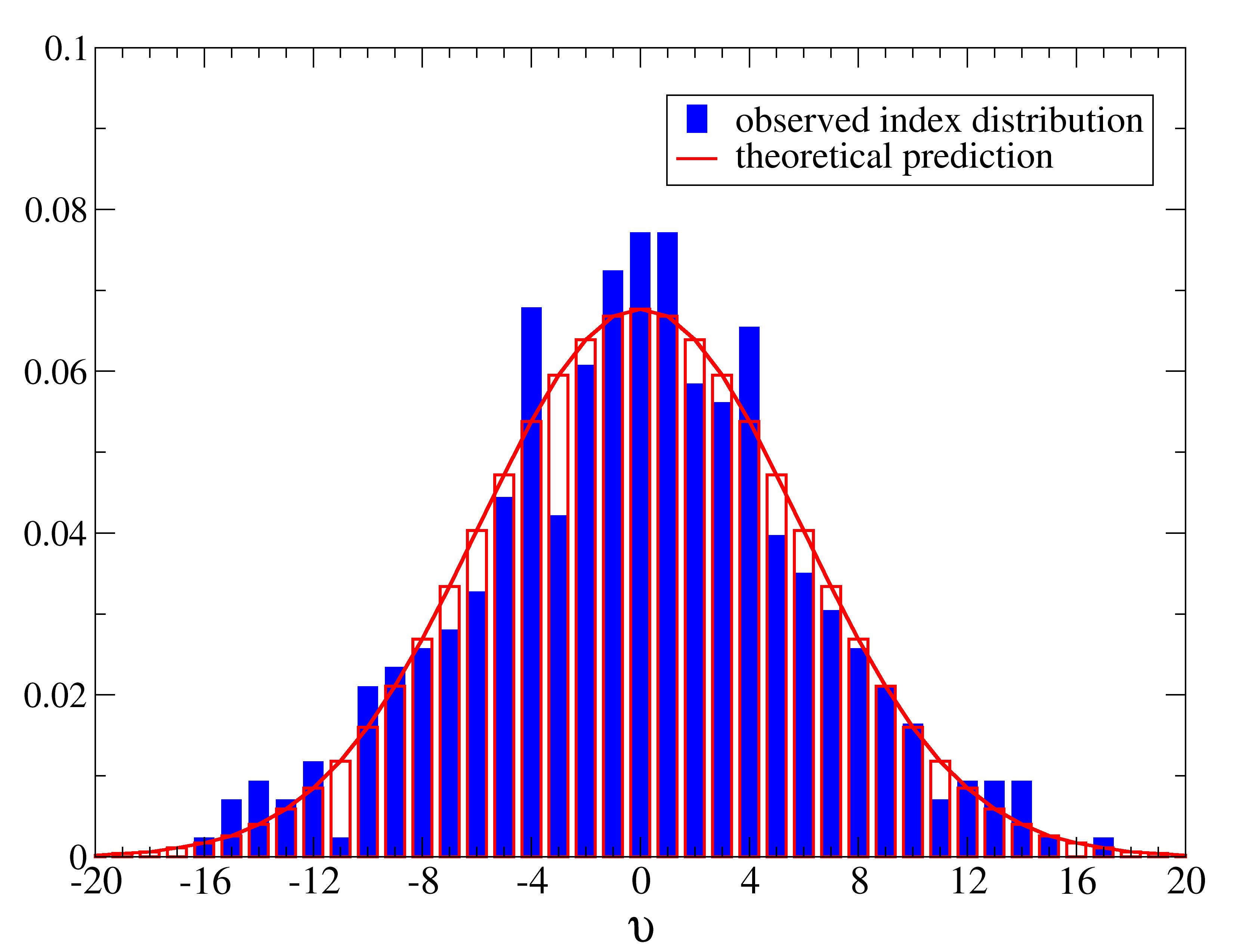
Figure 1: (Normalised) distribution of the index $\nu$ of the Neuberger-Dirac operator in the gauge ensemble used for our $\epsilon$-regime computations (blue histogram), compared to the gaussian shape expected in infinite volume (in red). The width of the gaussian has been computed with the value of the topological susceptibility $r_{0}^{4}\chi=0.00715(22)$ from [56]. Note that the comparison does thus not involve any free parameter.

Our simulations are carried out in the quenched approximation, on a single lattice of size $32\times 16^{3}$ at $\beta=5.8485$. This corresponds to a lattice spacing given, in terms of the Sommer parameter $r_{0}\approx 0.5~{}{\rm fm}$, by $a/r_{0}\simeq 0.247$ [57]. We always consider degenerate values of the light quark masses, $m_{u}=m_{d}=m_{s}\equiv m_{l}$. Our simulation points are given in the first two columns of Table 1. For the light masses we consider one $\epsilon$-regime point ($am_{l}=0.002$) and two $p$-regime points ($am_{l}=0.020,0,030$); the pseudoscalar octet meson masses for the latter, measured from the two-point function of the non-singlet left-handed current, are quoted in the third column of Table 1. For each light point then we consider a value $m_{c}=m_{l}$, corresponding to the GIM limit, and two heavier charm masses $am_{c}=0.040$ and $am_{c}=0.200$; for $am_{l}=0.020$ we also consider an even heavier mass $am_{c}=0.400$. The value $am_{c}=0.040$ is still expected to be within the reach of ChiPT, thus lying in the validity range of the study in [33]. Taking $r_{0}=0.5~{}{\rm fm}$ and the value of $a/r_{0}$ quoted before, our $p$-regime light pseudoscalar meson masses correspond to $m_{\rm PS}\approx 317~{}{\rm MeV}$ and $m_{\rm PS}\approx 371~{}{\rm MeV}$. Using also the value $\widehat{Z}_{\rm S}\simeq 1.28$ for the RGI scalar renormalisation constant from [58], our three RGI charm masses for simulations at $m_{c}\neq m_{l}$ correspond, respectively, to $M_{c}\approx 50$, $249$, and $498~{}{\rm MeV}$. Note that, while the scaling properties of computations with overlap fermions are generally expected to be good, at the heaviest charm mass $am_{c}=0.400$ cutoff effects can be expected to be sizeable.

For each of the three values of $m_{l}$ we have an independent ensemble of around 400 independent gauge configurations. Only about half the statistics is used for the computation at $am_{c}=0.4$, as well as in the computation of three-point functions involving $Q_{2}^{\pm}$.

4.2 Variance reduction techniques

Our main aim is to compute the two- and three-point functions involved in the matching of QCD to ChiPT, as discussed in Section 2. After integrating over fermion variables in the path integral, fermionic correlation functions can be written as usual in terms of gauge expectation values of traces of products of quark propagators and spin matrices; explicit expressions are provided in Appendix B. The reason to consider left-handed currents as interpolating operators becomes apparent in that the traces only contain left-handed propagators $P_{-}S(x,y)P_{+}$, that can always be computed in the chirality sector that does not contain zero modes, thus avoiding their contribution in correlators [54]. The three-point functions involving $Q_{1}^{\pm}$ require the computation of the quark-propagator diagrams depicted in Fig. 2, to which we will refer as “eight” and “eye” diagrams, respectively. Each of them appears in a colour-spin connected and a colour-spin disconnected version.

The computation of these correlation functions poses severe problems in terms of noise-to-signal ratio. When the light quark mass is sufficiently low (and especially so in the $\epsilon$-regime), Dirac modes with very small eigenvalues have large contributions to correlation functions. Their wavefunctions have been shown to develop localised structures [59], which makes good sampling of the whole lattice volume mandatory in order to avoid large statistical fluctuations. It is thus important to integrate over space at all operator insertion points (or at least at as many insertions as possible), which obviously cannot be achieved with propagators computed with point sources. The use of all-to-all propagators for variance reduction thus becomes mandatory.

Figure 2: Eight and eye diagrams appearing in the computation of three-point functions of $Q_{1}^{\pm}$.

One first step in this direction was the development of low-mode averaging (LMA) in [60, 61]. In this particular brand of LMA the Dirac propagator $S$ is split into the contribution $S_{l}$ from the lowest-lying $N_{\rm low}$ modes, which are treated exactly, and its orthogonal complement $S_{h}$, which is computed with a point source. This in turn implies a split of correlation functions into $2^{\rm L}$ different contributions, where ${\rm L}$ is the number of propagators involved. Contributions to correlation functions where two low propagators meet at an operator insertion point can be integrated over space, since $S_{l}$ is effectively an all-to-all propagator. On top of that, extra inversions performed using low modes as sources allow to integrate also at insertions where one $S_{l}$ and one $S_{h}$ meet. This was exploited in [61] to determine chiral LECs in the $\epsilon$-regime, and in [62, 30] to determine the weak LECs $g_{1}^{\pm}$ in the GIM $m_{c}=m_{u}$ limit, implying that the noise-to-signal problem for eight diagrams is tamed via LMA.

The same techniques are however insufficient when applied to eye contractions; in particular, the LMA technique does not allow to integrate over space at the insertion of the four-fermion operator when $S_{h}$ circulates in the closed loop. One thus needs to combine LMA with other variance reduction techniques, such as stochastic volume sources (SVS) [63, 64], and the novel probing algorithm proposed in [65]; the latter can be used specifically for the precise computation of closed propagators. A thorough study of these techniques applied to our problem has been conducted in a companion paper [32], where the very large impact on variance reduction, at an affordable computational cost, has been demonstrated. In the present work, we have employed the optimised combination of LMA with SVS developed in [32], to which we refer for full details, with the specific aim of obtaining a well-behaved signal for the eye diagram. The specific setup employed here treats the $20$ lowest modes of the Dirac operator exactly, and estimates $S^{h}$ with SVS using time and spin-colour dilution and two stochastic hits.

In the case of the three-point function involving $Q_{2}^{\pm}$, a contribution from the spin-diagonal part of the operator is unavoidable, since the presence of (pseudo)scalar densities implies that not all propagators are left-handed. LMA has not been implemented for these diagrams, and the only variance reduction techniques we employ for them is the used of extended propagators, which allows to integrate over space at two of the three operator insertions. On the other hand, for this correlation function the prediction in Eq. (3.48) is expected to be accurate up to small NLO ChiPT corrections for light quark masses in the $p$-regime; we can thus use the latter, together with the numerical results, to provide a solid estimation.

4.3 Results for ratios of correlation functions

Sufficiently far away from operator insertions, the ratios involved in the matching to ChiPT can be fitted to a plateau ansatz so that correlation functions are dominated by the contribution from the lightest state. Details about the fits are provided in Appendix D; our final results are quoted in Table 1. Ratios in the $\epsilon$-regime are first computed in a fixed topological sector $|\nu|$, and then a weighted average of the results for various values of $|\nu|$ is taken. This procedure is based on the ChiPT prediction that the ratios are insensitive to the value of $|\nu|$ up to NNLO corrections. The results in Table 1 include the topological sectors $3\leq|\nu|\leq 7$. This choice takes into account that no signal for eye diagrams is found for $|\nu|<3$, and considering $|\nu|>7$ can be expected to introduce large finite volume effects. Fig. 3 illustrates the $|\nu|$ dependence of our results. The number of gauge configurations in the averages for each value of $|\nu|$ is $\{42,57,36,29,25\}$, respectively.

$(am_{l}\,,\,am_{c})$	$am_{\rm PS}$	$R_{1}^{+}$	$R_{1}^{-}$	$R_{u}^{+}$	$R_{2}^{\pm}$	$R_{2}^{\pm;{\rm ChiPT}}$
0.002 , 0.002	—	0.629(77)	2.09(25)	0.503(62)	0	0
0.002 , 0.040	—	0.686(78)	2.46(16)	0.503(62)	n/a	-0.51(19)
0.002 , 0.200	—	0.73(12)	2.68(13)	0.503(62)	n/a	-13(4)
0.020 , 0.020	0.1986(20)	0.692(25)	1.972(63)	0.554(20)	0	0
0.020 , 0.040	0.1986(20)	0.717(25)	2.028(64)	0.554(20)	-0.36(12)	-0.38(7)
0.020 , 0.200	0.1986(20)	0.766(32)	2.220(82)	0.554(20)	-12(4)	-13(3)
0.020 , 0.400	0.1986(20)	0.767(51)	2.42(12)	0.554(20)	-48(16)	-51(9)
0.030 , 0.030	0.2322(19)	0.731(22)	1.829(64)	0.585(18)	0	0
0.030 , 0.040	0.2322(19)	0.746(22)	1.852(64)	0.585(18)	n/a	-0.22(4)
0.030 , 0.200	0.2322(19)	0.835(31)	1.953(82)	0.585(18)	n/a	-13(3)

Table 1: Bare quark masses, light pseudoscalar meson masses, and results for the ratios of QCD correlation functions involved in the matching to ChiPT.

In the case of the ratio $R_{2}^{\pm}$, numerical results are provided in Table 1 for $am_{l}=0.020$ only. We also provide the LO ChiPT prediction for all kinematical points in the $p$-regime, using Eq. (3.49) with the bare values of quark masses. The central value is set using $Fr_{0}=0.275(6)$ from [66], and a systematic uncertainty that mimics the impact of NLO corrections, obtained by varying $Fr_{0}$ in the range $0.250\lesssim Fr_{0}\lesssim 0.300$, is assigned. This is a fairly conservative error estimate, as shown by the discussion in Appendix A. The current normalisation factor $Z_{\rm\scriptscriptstyle A}^{2}$ needed to make connection with the ChiPT prediction (cf. Section 3) is $Z_{\rm\scriptscriptstyle A}=1.706(5)$, taken from [66]. Finally, by assuming that Eq. (3.49) remains valid in the $\epsilon$-regime, we also provide estimates of $R_{2}^{\pm}$ for the point $am_{l}=0.002$. This assumption can be argued to hold on the basis of the smooth $m_{l}\to 0$ limit of the relevant ChiPT formula for ${\cal R}_{8}$, that provides the $\epsilon$-regime value. In order to allow for possible larger NLO (finite volume) corrections in this case, we have doubled the size of the error estimate.

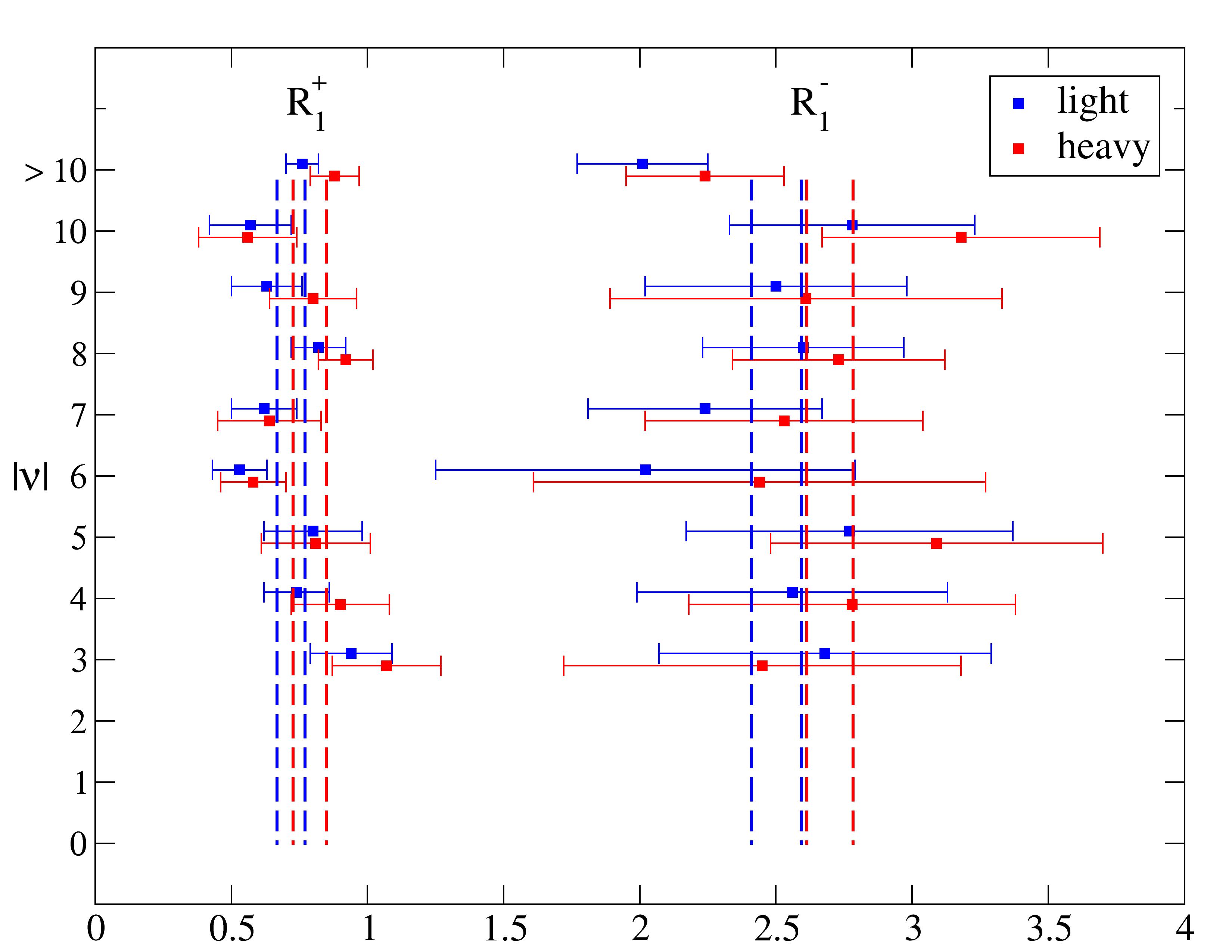
Figure 3: Values of the ratios $R_{1}^{\pm}$ in the $\epsilon$-regime as a function of $|\nu|$. “Light” and “heavy” refer to results for $am_{c}=0.040$ and $am_{c}=0.200$, respectively.

For the simulation points where a direct comparison is possible, the ChiPT prediction is remarkably consistent with lattice data, within the relatively large errors displayed by both quantities. Decreasing these errors would require a dedicated variance reduction study, similar to the one conducted for correlators involving four-fermion operators. Since, on the other hand, the contribution of $R_{2}^{\pm}$ to physical amplitudes is suppressed by the small subtraction coefficients $c^{\pm}$, as discussed above, the level of precision displayed by our results for $R_{2}^{\pm}$ in Table 1 is good enough for the purpose of the present work. We will henceforth take as input the values in the last column of Table 1 in the construction of the subtracted amplitudes.

In Table 2 we provide results for the ratios of the correlation functions $D_{1}^{\pm}/D_{2}^{\pm}$ introduced in Eq. (3.51), which are expected to exhibit plateaux that can be fitted for the subtraction coefficients $c^{\pm}$. As explained in section 3, the dominant contribution in the $p$-regime comes from scalar-to-vacuum amplitudes, which makes this quantity very noisy — indeed no signal is found from our data. The same applies to the ratios computed in the $\epsilon$-regime, where the correlation functions do receive contributions from the pseudoscalar channel but the intrinsic statistical fluctuations are also larger. We are thus unable to provide a solid non-perturbative estimate of subtraction coefficients. On the other hand, the error intervals we find are compatible with the expectation $c^{\pm}\sim{\cal O}(\alpha_{\rm s}/(4\pi))$.

In order to treat the contribution from the subtraction safely, we thus proceed as follows. Subtraction coefficients are treated as suggested by the one-loop analysis of Section 3 — i.e. set to zero, with a systematic uncertainty given by $\alpha^{{\overline{\rm MS}}}_{\rm s}(1/a)/(4\pi)\sim 0.028$. When used together with the estimate of the subtraction term coming from ChiPT, this leads to a systematic uncertainty on renormalised $K\to\pi$ amplitudes, that should safely cover the effect of subtractions. As the charm mass increases, the total error becomes increasingly dominated by this uncertainty. However, the relative error on the final result is still around or below $20\%$ for $am_{c}\leq 0.2$, and becomes very large only for $am_{c}=0.4$. Using the values of the renormalisation factors from [40] quoted in Table 3, this leads to the renormalised ratios in Table 4, that can then be used for the matching to ChiPT.

$(am_{l}\,,\,am_{c})$	$am_{\rm PS}$		$c^{+}$		$c^{-}$
0.002 , 0.040	—		0.05(4)	-	0.14(48)
0.002 , 0.200	—		0.00(3)	-	0.01(3)
0.020 , 0.040	0.1986(20)	-	0.01(12)	-	0.08(10)
0.020 , 0.200	0.1986(20)		0.00(1)		0.00(9)
0.030 , 0.040	0.2322(19)		0.04(10)		0.14(48)
0.030 , 0.200	0.2322(19)		0.01(21)		0.02(8)

Table 2: Numerical results for the subtraction coefficients $c^{\pm}$, obtained from the ratios of correlation functions in Eq. (3.51).

$\sigma$	$k_{1}^{\sigma;{\rm RGI}}$	$U_{1}^{\sigma}(\mu/\Lambda)\frac{Z_{11}^{\sigma}(\mu)}{Z_{\rm\scriptscriptstyle A}^{2}}$	${\cal Z}_{1}^{\sigma}$
$+$	0.7080	1.15(12)	0.81(8)
$-$	1.9775	0.561(61)	1.11(12)

Table 3: Values of Wilson coefficients and renormalisation factors for quenched QCD at $\beta=5.8485$ (from [40]).

5 Matching to Chiral Perturbation Theory

In order to determine the values of $g_{8}(m_{c})$ and $g_{27}(m_{c})$, the renormalised QCD quantities $R_{27},R_{8}$ in Table 4 and the ChiPT ratios ${\cal R}_{27},{\cal R}_{8}$ in Appendix A have to be introduced into Eqs. (2.38,2.39), for each of the values of $m_{c}$ available, apart from $am_{c}=0.4$ — for which we have results only at one value of the light mass, and errors are large. As already noted, our results in the GIM limit are well-consistent with those in [30] for the same simulations points — differences are always below the $2\sigma$ level.

$(am_{l}\,,\,am_{c})$	$am_{\rm PS}$	$R_{27}$	$R_{8}$
0.002 , 0.002	—	0.407(69)	2.42(38)
0.002 , 0.040	—	0.407(69)	2.88(35)
0.002 , 0.200	—	0.407(69)	3.16(62)
0.020 , 0.020	0.1986(20)	0.449(48)	2.30(25)
0.020 , 0.040	0.1986(20)	0.449(48)	2.38(26)
0.020 , 0.200	0.1986(20)	0.449(48)	2.64(58)
0.020 , 0.400	0.1986(20)	0.449(48)	2.9(2.0)
0.030 , 0.030	0.2322(19)	0.474(50)	2.15(23)
0.030 , 0.040	0.2322(19)	0.474(50)	2.19(23)
0.030 , 0.200	0.2322(19)	0.474(50)	2.36(56)

Table 4: Renormalised QCD ratios that enter the matching to ChiPT.

A straightforward procedure follows by rewriting Eqs. (2.38,2.39) as

$$\begin{split}R_{27}(m_{l},m_{c})&=g_{27}(m_{c})\left\{1-\Delta_{27}[m_{l},\Lambda_{27}(m_{c})]\right\}\,,\\ R_{8}(m_{l},m_{c})&=g_{8}(m_{c})\left\{1-\Delta_{8}[m_{l},\Lambda_{8}(m_{c})]\right\}\,,\end{split}$$ (5.67)

where for greater clarity we have made quark mass dependences explicit. Here $\Delta_{k}(m_{l})$ is either the NLO (finite-volume) correction in the $\epsilon$-regime (for which effectively $m_{l}=0$),

$$\Delta_{27}^{\epsilon}=0.182(8)\,,~{}~{}~{}~{}~{}~{}~{}~{}~{}~{}~{}~{}~{}\Delta_{8}^{\epsilon}=-0.273(12)\,.$$ (5.68)

or the $p$-regime correction involving chiral logs plus finite-volume terms. The scales $\Lambda_{k}$ parametrise contributions from NLO terms in the $p$-regime chiral effective Hamiltonian. By setting $Fr_{0}=0.275(6)$, one can then fit our three $m_{l}$ data points, separately in the 27-plet and octet channels and for each value of $m_{c}$, to determine the two parameters $g_{k}(m_{c})$ and $\Lambda_{k}(m_{c})$. Note that all the data points come from different gauge ensembles, which makes their correlation negligible.

As discussed in Section 2, the matching to ${\rm SU}(3)$ ChiPT of quenched results is problematic in the octet case. In particular, singlet contributions to the formulae in Appendix A should be taken into account. Since, on the other hand, the errors on $R_{8}$ are large, and we only have results at two $p$-regime quark masses, the sensitivity to these NLO effects is very poor. We have fit our numbers to the $N_{\rm f}=2$, $N_{\rm f}=3$, and $N_{\rm f}=4$ formulae, and find that the value of $g_{8}$ is completely insensitive to $N_{\rm f}$; only $\Lambda_{8}$ changes, as shown in Table 5. The result we thus quote for the LO LECs is

$$\begin{array}[]{l@{\hspace{10mm}}r@{\hspace{1mm}}c@{\hspace{1mm}}l@{\hspace{5mm}}r@{\hspace{1mm}}c@{\hspace{1mm}}l}am_{c}=0.00:\hfil\hskip 28.45274pt&g_{27}\hskip 2.84526pt&=\hfil\hskip 2.84526pt&0.50(8)\,,\hfil\hskip 14.22636pt&g_{8}\hskip 2.84526pt&=\hfil\hskip 2.84526pt&1.9(3)\,;\\[8.61108pt] am_{c}=0.04:\hfil\hskip 28.45274pt&g_{27}\hskip 2.84526pt&=\hfil\hskip 2.84526pt&0.50(8)\,,\hfil\hskip 14.22636pt&g_{8}\hskip 2.84526pt&=\hfil\hskip 2.84526pt&2.3(3)\,;\\[8.61108pt] am_{c}=0.20:\hfil\hskip 28.45274pt&g_{27}\hskip 2.84526pt&=\hfil\hskip 2.84526pt&0.50(8)\,,\hfil\hskip 14.22636pt&g_{8}\hskip 2.84526pt&=\hfil\hskip 2.84526pt&2.5(5)\,,\\ \end{array}$$ (5.72)

where we have also included (labeling it as $m_{c}=0$) the result of a reanalysis of the GIM limit based on our simulations. The latter is again consistent within $\sim 1\sigma$ with the conclusions in [30]. Recall that, since we are working in the quenched approximation, the LEC $g_{27}$ is strictly independent of $m_{c}$. These fit results are illustrated in Fig. 4.

$N_{\mathrm{\scriptstyle f}}$	$am_{c}$	$g_{8}$	$\Lambda_{8}$
2	0.00	1.92(28)	0.28(9)
3	0.00	1.94(28)	0.32(16)
4	0.00	1.94(29)	0.37(26)
2	0.04	2.26(26)	0.22(5)
3	0.04	2.28(26)	0.22(8)
4	0.04	2.59(11)	0.26(11)
2	0.20	2.49(47)	0.22(9)
3	0.20	2.50(48)	0.21(14)
4	0.20	2.50(48)	0.21(20)

Table 5: Results of fits to ChiPT formulae for $g_{8}$ and $\Lambda_{8}$. (See text for an explanation of the $N_{\mathrm{\scriptstyle f}}$ dependence of the fit function; the $\epsilon$-regime point is labeled $am_{c}=0.00$; the (correlated) $\chi^{2}/{\rm d.o.f.}$ of the fits is always $\lesssim 10^{-2}$.)

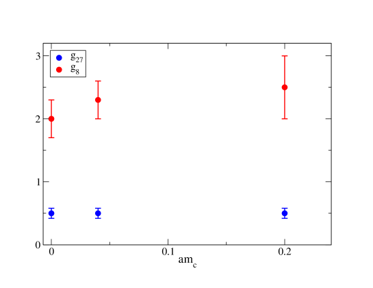
Figure 4: LO LECs $g_{27}$ and $g_{8}$ as a function of $am_{c}$. Recall the “experimental” values $g_{27}\sim 0.50$ and $g_{8}\sim 10.5$ (cf. Section 2).

Alternatively, as discussed in [30], fits can be performed to the product $R_{27}R_{8}$, which is less sensitive to chiral corrections, and take the value of $g_{27}(0)$ as input from the more solid determination in that work (which has better $\epsilon$-regime statistics and additional $p$-regime masses). The fit ansatz for the product of ratios is

$$R_{27}\,R_{8}=g_{27}g_{8}[1-\tilde{\Delta}]\,,$$ (5.73)

where $\tilde{\Delta}=\Delta_{27}+\Delta_{8}$ — explicitly

$$\begin{split}\tilde{\Delta}^{\epsilon}&=-0.091(4)\,,\\ \tilde{\Delta}^{p}&=-\frac{M^{2}}{(4\pi F)^{2}}\left[\left(8+\frac{10}{N_{\rm f}}\right)\log\left(\frac{M^{2}}{\tilde{\Lambda}^{2}}\right)-({\cal V}_{27}+{\cal V}_{8})\right]\,,\end{split}$$ (5.74)

where $\tilde{\Lambda}$ is a single scale that combines the effect of NLO terms in the 27-plet and octet channel (cf. Appendix A for unexplained notation). We follow the same procedure to check the dependence on $N_{\rm f}$ as before, finding similar results. The outcome of this latter fit strategy is

$$\begin{array}[]{l@{\hspace{10mm}}r@{\hspace{1mm}}c@{\hspace{1mm}}l}am_{c}=0.00:\hfil\hskip 28.45274pt&g_{27}g_{8}\hskip 2.84526pt&=\hfil\hskip 2.84526pt&0.94(2)\,;\\[4.30554pt] am_{c}=0.04:\hfil\hskip 28.45274pt&g_{27}g_{8}\hskip 2.84526pt&=\hfil\hskip 2.84526pt&1.10(2)\,;\\[4.30554pt] am_{c}=0.20:\hfil\hskip 28.45274pt&g_{27}g_{8}\hskip 2.84526pt&=\hfil\hskip 2.84526pt&1.20(4)\,,\end{array}$$ (5.78)

which exhibits good consistency with the results in Eq. (5.72), and checks that they are robust.

6 Conclusions

In this paper we have explored the behaviour of the $K\to\pi\pi$ decay amplitudes involved in the $\Delta I=1/2$ rule as a function of the charm quark mass, following the strategy laid out in [28]. The aim is to understand the role of the charm quark in the $\Delta I=1/2$ enhancement. Our work extends the results for the GIM limit $m_{c}=m_{u}$ in [30, 31]. The numerical techniques developed in [32] have been instrumental in the lattice QCD computation of amplitudes involving eye diagrams.

Our main finding is that unsubtracted matrix elements of the four-fermion operators $Q_{1}^{\pm}$, computed in quenched QCD, have a mild dependence on the charm-up quark mass difference across the regime where the charm quark becomes heavy. Indeed, while our simulations do not reach the physical value of the charm mass, they cover values of $m_{c}$ about 100 times larger than the physical value of $(m_{u}+m_{d})/2$. At that point, the dominant contribution to the enhancement from $Q_{1}^{-}$ increases by no more than $\sim 30\%$ with respect to the value found with light and mass-degenerate up and charm quarks.

We have also discussed how the subtraction term needed to obtain the physical amplitudes for $m_{c}\neq m_{u}$ is proportional to $m_{c}^{2}$ for a heavy charm. Combined with the above result, this would imply that the ratio of low-energy couplings $g_{8}/g_{27}$ is bound to become large as the charm mass increases, since the contribution from the subtraction term will eventually dominate. Alternatively, bare matrix elements of $Q_{1}^{\pm}$ may start showing a larger $m_{c}$ dependence closer to the physical charm mass value, allowing for potential cancellations. This however seems unnatural, since, as pointed above, our $m_{c}$ values are already well above the light quark regime. In that sense, our results point in the direction of supporting that a strong enhancement is natural for large enough values of $m_{c}/m_{u}$.

On the other hand, our results are insufficient to determine the contribution from the subtraction term precisely. While the value of the matrix elements of the operator $Q_{2}^{\pm}$ involved in the subtraction are well-controlled (within sizeable uncertainties), further work is needed for a reliable non-perturbative determination of the subtraction coefficients $c^{\pm}$. In the interpretation that the $m_{c}$ dependence at large $m_{c}$ is driven by the subtraction term, the value of $c^{\pm}$ is crucial to fix the precise value of $|A_{0}|/|A_{2}|$ at the physical point. Assuming the suppression in $c^{\pm}$ hinted at by perturbation theory, we have found that the enhancement already observed in the GIM limit does not increase significantly within the range of values of $m_{c}$ covered by our simulations. The ultimate question whether Standard Model physics alone can quantitatively explain the experimental value of $|A_{0}|/|A_{2}|$ is thus left open — answering it within our framework still requires a more detailed study of the subtraction terms, as well as reaching out to values of the charm mass in the physical region.

A Chiral Perturbation Theory formulae

In this appendix we collect the essential next-to-leading order quenched ChiPT formulae from [28, 33] relevant for the determination of the LECs in the ${\rm SU}(4)$ and ${\rm SU}(3)$ chiral effective weak Hamiltonians. We also discuss NLO ChiPT corrections to the ratio $(m_{K}^{2}-m_{\pi}^{2})/(m_{s}-m_{d})$ that determines matrix elements of $Q_{2}^{\pm}$ in our kinematics.

A.1 NLO corrections to chiral weak Hamiltonians

Here we provide NLO results for the various ratios of correlation functions in ChiPT discussed in the text, taken from [33]. Note that $\epsilon$-regime results are given for a specific topological sector with topological charge $\nu$. In particular, the ratios ${\cal R}_{1}^{\pm},{\cal R}_{27},{\cal R}_{8}$ happen to be independent of $\nu$ up to NNLO corrections, while the expressions involving the unphysical operator ${\cal O}^{\prime}_{8}$ do exhibit topology dependence, but they are not included here since their explicit form is not needed in the matching. In $p$-regime expressions, the contributions from unknown NLO LECs are included in the scales appearing in chiral logarithms. For ${\rm SU}(3)$ ChiPT in the octet channel we quote the unquenched formulae; comments about the matching to quenched QCD results are provided in Section 2 and Section 5.

All equations hold in a box with four-volume $V=L^{3}\times T$ and aspect ratio $\rho=T/L$. The dependence on the light quark mass $m_{l}$ is given either in terms of the leading-order Goldstone boson mass $M^{2}=2\Sigma m_{l}/F^{2}$ ($p$-regime), or in terms of the dimensionless parameter $\mu=m_{l}\Sigma V$ ($\epsilon$-regime).

${\rm SU}(4)$ ChiPT, $\epsilon$-regime:

$${\cal R}_{1;\nu}^{\pm}(x_{0},y_{0})=1\pm\,\frac{2}{F^{2}T^{2}}\,(\beta_{1}\rho^{3/2}-k_{00}\rho^{3})\,.$$ (A.79)

${\rm SU}(3)$ ChiPT, $\epsilon$-regime:

$${\cal R}_{27;\nu}(x_{0},y_{0}) =1+\,\frac{2}{F^{2}T^{2}}\,(\beta_{1}\rho^{3/2}-k_{00}\rho^{3})\,,$$ (A.80)

$${\cal R}_{8;\nu}(x_{0},y_{0}) =1-\,\frac{3}{F^{2}T^{2}}\,(\beta_{1}\rho^{3/2}-k_{00}\rho^{3})\,.$$ (A.81)

${\rm SU}(4)$ ChiPT, $p$-regime:

$${\cal R}_{1}^{\pm}(x_{0},y_{0})=1\pm\frac{M^{2}}{(4\pi F)^{2}}\left[3\log\left(\frac{M^{2}}{\Lambda_{\pm}^{2}}\right)\mp{\cal V}_{1}(x_{0},y_{0})\right]\,.$$ (A.82)

${\rm SU}(3)$ ChiPT, $p$-regime:

$${\cal R}_{27}(x_{0},y_{0}) =1+\frac{M^{2}}{(4\pi F)^{2}}\left[3\log\left(\frac{M^{2}}{\Lambda_{27}^{2}}\right)-{\cal V}_{27}(x_{0},y_{0})\right]\,,$$ (A.83)

$${\cal R}_{8}(x_{0},y_{0}) =1+\frac{M^{2}}{(4\pi F)^{2}}\left[\left(\frac{1}{2}-\frac{10}{N_{\rm f}}\right)\log\left(\frac{M^{2}}{\Lambda_{8}^{2}}\right)-{\cal V}_{8}(x_{0},y_{0})\right]\,.$$ (A.84)

Finite volume effects:

NLO corrections in the $\epsilon$-regime are pure finite-volume effects, parametrised by the geometrical coefficients [67, 68, 48]

$$\beta_{1} =\frac{1}{4\pi}\left[2-\hat{\alpha}_{-1}(\rho^{3/4},\rho^{-1/4})-\hat{\alpha}_{-1}(\rho^{-3/4},\rho^{1/4})\right]\,,$$ (A.85)

$$k_{00} =\frac{1}{12}-\frac{1}{4}\sum_{\mathbf{n}\neq\mathbf{0}}\frac{1}{\sinh^{2}(\pi\rho|\mathbf{n}|)}\,,$$ (A.86)

where $\mathbf{n}$ are integer vectors, and $\hat{\alpha}_{p}$ is given in terms of the elliptic theta function $S(x)=\sum_{n=-\infty}^{\infty}\exp(-\pi xn^{2})=\vartheta_{3}(0,\exp(-\pi x))$ by

$$\hat{\alpha}_{p}(l_{0},l_{i})=\int_{0}^{1}{\rm d}t\,t^{p-1}\left[S(l_{0}^{2}/t)S^{3}(l_{i}^{2}/t)-1\right]\,.$$ (A.87)

A table with sample values of $\beta_{1},k_{00}$ is provided in Table 4 of [28]. In our lattice,

$$\beta_{1}=0.08360\,,~{}~{}~{}~{}~{}~{}~{}~{}~{}~{}~{}~{}~{}~{}~{}~{}~{}~{}~{}~{}~{}k_{00}=0.08331.$$ (A.88)

This implies, in particular, that the parameter that controls $\epsilon$-regime NLO corrections is $(\beta_{1}\rho^{3/2}-k_{00}\rho^{3})/(F^{2}T^{2})\approx-0.13$, taking $F\approx 90~{}{\rm MeV}$ and $T\approx 4~{}{\rm fm}$. That implies large corrections ranging between $\sim 25\%$ and $\sim 40\%$ in the $\epsilon$-regime matching for LECs.

Finite-volume effects in $p$-regime ratios involving three-point functions are given, in sufficiently large volumes, by

$${\cal V}_{1}(x_{0},y_{0})={\cal V}_{27}(x_{0},y_{0}) =e^{-2M|x_{0}|}\phi_{1}(2M|x_{0}|)+e^{-2M|y_{0}|}\phi_{1}(2M|y_{0}|)\,,$$ (A.89)

$${\cal V}_{8}(x_{0},y_{0}) =e^{-2M|x_{0}|}\phi_{2}(2M|x_{0}|)+e^{-2M|y_{0}|}\phi_{2}(2M|y_{0}|)\,,$$ (A.90)

with

$$\phi_{1}(x) =\int_{0}^{\infty}{\rm d}z\,e^{-xz}\frac{\sqrt{z(2+z)}}{1+z}\left[\frac{1}{2+z}+\frac{1}{1+z}-2\right]\,,$$ (A.91)

$$\phi_{2}(x) =\int_{0}^{\infty}{\rm d}z\,e^{-xz}\frac{\sqrt{z(2+z)}}{1+z}\left[\frac{-4+\frac{5}{N_{\rm f}}}{2+z}+\frac{1-\frac{5}{N_{\rm f}}}{1+z}-2+\frac{10}{N_{\rm f}}-\left(10-\frac{20}{N_{\rm f}}\right)z\right]\,.$$ (A.92)

Note that the dependence of these quantities on $(x_{0},y_{0})$ is actually very mild; in fits we will take their values at $x_{0}=-y_{0}=T/3$.

A.2 NLO corrections to $(m_{K}^{2}-m_{\pi}^{2})/(m_{s}-m_{d})$

The full NLO expression for the ratio $(m_{K}^{2}-m_{\pi}^{2})/(m_{s}-m_{d})$ is given by [69] (we take $m_{u}=m_{d}$ throughout; general expressions can be obtained by replacing occurrences of $m_{d}$ by $m_{ud}={\scriptstyle{{1\over 2}}}(m_{u}+m_{d})$)

$$\begin{split}\frac{m_{K}^{2}-m_{\pi}^{2}}{m_{s}-m_{d}}=\frac{\Sigma_{0}}{F_{0}^{2}}\bigg{\{}1&+\frac{\Sigma_{0}}{8\pi^{2}F_{0}^{4}}\left[(m_{s}+m_{d})\,\ell_{1}+m_{d}\,\ell_{2}\right]\\ &+\frac{8\Sigma_{0}}{F_{0}^{4}}\left[(m_{s}+3m_{d})(2L_{8}-L_{5})+2(m_{s}+2m_{d})(2L_{6}-L_{4})\right]\bigg{\}}\,,\end{split}$$ (A.93)

where $F_{0},\Sigma_{0},L_{i}$ are the standard ${\rm SU}(3)$ LECs, and the logarithm terms $\ell_{1,2}$ read

$$\ell_{1} =\frac{2}{9}\log\left[\frac{2\Sigma_{0}(2m_{s}+m_{d})}{3\mu^{2}F_{0}^{2}}\right]\,,$$ (A.94)

$$\ell_{2} =\left(\frac{m_{s}}{m_{s}-m_{d}}\right)\log\left[\frac{2\Sigma_{0}(2m_{s}+m_{d})}{3\mu^{2}F_{0}^{2}}\right]-\left(\frac{m_{d}}{m_{s}-m_{d}}\right)\log\left[\frac{2\Sigma_{0}m_{d}}{\mu^{2}F_{0}^{2}}\right]\,.$$ (A.95)

Following standard practice, we assume $\mu=770~{}{\rm MeV}$ as the scale at which the logarithms, quark masses, and NLO LECs $L_{i}$ are evaluated. The term $\ell_{2}$ does not transparently have a well-behaved $m_{s}=m_{d}$ limit, but it is easy to show that taking $m_{s}=m_{d}(1+\epsilon)$ one can write it as

$$\ell_{2}=\frac{2}{3}+\log\left[\frac{2\Sigma_{0}m_{d}}{\mu^{2}F_{0}^{2}}\right]\,+\,{\cal O}(\epsilon)\,.$$ (A.96)

The result for $m_{s}=m_{d}=m_{u}\equiv m_{l}$ simplifies to

$$\begin{split}\frac{m_{K}^{2}-m_{\pi}^{2}}{m_{s}-m_{d}}\to\frac{\Sigma_{0}}{F_{0}^{2}}\bigg{\{}1&+\frac{\Sigma_{0}m_{l}}{8\pi^{2}F_{0}^{4}}\left(\frac{2}{3}+\frac{13}{9}\log\left[\frac{2\Sigma_{0}m_{l}}{\mu^{2}F_{0}^{2}}\right]\right)\\ &+\frac{16\Sigma_{0}m_{l}}{F_{0}^{4}}\left[2(2L_{8}-L_{5})+3(2L_{6}-L_{4})\right]\bigg{\}}\,.\end{split}$$ (A.97)

In the quenched case there will be additional contributions from the non-decoupled singlet terms, which can be reabsorbed in a renormalised chiral condensate $\bar{\Sigma}_{0}$, that will diverge in the chiral limit.

Current reference values for the relevant LECs, obtained from $N_{f}=2+1$ lattice simulations, are [70, 71, 72, 73]

$$\begin{split}F_{0}=80(6)~{}{\rm MeV}\,,&~{}~{}~{}~{}~{}~{}~{}~{}~{}\Sigma_{0}^{1/3}=245(8)~{}{\rm MeV}\,,\\ (2L_{6}-L_{4})=0.03^{+40}_{-36}\times 10^{-3}\,,&~{}~{}~{}~{}~{}~{}~{}~{}~{}(2L_{8}-L_{5})=-0.15^{+46}_{-22}\times 10^{-3}\,.\end{split}$$ (A.98)

This implies $\Sigma_{0}/F_{0}^{4}\simeq 0.36(11)~{}{\rm MeV}^{-1}$, and therefore a conservative upper bound for the size of NLO corrections for values of $m_{l}\lesssim m_{s}^{\rm phys}/4$, as is our case, can be taken to be $\sim 5\%$, which we increase to $\sim 10\%$ to account for deviations from this scenario in the quenched case (which can be expected to be small, as shown by the values for LO quenched LECs derived from a similar lattice setup to the one used in this work [66]).

B Wick contractions for QCD correlation functions

B.1 Three-point functions of $Q_{1}^{\pm}$

In the limit $m_{u}=m_{d}=m_{s}=m_{l}$, the QCD three-point functions involving $Q_{1}^{\pm}$ needed in our setup can be computed in terms of a few independent fermionic traces. Without loss of generality, we will write the expressions for a four-fermion operator inserted at $z=0$. Let $S_{l}(x,y)$ and $S_{c}(x,y)$ be the propagators of a light quark and a charm quark, respectively, and let us define

$$E^{\rm D}(x_{0},y_{0}) =\int_{\mathbf{x},\mathbf{y}}\langle{\rm Tr}\left[S_{l}(x,0)\gamma_{\mu}P_{-}S_{l}(0,x)\gamma_{0}P_{-}\right]{\rm Tr}\left[S_{l}(y,0)\gamma_{\mu}P_{-}S_{l}(0,y)\gamma_{0}P_{-}\right]\rangle_{\rm G}\,,$$ (B.99)

$$E^{\rm C}(x_{0},y_{0}) =\int_{\mathbf{x},\mathbf{y}}\langle{\rm Tr}\left[S_{l}(x,0)\gamma_{\mu}P_{-}S_{l}(0,y)\gamma_{0}P_{-}S_{l}(y,0)\gamma_{\mu}P_{-}S_{l}(0,x)\gamma_{0}P_{-}\right]\rangle_{\rm G}\,,$$ (B.100)

$$P_{l}^{\rm D}(x_{0},y_{0}) =\int_{\mathbf{x},\mathbf{y}}\langle{\rm Tr}\left[S_{l}(0,0)\gamma_{\mu}P_{-}\right]{\rm Tr}\left[S_{l}(0,x)\gamma_{0}P_{-}S_{l}(x,y)\gamma_{0}P_{-}S_{l}(y,0)\gamma_{\mu}P_{-}\right]\rangle_{\rm G}\,,$$ (B.101)

$$P_{l}^{\rm C}(x_{0},y_{0}) =\int_{\mathbf{x},\mathbf{y}}\langle{\rm Tr}\left[S_{l}(0,0)\gamma_{\mu}P_{-}S_{l}(0,x)\gamma_{0}P_{-}S_{l}(x,y)\gamma_{0}P_{-}S_{l}(y,0)\gamma_{\mu}P_{-}\right]\rangle_{\rm G}\,,$$ (B.102)

$$P_{c}^{\rm D}(x_{0},y_{0}) =\int_{\mathbf{x},\mathbf{y}}\langle{\rm Tr}\left[S_{c}(0,0)\gamma_{\mu}P_{-}\right]{\rm Tr}\left[S_{l}(0,x)\gamma_{0}P_{-}S_{l}(x,y)\gamma_{0}P_{-}S_{l}(y,0)\gamma_{\mu}P_{-}\right]\rangle_{\rm G}\,,$$ (B.103)

$$P_{c}^{\rm C}(x_{0},y_{0}) =\int_{\mathbf{x},\mathbf{y}}\langle{\rm Tr}\left[S_{c}(0,0)\gamma_{\mu}P_{-}S_{l}(0,x)\gamma_{0}P_{-}S_{l}(x,y)\gamma_{0}P_{-}S_{l}(y,0)\gamma_{\mu}P_{-}\right]\rangle_{\rm G}\,,$$ (B.104)

where traces are taken over spin and colour indices, and $\langle\rangle_{\rm G}$ means that the expectation value is taken in the pure Yang-Mills theory with the effective action resulting from integration over quark fields in the path integral. Some straightforward algebra then shows that all the three-point functions of the four-fermion operators considered in the text with two left-handed currents can be written as

$$C_{1}^{+} =[E^{\rm D}-E^{\rm C}]+[P_{l}^{\rm D}-P_{c}^{\rm D}]-[P_{l}^{\rm C}-P_{c}^{\rm C}]\,,$$ (B.105)

$$C_{1}^{-} =[E^{\rm D}+E^{\rm C}]-[P_{l}^{\rm D}-P_{c}^{\rm D}]-[P_{l}^{\rm C}-P_{c}^{\rm C}]\,,$$ (B.106)

$$C_{u}^{+} =\frac{4}{5}\,[E^{\rm D}-E^{\rm C}]\,,$$ (B.107)

$${\scriptstyle\frac{1}{5}}C_{R}^{+}-C_{c}^{+} ={\scriptstyle\frac{1}{5}}[E^{\rm D}-E^{\rm C}]+[P_{l}^{\rm D}-P_{c}^{\rm D}]-[P_{l}^{\rm C}-P_{c}^{\rm C}]\,,$$ (B.108)

$$C_{R}^{-}-C_{c}^{-} =[E^{\rm D}+E^{\rm C}]-[P_{l}^{\rm D}-P_{c}^{\rm D}]-[P_{l}^{\rm C}-P_{c}^{\rm C}]\,.$$ (B.109)

B.2 Three-point functions of $Q_{2}^{\pm}$

The three-point functions $C_{2}^{\pm}$ for the insertion of $Q_{2}^{\pm}$ at $z=0$ can be written as

$$C_{2}^{\pm}(x_{0},y_{0})=\frac{1}{2}(m_{u}^{2}-m_{c}^{2})\left\{(m_{s}+m_{d})C_{\rm S}(x_{0},y_{0})-(m_{s}-m_{d})C_{\rm P}(x_{0},y_{0})\right\}\,,$$ (B.110)

with

$$C_{\rm S}(x_{0},y_{0}) =-\int_{\mathbf{x},\mathbf{y}}\langle{\rm Tr}\left[S_{l}(0,x)\gamma_{0}P_{-}S_{l}(x,y)\gamma_{0}P_{-}S_{l}(y,0)\right]\rangle_{\rm G}\,,$$ (B.111)

$$C_{\rm P}(x_{0},y_{0}) =-\int_{\mathbf{x},\mathbf{y}}\langle{\rm Tr}\left[S_{l}(0,x)\gamma_{0}P_{-}S_{l}(x,y)\gamma_{0}P_{-}S_{l}(y,0)\gamma_{5}\right]\rangle_{\rm G}\,.$$ (B.112)

B.3 Two-point functions

We consider two-point functions of a left-handed current (let us say at $y=0$) with either another left-handed current, a scalar density, or a pseudoscalar density, always in the light sector and in a non-singlet flavour channel. The relevant Wick contractions are of the form

$$-\int_{\mathbf{x}}\langle{\rm Tr}\left[S_{l}(x,0)\gamma_{0}P_{-}S_{l}(0,x)\Gamma\right]\rangle_{\rm G}\,,$$ (B.113)

where $\Gamma=\gamma_{0}P_{-},\mathbf{1},\gamma_{5}$ for each of the three possibilities mentioned above.

C One-loop study of subtraction coefficients

Our starting point is the subtraction condition in Eq. (3.61). Substituting Eq. (2.12) into that expression one has

$$Z_{11}^{\pm}\left\{F_{1}^{\pm}\,+\,{\scriptstyle{{1\over 2}}}\,c^{\pm}\,(m_{u}^{2}-m_{c}^{2})\left[(m_{s}+m_{d})F_{\rm S}-(m_{s}-m_{d})F_{\rm P}\right]\right\}\,,$$ (C.114)

where

$$\begin{split}F_{1}^{\pm}&={\rm tr}\langle s(p)\,Q_{1}^{\pm}\,\bar{d}(p)\rangle_{\rm amp}\,,\\ F_{\rm S}&={\rm tr}\langle s(p)\,(\bar{s}d)\,\bar{d}(p)\rangle_{\rm amp}\,,\\ F_{\rm P}&={\rm tr}\langle s(p)\,(\bar{s}\gamma_{5}d)\,\bar{d}(p)\rangle_{\rm amp}\,.\end{split}$$ (C.115)

Each of these amputated correlation functions depends on the external momentum $p$ and on the quark masses $m_{i},~{}i=u,d,s,c$. After performing Wick contractions, these correlators can be written as

$$\begin{split}F_{1}^{\pm}&=\int\kern-2.0pt\frac{{\rm d}^{4}q}{(2\pi)^{4}}\Big{\{}{\rm tr}\langle\tilde{S}_{s}(p)\gamma_{\mu}^{\rm L}\tilde{S}_{u-c}(q)\gamma_{\mu}^{\rm L}\tilde{S}_{d}(p)\rangle_{\rm amp}\\ &~{}~{}~{}~{}~{}~{}~{}~{}~{}~{}~{}~{}~{}~{}~{}~{}\,\mp\,{\rm tr}\langle\tilde{S}_{s}(p)\gamma_{\mu}^{\rm L}\tilde{S}_{d}(p){\rm tr}[\gamma_{\mu}^{\rm L}\tilde{S}_{u-c}(q)]\rangle_{\rm amp}\Big{\}}\,,\\ F_{\rm S}&={\rm tr}\langle\tilde{S}_{s}(p)\tilde{S}_{d}(p)\rangle_{\rm amp}\,,\\ F_{\rm P}&={\rm tr}\langle\tilde{S}_{s}(p)\gamma_{5}\tilde{S}_{d}(p)\rangle_{\rm amp}\,,\end{split}$$ (C.116)

where $\tilde{S}$ is the momentum-space quark propagator, and $S_{u-c}$ is a shorthand for $S_{u}-S_{c}$. The appearance of the integral over all momenta $q$ in the $(u-c)$ quark loop, appearing in the correlator of $Q_{1}^{\pm}$, ensures that the propagator closes over itself. We will refer to the two terms contributing to $F_{1}^{\pm}$ as “connected” and “disconnected”, respectively.

Now we expand Eq. (C.114) to order $g_{\rm s}^{2}$ in perturbation theory, with the notation

$$\chi=\chi^{(0)}+g_{\rm s}^{2}\chi^{(1)}+\ldots$$ (C.117)

for any quantity $\chi$. For convenience, the perturbative analysis will be performed in Minkowski spacetime, and we will adopt the conventions and QCD Feynman rules employed in [74] from now on. All computations will be performed in Feynman gauge. Using the fact that all renormalisation constants are equal to unity at tree level, the order $g_{\rm s}^{0}$ term reads

$$F_{1}^{\pm;(0)}+{\scriptstyle{{1\over 2}}}c^{\pm;(0)}(m_{u}^{2}-m_{c}^{2})\left[(m_{s}+m_{d})F_{\rm S}^{(0)}-(m_{s}-m_{d})F_{\rm P}^{(0)}\right]=0\,.$$ (C.118)

It is trivial to check that

$$F_{1}^{\pm;(0)}=0\,,~{}~{}~{}~{}~{}~{}~{}~{}~{}~{}F_{\rm S}^{(0)}=4\,,~{}~{}~{}~{}~{}~{}~{}~{}~{}~{}F_{\rm P}^{(0)}=0\,,$$ (C.119)

implying the (otherwise trivial) result $c^{\pm;(0)}=0$. Using the vanishing of the mixing coefficient at tree level the $g_{\rm s}^{2}$ term simplifies considerably, and one is left with

$$F_{1}^{\pm;(1)}\,+\,{\scriptstyle{{1\over 2}}}c^{\pm;(1)}(m_{u}^{2}-m_{c}^{2})(m_{s}+m_{d})F_{\rm S}^{(0)}=0\,.$$ (C.120)

One thus only has to determine the one-loop contributions to $F_{1}^{\pm}$. Note that the form of the one-loop term is independent on whether the quark masses in $Q_{2}^{\pm}$ are taken bare or renormalised — i.e. the difference between the two prescriptions is a two-loop effect. Recall also that subtraction coefficients are expected to contain logarithmic divergences, and therefore $c^{\pm;(1)}$ should contain log terms that adjust the leading-order anomalous dimensions of the subtracted four-fermion operators.

The one-loop diagrams needed for the computation of $F_{1}^{\pm;(1)}$ are depicted in Fig. 5. By writing the expression for each diagram one immediately finds that diagrams 3d and 4d vanish because colour generators at vertices lie in different colour traces; diagrams 1d and 1c vanish because their spin traces are obviously zero; and diagrams 2d, 5d, 6d, 2c, 5c, and 6c vanish because the expressions obtained are odd under $q\to-q$, and an integral over $q$ is taken. One thus finds that the only contributions come from diagrams 3c and 4c; denoting by $k$ the momentum carried by the gluon, they read

$$[{\rm 3c}] =-{\rm tr}_{\rm c}[T_{a}T_{a}]\,\times$$

$$~{}~{}~{}~{}~{}~{}\int\kern-3.0pt\frac{{\rm d}^{4}q}{(2\pi)^{4}}\int\kern-3.0pt\frac{{\rm d}^{4}k}{(2\pi)^{4}}\,\frac{{\rm tr}_{\rm s}[\gamma^{\nu}(\not{p}-\not{k}+m_{s})\gamma^{\mu\,{\rm L}}(\not{q}-\not{k}+m_{u/c})\gamma_{\nu}(\not{q}+m_{u/c})\gamma_{\mu}^{\rm L}]}{D(k,0)D(p-k,m_{s})D(q-k,m_{u/c})D(q,m_{u/c})}\,,$$ (C.121)

$$[{\rm 4c}] =-{\rm tr}_{\rm c}[T_{a}T_{a}]\,\times$$

$$~{}~{}~{}~{}~{}~{}\int\kern-3.0pt\frac{{\rm d}^{4}q}{(2\pi)^{4}}\int\kern-3.0pt\frac{{\rm d}^{4}k}{(2\pi)^{4}}\,\frac{{\rm tr}_{\rm s}[\gamma^{\mu\,{\rm L}}(\not{q}+m_{u/c})\gamma^{\nu}(\not{q}-\not{k}+m_{u/c})\gamma_{\mu}^{\rm L}(\not{p}-\not{k}+m_{d})\gamma_{\nu}]}{D(k,0)D(p-k,m_{d})D(q-k,m_{u/c})D(q,m_{u/c})}\,,$$ (C.122)

where $T_{a}$ are the colour group generators normalised such that, for fundamental quarks, ${\rm tr}_{\rm c}[T_{a}T_{a}]=(N^{2}-1)/2$; $D(l,m)=l^{2}-m^{2}+i\eta$; and the result holds for either the $u$ or the $c$ quark circulating in the loop. After performing the Dirac traces and taking the difference $(u-c)$, one ends up with

$$\begin{split}F_{1}^{\pm;(1)}&=8{\rm tr}_{\rm c}[T_{a}T_{a}]\int\kern-3.0pt\frac{{\rm d}^{4}q}{(2\pi)^{4}}\int\kern-3.0pt\frac{{\rm d}^{4}k}{(2\pi)^{4}}\,\frac{1}{D(k,0)}\left(\frac{m_{s}}{D(p-k,m_{s})}\,+\,\frac{m_{d}}{D(p-k,m_{d})}\right)\,\\ &~{}~{}~{}~{}~{}~{}~{}~{}~{}~{}~{}~{}~{}~{}~{}~{}~{}~{}~{}~{}~{}~{}~{}~{}\times\left(\frac{m_{u}^{2}-q\cdot(q-k)}{D(q,m_{u})D(q-k,m_{u})}\,-\,\frac{m_{c}^{2}-q\cdot(q-k)}{D(q,m_{c})D(q-k,m_{c})}\right)\,.\end{split}$$ (C.123)

Note that, due to the vanishing of all disconnected contributions, the result is the same for both operators $Q_{1}^{\pm}$. Note also that both the $u$ and $c$ contributions separately lead to a quadratic divergence, characteristic of the quark condensate, that explicitly cancels after the difference $(u-c)$ is taken. Furthermore, some trivial algebra allows to rewrite the two combinations containing the $(s,d)$ and $(u,c)$ contributions as

$$\begin{split}\frac{m_{s}}{D(p-k,m_{s})}\,&+\,\frac{m_{d}}{D(p-k,m_{d})}=\frac{m_{s}+m_{d}}{2}\,\times\\ &\left\{\frac{1}{D(p-k,m_{s})}\,+\,\frac{1}{D(p-k,m_{d})}\,+\,\frac{(m_{s}-m_{d})^{2}}{D(p-k,m_{s})D(p-k,m_{d})}\right\}\,,\end{split}$$ (C.124)

and

$$\begin{split}&\frac{m_{u}^{2}-q\cdot(q-k)}{D(q,m_{u})D(q-k,m_{u})}\,-\,\frac{m_{c}^{2}-q\cdot(q-k)}{D(q,m_{c})D(q-k,m_{c})}=-\,\frac{m_{u}^{2}-m_{c}^{2}}{2}\,\times\\ &~{}~{}~{}~{}~{}~{}~{}~{}~{}~{}~{}~{}\Bigg{\{}\frac{1}{D(q,m_{u})D(q,m_{c})}\,+\,\frac{1}{D(q-k,m_{u})D(q-k,m_{c})}\\ &~{}~{}~{}~{}~{}~{}~{}~{}~{}~{}~{}~{}~{}~{}~{}~{}~{}~{}~{}~{}~{}~{}~{}~{}~{}~{}~{}~{}~{}+\,\frac{k^{2}\left[m_{u}^{2}+m_{c}^{2}-k^{2}-2q^{2}+2(q\cdot k)\right]}{D(q,m_{u})D(q,m_{c})D(q-k,m_{u})D(q-k,m_{c})}\Bigg{\}}\,,\end{split}$$ (C.125)

respectively. The expected mass dependence of the subtraction term thus arises explicitly from the one-loop computation, and the final result for the ${\cal O}(g_{\rm s}^{2})$ contribution to $c^{\pm}$ can be written as

$$c^{\pm;(1)}={\rm tr}_{\rm c}[T_{a}T_{a}]\left\{2I_{\rm L}^{(2)}\left[I_{\rm L}^{(1)}+I_{\rm F}^{(1)}\right]+I_{\rm F}^{(2)}+I_{\rm F}^{(3)}\right\}\,,$$ (C.126)

with

$$I_{\rm L}^{(1)} =\int\kern-3.0pt\frac{{\rm d}^{4}k}{(2\pi)^{4}}\,\frac{1}{D(k,0)}\left[\frac{1}{D(p-k,m_{d})}+\frac{1}{D(p-k,m_{s})}\right]\,,$$ (C.127)

$$I_{\rm L}^{(2)} =\int\kern-3.0pt\frac{{\rm d}^{4}q}{(2\pi)^{4}}\,\frac{1}{D(q,m_{u})D(q,m_{c})}\,,$$ (C.128)

$$I_{\rm F}^{(1)} =\int\kern-3.0pt\frac{{\rm d}^{4}k}{(2\pi)^{4}}\,\frac{(m_{s}-m_{d})^{2}}{D(k,0)D(p-k,m_{d})D(p-k,m_{s})}\,,$$ (C.129)

$$I_{\rm F}^{(2)} =\int\kern-3.0pt\frac{{\rm d}^{4}k}{(2\pi)^{4}}\int\kern-3.0pt\frac{{\rm d}^{4}q}{(2\pi)^{4}}\,\frac{-k^{2}+m_{u}^{2}+m_{c}^{2}-2q^{2}+2(q\cdot k)}{D(q,m_{u})D(q,m_{c})D(q-k,m_{u})D(q-k,m_{c})}\,\times$$

$$\qquad\qquad\qquad\qquad\qquad\left[\frac{1}{D(p-k,m_{d})}\,+\,\frac{1}{D(p-k,m_{s})}\right]\,,$$ (C.130)

$$I_{\rm F}^{(3)} =\int\kern-3.0pt\frac{{\rm d}^{4}k}{(2\pi)^{4}}\int\kern-3.0pt\frac{{\rm d}^{4}q}{(2\pi)^{4}}\,\frac{(m_{s}-m_{d})^{2}}{D(p-k,m_{d})D(p-k,m_{s})}\,\times$$

$$\qquad\qquad\qquad\qquad\qquad\frac{\left[m_{u}^{2}+m_{c}^{2}-2q^{2}+2(q\cdot k)-k^{2}\right]}{D(q,m_{u})D(q,m_{c})D(q-k,m_{u})D(q-k,m_{c})}\,.$$ (C.131)

The integrals $I_{\rm F}^{(i)}$ are finite, while $I_{\rm L}^{(i)}$ are logarithmically divergent. The latter can be worked out easily in dimensional regularisation; for instance, taking the dimension over which the integral is performed as $D=4+2\epsilon$, and denoting the subtraction point by $\mu$, one finds

$$I_{\rm L}^{(1)} =\frac{i\mu^{2\epsilon}}{(4\pi)^{2}}\,\bigg{\{}-\,\frac{1}{\epsilon}-\gamma+\log(4\pi)\,+$$

$$~{}~{}~{}~{}~{}~{}~{}~{}~{}~{}~{}~{}~{}~{}~{}~{}+2-\log\left(\frac{p^{2}+m^{2}}{\mu^{2}}\right)-\,\frac{m^{2}}{p^{2}}\,\log\left(1+\frac{p^{2}}{m^{2}}\right)\bigg{\}}\,,$$ (C.132)

$$I_{\rm L}^{(2)} =\frac{i\mu^{2\epsilon}}{(4\pi)^{2}}\,\bigg{\{}-\,\frac{1}{\epsilon}-\gamma+\log(4\pi)\,+$$

$$~{}~{}~{}~{}~{}~{}~{}~{}~{}~{}~{}~{}~{}~{}~{}~{}+1-\frac{1}{m_{u}^{2}-m_{c}^{2}}\left[m_{c}^{2}\log\left(\frac{m_{c}^{2}}{\mu^{2}}\right)-m_{u}^{2}\log\left(\frac{m_{u}^{2}}{\mu^{2}}\right)\right]\bigg{\}}\,,$$ (C.133)

where $\gamma\simeq 0.5772\ldots$ is the usual Euler-Mascheroni constant.

After reabsorbing the divergences consistently, one is thus left with logarithm terms plus finite contributions. By fixing $\mu^{2}=p^{2}$, it is easy to check that the log terms in $I_{\rm L}^{(1)}$ vanish in the chiral limit, while those in $I_{\rm L}^{(2)}$ contain an infrared divergence. This reflects the need of preserving the flavour structure in the closed loop to avoid extra divergences from the quark condensate. On the other hand, it is easy to check that there are no large logarithms. Note also that finite contributions are suppressed by an overall factor $p^{-2}$, and will become small for high enough values of the external momentum. Finally, one crucial point is that there are two loop integrals — one from the gluon exchange and the other one over the closed quark loop induced by the structure of the four-fermion operator. Since each loop integral yields a factor $(4\pi)^{-2}$, this will make the total one-loop correction $\propto g_{\rm s}^{2}/(4\pi)^{4}$ — or, equivalently

$$c^{\pm;(1)}\sim\frac{\alpha_{\rm s}}{4\pi}\,\times\,\frac{{\cal O}(1)}{(4\pi)^{2}}$$ (C.134)

(no sign specified). The extra factor of $(4\pi)^{-2}$ can be interpreted as a suppression of the one-loop result with respect to its “natural” value $\alpha_{\rm s}/(4\pi)$. This then supports the rough estimate that the subtraction coefficients in the overlap regularisation, computed at hadronic scales, vanish up to an $\alpha_{\rm s}/(4\pi)$ systematic uncertainty.

Figure 5: One-loop diagrams contributing to $F_{1}^{\pm;(1)}$ (disconnected: left; connected: right; black dots signal insertions of $\gamma_{\mu}^{\rm L}$).

D Fits to ratios of correlation functions in the $p$-regime

In this appendix we provide some details of our fits to the ratios of correlation functions $R_{1}^{\pm}$ involving four-quark operators, results for which are quoted in Table 1, for $p$-regime kinematics. Sufficiently far away from the insertions of kaon and pion interpolating operators, such that all correlators are dominated by the lowest-lying state in the corresponding channel, these ratios are expected to become constant. To extract a value for the ratio of matrix elements, we take an average over an interval in Euclidean time, using a jackknife procedure to estimate errors that take statistical correlations into account properly.

Note that, since the contribution to $R_{1}^{\pm}$ from the eight-diagram provides a ratio of physical amplitudes (it is proportional to the bag parameter for neutral meson oscillation), it will display a plateau even if it is not combined with the contribution from the eye-diagram. The latter will also display a plateau, and it is possible to fit either contribution to a constant independently. This allows to better reconstruct the contributions to the final noise-to-signal ratio in the quantities of interest.

Fig. 6 illustrates typical fits for both a numerically well-behaved quantity (eight-diagrams for a not-too-light $p$-regime mass), and a numerically challenging quantity (eye-diagrams with a large charm mass). Note the sizeable errors, especially in the case of contributions from the eye contraction. Fig. 7 shows the dependence of the result on the choice of plateau, parametrised by the minimal separation $t_{\rm min}$ (in lattice units) allowed between operator insertions. Note that our LMA decomposition of correlation functions leads to some contributions being known for all possible locations of the operator insertions; in those cases, translational invariance has been exploited to improve the signal (although strong correlations make the effect small). Given the very mild dependence of the results on the choice of $t_{\rm min}$, provided the latter is large enough, we have chosen the fit results for $t_{\rm sep}\in[6a,10a]$ (in the notation used for correlation functions in the main text) as representative, and quoted them in Table 1. This is conservative, since taking a shorter interval leads to the largest error and covers the systematic related to the plateau choice.

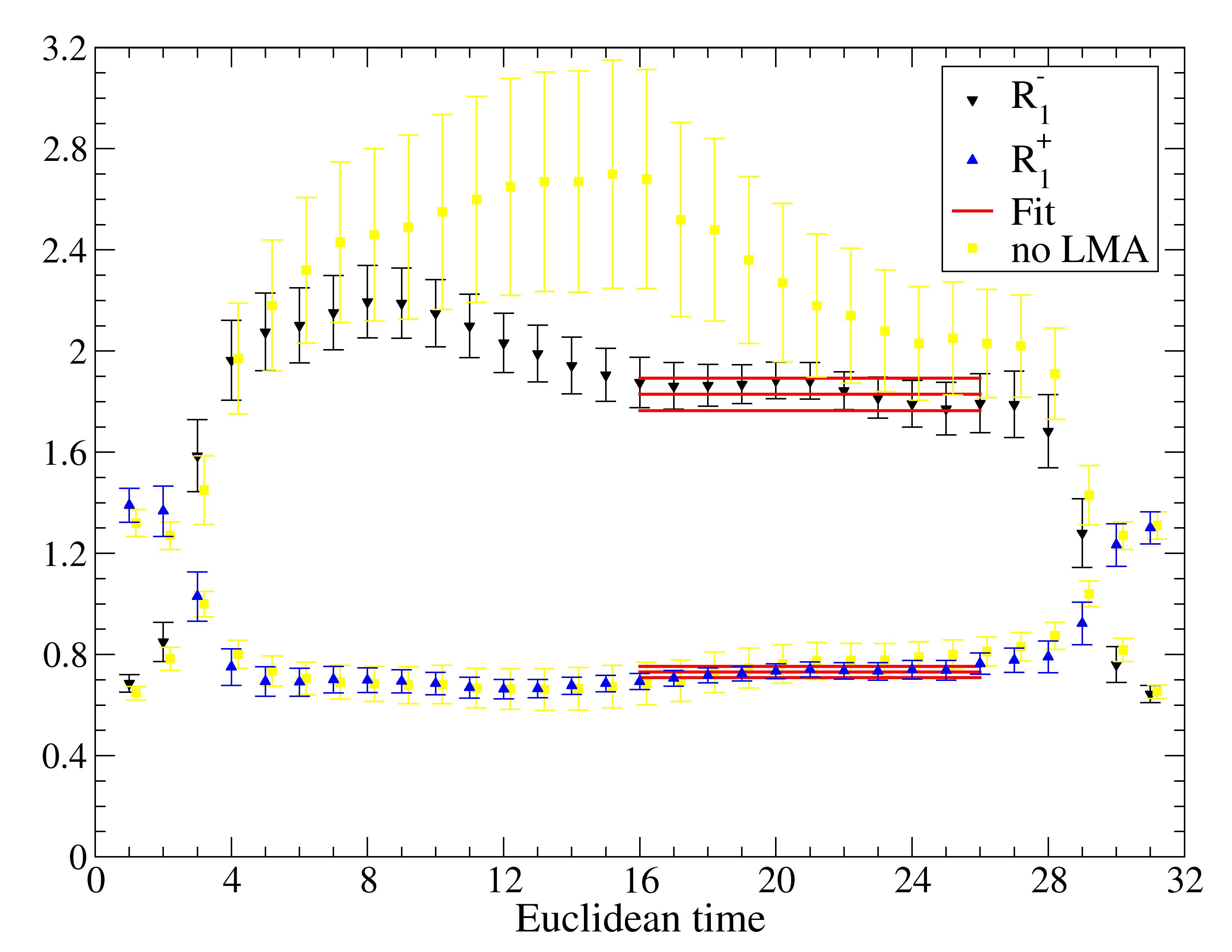
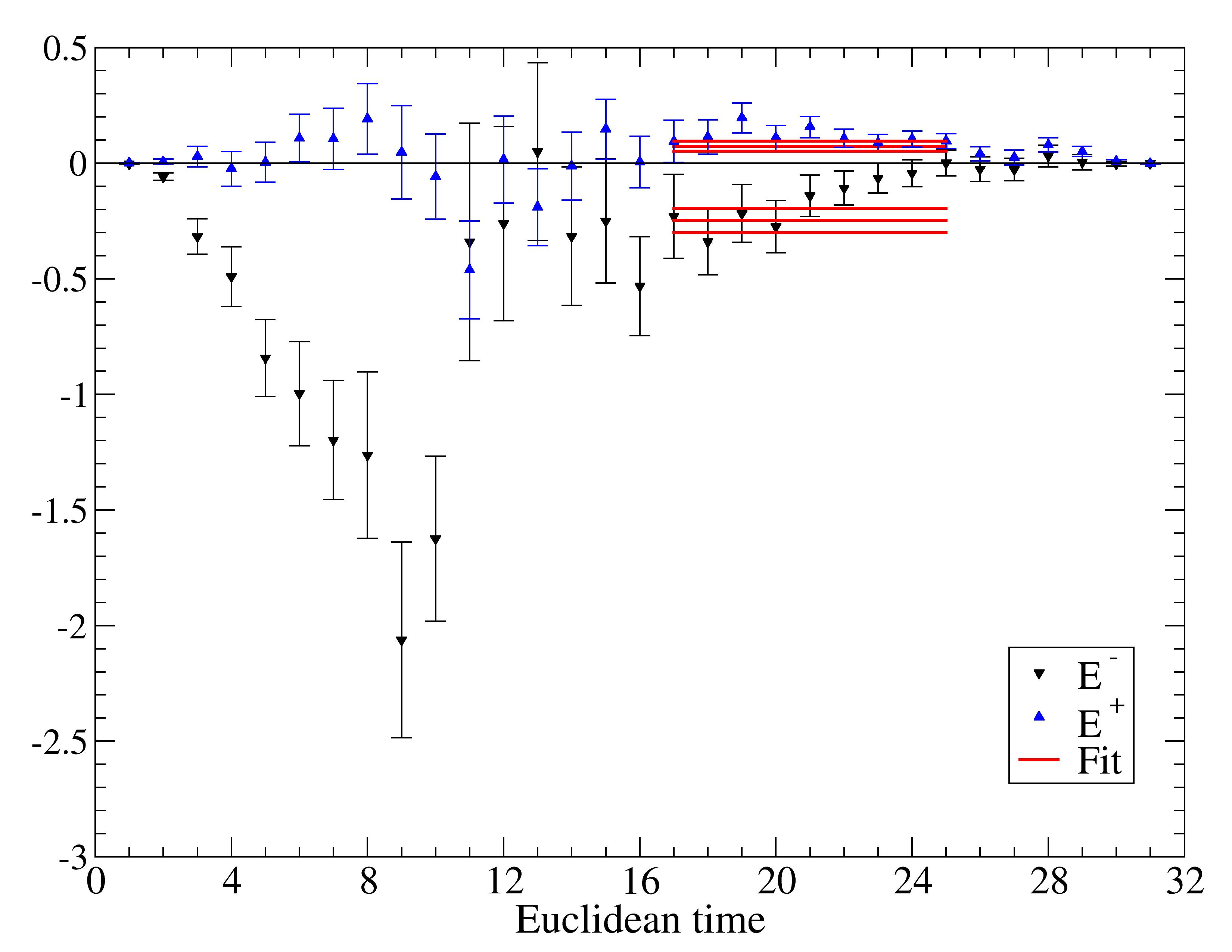
Figure 6: Left: contribution to the ratios $R_{1}^{\pm}$ coming from the eight-diagram for $am_{u}=0.03$, together with the fit to a plateau in some interval of Euclidean times. (The value of Euclidean times is shifted by $10$ lattice units with respect to the conventions in the main text.) The yellow points, corresponding to the computation that does not use low-mode averaging, illustrate the impact of the latter on the signal. Right: contribution to the ratios $R_{1}^{\pm}$ coming from the eye-diagram for $am_{u}=0.02,am_{c}=0.2$.

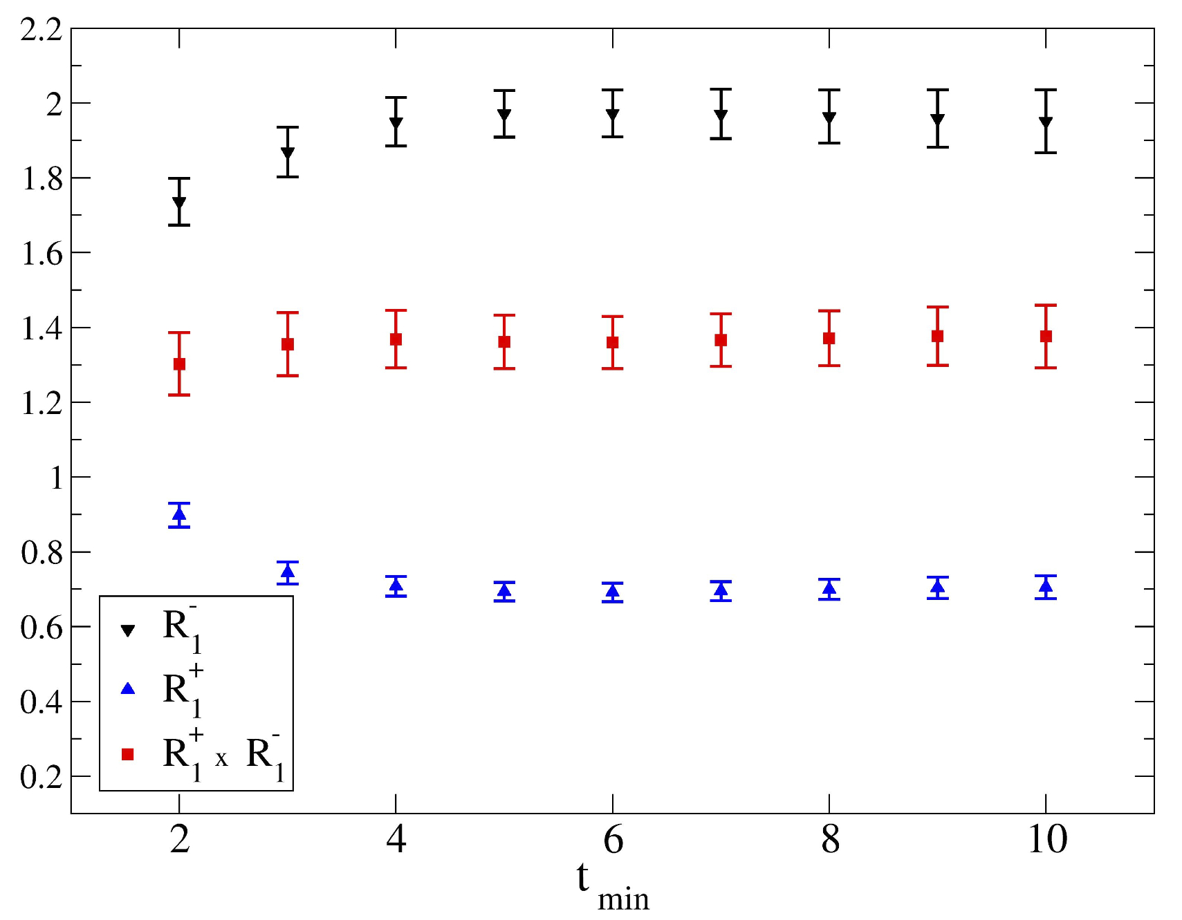
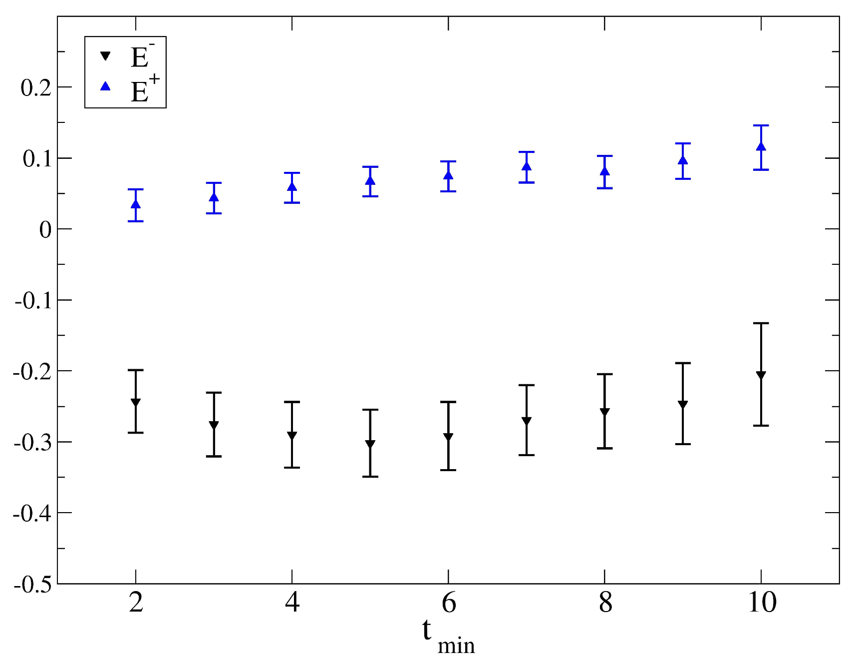
Figure 7: Left: result for the fit to the contribution to $R_{1}^{\pm}$ ($am_{u}=0.03$) coming from the eight-diagram as a function of the plateau choice, parametrised by the minimal separation (in lattice units) $t_{\rm min}$ allowed between operator insertions. The combination $R_{1}^{+}+R_{1}^{-}$ is also displayed. Right: idem for the eye-diagram ($am_{u}=0.03$, $am_{c}=0.2$).

References

- [1] M. Gaillard and B. Lee, Rule for Nonleptonic Decays in Asymptotically Free Field Theories, Phys.Rev.Lett. 33 (1974) 108.
- [2] G. Altarelli and L. Maiani, Octet Enhancement of Nonleptonic Weak Interactions in Asymptotically Free Gauge Theories, Phys.Lett. B52 (1974) 351–354.
- [3] N. Cabibbo, G. Martinelli, and R. Petronzio, Weak Interactions on the Lattice, Nucl.Phys. B244 (1984) 381–391.
- [4] R. Brower, G. Maturana, M. Gavela, and R. Gupta, Calculation of Weak Transitions in Lattice QCD, Phys.Rev.Lett. 53 (1984) 1318.
- [5] V. Cirigliano, G. Ecker, H. Neufeld, A. Pich, and J. Portoles, Kaon Decays in the Standard Model, Rev.Mod.Phys. 84 (2012) 399, [arXiv:1107.6001].
- [6] A. J. Buras, J.-M. Gerard, and W. A. Bardeen, Large N Approach to Kaon Decays and Mixing 28 Years Later: Rule, and , arXiv:1401.1385.
- [7] L. Maiani and M. Testa, Final state interactions from Euclidean correlation functions, Phys.Lett. B245 (1990) 585–590.
- [8] L. Lellouch and M. Lüscher, Weak transition matrix elements from finite volume correlation functions, Commun.Math.Phys. 219 (2001) 31–44, [hep-lat/0003023].
- [9] C. Lin, G. Martinelli, C. Sachrajda, and M. Testa, decays in a finite volume, Nucl.Phys. B619 (2001) 467–498, [hep-lat/0104006].
- [10] C. Pena, S. Sint, and A. Vladikas, Twisted mass QCD and lattice approaches to the rule, JHEP 0409 (2004) 069, [hep-lat/0405028].
- [11] R. Frezzotti and G. Rossi, Chirally improving Wilson fermions. II. Four-quark operators, JHEP 0410 (2004) 070, [hep-lat/0407002].
- [12] P. Ginsparg and K. Wilson, A Remnant of Chiral Symmetry on the Lattice, Phys.Rev. D25 (1982) 2649.
- [13] D. Kaplan, A Method for simulating chiral fermions on the lattice, Phys.Lett. B288 (1992) 342–347, [hep-lat/9206013].
- [14] D. Kaplan, Chiral fermions on the lattice, Nucl.Phys.Proc.Suppl. 30 (1993) 597–600.
- [15] Y. Shamir, Chiral fermions from lattice boundaries, Nucl.Phys. B406 (1993) 90–106, [hep-lat/9303005].
- [16] V. Furman and Y. Shamir, Axial symmetries in lattice QCD with Kaplan fermions, Nucl.Phys. B439 (1995) 54–78, [hep-lat/9405004].
- [17] P. Hasenfratz, Prospects for perfect actions, Nucl.Phys.Proc.Suppl. 63 (1998) 53–58, [hep-lat/9709110].
- [18] P. Hasenfratz, Lattice QCD without tuning, mixing and current renormalization, Nucl.Phys. B525 (1998) 401–409, [hep-lat/9802007].
- [19] H. Neuberger, Exactly massless quarks on the lattice, Phys.Lett. B417 (1998) 141–144, [hep-lat/9707022].
- [20] M. Lüscher, Exact chiral symmetry on the lattice and the Ginsparg-Wilson relation, Phys.Lett. B428 (1998) 342–345, [hep-lat/9802011].
- [21] P. Hernández, K. Jansen, and M. Lüscher, Locality properties of Neuberger’s lattice Dirac operator, Nucl.Phys. B552 (1999) 363–378, [hep-lat/9808010].
- [22] S. Capitani and L. Giusti, Analysis of the rule and with overlap fermions, Phys.Rev. D64 (2001) 014506, [hep-lat/0011070].
- [23] CP-PACS Collaboration Collaboration, J. Noaki et. al., Calculation of nonleptonic kaon decay amplitudes from matrix elements in quenched domain wall QCD, Phys.Rev. D68 (2003) 014501, [hep-lat/0108013].
- [24] RBC Collaboration Collaboration, T. Blum et. al., Kaon matrix elements and CP violation from quenched lattice QCD: 1. The three flavor case, Phys.Rev. D68 (2003) 114506, [hep-lat/0110075].
- [25] T. Blum, P. Boyle, N. Christ, N. Garron, E. Goode, et. al., to Decay amplitudes from Lattice QCD, Phys.Rev. D84 (2011) 114503, [arXiv:1106.2714].
- [26] RBC, UKQCD Collaboration, P. Boyle et. al., Emerging understanding of the Rule from Lattice QCD, Phys.Rev.Lett. 110 (2013), no. 15 152001, [arXiv:1212.1474].
- [27] M. Shifman, A. Vainshtein, and V. Zakharov, Light Quarks and the Origin of the Rule in the Nonleptonic Decays of Strange Particles, Nucl.Phys. B120 (1977) 316.
- [28] L. Giusti, P. Hernández, M. Laine, P. Weisz, and H. Wittig, A Strategy to study the role of the charm quark in explaining the rule, JHEP 0411 (2004) 016, [hep-lat/0407007].
- [29] C. Bernard, T. Draper, A. Soni, H. Politzer, and M. Wise, Application of Chiral Perturbation Theory to Decays, Phys.Rev. D32 (1985) 2343–2347.
- [30] L. Giusti, P. Hernández, M. Laine, C. Pena, J. Wennekers, and H. Wittig, On amplitudes with a light charm quark, Phys.Rev.Lett. 98 (2007) 082003, [hep-ph/0607220].
- [31] P. Hernández, M. Laine, C. Pena, E. Torró, J. Wennekers, and H. Wittig, Determination of the weak Hamiltonian in the chiral limit through topological zero-mode wave functions, JHEP 0805 (2008) 043, [arXiv:0802.3591].
- [32] E. Endress and C. Pena, Variance Reduction with Practical All-to-All Lattice Propagators, to appear.
- [33] P. Hernández and M. Laine, Probing the chiral weak Hamiltonian at finite volumes, JHEP 0610 (2006) 069, [hep-lat/0607027].
- [34] G. Altarelli, G. Curci, G. Martinelli, and S. Petrarca, QCD Nonleading Corrections to Weak Decays as an Application of Regularization by Dimensional Reduction, Nucl.Phys. B187 (1981) 461.
- [35] A. Buras and P. Weisz, QCD Nonleading Corrections to Weak Decays in Dimensional Regularization and ’t Hooft-Veltman Schemes, Nucl.Phys. B333 (1990) 66.
- [36] M. Ciuchini, E. Franco, V. Lubicz, G. Martinelli, I. Scimemi, et. al., Next-to-leading order QCD corrections to effective Hamiltonians, Nucl.Phys. B523 (1998) 501–525, [hep-ph/9711402].
- [37] A. Buras, M. Misiak, and J. Urban, Two loop QCD anomalous dimensions of flavor changing four quark operators within and beyond the standard model, Nucl.Phys. B586 (2000) 397–426, [hep-ph/0005183].
- [38] ALPHA Collaboration Collaboration, M. Guagnelli, J. Heitger, C. Pena, S. Sint, and A. Vladikas, Non-perturbative renormalization of left-left four-fermion operators in quenched lattice QCD, JHEP 0603 (2006) 088, [hep-lat/0505002].
- [39] ALPHA Collaboration Collaboration, P. Dimopoulos et. al., Non-perturbative renormalisation of Delta F=2 four-fermion operators in two-flavour QCD, JHEP 0805 (2008) 065, [arXiv:0712.2429].
- [40] P. Dimopoulos, L. Giusti, P. Hernández, F. Palombi, C. Pena, et. al., Non-perturbative renormalisation of left-left four-fermion operators with Neuberger fermions, Phys.Lett. B641 (2006) 118–124, [hep-lat/0607028].
- [41] R. Crewther, Chiral Reduction of Amplitudes, Nucl.Phys. B264 (1986) 277.
- [42] P. Hernández and M. Laine, Charm mass dependence of the weak Hamiltonian in chiral perturbation theory, JHEP 0409 (2004) 018, [hep-ph/0407086].
- [43] J. Gasser and H. Leutwyler, Thermodynamics of Chiral Symmetry, Phys.Lett. B188 (1987) 477.
- [44] J. Gasser and H. Leutwyler, Spontaneously Broken Symmetries: Effective Lagrangians at Finite Volume, Nucl.Phys. B307 (1988) 763.
- [45] H. Neuberger, A Better Way to Measure in the Linear Model, Phys.Rev.Lett. 60 (1988) 889.
- [46] H. Neuberger, Soft Pions in Large Boxes, Nucl.Phys. B300 (1988) 180.
- [47] H. Leutwyler, Energy Levels of Light Quarks Confined to a Box, Phys.Lett. B189 (1987) 197.
- [48] F. Hansen and H. Leutwyler, Charge correlations and topological susceptibility in QCD, Nucl.Phys. B350 (1991) 201–227.
- [49] J. Kambor, J. Missimer, and D. Wyler, The Chiral Loop Expansion of the Nonleptonic Weak Interactions of Mesons, Nucl.Phys. B346 (1990) 17–64.
- [50] M. Golterman and E. Pallante, Effects of quenching and partial quenching on penguin matrix elements, JHEP 0110 (2001) 037, [hep-lat/0108010].
- [51] M. Golterman and E. Pallante, On the effects of (partial) quenching on penguin contributions to , Phys.Rev. D69 (2004) 074503, [hep-lat/0212008].
- [52] M. Ademollo and R. Gatto, Nonrenormalization Theorem for the Strangeness Violating Vector Currents, Phys.Rev.Lett. 13 (1964) 264–265.
- [53] H. Neuberger, More about exactly massless quarks on the lattice, Phys.Lett. B427 (1998) 353–355, [hep-lat/9801031].
- [54] L. Giusti, C. Hoelbling, M. Lüscher, and H. Wittig, Numerical techniques for lattice QCD in the epsilon regime, Comput.Phys.Commun. 153 (2003) 31–51, [hep-lat/0212012].
- [55] P. Hasenfratz, V. Laliena, and F. Niedermayer, The Index theorem in QCD with a finite cutoff, Phys.Lett. B427 (1998) 125–131, [hep-lat/9801021].
- [56] L. Del Debbio, L. Giusti, and C. Pica, Topological susceptibility in the SU(3) gauge theory, Phys.Rev.Lett. 94 (2005) 032003, [hep-th/0407052].
- [57] S. Necco and R. Sommer, The heavy quark potential from short to intermediate distances, Nucl.Phys. B622 (2002) 328–346, [hep-lat/0108008].
- [58] J. Wennekers and H. Wittig, On the renormalized scalar density in quenched QCD, JHEP 0509 (2005) 059, [hep-lat/0507026].
- [59] L. Giusti, M. Lüscher, P. Weisz, and H. Wittig, Lattice QCD in the epsilon regime and random matrix theory, JHEP 0311 (2003) 023, [hep-lat/0309189].
- [60] T. DeGrand and S. Schaefer, Improving meson two point functions in lattice QCD, Comput.Phys.Commun. 159 (2004) 185–191, [hep-lat/0401011].
- [61] L. Giusti, P. Hernández, M. Laine, P. Weisz, and H. Wittig, Low-energy couplings of QCD from current correlators near the chiral limit, JHEP 0404 (2004) 013, [hep-lat/0402002].
- [62] L. Giusti, C. Pena, P. Hernández, M. Laine, J. Wennekers, and H. Wittig, On the determination of low-energy constants for transitions, PoS LAT2005 (2006) 344, [hep-lat/0510033].
- [63] S. Bernardson, P. McCarty, and C. Thron, Monte Carlo methods for estimating linear combinations of inverse matrix entries in lattice QCD, Comput.Phys.Commun. 78 (1993) 256–264.
- [64] S.-J. Dong and K.-F. Liu, Stochastic estimation with Z(2) noise, Phys.Lett. B328 (1994) 130–136, [hep-lat/9308015].
- [65] J. M. Tang and Y. Saad, A probing method for computing the diagonal of a matrix inverse, Numerical Linear Algebra with Applications 19 (2011), no. 3 485–501.
- [66] L. Giusti, P. Hernández, S. Necco, C. Pena, J. Wennekers, and H. Wittig, Testing chiral effective theory with quenched lattice QCD, JHEP 0805 (2008) 024, [arXiv:0803.2772].
- [67] P. Hasenfratz and H. Leutwyler, Goldstone Boson Related Finite Size Effects in Field Theory and Critical Phenomena With O() Symmetry, Nucl.Phys. B343 (1990) 241–284.
- [68] F. Hansen, Finite Size Effects in Spontaneously Broken SU() SU() Theories, Nucl.Phys. B345 (1990) 685–708.
- [69] J. Gasser and H. Leutwyler, Chiral Perturbation Theory: Expansions in the Mass of the Strange Quark, Nucl.Phys. B250 (1985) 465.
- [70] A. Bazavov, D. Toussaint, C. Bernard, J. Laiho, C. DeTar, et. al., Nonperturbative QCD simulations with 2+1 flavors of improved staggered quarks, Rev.Mod.Phys. 82 (2010) 1349–1417, [arXiv:0903.3598].
- [71] MILC Collaboration Collaboration, A. Bazavov et. al., MILC results for light pseudoscalars, PoS CD09 (2009) 007, [arXiv:0910.2966].
- [72] MILC Collaboration Collaboration, A. Bazavov et. al., Results for light pseudoscalar mesons, PoS LATTICE2010 (2010) 074, [arXiv:1012.0868].
- [73] S. Aoki et. al., Review of lattice results concerning low energy particle physics, arXiv:1310.8555.
- [74] M. E. Peskin and D. V. Schroeder, An Introduction To Quantum Field Theory (Frontiers in Physics). Westview Press, 1995.