Lifshitz Quartic Quasitopological Black Holes

Abstract

In this paper we shall elucidate some of the effects of the quartic quasitopological term for Lifshitz-symmetric black holes. The field equations of this theory are difficult to solve exactly; here we will use numerical solutions both to verify previous exact solutions for quartic quasitopological AdS black holes as well as to examine new quasitopological Lifshitz-symmetric black hole solutions, in order to determine the effect of the quartic coupling parameter on the black hole’s thermodynamic behaviour. We shall find that the quartic parameter controls solutions very similarly to the cubic parameter, allowing for the construction of a theory with another free parameter which may find meaning in the phase transition behaviour of a gauge/gravity context.

I Introduction

It is suspected that quantum gravity can be explained by a topological field theory, in the sense that all of the gravitational degrees of freedom live on the boundary field theory. This is the principle of holography; much progress in the understanding of the holographic principle has been made in recent years. The evidence for holography has been explored since 1997 when Juan Maldacena conjectured the AdS/CFT correspondence Maldacena1 ; Maldacena2 .

The AdS/CFT correspondence relates an asymptotically anti-de Sitter (AdS) bulk theory with gravity in $(n+1)$-dimensions to a conformal field theory on its $n$-dimensional Minkowski spacetime boundary at infinity. As Einstein gravity does not have enough free parameters to make a one-to-one relationship between central charges and couplings on the non-gravitational side and the “coupling” parameters on the gravitational side, one may wish to study modified theories, such as Lovelock theory Friedman1 ; Friedman2 ; Jacobson or quasitopological gravity Lemos1 ; Lemos2 ; Lemos3 ; Aminneborg ; Mann ; Cai ; Dehghani1 ; Dehghani2 ; Dehghani3 ; Brenna2012 , where higher curvature terms produce additional coupling parameters.

One could consider modifying the gravitational part of the Einstein action with higher-derivative terms which arise in additional powers of the curvature. Some gravity theories, like Lovelock gravity, play a important role on the gravity side of the duality conjecture Boera ; Camanho . The quasitopological framework is very similar to Lovelock gravity, allowing for additional coupling parameters in a given dimension, but at the cost of requiring spherical symmetry (otherwise the equations of motion become greater than second-order). The benefit to this approach is that quasitopological gravity can produce coupling terms in fewer dimensions than Lovelock gravity, due to the fact that while Lovelock terms become topological surface terms for a given number of dimensions, quasitopological terms are not true topological invariants and therefore produce nontrivial gravitational effects in fewer dimensions than the corresponding Lovelock terms. Black hole solutions in quartic quasitopological gravity are not new Ghanaatian1 ; Ghanaatian2 ; Ghanaatian3 , but the field equations generated by the quartic terms are lengthy and numerical solutions are challenging to obtain. Here we investigate asymptotically Lifshitz solutions of black holes in quartic quasitopological gravity. The following (asymptotic) form of spacetime metric is suggested from the holographically Lifshitz condensed matter theories as

$$ds^{2}=L^{2}(-r^{2z}dt^{2}+\frac{dr^{2}}{r^{2}}+r^{2}dX^{2})$$ (1)

which is based on the anisotropic scaling transformation (Lifshitz scaling)

$$t\rightarrow{\lambda}^{z}t,\text{ \ }r\rightarrow{\lambda}^{-1}r,\text{ \ }X\rightarrow\lambda X$$ (2)

This paper is organized as follows. We review the action of quartic quasitopological gravity and obtain the field equations in Section II. Section III contains the calculation of the conserved quantity along the radial coordinate $r$. In Section IV, we consider two cases: the first Lifshitz solution is obtained in the absence of matter, and then we derive the conditions on a Lifshitz solution in the presence of a massive gauge field. Section V is devoted to the calculation of the asymptotically Lifshitz black hole solutions near the horizon and at large $r$. In Section VI, we first check that new numerical solutions agree with exact solutions for $z=1$, and then we find numerical quasitopological Lifshitz-symmetric black hole solutions for $z=2$. In Section VII, by using the numerical results, we obtain the entropy and temperature of the black hole and examine the thermodynamical behavior of the black hole for $z=2$ in $3^{rd}$ and $4^{th}$ order quasitopological gravity. Finally, we finish this paper with some concluding remarks.

II The Field Equations Of Quasitopological Gravity

Here we will derive field equations from the action of quasitopological gravity up to the $4^{th}$ order. In addition, to maintaining an asymptotically Lifshitz metric, a Proca field must be introduced. The action can be written as

$$I=\int d^{n+1}x\sqrt{-g}\left(-2\Lambda+\mathcal{L}_{1}+{\mu_{2}}\mathcal{L}_{2}+{\mu_{3}}\mathcal{X}_{3}+{\mu_{4}}\mathcal{X}_{4}-\frac{1}{4}F_{\mu\nu}F^{\mu\nu}-\frac{1}{2}m^{2}A_{\mu}A^{\mu}\right)$$ (3)

where $(n+1)$ is the number of dimensions of the spacetime, $F_{\mu\nu}=\partial_{\mu}A_{\nu}-\partial_{\nu}A_{\mu}$ is the Proca field strength, $A_{\mu}$ is the Proca vector potential, $\mathcal{L}_{1}={R}$ is the Einstein-Hilbert Lagrangian, and $\mathcal{L}_{2}=R_{abcd}{R}^{abcd}-4{R}_{ab}{R}^{ab}+{R}^{2}$ is the Gauss-Bonnet Lagrangian, $\mathcal{X}_{3}$ and $\mathcal{X}_{3}$ are third and fourth order of quasitopological gravity, respectively, which can be written as (Myers2010 ; Ghanaatian1 ):

$$\mathcal{X}_{3} = R_{ab}^{cd}R_{cd}^{\,\,e\,\,\,f}R_{e\,\,f}^{\,\,a\,\,\,b}+\frac{1}{(2n-1)(n-3)}\left(\frac{3(3n-5)}{8}R_{abcd}R^{abcd}R\right.$$ (4)

$$-3(n-1)R_{abcd}R^{abc}{}_{e}R^{de}+3(n+1)R_{abcd}R^{ac}R^{bd}$$

$$\left.+\,6(n-1)R_{a}{}^{b}R_{b}{}^{c}R_{c}{}^{a}-\frac{3(3n-1)}{2}R_{a}^{\,\,b}R_{b}^{\,\,a}R+\frac{3(n+1)}{8}R^{3}\right)$$

$$\mathcal{X}_{4} = c_{1}R_{abcd}R^{cdef}R_{\phantom{hg}{ef}}^{hg}R_{hg}{}^{ab}+c_{2}R_{abcd}R^{abcd}R_{ef}R^{ef}+c_{3}RR_{ab}R^{ac}R_{c}{}^{b}+c_{4}(R_{abcd}R^{abcd})^{2}$$ (5)

$$+c_{5}R_{ab}R^{ac}R_{cd}R^{db}+c_{6}RR_{abcd}R^{ac}R^{db}+c_{7}R_{abcd}R^{ac}R^{be}R_{\phantom{d}{e}}^{d}+c_{8}R_{abcd}R^{acef}R_{\phantom{b}{e}}^{b}R_{\phantom{d}{f}}^{d}$$

$$+c_{9}R_{abcd}R^{ac}R_{ef}R^{bedf}+c_{10}R^{4}+c_{11}R^{2}R_{abcd}R^{abcd}+c_{12}R^{2}R_{ab}R^{ab}$$

$$+c_{13}R_{abcd}R^{abef}R_{ef}{}_{g}^{c}R^{dg}+c_{14}R_{abcd}R^{aecf}R_{gehf}R^{gbhd},$$

where the $c_{i}$ (quasitopological fixed constants) have dimensional dependence and are tuned as per Myers2010 to produce a simplification of the action (seen below in equation 9). See Ghanaatian1 (equation (7)) for the detailed values used here.

Note that $\mathcal{X}_{3}$ and $\mathcal{X}_{4}$ are only effective in dimensions greater than four and they become trivial in six and eight dimensions respectively (Refs. Myers2010 ; Ghanaatian1 ). We use the asymptotically Lifshitz metric in the spherically symmetric case as follows:

$$ds^{2}=-\frac{r^{2z}}{L^{2z}}f(r)dt^{2}+\frac{L^{2}dr^{2}}{r^{2}g(r)}+r^{2}d\Omega^{2}$$ (6)

where boundary conditions require that $f(r)$ and $g(r)$ must go to 1 as $r$ goes to infinity. The term $d\Omega^{2}$ is the metric of an $n+1$ dimensional hypersurface with constant curvature $(n-1)(n-2)k$ and volume $V_{n-1}$

$$d\Omega^{2}=d{\theta_{1}}^{2}+k^{-1}\sin^{2}{\left(\sqrt{k}\theta_{1}\right)}\left(d{\theta_{2}}^{2}+\displaystyle\sum\limits_{i=3}^{D-2}\displaystyle\prod\limits_{j=2}^{i-1}\sin^{2}{\theta_{j}}d{\theta_{i}}^{2}\right)$$ (7)

where the parameter $k$ specifies hyperbolic, flat, and spherical geometries with the values $-1$, $0$, or $1$, respectively. For $k=0$ a coordinate transformation will reduce this portion of the metric to the form $\sum_{k}^{D-2}d{\theta_{k}}^{2}$. To match the spherical symmetry, we use a radial gauge field ansatz; for simplicity we extract the $r^{z}$ dependence and write it as

$$A_{t}=q\frac{r^{z}}{L^{z}}h(r).$$ (8)

where $h(r)$ also tends to unity at $r\rightarrow\infty$.

Because we seek solutions in the context of a gauge/gravity duality, we will examine a five dimensional gravity theory for applicability to a four dimensional gauge theory. Under these considerations, one can obtain the effective action for the spherically symmetric case as:

$$I = \int d^{4}x\int dr\frac{r^{z-1}}{kL^{z+1}}\sqrt{\frac{f}{g}}\left(\left\{3r^{4}\left(\frac{-\Lambda}{6}L^{2}-\Psi+\hat{\mu_{2}}\Psi^{2}+\hat{\mu_{3}}\Psi^{3}+\hat{\mu_{4}}\Psi^{4}\right)\right\}^{\prime}\right.$$ (9)

$$\left.+\frac{q^{2}r^{3}}{2f}\left(g\left(rh^{\prime}+zh\right)^{2}+m^{2}L^{2}h^{2}\right)\right)$$

where $\Psi=\left(g-\frac{L^{2}}{r^{2}}k\right)$ and the dimensionless parameters $\hat{\mu}_{2}$, $\hat{\mu}_{3}$ and $\hat{\mu}_{4}$ are redefinitions of the dimensionless coupling constants (to produce an action that is cleaner to vary):

$$\hat{\mu}_{2}\equiv\frac{(n-2)(n-3)}{l^{2}}\mu_{2},\text{ \ \ \ }\hat{\mu}_{3}\equiv-\frac{(n-2)(n-5)(3n^{2}-9n+4)}{8(2n-1)l^{4}}\mu_{3},$$

$$\hat{\mu}_{4}\equiv{\frac{n\left(n-1\right)\left(n-2\right)^{2}\left(n-3\right)\left(n-7\right)({{n}^{5}-15\,{n}^{4}+72\,{n}^{3}-156\,{n}^{2}+150\,n-42)}}{{l}^{6}}}\mu_{4},$$

Varying the action of equation (9) with respect $g(r)$, $f(r)$, and $h(r)$ respectively yields the following equations of motion:

$$\Lambda L^{2}r^{8}+6\hat{\mu_{4}}\left(1-2z\right)g^{4}r^{8}+\left(3z+3\right)r^{8}g-6z\hat{\mu_{2}}r^{8}g^{2}+12\hat{\mu_{4}}L^{2}k\left(3z-2\right)g^{3}r^{6}+6z\hat{\mu_{2}}r^{6}L^{2}kg$$

$$-3r^{6}L^{2}k-\left(9z-3\right)\hat{\mu_{3}}r^{8}g^{3}+\left(18z-9\right)\hat{\mu_{3}}r^{6}L^{2}kg^{2}+36\hat{\mu_{4}}L^{4}k^{2}\left(1-z\right)r^{4}-\left(9z-9\right)\hat{\mu_{3}}L^{4}k^{2}r^{4}g$$

$$+12\hat{\mu_{4}}L^{6}k\left(z-2\right)gr^{2}-3\hat{\mu_{3}}L^{6}k^{3}r^{2}+6\hat{\mu_{4}}L^{8}k^{2}+g(\ln{f})^{{}^{\prime}}\left(\frac{3}{2}r^{9}-3\right.\hat{\mu_{2}}r^{9}g+3\hat{\mu_{2}}r^{7}L^{2}k$$

$$-\frac{9}{2}\hat{\mu_{3}}r^{9}g^{2}+\left.9\hat{\mu_{3}}r^{7}gL^{2}k-\frac{9}{2}\hat{\mu_{3}}r^{5}L^{4}k^{2}-6\hat{\mu_{4}}g^{3}r^{9}+18\hat{\mu_{4}}L62kg^{2}r^{7}-18\hat{\mu_{4}}L^{4}k^{2}gr^{5}+6\hat{\mu_{4}}r^{3}L^{6}k\right)$$

$$\quad\quad\quad\quad=\frac{q^{2}r^{8}}{4f}\left[g\left(rh^{{}^{\prime}}+zh\right)^{2}-m^{2}L^{2}h^{2}\right]$$ (10)

$$\left(3r^{4}\left[-\frac{\Lambda}{6}L^{2}-\Psi+\hat{\mu_{2}}\Psi^{2}+\hat{\mu_{3}}\Psi^{3}+\hat{\mu_{4}}\Psi^{4}\right]\right)^{\prime}=\frac{q^{2}r^{3}}{2f}\left[g\left(rh^{{}^{\prime}}+zh\right)^{2}+m^{2}L^{2}h^{2}\right]$$ (11)

$$2r^{2}h^{\prime\prime}-r\left[(\ln f)^{\prime}-(\ln g)^{\prime}\right](rh^{\prime}+zh)+2(z+4)rh^{\prime}+6zh=2m^{2}L^{2}\frac{h}{g}$$ (12)

where a prime (^′) represents the derivative with respect to the radial coordinate $r$.

III The Conserved Quantity

In order to calculate the conserved quantity along the radial coordinate $r$, we calculate the first integral of the equations of motion. Since there is no exact quasitopological-Lifshitz solution, we can evaluate the conserved quantity at $r=\infty$ and at the horizon in order to obtain it explicitly.

It is simpler if we redefine the metric using a different ansatz, as in Dehghani2010 .

$$F(r) =\frac{1}{2}\ln{f(r)}+z\ln{\frac{r}{L}},$$

$$G(r) =-\frac{1}{2}\ln{g(r)}-\ln{\frac{r}{L}},$$

$$R(r) =\ln{\frac{r}{L}},$$

$$H(r) =\ln{h(r)}+z\ln{\frac{r}{L}},$$ (13)

the metric may be written as:

$$ds^{2}=-e^{2F(r)}dt^{2}+e^{2G(r)}dr^{2}+e^{2R(r)}\frac{1}{L^{2}}d\Omega^{2}$$ (14)

One can reduce the action to one dimension and obtain the equation of motion. We insert this into the action (9); after integrating by parts we obtain a one dimensional Lagrangian $\mathcal{L}_{1D}=\mathcal{L}_{1g}+\mathcal{L}_{1m}$ where

$$\mathcal{L}_{1g} =(n-1)\left(-2\frac{\hat{\mu_{2}}}{n-1}e^{2G}+\left[2F^{{}^{\prime}}R^{{}^{\prime}}+(n-1)R^{\prime 2}\right]\right.$$

$$-\frac{\hat{\mu_{2}}L^{2}}{3}\left[4F^{\prime}R^{\prime 3}+(n-4)R^{\prime 4}\right]e^{-2G}$$

$$\quad-\left.\vphantom{\frac{\hat{\mu_{2}}}{n-1}}\frac{\hat{\mu_{3}}}{5}L^{4}\left[6F^{\prime}R^{\prime 5}+(n-6)R^{\prime 6}\right]e^{-4G}\right.$$

$$\left.-\frac{\hat{\mu_{{4}}}}{7}{L}^{6}{e^{-6\,G}}\left(8\,{\it F^{{}^{\prime}}}\,{{\it R^{{}^{\prime}}}}^{7}+\left(n-8\right){{\it R^{{}^{\prime}}}}^{8}\right)\right)e^{F-G+(n-1)R}$$ (15)

$$\mathcal{L}_{1m} =\frac{1}{2}q^{2}\left(m^{2}+H^{\prime 2}e^{-2G}\right)e^{-F+G+(n-1)R+2H}.$$ (16)

Calculating the equations of motion from the above action, we have:

$$\mathcal{L}_{1g}-\mathcal{L}_{1m}=\left\{2\left(n-1\right){e^{F-G+\left(n-2\right)R}}\right. \left.\left(\,{\it R^{{}^{\prime}}}-\frac{2}{3}\,\hat{\mu_{{2}}}{l}^{2}{e^{-2\,G}}{{\it R^{{}^{\prime}}}}^{3}\right.\right.$$

$$\left.\left.-\frac{3}{5}\,\hat{\mu_{{3}}}{l}^{4}{e^{-4\,G}}{{\it R^{{}^{\prime}}}}^{5}-{\frac{4}{7}}\,\hat{\mu_{{4}}}{l}^{6}{e^{-6\,G}}{{\it R^{{}^{\prime}}}}^{7}\right)\right\}^{{}^{\prime}}$$ (17)

$$\mathcal{L}_{1g}+\mathcal{L}_{1m}=\left\{{e^{F-G+\left(n-1\right)R}}\right. \left.\left(2\,{\it F^{{}^{\prime}}}+2\,\left(n-1\right){\it R^{{}^{\prime}}}-\frac{1}{3}\,\mu_{{2}}{l}^{2}{e^{-2\,G}}\left(12\,{\it F^{{}^{\prime}}}\,{{\it R^{{}^{\prime}}}}^{2}+4\,\left(n-4\right){{\it R^{{}^{\prime}}}}^{3}\right)\right.\right.$$

$$\left.\left.-\frac{1}{5}\,\mu_{{3}}{l}^{4}{e^{-4\,G}}\left(30\,{\it F^{{}^{\prime}}}\,{{\it R^{{}^{\prime}}}}^{4}+6\,\left(n-6\right){{\it R^{{}^{\prime}}}}^{5}\right)\right.\right.$$

$$\left.\left.-\frac{1}{7}\,\mu_{{4}}{l}^{6}{e^{-6\,G}}\left(56\,{\it F^{{}^{\prime}}}\,{{\it R^{{}^{\prime}}}}^{6}+8\,\left(n-8\right){{\it R^{{}^{\prime}}}}^{7}\right)\right)\right\}^{{}^{\prime}}$$ (18)

$$2\mathcal{L}_{1m} =\left\{{q}^{2}{\it H^{{}^{\prime}}}\,{e^{-F-G+\left(n-1\right)R+2\,H}}\right\}^{{}^{\prime}}$$ (19)

We are able to obtain the conserved quantity by subtracting the sum of Eq. (III) and Eq. (III) from Eq. (19) (obtaining a total derivative) and integrating:

$$\mathcal{C}_{0} =2\left(F^{\prime}-R^{\prime}\right)\left(1-2\hat{\mu_{2}}L^{2}R^{\prime 2}e^{-2G}-3\hat{\mu_{3}}L^{4}R^{\prime 4}e^{-4G}-4\hat{\mu_{4}}L^{6}R^{\prime 6}e^{-6G}\right)e^{F-G+(n-1)R}$$

$$\quad-q^{2}H^{\prime}e^{-F-G+(n-1)R+2H}$$

$$=\left[\left(1-2\hat{\mu_{2}}g-3\hat{\mu_{3}}g^{2}-4\hat{\mu_{4}}g^{3}\right)\left(rf^{\prime}+2\left(z-1\right)f\right)-q^{2}\left(zh+rh^{\prime}\right)h\right]\frac{r^{z+n-1}}{L^{z+1}}\left(\frac{f}{g}\right)^{1/2}$$ (20)

Note that for $z=1$, where $f(r)=g(r)$, the conserved quantity reduces to

$$\mathcal{C}_{0}=\frac{r^{n+1}}{L^{2}}\left(f-\hat{\mu_{2}}f^{2}-\hat{\mu_{3}}f^{3}-\hat{\mu_{4}}f^{4}\right)^{\prime}$$

which is known to be constant in fourth order quasitopological gravity and it is proportional to the mass of the black hole.

IV Lifshitz Solutions

IV.1 Matter-free Solutions

In quasitopological gravity in the absence of matter, by setting $h(r)=0$, in 5 dimensions we investigate the solutions of the form

$$ds^{2}=-\frac{r^{2z}}{L^{2z}}dt^{2}+\frac{L^{2}dr^{2}}{r^{2}}+r^{2}\sum\limits_{i=1}^{3}d\theta_{i}^{2},$$ (21)

where $k=0$. In order to obtain an asymptotically Lifshitz solution in fourth order quasitopological gravity, the following constraints arise, for an arbitrary value of z:

$$\Lambda=-\frac{2}{{L}^{2}}({\hat{\mu_{{4}}}+2-\hat{\mu_{{2}}}}),\hskip 14.22636pt\hat{\mu_{3}}=-\frac{1}{3}(4\hat{\mu_{{4}}}-1+2\hat{\mu_{{2}}}),$$ (22)

Inserting $\hat{\mu_{3}}=\hat{\mu_{4}}=0$, these constraints reduce to those of five dimensional Gauss-Bonnet gravity Dehghani2010

$$\Lambda=-\frac{3}{L^{2}}\text{ \ \ and \ \ }\hat{\mu_{2}}=\frac{1}{2}$$ (23)

.

Note that with the above constraints, the exact Lifshitz solution (that is, $f(r)=g(r)=1$) is a solution of the field equations for any value of $z$. Inserting the conditions (22) into Eq. (11), we have

$$2-\hat{\mu_{2}}+\hat{\mu_{4}}-3\Psi+3\hat{\mu_{2}}\Psi^{2}+(1-2\hat{\mu_{2}}-4\hat{\mu_{4}})\Psi^{3}+3\hat{\mu_{4}}\Psi^{4}=\frac{C}{r^{4}}$$ (24)

where $C$ is a constant of integration. For $C=0$ ($\Psi=1$), one can obtain the following result:

$$g(r)=1+\frac{kL^{2}}{r^{2}}$$ (25)

Choosing $f(r)=g(r)$ for $k=-1$ yields an event horizon, therefore the metric

$$ds^{2}=-\frac{r^{2z}}{L^{2z}}\left(1-\frac{L^{2}}{r^{2}}\right)dt^{2}+\frac{L^{2}dr^{2}}{r^{2}(1-\frac{L^{2}}{r^{2}})}+r^{2}d\Omega_{-1}^{2}$$ (26)

is an exact black hole solution, precisely as was found in Brenna2011 .

For $z=1$, one can extend the solution found in Brenna2011 . Choosing $f(r)=g(r)$, $h(r)=0$, the field equation (12) disappears, and the equations (10) and (11) can be analytically solved. The real general solutions in $(n+1)$ dimensions of Eq. (11) are

$$f(r)=k+\frac{r^{2}}{l^{2}}\left(\frac{\hat{\mu}_{3}}{4\hat{\mu}_{4}}+\frac{1}{2}R\pm\frac{1}{2}E\right).$$ (27)

where

$$R = \left(\frac{{\hat{\mu}_{3}}^{2}}{4{\hat{\mu}_{4}}^{2}}-\frac{2\hat{\mu}_{2}}{3\hat{\mu}_{4}}+\left({\frac{D}{2}+\sqrt{\Delta}}\right)^{1/3}+\left({\frac{D}{2}-\sqrt{\Delta}}\right)^{1/3}\right)^{1/2},$$ (28)

$$E = \left(\frac{3{\hat{\mu}_{3}}^{2}}{4{\hat{\mu}_{4}}^{2}}-\frac{2\hat{\mu}_{2}}{\hat{\mu}_{4}}-R^{2}-\frac{1}{4R}\left[\frac{4\hat{\mu}_{2}\hat{\mu}_{3}}{{\hat{\mu}_{4}}^{2}}-\frac{8}{\hat{\mu}_{4}}-\frac{{\hat{\mu}_{3}}^{3}}{{\hat{\mu}_{4}}^{3}}\right]\right)^{1/2}$$ (29)

and

$$\Delta=\frac{C^{3}}{27}+\frac{D^{2}}{4}$$

$$C={\frac{3\hat{\mu}_{3}-{\hat{\mu}_{2}}^{2}}{3{\hat{\mu}_{4}}^{2}}}-\,{\frac{4\kappa}{\hat{\mu}_{4}}}$$ (30)

$$D={\frac{2}{27}}\,{\frac{{\hat{\mu}_{2}}^{3}}{{\hat{\mu}_{4}}^{3}}}-\frac{1}{3}\,\left({\frac{\hat{\mu}_{3}}{{\hat{\mu}_{4}}^{2}}}+8\,{\frac{\kappa}{\hat{\mu}_{4}}}\right)\frac{\hat{\mu}_{2}}{\hat{\mu}_{4}}+{\frac{{\hat{\mu}_{3}}^{2}\kappa}{{\hat{\mu}_{4}}^{3}}}+\frac{1}{{\hat{\mu}_{4}}^{2}}$$ (31)

and

$$\kappa=-\frac{2\Lambda}{n(n-1)}L^{2}-\frac{m}{r^{n}},$$ (32)

Note that $m$ is an integration constant.

IV.2 Matter solutions

In this section we consider another case: Lifshitz solutions in the presence of a massive gauge field $A^{\mu}$. Setting $h(r)\neq 0$ the Lifshitz solution (21) can be asymptotically obtained by using the following constraints

$$q^{2} =\frac{2\left(z-1\right)\left(1-2\hat{\mu_{2}}-3\hat{\mu_{3}}-4\hat{\mu_{4}}\right)}{z}$$ (33)

$$m^{2} =\frac{(n-1)z}{L^{2}}$$ (34)

$$\Lambda =-\frac{1}{2L^{2}}\left[(1-2\hat{\mu_{2}}-3\hat{\mu_{3}}-4\hat{\mu_{4}})\right.$$

$$\hskip 42.67912pt\left.((z-1)^{2}+n(z-2)+n^{2})+n(n-1)(\hat{\mu_{2}}+2\hat{\mu_{3}}+3\hat{\mu_{4}})\right]$$ (35)

$$\hat{\mu_{2}} <\frac{1}{2}(1-3\hat{\mu_{3}}-4\hat{\mu_{4}})$$ (36)

where the last constraint arises because we require $q^{2}>0$. This yields

$$-\frac{1}{2L^{2}}\left[(1-3\hat{\mu_{3}}\right. -4\hat{\mu_{4}})((z-1)^{2}+n(z-2)+n^{2})$$

$$\left.+n(n-1)(2\hat{\mu_{3}}+3\hat{\mu_{4}})\right] \leq\Lambda\leq-\frac{1}{4L^{2}}[n(n-1)(1+\hat{\mu_{3}}+2\hat{\mu_{4}})]$$ (37)

In the Lifshitz metrics where $z>1$, we are unable to find exact solutions so we use numerical methods.

V Asymptotically Lifshitz Black Holes

In this section, we search for asymptotically Lifshitz black hole solutions near the horizon and at large $r$. The general numeric procedure will be to construct a series solution near the horizon in order to form boundary conditions for the numerical solver. Then, the field equations (our set of nonlinear ODEs in $f(r),g(r),h(r)$) are solved numerically such that they also agree with the Lifshitz asymptotics at large $r$. This is done by iteratively solving the ODEs using the free parameters in the series solution (for $z=1$ there are two free parameters, $h_{1}$ and $f_{1}$) until the solutions converge to unity, within some tolerance (typically we set the tolerance to $10^{-8}$).

V.1 Series Solutions Near The Horizon In 5 Dimensions

Requiring that the solutions $f(r)$ and $g(r)$ tend to zero linearly near the horizon $r=r_{0}$, we write a near-horizon series expansion as

$$f(r) =f_{1}\left\{(r-r_{0})+f_{2}(r-r_{0})^{2}+f_{3}(r-r_{0})^{3}+...\right\},$$

$$g(r) =g_{1}(r-r_{0})+g_{2}(r-r_{0})^{2}+g_{3}(r-r_{0})^{3}+...,$$ (38)

$$h(r) =f_{1}^{1/2}\left\{h_{0}+h_{1}(r-r_{0})+h_{2}(r-r_{0})^{2}+h_{3}(r-r_{0})^{3}+...\right\},$$

Inserting the ansatz into the equations of the motion, we find $h_{0}=0$ and the following restriction on $g_{1}$:

$$g_{1} =\frac{z}{r_{0}^{3}}\left\{\left(\left(4\,{z}^{2}+8\,z\right){{\it r_{0}}}^{8}+12\,{l}^{8}{k}^{4}\right)\hat{\mu_{{4}}}+\left(\left(3\,{z}^{2}+6\,z+3\right){{\it r_{0}}}^{8}-6\,{l}^{6}{k}^{3}{{\it r_{0}}}^{2}\right)\hat{\mu_{{3}}}\right.$$

$$\left.+\left(2\,{z}^{2}+4\,z+6\right){{\it r_{0}}}^{8}\hat{\mu_{{2}}}+\left(-{z}^{2}-9-2\,z\right){{\it r_{0}}}^{8}-6\,{l}^{2}k{{\it r_{0}}}^{6}\right\}$$

$$\left\{\left(\left(-4\,z{{\it h_{1}}}^{2}+4\,{{\it h_{1}}}^{2}\right){{\it r_{0}}}^{7}+12\,z{l}^{6}{k}^{3}\right)\hat{\mu_{{4}}}+\left(\left(-3\,z{{\it h_{1}}}^{2}+3\,{{\it h_{1}}}^{2}\right){{\it r_{0}}}^{7}-9\,{l}^{4}{k}^{2}{{\it r_{0}}}^{2}z\right)\hat{\mu_{{3}}}\right.$$

$$\left.+\left(\left(-2\,z{{\it h_{1}}}^{2}+2\,{{\it h_{1}}}^{2}\right){{\it r_{0}}}^{7}+6\,{l}^{2}k{{\it r_{0}}}^{4}z\right)\hat{\mu_{{2}}}+\left(z{{\it h_{1}}}^{2}-{{\it h_{1}}}^{2}\right){{\it r_{0}}}^{7}+3\,{{\it r_{0}}}^{6}z\right\}^{-1}$$ (39)

where higher order expansion terms can also be written in terms of just $f_{1},h_{1}$, for example,

$$g_{2} =-{{\it r_{0}}}^{2}\left\{(((24\,\hat{\mu_{{3}}}+32\,\hat{\mu_{{4}}}+16\,\hat{\mu_{{2}}}-8){\it g_{1}}\,{{\it h_{1}}}^{2}-6\,\hat{\mu_{{2}}}{{\it g_{1}}}^{2})z\right.$$

$$+(8-32\,\hat{\mu_{{4}}}-16\,\hat{\mu_{{2}}}-24\,\hat{\mu_{{3}}}){\it g_{1}}\,{{\it h_{1}}}^{2}){{\it r_{0}}}^{7}+(((-3+6\,\hat{\mu_{{2}}}+12\,\hat{\mu_{{4}}}+9\,\hat{\mu_{{3}}}){{\it h_{1}}}^{2}+12\,{\it g_{1}}){z}^{2}$$

$$+(-6\,\hat{\mu_{{2}}}-9\,\hat{\mu_{{3}}}-12\,\hat{\mu_{{4}}}+3){{\it h_{1}}}^{2}z){{\it r_{0}}}^{6}+18\,{{\it r_{0}}}^{5}{{\it g_{1}}}^{2}z\hat{\mu_{{3}}}{l}^{2}k+(24\,{\it g_{1}}\,{z}^{2}\hat{\mu_{{2}}}{l}^{2}k-12\,z\hat{\mu_{{2}}}{l}^{2}k{\it g_{1}}){{\it r_{0}}}^{4}$$

$$\left.-36\,{{\it r_{0}}}^{3}{{\it g_{1}}}^{2}z\hat{\mu_{{4}}}{l}^{4}{k}^{2}+(36\,{\it g_{1}}\,z\hat{\mu_{{3}}}{l}^{4}{k}^{2}-36\,{\it g_{1}}\,{z}^{2}\hat{\mu_{{3}}}{l}^{4}{k}^{2}){{\it r_{0}}}^{2}+48\,{\it g_{1}}\,{z}^{2}\hat{\mu_{{4}}}{l}^{6}{k}^{3}-72\,{\it g_{1}}\,z\hat{\mu_{{4}}}{l}^{6}{k}^{3}\right\}$$

$$\left.[((1-2\,\hat{\mu_{{2}}}-3\,\hat{\mu_{{3}}}-4\,\hat{\mu_{{4}}}){\it g_{1}}\,{{\it h_{1}}}^{2}z+(-1+2\,\hat{\mu_{{2}}}+3\,\hat{\mu_{{3}}}+4\,\hat{\mu_{{4}}}){\it g_{1}}\,{{\it h_{1}}}^{2}){{\it r_{0}}}^{10}+9\,{{\it r_{0}}}^{9}z{\it g_{1}}\right.$$

$$+((-1+2\,\hat{\mu_{{2}}}+3\,\hat{\mu_{{3}}}+4\,\hat{\mu_{{4}}}){z}^{3}+(8\,\hat{\mu_{{4}}}-2+4\,\hat{\mu_{{2}}}+6\,\hat{\mu_{{3}}}){z}^{2}+(3\,\hat{\mu_{{3}}}-9+6\,\hat{\mu_{{2}}})z){{\it r_{0}}}^{8}$$

$$\left.+18\,z\hat{\mu_{{2}}}{l}^{2}k{{\it r_{0}}}^{7}{\it g_{1}}-6\,z{l}^{2}k{{\it r_{0}}}^{6}-27\,z\hat{\mu_{{3}}}{l}^{4}{k}^{2}{{\it r_{0}}}^{5}{\it g_{1}}+36\,z\hat{\mu_{{4}}}{l}^{6}{k}^{3}{{\it r_{0}}}^{3}{\it g_{1}}-6\,z\hat{\mu_{{3}}}{{\it r_{0}}}^{2}{l}^{6}{k}^{3}+12\,z\hat{\mu_{{4}}}{l}^{8}{k}^{4}\right]^{-1}$$ (40)

From this method, we find that $h_{1}$ and $f_{1}$ are both free parameters and should be chosen suitably to ensure proper asymptotic behaviour for large $r$. We can derive the remaining coefficients of the near horizon series solution up to third order in terms of these free parameters.

What we find, consistent with the third-order quasitopological case Brenna2011 , is that in $z=1$, both parameters $h_{1}$ and $f_{1}$ must be tuned to guarantee the correct asymptotic behaviour. However, in Lifshitz spacetimes, such as for $z=2$, there are numerous values of $h_{1}$ which furnish a family of black hole solutions. Furthermore, a similar approach to Brenna2011 yields the existence of a valid large-$r$ series. Therefore, solutions can have both a valid near-horizon and far-horizon expansion.

VI Numerical Solutions

VI.1 Consistency Check

We begin the numerical procedure by ensuring that our solutions agree with previous results. Due to the fact that the Lifshitz metric simplifies to AdS when $z=1$, we attempted to replicate the exact solution from Ghanaatian1 , specified in their equation (21). Because their solution was not tuned to converge to unity at infinity, we need to adjust the form of $\hat{\mu}_{0}$. Using equation (27), and the fact that our definition of $\hat{\mu}_{3}$ is equal to the negative value of their definition, this amounts to comparing our numerical solution to the exact solution

$$f(r)=k+\frac{3}{2\hat{\mu}_{2}}\frac{r^{2}}{l^{2}}\left(1-\left(1-\frac{8\hat{\mu}_{2}}{3}\left[\hat{\mu}_{0}-\frac{m}{r^{4}}\right]\right)^{1/4}\right)$$ (41)

where we have the additional conditions

$$\hat{\mu}_{0} =\frac{1}{2}\left((1-2\hat{\mu_{2}}+3\hat{\mu_{3}}-4\hat{\mu_{4}})\right.$$

$$\left.\left((z-1)^{2}+4(z-2)+16)+12(\hat{\mu_{2}}-2\hat{\mu_{3}}+3\hat{\mu_{4}})\right)\right)$$

$$\hat{\mu}_{3} =-\frac{4\hat{\mu}_{2}^{2}}{9}$$

$$\hat{\mu}_{4} =\frac{2\hat{\mu}_{2}^{3}}{27}$$

and have specified $l=1$. Note that in their metric, the $r^{2z}=r^{2}$ was absorbed into the definition of $f(r)$, so we had to multiply our results by $r^{2}$. The geometric mass $m$ controls where the event horizon is located in the analytic solution; we varied $m$ until it matched the value of the root we chose: $r_{+}=0.7$. This corresponds to $m=0.9165$. We plot the comparison for a value of $\hat{\mu}_{2}=0.2$ in figure 1.

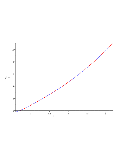
Figure 1: The overlay plot of $f(r)$ versus $r$ for the analytic solution (blue, dashed) and the numeric solution (red, dotted). Here, $\hat{\mu}_{2}=0.2$, $r_{+}=0.7$, $z=1$. The other parameters were $\hat{\mu}_{0}=0.817185,\hat{\mu}_{3}=-0.01778,\hat{\mu}_{4}=0.000593,m=0.9165$.

VI.2 Behaviour of $f(r)$

Now that we have ensured accuracy of our results as compared to the exact solutions, we are able to explore the effect of different values of $z$ on the solutions. As an example, we examine the case where $z=2$, using the parameters $\hat{\mu}_{2}=0.2,\hat{\mu}_{3}=-0.001,\hat{\mu}_{4}=0.0005,r_{+}=0.59$, where $k=1$ and the seed value for $h_{0}$ was 2.5. This is plotted in figure 2.

As we can see, a negative $3^{rd}$-order quasitopological parameter makes the peak of $f(r)$ heightened, while a positive $4^{th}$-order quasitopological parameter acts in the same manner as the $3^{rd}$-order parameter.

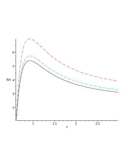
Figure 2: The plot of $f(r)$ versus $r$ for the different solutions in Gauss-Bonnet (blue, solid), $3^{rd}$-order quasitopological gravity (green, dashed), and $4^{th}$-order quasitopological gravity (red, dot-dash). Here, $r_{+}=0.59$, $k=1$, and $z=2$. The other parameters were $\hat{\mu}_{2}=0.2,\hat{\mu}_{3}=-0.001,\hat{\mu}_{4}=0.0005$.

We can explore the effect of the hypersurface curvature on the solutions of $f(r)$ by plotting a quasitopological numerical solution for values of $k=1,0,-1$. We do this in figure 3.

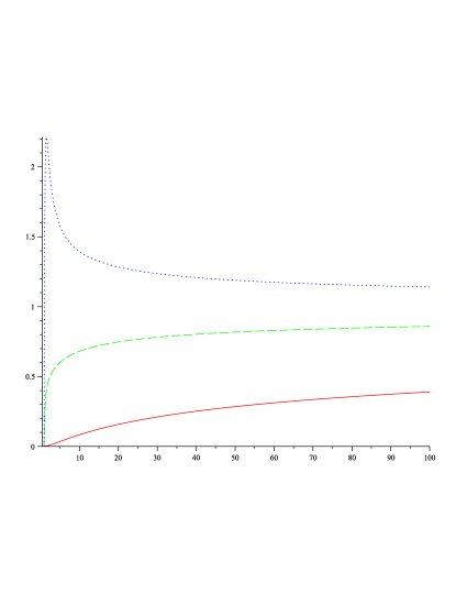
Figure 3: The plot of $f(r)$ versus $r$ for the different solutions in $4^{th}$-order quasitopological gravity for values of $k=1,0,-1$ (dot, dash, and solid respectively). Here, $r_{+}=0.9$, and $z=2$. The other parameters were $\hat{\mu}_{2}=0.04,\hat{\mu}_{3}=-0.001,\hat{\mu}_{4}=0.0003$.

In addition, we can explore the family of black hole solutions which arises as a result of the degeneracy in the Proca field boundary conditions Andrade2012 ; Keeler2012 . As mentioned in Brenna2011 , we have a set of black holes in which the metric functions differ for different “seed” values of the parameter $h_{0}$. We can explore how the $4^{th}$-order quasitopological parameter will alter the behaviour of this family of solutions.

Looking at a set of seed values in the range $h_{0}=\left[2.3,2.5\right]$, we see in figure 4 that the family of solutions still exists in quartic quasitopological gravity. The behaviour of the seed value also acts similarly; it allows some control over the initial spike of $f(r)$.

Overall an examination of the metric functions shows that the quartic quasitopological term, for the values studied, does not cause dramatically different solutions when compared to those obtained from cubic quasitopological gravity. This is not a disappointing conclusion; the ability to add a new parameter to the black hole without much additional cost could be important with respect to the gauge/gravity theory.

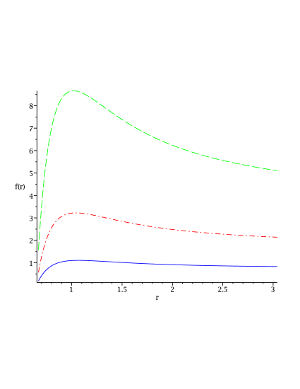
Figure 4: The plot of $f(r)$ versus $r$ for the different values of $h_{0}$: 2.5 (blue, solid), 2.3 (green, dashed), and 2.4 (red, dot-dash). Here, $r_{+}=0.65$, $k=1$, and $z=2$. The other parameters were $\hat{\mu}_{2}=0.2,\hat{\mu}_{3}=-0.001,\hat{\mu}_{4}=0.0005$ .

VII Thermodynamics

The entropy of the black hole solutions can be calculated through the use of the Iyer/Wald formula as Iyer

$$S=-2\pi\oint d^{n-1}x\sqrt{\tilde{g}}Y^{abcd}\hat{\epsilon}_{ab}\hat{\epsilon}_{cd},\hskip 14.22636pt\text{where}\hskip 5.69054ptY^{abcd}=\frac{\partial{\mathcal{L}}}{\partial{R_{abcd}}}$$ (42)

where $\mathcal{L}$ is the Lagrangian, $\tilde{g}$ is the determinant of the induced metric on the horizon and $\hat{\varepsilon}_{ab}$ is the binormal to the horizon.

Using the same prescription as Myers2010 , we obtain

$$\mathcal{S}=S/V_{n-1} =-2\pi r_{+}^{n-1}Y$$

$$=\frac{{r_{0}^{n-1}}}{4}\left(1+2\,k\hat{\mu}_{2}{\frac{\left(n-1\right){L}^{2}}{\left(n-3\right)r_{0}^{2}}}-3k^{2}\hat{\mu}_{3}{\frac{\left(n-1\right){\ L}^{4}}{\left(n-5\right)r_{0}^{4}}}+4{k}\hat{\mu}_{4}{\frac{\left(n-1\right){L}^{6}}{\left(n-7\right)r_{0}^{6}}}\right)$$ (43)

The temperature of the black holes, after Wick-rotation, is

$$T=\left(\frac{r^{z+1}\sqrt{f^{\prime}g^{\prime}}}{4\pi L^{z+1}}\right)_{r=r_{0}}.$$ (44)

We can produce plots to see the effect of the quartic quasitopological parameter on the thermodynamics of the black hole. In figure 5, we see that the positive quartic parameter continues to act in the same manner as before (i.e. as a “stronger” quasitopological addition) by pulling the black hole solution further from instability. Recall further that the slope of this graph indicates the sign of the specific heat, and that in the small-$r$ black hole (leftmost region) of the Einsteinian case, the negative slope means that the black hole is unstable.

Note that because the cosmological constant is specified by the quasitopological parameters, the different solutions do have different cosmological constants and therefore the plot does not converge to exactly the same black holes at large $r_{+}$ (on the right of the plot). However, if we were to find solutions with the same cosmological constant we would see that the large black holes would become thermodynamically identical. This is the expected result as the larger black holes will have reduced surface gravity and curvature so the higher order curvature terms will have reduced effect.

We also plot a comparison of black branes with different hypersurface curvature in figure 6. This shows the expected result that $k=-1$ is a stable solution while $k=1$ is stable for this particular set of parameters but appears to have the potential for instability.

Finally, a thermodynamics plot for $z=2$ was performed, which elucidates the $z=2$ behaviour of the quartic quasitopological term. Recall that in $z=2$ cubic quasitopological gravity Brenna2011 , instabilities in $k=1$ reappear depending on the strength of the cubic coupling term. We see the same behaviour with the quartic coupling term in figure 7. Though the slope of the curve is difficult to visually ascertain, an examination of the individual data points yields a transition from a negative to positive slope, as occurs for some values of $\hat{\mu}_{3}$ in $z=2$ cubic quasitopological gravity.

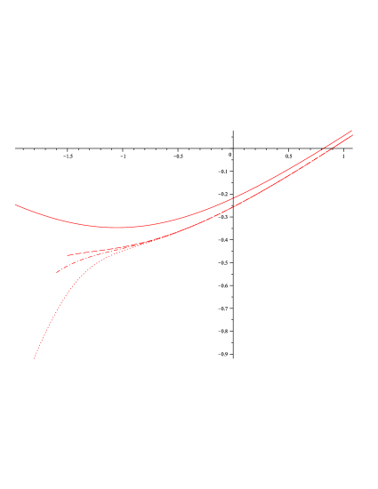
Figure 5: The plot of log($T$) versus log($S$) for higher-curvature black holes, where the solid line is Einsteinian, the dashed is Gauss-Bonnet, the dash-dot is $3^{rd}$ order quasitopological, and the dotted is $4^{th}$ order (quartic) quasitopological gravity. Here, $h_{0}=2.000$, $k=1$, $z=1$, and we are in 4+1 dimensions. The other parameters were $\hat{\mu}_{2}=0.04,\hat{\mu}_{3}=-0.001,\hat{\mu}_{4}=0.0004$.

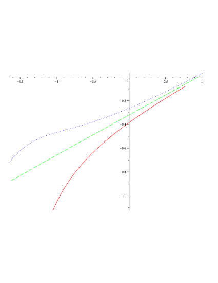
Figure 6: The plot of log($T$) versus log($S$) for higher-curvature black holes, where the solid line is $k=-1$, the dashed is $k=0$, the dotted is $k=1$ in $4^{th}$ order quasitopological gravity. Here, $h_{0}$ varies slightly for each solution, but is generally around $h_{0}\sim 0.560$, $z=1$, and we are in 4+1 dimensions. The other parameters were $\hat{\mu}_{2}=0.04,\hat{\mu}_{3}=-0.001,\hat{\mu}_{4}=0.0003$.

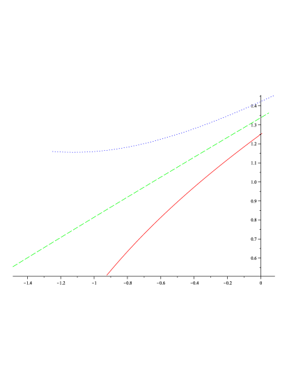
Figure 7: The plot of log($T$) versus log($S$) for higher-curvature black holes, where the solid line is $k=-1$, the dashed is $k=0$, the dotted is $k=1$ in $4^{th}$ order quasitopological gravity. Here, $h_{0}=0.724$, $z=2$, and we are in 4+1 dimensions. The other parameters were $\hat{\mu}_{2}=0.04,\hat{\mu}_{3}=-0.001,\hat{\mu}_{4}=0.0003$.

VIII Concluding Remarks

By using the Lifshitz metric in the spherically symmetric case, we considered the quartic quasitopological gravity and obtained the field equations. We then obtained the radially conserved quantity for quartic quasitopological Lifshitz theories. We investigated the existence of Lifshitz solutions both with and without massive background vector field and we found that a Lifshitz solution can be supported in vacuum under restrictions on the cosmological constant, Proca mass, and Proca charge. In the presence of the massive Abelian gauge field, after demonstrating that the quartic quasitopological gravity can support a Lifshitz solution, we numerically derived asymptotically Lifshitz black hole solutions, comparing them to previously published analytic solutions for consistency. We found that the $4^{th}-$order quasitopological term acts in a similar way as the $3^{rd}-$order term on metric functions of the black hole.

We can further summarize our findings for the thermodynamic effect of the quartic quasitopological parameter. In the context of cubic quasitopological results, the quartic term does not behave unexpectedly. Its ability to push solutions towards stability in $z=1$ and to generally affect stability in $z=2$ was seen.

Our conclusion is that the $4^{th}-$order theory adds yet another nontrivial parameter to the space of Lifshitz black hole solutions, which may be useful for obtaining multiple phase transitions, of use in a gauge/gravity duality. Now that a method of producing numerical solutions has been developed, this space of thermodynamic behaviour can be more fully explored. We leave this for future work.

References

(1) J. Maldacena, Adv. Theor. Math. Phys. 2, 231 (1998).
(2) J. Maldacena, Int. J. Theor. Phys. 38, 1113 (1999).
(3) J. L. Friedman, K. Schleich and D. M. Witt, Phys. Rev. Lett.
71, 1486 (1993)
(4) J. L. Friedman, K. Schleich and D. M. Witt, Phys. Rev. Lett.
75, 1872 (1995).
(5) T. Jacobson and S. Venkataramani, Class. Quant. Grav.
12, 1055 (1995).
(6) J. P. Lemos, Class. Quant. Grav. 12, 1081 (1995);
(7) J. P. Lemos, Phys. Lett. B 353, 46 (1995);
(8) J. P. S. Lemos and V. T. Zanchin, Phys. Rev. D 54, 3840 (1996).
(9) S. Aminneborg, I. Bengtsson, S. Holst and P. Peldan, Class. Quant. Grav.
13, 2707 (1996);
(10) R. B. Mann, Class. Quant. Grav. 14, L109 (1997);
(11) R. G. Cai and Y. Z. Zhang, Phys. Rev. D 54, 4891 (1996);
(12) M. H. Dehghani, Phys. Rev. D 65, 124002 (2002);
(13) M. H. Dehghani, Phys. Rev. D 66, 044006 (2002);
(14) M. H. Dehghani and A. Khodam-Mohammadi, Phys. Rev. D
67, 084006 (2003).
(15) W. G. Brenna and R. B. Mann, Phys. Rev. D 86, 064035 (2012).
(16) J. de Boera, M. Kulaxizia, and A. Parnachev, JHEP 06, 008 (2010).
(17) X. O. Camanho and J. D. Edelstein, JHEP 06, 099 (2010).
(18) M. H. Dehghani, A. Bazrafshan, R. B. Mann, M. R. Mehdizadeh,
M. Ghanaatian and M. H. Vahidinia, Phys. Rev. D 85, 104009 (2012).
(19) A. Bazrafshan, M. H. Dehghani, and M. Ghanaatian, Phys. Rev. D 86, 104043 (2012).
(20) M. Ghanaatian and A. Bazrafshan, Int. J. Mod. Phys. D
Vol. 22, No. 13, 1350076 (2013).
(21)
R. C. Myers and B. Robinson, JHEP 08, 067 (2010).
(22)
M. H. Dehghani and R. B. Mann, JHEP 07, 019 (2010).
(23)
W. G. Brenna, M. H. Dehghani, and R. B. Mann, Phys. Rev. D
84, 024012 (2011).
(24)
G. Dotti, J. Oliva, and R. Troncoso, Phys. Rev. D 76
064038 (2007).
(25) S. W. Hawking and D. N. Page, Commun. Math. Phys. 87, 577 (1983).
(26) E. Witten, Adv. Theor. Math. Phys. 2, 505 (1998).
(27) D. Birmingham, Class. Quant. Grav. 16, 1197
(1999).
(28) D. R. Brill, J. Louko and P. Peldan, Phys. Rev. D 56, 3600 (1997); A. Champlin, R. Emparan, C. V. Johnson and R. C.
Myers, ibid. 60, 064018 (1999).
(29) D. Lovelock, J. Math. Phys. 12, 498 (1971).
(30) M. H. Dehghani and R. B. Mann, Phys. Rev. D 73, 104003 (2006);
M. H. Dehghani, N. Alinejadi and S. H. Hendi, ibid.
77, 104025 (2008).
(31) R. G. Cai, Phys. Rev. D 65, 084014 (2002);
I. P. Neupane, ibid. 69, 084011 (2004).
(32) M. H. Dehghani and M. Shamirzaie, Phys. Rev. D 72, 124015 (2005).
(33) M. Banados, C. Teitelboim and J. Zanelli, Phys. Rev. D 49, 975 (1994).
(34) J. D. Bekenstein, Phys. Rev. D 7, 2333 (1973);
S. W. Hawking, Nature (London) 248, 30 (1974); G. W.
Gibbons and S. W. Hawking, Phys. Rev. D 15, 2738 (1977).
(35) M. Lu and M. B. Wise, Phys. Rev. D 47,
R3095 (1993); M. Visser, ibid. 48, 583 (1993).
(36) R. M. Wald, Phys. Rev. D 48, R3427, (1993).
(37) T. Jacobson and R. C. Myers, Phys. Rev. Lett. 70,
3684 (1993).
(38) R. A. Konoplya and A. Zhidenko, Phys. Rev. D 78, 104017 (2008);
D. Birmingham and S. Mokhtari, ibid. 76, 124039
(2007).
(39) S. S. Gubser and I. Mitra, JHEP 08, 018 (2001).
(40) V. Iyer and R. Wald, Phys. Rev. D 50, 846 (1994).
(41) T. Andrade and S. Ross, Class. Quant. Grav. 30, 065009 (2013).