Abstract

We show that the following algorithmic problem is decidable: given a $2$-dimensional simplicial complex, can it be embedded (topologically, or equivalently, piecewise linearly) in ${\mathbb{R}}^{3}$? By a known reduction, it suffices to decide the embeddability of a given triangulated 3-manifold $X$ into the 3-sphere $S^{3}$. The main step, which allows us to simplify $X$ and recurse, is in proving that if $X$ can be embedded in $S^{3}$, then there is also an embedding in which $X$ has a short meridian, i.e., an essential curve in the boundary of $X$ bounding a disk in $S^{3}\setminus X$ with length bounded by a computable function of the number of tetrahedra of $X$.

1 Introduction

The embeddability problem. Let EMBED_k→d be the following algorithmic problem: given a finite simplicial complex $K$ of dimension at most $k$, does there exist a (piecewise linear) embedding of $K$ into ${\mathbb{R}}^{d}$?

A systematic investigation of the computational complexity of this problem was initiated in [MTW11]; earlier it was known that EMBED_1→2 (graph planarity) is solvable in linear time, so is EMBED_2→2 [GR79], and for every $k\geq 3$ fixed, EMBED_k→2k can be decided in polynomial time (this is based on the work of Van Kampen, Wu, and Shapiro; see [MTW11]).

For dimension $d\geq 4$, there is now a reasonably good understanding of the computational complexity of EMBED_k→d: for all $k$ with $(2d-2)/3\leq k\leq d$ it is NP-hard (and even undecidable if $k\geq d-1\geq 4$) [MTW11], while for $k<(2d-2)/3$ it is polynomial-time solvable, assuming $d$ fixed, as was shown in a series of papers on computational homotopy theory [ČKM⁺13, ČKM⁺12, KMS13, ČKV13]. (However, the cases with $(2d-2)/3\leq k$ known to be NP-hard but not proved undecidable are still intriguing.)

Thus, the most significant gap up until now has been the cases $d=3$ and $k=2,3$, and in particular, after graph planarity (EMBED_1→2), the problem EMBED_2→3 can be regarded as the most intuitive and probably practically most relevant case.

Embeddability in ${\mathbb{R}}^{3}$. Here we close this gap, at least as far as decidability is concerned.

Theorem 1.1.

The problem EMBED_2→3 is algorithmically decidable. That is, there is an algorithm that, given a $2$-dimensional simplicial complex $K$, decides whether $K$ can be embedded (piecewise linearly, or equivalently, topologically) in ${\mathbb{R}}^{3}$.

Let us remark that one can naturally consider (at least) three different kinds of embeddings of a simplicial complex $K$ in ${\mathbb{R}}^{d}$, illustrated in the next picture for a $1$-dimensional complex (graph):

For linear embeddings, also referred to as geometric realizations, each simplex of $K$ should be mapped affinely to a (straight) geometric simplex in ${\mathbb{R}}^{d}$. This kind of embeddability is decidable in PSPACE regardless of the dimensions, and it is not what we consider here.

For piecewise linear, or PL, embeddings, one seeks a linear embedding of some (arbitrarily fine) subdivision of $K$. Finally, for a topological embedding, $K$ is embedded by an arbitrary injective continuous map.

While topological and PL embeddability need not coincide for some ranges of dimensions, for ambient dimension $d=3$, they do, and this is the notion of embeddability considered here.

An algorithm for EMBED_3→3 can be obtained from Theorem 1.1 by a simple reduction, given in Section 12.

Corollary 1.2.

The problem EMBED_3→3 is decidable as well.

Thickening to 3-manifolds. For a $2$-complex $K$, (PL) embeddability in ${\mathbb{R}}^{3}$ is easily seen to be equivalent to embeddability in $S^{3}$, and from now on, we work with $S^{3}$ as the target.

The first step in our proof of Theorem 1.1 is testing whether a given simplicial $2$-complex $K$ embeds in any 3-dimensional manifold at all.

Let us suppose that there is an embedding $f\colon K\to M$ for some $3$-manifold $M$ (without boundary), and take a sufficiently small closed neighborhood $X$ of the image $f(K)$ in $M$—the technical term here is a regular neighborhood. Then $X$ is a $3$-manifold with boundary, called a $3$-thickening of $K$.

There is an algorithm, due to Neuwirth [Neu68] (see also [Sko95] for an exposition) that, given $K$, tests whether it has any $3$-thickening, and if yes, produces a finite list of all possible $3$-thickenings, up to homeomorphism, as triangulated 3-manifolds with boundary (without the knowledge of $M$). Then $K$ embeds in $S^{3}$ iff one of its 3-thickenings does. Hence it suffices to prove the following.

Theorem 1.3.

There is an algorithm that, given a triangulated $3$-manifold $X$ with boundary, decides whether $X$ can be embedded in $S^{3}$.

Concerning the running time. Our proof does provide an explicit running time bound for the algorithm, but currently a rather high one, certainly primitive recursive but even larger than an iterated exponential tower. Thus, we prefer to keep the bounds unspecified, in the interest of simplicity of the presentation.

By refining our techniques, it might be possible to show the problem to lie in the class NP. Going beyond that may be quite challenging: indeed, as observed in [MTW11], EMBED_2→3 is at least as hard as the problem of recognizing $S^{3}$ (that is, given a simplicial complex, decide whether it is homeomorphic to $S^{3}$). The latter problem is in NP [Iva08, Sch04], but nothing more seems to be known about its computational complexity (e.g., polynomiality or NP-completeness).

Related work. There is a vast amount of literature on computational problems for $3$-manifolds and knots. Here we give just a sample; further background and references can be found in the sources cited below and in [AHT06]. A classical result is Haken’s algorithm deciding whether a given polygonal knot in ${\mathbb{R}}^{3}$ is trivial [Hak61]. More recently, this problem was shown to lie in NP [HLP99], and, assuming the Generalized Riemann Hypothesis, in coNP as well [Kup11]. The knot equivalence problem is also decidable [Hak61, Hem79, Mat97], but nothing seems to be known about its complexity status.

Closer in spirit to the problem investigated here are algorithms for deciding whether a given $3$-manifold is homeomorphic to $S^{3}$, already mentioned above [Rub95, Tho94, Iva08, Sch04].

An important special case of Theorem 1.3 is testing embeddability into $S^{3}$ for an $X$ whose boundary is a single torus; this amounts to recognizing knot complements and was solved in [JS03]. Some of the ideas in that work are used in our proof, but most of the argument is fairly different.

In a different direction, Tonkonog [Ton11] provided an algorithm for deciding whether a given 3-manifold $X$ with boundary embeds into some homology 3-sphere (which may depend on $X$). His methods are completely different from ours (except for using a 3-thickening to pass from 2-dimensional complexes to 3-manifolds), and it seems to be only loosely related to the problems investigated here.

Future directions. Besides the obvious questions of finding a more efficient algorithm, say one in NP, and/or proving hardness results, one may consider embeddability into other 3-manifolds $M$ besides $S^{3}$. We believe that this may be within reach of the methods used here, but definitely a number of issues would have to be settled.

The main technical contribution. Our algorithm relies on a large body of work in 3-dimensional topology.

When we talk about a surface in $X$, unless explicitly stated otherwise, we always mean a $2$-dimensional manifold $F$ with boundary properly embedded in $X$, that is, with $\partial F\subset\partial X$. Similarly, curves are considered properly embedded in a surface, so a connected curve can be a loop in the interior of the surface or an arc connecting two points of the boundary. Two properly embedded surfaces $F$ and $F^{\prime}$ are isotopic if they are embeddings of the same surface $F_{0}$ and there is a continuous family of proper embeddings $F_{0}\to X$ starting with $F$ and ending with $F^{\prime}$. An similar definition of isotopy applies to curves embedded in surfaces.

As in almost all algorithms working with 3-manifolds, we use Haken’s method of normal curves and surfaces, actually in a slightly extended form. Here we recall them very briefly; we refer to [Hem76, JT95] for background, and in Section 5 below we will discuss a variant.

A normal curve in a triangulated 2-dimensional surface $F$ intersects every triangle in finitely many disjoint pieces, which we can think of as straight segments, as in the left picture:

The main point is that such a curve is described, up to isotopy, purely combinatorially: namely, for every triangle $T$, there are just three types of segments of the curve inside, and it is enough to specify the number of segments for each type, for each $T$. In the picture, the numbers are $5,2,1$.

Similarly, a normal surface in a triangulated 3-manifold intersects each tetrahedron in finitely many of disjoint pieces, each of them a triangle or a quadrilateral, as in the right picture above. This time there are seven types of pieces, four triangular and three quadrilateral, per tetrahedron (although no two types of quadrilateral pieces may coexist in a single tetrahedron, since they would have to intersect, which is not allowed). So a normal surface $F$ in a 3-manifold with $t$ tetrahedra can be described by a vector of $7t$ nonnegative integers. This vector is called the normal vector of $F$.

A normal isotopy is an isotopy during which the intermediate curve or surface stays normal; in particular, it may not cross any vertex of the triangulation.

Going back to embeddings, we first simplify the situation using a result of Fox [Fox48], which allows us to assume that the complement of the supposed embedding of $X$ in $S^{3}$ is a union of handlebodies. (These handlebodies may be knotted or linked in $S^{3}$, though, as in the picture at the beginning of the next section.) This assumption is quite important and nontrivial; for example, we note that if $X$ is a solid torus, it can also be embedded in $S^{3}$ in a knotted way, so that the complement is not homeomorphic to a solid torus.

Thus, now we ask if there is a way of “filling” each component of $\partial X$ with a handlebody so that the resulting closed manifold is homeomorphic to $S^{3}$. Spherical boundary components are easy, since there is only one way, up to homeomorphism, of filling a spherical boundary component with a ball. However, already for a toroidal component there are infinitely many nonequivalent ways of filling it with a solid torus. Indeed, the filling can be done in such a way that a circle $\alpha$ on the toroidal component of $\partial X$, as in the left picture,

is identified with a curve $\beta$ on the boundary of the solid torus, shown in the right picture, where $\beta$ may wind around the solid torus as many times as desired. For boundary components of higher genus, there are also infinitely many ways of filling, and their description is still more complicated. For every specific way of filling the boundary components of $X$ with handlebodies we could test whether the resulting closed manifold is an $S^{3}$, but we cannot test all of the infinitely many possibilities. This is the main difficulty we have to overcome to get an algorithm.

Next, by more or less standard considerations, we can make sure that there is no “way of simplifying $X$ by cutting along a sphere or disk”—in technical terms, we may assume that $X$ is irreducible, that is, every $2$-sphere embedded in $X$ bounds a ball in $X$, and that $X$ has an incompressible boundary, i.e., any curve in $\partial X$ bounding a disk in $X$ also bounds a disk in $\partial X$.

For dealing with such an $X$, the following result is the key:

Theorem 1.4.

Let $X$ be an irreducible $3$-manifold, neither a ball nor an $S^{3}$, with incompressible boundary and with a $0$-efficient triangulation $\mathcal{T}$. If $X$ embeds in $S^{3}$, then there is also an embedding for which $X$ has a short meridian $\gamma$, i.e., an essential normal curve $\gamma\subset\partial X$ bounding a disk in $S^{3}\setminus X$ such that the length of $\gamma$, measured as the number of intersections of $\gamma$ with the edges of $\mathcal{T}$, is bounded by a computable function of the number of tetrahedra in $\mathcal{T}$.

In this theorem, $0$-efficient triangulation is a technical term introduced in [JR03], whose definition will be recalled later in Section 7. We are using $0$-efficient triangulations in order to exclude non-trivial normal disks and 2-spheres in $X$.

We should also mention that the triangulations commonly used in 3-dimensional topology, and also here, are not simplicial complexes in the usual sense—they are still made by gluing (finitely many) tetrahedra by their faces, but any set of gluings that produces a manifold is allowed, even those that identify faces of the same tetrahedron. As a result, a particular tetrahedron may not have four distinct faces, six distinct edges and four distinct vertices. In particular, 0-efficient triangulations of the manifolds we consider have a single vertex in each boundary component and none in the interior, all edges in the boundary form loops. This is the necessary result of modifying a triangulation by collapsing simplices, a triangular face to an edge or to a vertex, etc.; see [JR03, Sec. 2.1] for a thorough discussion. There is even a mind-boggling one-tetrahedron one-vertex triangulation of the solid torus obtained by gluing a pair of faces of a single tetrahedron, see [JS03].

Let us remark that $X$ as in the theorem need not have a short meridian for every possible embedding, even if we assume that the complement consists of handlebodies. For example, if $X$ is a thickened torus (a torus times an interval), we can embed it so that the curves bounding disks in $S^{3}\setminus X$ are arbitrarily long w.r.t. a given triangulation of $X$. We must sometimes change the embedding to get short meridians.

It is also worth mentioning that this problem does not occur if $\partial X$ is a single torus, i.e., the knot complement case. Here a celebrated theorem of Gordon and Luecke [GL89] makes sure that there is only one embedding, up to a self-homeomorphism of $S^{3}$, and the meridian is unique up to isotopy. This is why the single-torus boundary case solved in [JS03] is significantly easier than the general case.

2 An outline of the arguments

Our algorithm for Theorem 1.3, deciding the embeddability of a given $3$-manifold $X$ in $S^{3}$, for the case of $X$ irreducible and with incompressible boundary, consists in testing every possible normal curve $\gamma\subset\partial X$ of length bounded as in Theorem 1.4. For each such candidate $\gamma$, we construct a new manifold $X^{\prime}=X^{\prime}(\gamma)$ by adding a $2$-handle to $X$ along $\gamma$, which means that we glue a disk bounded by $\gamma$ to the outside of $X$ and thicken it slightly, as illustrated in the following picture:

Here $X$ is the complement of the union of two (linked) handlebodies, a knotted solid 3-torus and a solid torus, and for $X^{\prime}$, the solid 3-torus in the complement has been changed to a solid double torus.

Then we test the embeddability of each $X^{\prime}(\gamma)$ recursively, and $X$ is embeddable iff at least one of the $X^{\prime}(\gamma)$ is. It is not hard to show that the algorithm terminates, using the vector of genera of the boundary components of $X$; see Section 3.

The proof of Theorem 1.4 occupies most of the paper and has many technical steps. In this section we give an outline.

We assume $X$ to be embedded in $S^{3}$, the complement being a union of handlebodies, and we apply a result of Li [Li10] stating that there is a planar surface (i.e., a disk with holes) $P\subset X$ that is “stuck” in its position in a suitable sense (namely, $P$ is either essential, or strongly irreducible and boundary strongly irreducible) and is meridional or almost meridional.

Here an essential curve $\gamma\subset\partial X$ is a meridian in a given embedding of $X$ in $S^{3}$ if it bounds a disk in $S^{3}\setminus X$. The surface $P$ is meridional if each component of $\partial P$ is a meridian, and it is almost meridional if all components of $\partial P$ but one are meridians. (Actually, Li has yet another case in his statement, but as we will check, that case can be reduced to the ones given above; see Lemma 4.4.) The next picture illustrates a meridional $P$ in the case where $X$ is embedded in $S^{3}$ as the complement of a solid torus neighborhood of the figure ‘8’ knot:

Next, by choosing $P$ as above with suitable minimality properties, one can make sure that $P$ is normal or almost normal for the given triangulation. For the case of $P$ essential, this is an old result going back to Haken and Schubert (and for our notion of complexity of $P$, a proof is given in Section 7), while for $P$ strongly irreducible and boundary strongly irreducible this follows from [BDTS12]; also see [Sto00] for the case of a strongly irreducible surface in a closed manifold. It remains to show that, in this setting, at least one of the meridians in $\partial P$ must be short.

Here we apply an average length estimate, which is an idea of Jaco and Rubinstein appearing in [JS03, JRS09].

Let $\gamma_{1},\ldots,\gamma_{b}$ be the components of $\partial P$, and let $\ell(\partial P)=\sum_{i=1}^{b}\ell(\gamma_{i})$ be the boundary length of $P$. We know that all the $\gamma_{i}$ but at most one are meridians. The length of the shortest meridian is bounded by the average $\ell(P)/(b-1)$, and we want to bound this average by a (computable) function of $t$, the number of tetrahedra in the triangulation $\mathcal{T}$ of $X$.

Now by the theory of normal surfaces, the (almost) normal surface $P$ can be written as a normal sum of fundamental surfaces in $X$,

$$P=\sum_{i}k_{i}F_{i},$$ (1)

where the $k_{i}$ are positive integers and the $F_{i}$ are surfaces from a finite collection; their number, as well as ${\ell_{\rm max}}:=\max_{i}\ell(\partial F_{i})$ can be bounded by a (computable) function of $t$ alone, and does not depend on $P$.

Since the boundary length is additive w.r.t. normal sum, we have $\ell(\partial P)=\sum_{i}k_{i}\ell(\partial F_{i})\leq{\ell_{\rm max}}K$, where $K:=\sum_{i}k_{i}$ is the number of fundamental summands in the expression for $P$, and so it suffices to show that $K\leq Cb$, with some computable function $C=C(t)$.

The basic version of the average-length estimate uses the Euler characteristic $\chi$ as an accounting device. Since $\chi$ is additive as well, $\chi(P)=\sum_{i}k_{i}\chi(F_{i})$. Since $P$ is a planar surface with $b$ boundary components, we have $\chi(P)=2-b$.

Now an ideal situation for the average-length estimate (which we cannot guarantee in our setting) is when $\chi(F_{i})\leq-1$ for every $i$; in other words, none of the summands is a disk, 2-sphere, annulus, Möbius band, or torus (or projective plane or Klein bottle, but these cannot occur in $X$ embedded in $S^{3}$). Then we get $b-2=-\chi(P)=\sum_{i}k_{i}(-\chi(F_{i}))\geq K$, and we are done (even with $C=1$).

In our actual setting, the summands with $\chi>0$, i.e., spheres and disks, are excluded by the $0$-efficient triangulation of $X$. We also need not worry about torus summands, since they have empty boundary and thus do not contribute to $\ell(\partial P)$. The real problem are annuli (and Möbius bands, but since twice a Möbius band, in the sense of normal sum, is an annulus, Möbius bands can be handled easily once we deal with annuli).

There are two kinds of annuli, which need very different treatment: the essential ones, and the boundary parallel ones. Here an annulus $A\subset X$ is boundary parallel if it can be isotoped to an annulus $A^{\prime}\subset\partial X$ with $\partial A^{\prime}=\partial A$ while keeping the annulus boundary fixed. Boundary parallel annuli do not occur for $P$ essential, but they might occur for the case of $P$ strongly irreducible and boundary strongly irreducible.

To deal with the annulus summands, we first construct what we call an annulus curve $\alpha\subset\partial X$. This is the boundary of a maximal collection $\mathcal{A}$ of essential annuli, maximal in the sense that each of the two boundary curves of every other essential annulus, after a suitable normalization, either intersects $\alpha$ or is normally isotopic to a component of $\alpha$. We bound the length of $\alpha$ by a computable function of $t$, and $|\alpha\cap P|$, the number intersections of $\alpha$ with $P$, by $C^{\prime}b$, for some computable $C^{\prime}=C^{\prime}(t)$, again assuming $P$ minimal in a suitable sense. For obtaining this bound we may need to change the embedding of $X$, and we also use results about “untangling” a system of curves on a surface by a boundary-fixing self-homeomorphism from [MSTW13].

Similarly, we construct a collection $\Gamma$ of curves that helps to deal with boundary parallel annuli: those that have minimal boundary in a suitable sense either intersect $\alpha$, or their boundaries are normally isotopic to components of $\alpha$ or curves from $\Gamma$.

Having constructed such an $\alpha$ and $\Gamma$, we work with normal curves and surfaces in a “marked” sense, which also takes into account the position of the curves and surfaces w.r.t. $\alpha$ and $\Gamma$. This, in particular, makes the number of intersections with $\alpha$ additive w.r.t. the marked normal sum, which in turn allows us to bound the number of annulus summands in (1), both boundary parallel and essential, that intersect $\alpha$ by $C^{\prime}b$.

Then we might have boundary-parallel annulus summands that avoid $\alpha$, but we show that those do not occur at all, since they would contradict the minimality of $P$.

Finally, there remain essential annuli that have a boundary component parallel to a component of $\alpha$. Here we show that if such an annulus had the coefficient $k_{i}$ in (1) at least $|\alpha\cap\partial P|\leq C^{\prime}b$, then there is a self-homeomorphism of $X$, namely, a Dehn twist in the annulus, that makes $P$ simpler, contradicting its supposed minimality. (Here we may again modify the assumed embedding of $X$ in $S^{3}$ in order to get a short meridian—and, as we have remarked, some such modification is necessary in the proof, since some embeddings may not have short meridians.) Hence for these essential annuli, too, the coefficients are bounded by a linear function of $b$. This concludes the proof.

3 The algorithm

If $X$ embeds in $S^{3}$, then it is orientable, and orientability can easily be tested algorithmically (e.g., by a search in the dual graph of the triangulation, or by computing the relative homology group $H_{3}(X,\partial X)$). So from now on, we assume $X$ orientable. In this situation, the boundary of $X$ is a compact orientable 2-manifold, and thus each component is a 2-sphere with handles.

We describe a recursive procedure EMB(X) that accepts a triangulated orientable 3-manifold with boundary and returns TRUE or FALSE depending on the embeddability of $X$ in $S^{3}$. (With some more effort, for the TRUE case, we could also recover a particular embedding, but we prefer simplicity of presentation.) The procedure works as follows.

1. (Each component separately) Let $X_{1},\ldots,X_{k}$ be the connected components of $X$. If $k>1$, test if there is an $S^{3}$ among the $X_{i}$ (several algorithms are available for that [Rub95, Tho94, Iva08, Sch04]), and if yes, return FALSE. Otherwise, still for $k>1$, return the conjunction ${\tt EMB}(X_{1})\wedge\cdots\wedge{\tt EMB}(X_{k})$.

2. (Fill spherical holes) Now we have $X$ connected. If it is an $S^{3}$, return TRUE. If there are components of $\partial X$ that are $S^{2}$’s, form $X^{\prime}$ by attaching a 3-ball to each spherical component of $\partial X$, and return ${\tt EMB}(X^{\prime})$.

3. (Connected sum) Form a decomposition $X=X_{1}\#\cdots\#X_{k}$ of $X$ into a connected sum of prime manifolds that are not $3$-spheres. If $k>1$, i.e., $X$ is not prime, return ${\tt EMB}(X_{1})\wedge\cdots\wedge{\tt EMB}(X_{k})$. If $X$ is prime but not irreducible, i.e., contains an $S^{2}$ that does not bound a ball, then return FALSE.

4. (Boundary compression) Test if there is a compressing disc $D$ for $\partial X$ (i.e., $\partial D\subset\partial X$ does not bound a disk in $\partial X$). If yes, cut $X$ along $D$, obtaining a new manifold $X^{\prime}$. Three cases may occur:

   1. If $X^{\prime}$ has two components, $X^{\prime}_{1}$ and $X^{\prime}_{2}$, return ${\tt EMB}(X^{\prime}_{1})\wedge{\tt EMB}(X^{\prime}_{2})$. This case may occur, for example, for $X$ a handlebody with two handles (a “thickened 8”) when $D$ separates the two handles.

   2. If $X^{\prime}$ is connected and the two “scars” after cutting along $D$ lie in the same component of $\partial X^{\prime}$, return EMB$(X^{\prime})$. This case may occur, e.g., for $X$ a solid torus.

   3. If neither of the previous two cases occur, then $X^{\prime}$ is connected but the scars lie in different components of $\partial X^{\prime}$. Return FALSE. To get an example of $X$ fitting this case, we can start with a thickened torus (i.e., torus times $[-1,1]$) and connect the two boundary components by a $1$-handle—which cannot be done in ${\mathbb{R}}^{3}$, but it does give a 3-manifold (with double torus boundary).

5. (Short meridian) Now $X$ is irreducible and with incompressible boundary. Using [JR03, Thm. 5.20], retriangulate $X$ with a $0$-efficient triangulation. Then proceed as described at the beginning of Section 2: let $\gamma_{1},\ldots,\gamma_{n}$ be a list of all closed essential normal curves in $\partial X$ up to the length bound as in Theorem 1.4, for each $i$ form $X^{\prime}(\gamma_{i})$ by attaching a $2$-handle along $\gamma_{i}$, and return the disjunction ${\tt EMB}(X^{\prime}(\gamma_{1}))\vee\cdots\vee{\tt EMB}(X^{\prime}(\gamma_{n}))$.

Lemma 3.1.

The above procedure always terminates and returns a correct answer, assuming the validity of Theorem 1.4.

Proof.

First we show that the algorithm always terminates. Let $C_{1},\ldots,C_{k}$ be the components of $\partial X$ numbered so that $g(C_{1})\geq\cdots\geq g(C_{k})$, where $g(.)$ stands for the genus, and let $\vec{g}_{\geq}(X)$ be the vector $(g(C_{1}),\ldots,g(C_{k}))$. We consider these vectors ordered lexicographically (if two vectors have a different length, we pad the shorter one with zeros on the right).

Let us think of the computation of the algorithm as a tree, with nodes corresponding to recursive calls. The branching degree is finite, so it suffices to check that every branch is finite.

It is easy to see that $\vec{g}_{\geq}(X)$ cannot increase by passing to a connected component or to a prime summand, and that it decreases strictly by a boundary compression and also by the short meridian step. Indeed, we observe that in the boundary compression step or the short meridian step, exactly one of the boundary components $C_{i}$ is affected, and it is either split into two components $C^{\prime}$ and $C^{\prime\prime}$ of nonzero genus and with $g(C_{i})=g(C^{\prime})+g(C^{\prime\prime})$, or it remains in one piece but the genus decreases by one. Since after steps 1–3 we have a connected irreducible manifold without spherical boundary components, for which the next step either finishes the computation or reduces $\vec{g}_{\geq}(X)$ strictly, every branch is finite as needed.

It remains to show that the returned answer is correct. For Step 2, we need that there is a unique way of filling a spherical hole; this is well known and can be inferred, for example, from the fact that there is only one orientation-preserving self-homeomorphism of $S^{2}$ up to isotopy [FM11, Sec. 2.2].

For Step 3, it is easily checked that a connected sum embeds iff the summands do. Moreover, every $S^{2}$ embedded in $S^{3}$ separates it, and hence if $X$ contains a non-separating $S^{2}$, then it is not embeddable.

For Step 4, it is clear that if $X$ is embeddable, then so is $X^{\prime}$.

If, in case (4a), $X^{\prime}_{1}$ and $X^{\prime}_{2}$ are both embedded, then it is easy to construct an embedding of $X$: Denote $D$’s scars by $D_{1}$ and $D_{2}$. Then a regular neighborhood of $D_{i}$ is a ball $B_{i}$ with boundary $S_{i}=\partial B_{i}$, and that meets both $X^{\prime}_{i}$ and $S^{3}\setminus X^{\prime}_{i}$ in balls. Think of each $X^{\prime}_{i}$ as embedded in its own copy of $S^{3}$, and take a connected sum of these two $S^{3}$’s so that $S^{3}=S^{3}\#S^{3}\supset X^{\prime}_{1}\#_{D_{1}=D_{2}}X^{\prime}_{2}=X$. Similarly, if $X^{\prime}$ is embedded in case (4b), then we can connect the scars by a thin handle in $S^{3}\setminus X^{\prime}$ and obtain an embedding of $X$.

In case (4c), let $C_{1}\neq C_{2}$ be the components of $\partial X^{\prime}$ containing the scars. Since the disk $D$ does not separate $X$, we can choose a loop $\delta\subset$X meeting $D$ in a single point, and such that $\delta$ also meets $C_{1}$ in a single point. But then, if $X$ were embedded in $S^{3}$, $C_{1}$ would yield a nonseparating surface in $S^{3}$—a contradiction.

Finally, if one of the $X^{\prime}(\gamma_{i})$ is embeddable in Step 5, then so is $X$ (since in $X^{\prime}$ we have $2$-handle that was added to $X$, and we can just assign it to the complement of $X$), and if $X$ is embeddable, then at least one of the $X^{\prime}(\gamma_{i})$ is by Theorem 1.4. ∎

4 Intersections of curves and surfaces

In this section we collect terminology, definitions and basic results concerning properly embedded curves in surfaces and properly embedded surfaces in 3-manifolds. In particular, for latter sections we need that any pair of properly embedded surfaces, each either essential, or, strongly irreducible and boundary strongly irreducible, can be isotoped to intersect essentially. There are few new results in this section. The reader is referred to Hempel [Hem76] and Jaco [Jac80] for more background.

We assume throughout that all curves and surfaces have been isotoped to have transverse intersection.

4.1 Curves

A curve is a properly embedded $1$-dimensional manifold in a surface $F$, each component either a loop, which is closed, or an arc, which has two endpoints in $\partial F$.

A loop is trivial if it bounds a disk in $F$ and an arc is trivial if it co-bounds a disk in $F$ with some arc in $\partial F$. A curve is essential if no component is trivial.

Pairs of curves are assumed to intersect transversally. If $\alpha$ and $\beta$ are a pair of curves, then their geometric intersection number $i(\alpha,\beta)=\min(|\alpha^{\prime}\cap\beta^{\prime}|)$ taken over all pairs of curves $(\alpha^{\prime},\beta^{\prime})$ where $\alpha^{\prime}$ and $\beta^{\prime}$ are isotopic to $\alpha$ and $\beta$ within $F$, respectively. (The isotopies are also allowed to move endpoints of arcs within the boundary.)

We say that $\alpha$ and $\beta$ bound a bigon if there is a disk bounded by a pair of sub-arcs, one from each curve; see Figure 3 in Section 6 below. We say that they bound a half-bigon if there is a disk bounded by a pair of sub-arcs, one from each curve, along with an arc in $\partial F$. If $\alpha$ and $\beta$ bound a bigon or half-bigon, then they can be isotoped to reduce their intersection.

We need this converse, a mild generalization of Farb and Margalit’s bigon criterion:

Lemma 4.1 (Bigon criterion [FM11]).

A pair of curves $\alpha$ and $\beta$ realize their geometric intersection number if and only if they do not bound a bigon or half-bigon.

Proof.

Farb and Margalit show that any pair of connected loops that intersect non-minimally form a bigon. They also note that this extends to disconnected curves consisting of loops.

If either curve has an arc component, then the doubled curves are properly embedded closed curves in the double of the surface. If they intersect non-minimally in the original, they intersect non-minimally in the double and hence bound a bigon there. Thus, they bound a half-bigon in the original. ∎

4.2 Essential surfaces

We will assume that our surfaces are properly embedded in a 3-manifold $X$ that is irreducible, i.e., every sphere embedded in $X$ bounds a ball in $X$, and boundary incompressible, i.e., any curve in $\partial X$ bounding a disk in $X$ also bounds a disk in $\partial X$ (is trivial).

Let $F$ be a surface properly embedded in $X$. A compressing disk for a $F$ is an embedded disk $D\subset X$ whose interior is disjoint from $F$ and whose boundary is an essential loop in $F$. A boundary compressing disk is an embedded disk $D\subset X$ whose boundary, $\partial D=f\cup x$, is the union of $f=\partial D\cap F=D\cap F$, an essential arc properly embedded in $F$, and $x=\partial D\cap\partial X=D\cap F$, an arc properly embedded in $\partial X$. Here is an illustration:

A surface $F$ is compressible if it has a compressing disk, boundary compressible if it has a boundary compressing disk, and incompressible and boundary incompressible if not, respectively. A surface is essential if it is incompressible, boundary incompressible, and not a sphere bounding a ball, or a disk co-bounding a ball with a disk in $\partial X$.

We establish some basic facts about surfaces in $X$.

Proposition 4.2.

The following statements hold for properly embedded surfaces in $X$, an irreducible, orientable $3$-manifold with non-empty incompressible boundary:

1. Every disk co-bounds a ball with a disk in $\partial X$.

2. Every connected surface with an inessential boundary curve is either compressible or a disk.

3. The boundary curve of every compressible annulus is trivial in $\partial X$boundary.

4. Every boundary compressible annulus is boundary parallel (parallel to an annulus in $\partial X$).

5. No surface is a projective plane.

6. Every Möbius band is essential.

Proof.

Because $X$ has incompressible boundary, the boundary of a properly embedded disk bounds a disk in $\partial X$. The union of these disks is a sphere that, because $X$ is irreducible, bounds a ball, yielding (i).

For (ii), suppose that some boundary curve of connected $F$ bounds a disk in $\partial X$. Then, among disks in $\partial X$ bounded by boundary curves of $F$, an innermost such disk can be pushed slightly into the interior of $X$ while keeping its boundary in $F$. The boundary curve is either trivial in $F$, in which case $F$ is a disk, or essential in $F$, in which case $F$ is compressible.

Concerning (iii), let $D$ be a compressing disk for an annulus $A$. Then $\partial D$ separates $A$ into two annuli $A^{\prime}$ and $A^{\prime\prime}$. So $D\cup A^{\prime}$ and $D\cup A^{\prime\prime}$ are properly embedded disks, each with one boundary curve of $A$. Because $\partial X$ is incompressible, the boundary curves are both trivial in $\partial X$.

As for (iv), let $B$ be a boundary compressing disk for an annulus $A$. Then $\partial N(A\cup B)$, the boundary of a regular neighborhood of their union, has two components, an annulus isotopic to $A$ and a disk. By (i), the disk co-bounds a ball with a disk in $\partial X$. But then the union of $N(A\cup B)$ with the ball is a solid torus, across which $A$ is parallel to an annulus in $\partial X$.

Concerning (v), if $P$ is a projective plane, then $\partial N(P)$, the boundary of its regular neighborhood, is a sphere which separates $P$ from $\partial X$. Then $X$ is reducible, for the sphere cannot bound a ball—no ball has interior boundary or contains an embedded projective plane.

Finally, in (vi), let $M$ be a a Möbius band. Suppose first that $M$ is compressible and let $D$ be a compressing disk for $M$. Then $\partial D$ cannot meet $M$ in a core curve of $M$ for this would imply that the core curve is orientation reversing in $X$. So $\partial D$ is a 2-sided curve in $M$ and separates it into an annulus and a narrower Möbius band $M^{\prime}$. Then the union $M^{\prime}\cup D$ is an embedded projective plane contradicting (v).

Suppose a Möbius band $M$ is boundary compressible. Then $\partial N(M)$ is a boundary compressible annulus $A$. By (iv), $A$ is boundary parallel, and co-bounds an solid torus with an annulus in the boundary. But the parallel region cannot contain the Möbius band $M$, and hence $X$ is the union of two solid tori, $N(M)$ and the solid torus parallel region. ∎

We say that a a pair of surfaces, $F$ and $G$, intersect essentially if each component of the curve $F\cap G$ is essential in both $F$ and $G$ (they are allowed to be disjoint). It is well known that essential surfaces can be arranged to intersect essentially:

Lemma 4.3.

Let $F$ and $G$ be properly embedded essential surfaces in an irreducible manifold with incompressible boundary. Then $G$ can be isotoped so that they intersect essentially.

Proof.

Assume that we have isotoped $G$ to minimize the number of curve components in $F\cap G$. We will show by contradiction that $F$ and $G$ intersect essentially.

We first note that if there is an intersection curve that is inessential in $F$, then there is an intersection curve that is inessential in $G$ and vice-versa: If an intersection curve bounds a disk in $F$, choose one whose disk is innermost. Since $G$ is incompressible, this disk is not a compressing disk for $G$ and it follows that its boundary, an intersection loop, is inessential in $G$. The same observation applies to inessential intersection arcs.

Then, assuming that some intersection loop is trivial, we can pass to one that is innermost on $F$, i.e., choose $\alpha$ to be an intersection loop that bounds a disk $D\subset F$ whose interior is disjoint from $G$. Since $G$ is not compressible, $\alpha$ also bounds a disk $D^{\prime}\subset G$. The union $D\cup D^{\prime}$ is a sphere that, because $X$ is irreducible, bounds a ball. And there is an isotopy of $G$ that is restricted to a neighborhood of $D^{\prime}$, and that pushes $D^{\prime}$ across the ball and past $D$. This isotopy of $G$ eliminates $\alpha$ and any other intersection curves in the interior of $F\cap D^{\prime}$, and it does not introduce any new intersection curves since $\alpha$ was innermost.

Now assume some intersection arc is trivial in one of the surfaces, and as noted, we can let $\alpha$ denote such an arc that is outermost in $F$. That is, $\alpha$ cuts off a disk $D\subset F$ whose interior is disjoint from $G$ and whose boundary meets $\partial X$ in an arc. And $\alpha=D\cap G$ cuts off a, not necessarily outermost, disk $D^{\prime}\subset G$ that also meets $\partial X$ in an arc.

The union $D\cup D^{\prime}$ is a disk with its boundary in $\partial X$ that, because $\partial X$ is incompressible, bounds a disk $D^{\prime\prime}\subset\partial X$. Since $X$ is irreducible, $D\cup D^{\prime}\cup D^{\prime\prime}$ is a sphere bounding a ball. Moreover, there is an isotopy of $G$ that pushes a neighborhood of $D^{\prime}$ past $D$ and outside the ball. ∎

4.3 Almost meridional surfaces

Suppose that $X$ is an irreducible manifold with incompressible boundary that is embedded in $S^{3}$. We recall that an essential curve $\mu\subset\partial X$ is a meridian if it bounds a disk in $S^{3}\setminus X$. A properly embedded surface is meridional if each of its boundary curves is a meridian, and almost meridional if all but exactly one of its boundary curves is a meridian.

Let $D$ be a boundary compressing disk for an orientable surface $P$. Then $\partial N(P\cup D)$ is a surface with at least two components. One component is isotopic to $P$; let $P^{\prime}$ be the union of the other components. Then $P^{\prime}$ is said to be the result of boundary compressing $P$ along $D$.

Lemma 4.4.

Suppose that a manifold $X$ is embedded in $S^{3}$. If $P$ is a connected almost meridional planar surface properly embedded in $X$, then any surface $P^{\prime}$ obtained by boundary compressing $P$ contains an almost meridional component.

Proof.

Let $P^{\prime}$ be obtained from $P$ by boundary compressing along the disk $D$. What happens to $\partial P$? The disk $D$ meets at most two boundary components of $\partial P$. Any component not met by $D$ has two parallel copies in $\partial N(P\cup D)$, one for $P$ and one for $P^{\prime}$, so those are unchanged. Let $\beta$ be the one or two loops meet by the arc $x=D\cap\partial X$. Since $D$ lies on one side of the the 2-sided planar surface $P$, when $\beta$ is a single loop, $x$ approaches it twice from the same side. It follows that $\partial N(x\cup\beta)$ is a pair of pants, i.e., an $S^{2}$ with three holes bounded by loops. One of these loops belongs to $P$ and two to $P^{\prime}$, or vice-versa.

If any two of these three loops are meridians, then so is the third, since it bounds a disk, namely the union of the pants and the two disks pushed slightly into $S^{3}\setminus\mathrm{interior}(X)$.

We apply this “two meridians implies three meridians” principle to show that $P^{\prime}$ has an almost meridional component, regardless of how the boundary compressing disk meets the boundary components of $P$.

If the boundary compressing disk meets the non-meridional component twice, then the compression eliminates the non-meridional curve, and creates two new curves, each belonging to a separate component of $P^{\prime}$. At least one of the new curves is not meridional, and hence its component is almost meridional.

If the boundary compressing disk meets a meridian and the non-meridian, then the compression does not separate $P$, and trades these curves for a new non-meridional curve. Thus $P^{\prime}$ is almost meridional.

If the boundary compressing disk meets two distinct meridians, then they are eliminated and a new one is created. The connected surface $P^{\prime}$ is almost meridional.

If the boundary compressing disk meets a single meridian twice, then $P^{\prime}$ has two components, each with one of the two new curves, either both meridional or both non-meridional. If both are meridional, then the component with the original non-meridian on its boundary is almost meridional. If both are non-meridional, then the component without the original non-meridian is almost meridional. One of the two components of $P^{\prime}$ is almost meridional. ∎

Lemma 4.5.

Suppose that $X$, an irreducible manifold with incompressible boundary, is embedded in $S^{3}$. If $X$ contains an incompressible, almost meridional planar surface, then $X$ contains an essential almost meridional planar surface.

Proof.

An incompressible almost meridional surface can be sequentially boundary compressed until it is incompressible and boundary incompressible. By the prior lemma, each surface in the sequence, hence the final one, has an almost meridional component. This final component is not a disk because $X$ is boundary incompressible. Hence it is an essential almost meridional planar surface. ∎

4.4 Strongly irreducible surfaces

A two-sided surface properly embedded in $X$ is bi-compressible if it has a compressing pair $(D_{+},D_{-})$, a pair of disks, each a compressing or boundary compressing disk, one for each side of the surface. The pair is simultaneous if $\partial D_{+}\cap\partial D_{-}=\emptyset$.

A surface is weakly reducible if it is simultaneously bi-compressible using compressing disks only. A strongly irreducible surface is one that is bi-compressible using compressing disks but not simultaneously so. A surface is boundary weakly reducible if it is simultaneously bi-compressible using any combination of compressing disks and boundary compressing disks. A surface is boundary strongly irreducible if it is bi-compressible, using any combination of compressing or boundary compressing disks, but not simultaneously so.

Some of our results assume that a surface is both strongly irreducible and boundary strongly irreducible. It may seem that the strongly irreducible hypothesis is vacuous. But this is not the case—it guarantees that the surface has at least one (non-boundary) compressing disk for each side.

Lemma 4.6 ([BDTS12], Lemma 3.8).

In an irreducible manifold with incompressible boundary, the boundary of a strongly irreducible surface is essential in the boundary of the manifold.

We state here a special case of Lemma 4.2 of [Bac13]. This

Lemma 4.7 (Lemma 4.2 of [Bac13]).

Let $F$ be an essential surface and $G$ a surface that is strongly irreducible and boundary strongly irreducible. Then $G$ may be isotoped so that $F$ and $G$ intersect essentially.

Let us remark that Bachman does not give a proof but claims it to be a direct generalization of [Bac09, Corol. 3.8]. He has also provided us with an unpublished manuscript with a proof.

5 Theory of normal curves and surfaces in a marked triangulation

In this section we introduce a mild generalization of the theory of normal curves and surfaces.

Definition 5.1.

A marked triangulation is a pair $(\mathcal{T},M)$ consisting of a triangulation $\mathcal{T}$ of a $2$- or $3$-manifold along with a marking $M\subset\mathcal{T}^{1}$, a finite set of points along the edges of $\mathcal{T}$.

If $M=\emptyset$, then $(\mathcal{T},M)$ is a triangulation in the usual sense and we will usually omit $M$ and refer directly to $\mathcal{T}$. Similarly, when $M=\emptyset$, we will describe objects as being normal rather than $M$-normal, and note that our definitions restrict to the standard ones.

An arc in a triangle is $M$-normal if its endpoints lie in distinct edges of the face and it misses $M$. A properly embedded curve $\alpha$ in the boundary surface is $M$-normal if it is the union of $M$-normal arcs. The length of $\alpha$, $\ell(\alpha)=|\alpha\cap\mathcal{T}^{1}|$, is its number of intersections with the 1-skeleton.

There are several types of elementary surfaces contained in a tetrahedron $\Delta$. An $M$-normal disk is a disk in $\Delta$ whose boundary is an $M$-normal curve of length 3 or 4 in $\partial\Delta$. We also consider two types of $M$-exceptional pieces: An octagon is a disk in $\Delta$ whose boundary is an $M$-normal curve of length 8 in $\partial\Delta$. A tube is an unknotted annulus in $\Delta$ whose boundary consists of two $M$-normal curves whose total length is at most 8.

An $M$-normal surface is a properly embedded surface that is the union of $M$-normal disks. An almost $M$-normal surface is a properly embedded surface that is the union of a single $M$-exceptional piece and a collection of $M$-normal disks.

The weight of an (almost) $M$-normal surface $A$ is $\operatorname{wt}(A)=|A\cap\mathcal{T}^{1}|$, the number of intersections with the 1-skeleton. Its length is the length of its boundary: $\ell(A):=\ell(\partial A)$.

An $M$-normal isotopy is a normal isotopy that does not pass through any point in $M$. An $M$-type is the equivalence class of an $M$-normal arc in a face, or, an $M$-normal disc or $M$-exceptional piece in a tetrahedron. Two types are $M$-compatible if they have disjoint representatives. A pair of curves or surfaces are $M$-compatible if each pair of types they possess are $M$-compatible. That is, a pair of curves is $M$ compatible if, for each face of the triangulation, their arcs in that face are pairwise disjoint after an $M$-normal isotopy. An analogous statement holds for surfaces.

We note that $M$-compatibility is a local condition; in general it may not be possibly to make $M$-compatible curves or surfaces globally disjoint by an $M$-normal isotopy.

The $M$-normal vector or $M$-normal coordinates of an $M$-normal curve, surface, or almost $M$-normal surface $A$ is a uniquely determined vector $\vec{v}_{M}(A)$, indexed over the set of normal types and with each entry recording the number of $M$-normal objects of the index type.

If $A,B,C$ are $M$-normal surfaces such that $\vec{v}_{M}(C)=\vec{v}_{M}(A)+\vec{v}_{M}(B)$, then $C$ is an $M$-normal sum of $A$ and $B$, and we write $C=A+B$. The same definition applies if $A$ is $M$-normal and $B$ and $C$ almost $M$-normal, or if $A,B,C$ are $M$-normal curves.

We note that not every two $M$-normal surfaces, for example, can be normally added—this is possible exactly if they are $M$-compatible.

If $A$ and $B$ are $M$-compatible, then one can construct an $M$-normal sum as follows. In each face or tetrahedron $\Delta$, the $M$-normal pieces $A\cap\Delta$ and $B\cap\Delta$ can be $M$-normally isotoped to be disjoint, and then attached across each facet of $\Delta$ to the pieces in an adjacent face/tetrahedron. This produces a properly embedded $M$-normal curve, $M$-normal surface, or almost $M$-normal surface, respectively, which is the $M$-normal sum.

However, in our considerations, we will mostly use a different geometric construction of an $M$-normal sum, where we assume that the curves or surfaces in question intersect minimally, in a suitable sense, but then we do not isotope them to be disjoint as above, but rather they stay in place and we deal with their intersections as well; see Section 5.1 below.

It is well known that Euler characteristic, weight and length are all additive with respect to normal sum, and this works without change for the $M$-normal case. If $A$ and $B$ are compatible (almost) $M$-normal curves or surfaces then the following hold:

1. $\chi(A+B)=\chi(A)+\chi(B)$

2. $\operatorname{wt}(A+B)=\operatorname{wt}(A)+\operatorname{wt}(B)$

3. $\ell(A+B)=\ell(A)+\ell(B)$.

An (almost) $M$-normal curve or surface is fundamental if it cannot be expressed as the sum of other (almost) $M$-normal curves or surfaces. Every (almost) $M$-normal curve/surface is a non-negative integer combination of fundamentals.

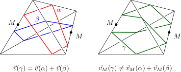
Figure 1: A length 8 curve that is not the sum of two length 4 curves in the marked triangulation.

Here $M$-normal curve theory differs from standard normal curve theory. While all normal curves are compatible, $M$-normal curves have distinct compatibility classes, and this increases the number of fundamentals. In Figure 1, we see the boundary of a tetrahedron with two marked points, one on each of a pair of opposite edges. Let $\gamma$ be the length 8 $M$-normal curve that meets each of the sub-edges once. As a normal curve $\gamma$ is not fundamental—it is the sum of the two distinct length 4 curves $\alpha$ and $\beta$. But in the marked triangulation these curves are incompatible and $\gamma$ is fundamental.

If $\alpha$ is an (almost) $M$-normal curve or surface, then $\vec{v}_{M}(\alpha)$ is a solution to a set of matching equations: For a triangulated surface, this set consists of one equation for each sub-edge in the interior of the surface. It sets equal the sum of those coordinates meeting the sub-edge from one side to the sum of those meeting it on the other side. In a triangulated 3-manifold, the set of matching equations consists of one equation for each $M$-normal arc type contained in an interior face. This equation sets equal the sum of the coordinates for elementary types using the arc type on one side to the sum of those using it on the other side.

We say that a vector $\vec{v}_{M}$ of the correct dimension is $M$-admissible if all its coordinates are non-negative, it satisfies the matching equations, and is self-compatible, i.e., it does not possess non-zero coordinates for any pair of non-$M$-compatible types. If $\vec{v}_{M}$ is an $M$-admissible vector, there is an (almost) $M$-normal curve/surface $\alpha$ for which $\vec{v}_{M}=\vec{v}_{M}(\alpha)$.

The following proposition is a straightforward generalization of a well known fact from normal surface theory to $M$-normal surfaces; see [HLP99] for a nice exposition.

Proposition 5.2.

Given a $3$-manifold with a marked triangulation $\mathcal{T}_{M}$, the set $\mathcal{F}$ of fundamental $M$-normal surfaces is computable, and both $|\mathcal{F}|$ and the maximum weight $\operatorname{wt}(F)$ of an $F\in\mathcal{F}$ are bounded by a computable function of $t$ and $m$.

The bound on $|\mathcal{F}|$ and $\operatorname{wt}(F)$ has the form $\exp(p(t,m))$, where $p(t,m)$ is a suitable polynomial.

Proof.

It is well known that without the marking, there are $7t$ normal disk types, $3t$ exceptional octagons and $25t$ exceptional tubed pairs of disks. Moreover, the presence of a tubed pair of disks may split one type of normal disks into two, but certainly we have no more than $42t$ types in total.

The points of $M$ divide each edge into at most $m+1$ subarcs. In order to specify an $M$-normal type of a triangle, for example, we need to specify the subarc containing each of the three vertices, which leads to the bound $(m+1)^{3}$. The worst bound is obtained for tubes and octagons, with $(m+1)^{8}$, so a rough bound for the total number of $M$-types is $42t(m+1)^{8}$.

A similar way of counting applies to the number of matching equations, which represent compatibility of the coordinates of the $M$-normal vector across the pieces of the edges of $\mathcal{T}$ delimited by the points of $M$. Indeed, the matching equations correspond to $M$-arc types. There are at most $4t$ interior faces, each with $3$ underlying normal arc types. A given $M$-arc type is thus determined by this normal type and by the sub-arcs it meets, and so there are at most $12t(m+1)^{2}$ matching equations.

Then, reasoning as in [HLP99, Sec. 6], using a Hilbert basis of the appropriate integral cone, we obtain the bounds of the claimed form. ∎

5.1 Snug pairs of curves and surfaces, Haken sums, and normal sums

The normal sum $F+G$ of a pair of (almost) $M$-normal curves or surfaces $F$ and $G$ has been defined, if they are $M$-compatible, to be an $M$-normal surface whose $M$-normal vector is the sum of the $M$-normal vectors of $F$ and $G$, $\vec{v}_{M}(F+G)=\vec{v}_{M}(F)+\vec{v}_{M}(G)$.

It is desirable to show that qualities of the sum, such as essentiality or minimality, also apply to the summands. Here we describe a well known geometric interpretation of the sum that makes this possible; also see, for example, [JO84, JT95]. We also present some related material.

Snug pairs. We begin with a definition of a “placement with no unnecessary intersections” for a pair of curves or surfaces.

Definition 5.3.

A pair $(F,G)$ of properly embedded curves or surfaces is snug if it is transverse and the number of components of the intersection $F\cap G$ is minimized over pairs $(F^{\prime},G^{\prime})$, where $F^{\prime}$ and $G^{\prime}$ are isotopic to $F$ and $G$, respectively. The pair $(F,G)$ is locally snug if $F\cap G$ is disjoint from the 1-skeleton $\mathcal{T}^{1}$, and, they are snug in the interior of each simplex of the triangulation (here we only allow isotopies moving each intersection of $F$ or $G$ with a face only within that face).

If $F$ and $G$ are locally snug $M$-normal surfaces then it follows that:

1. each pair of $M$-normal arcs, one from $F$ and one from $G$, meets in 0 or 1 points;

2. each pair of $M$-normal disks, one from $F$ and one from $G$, meets in 2 or fewer arcs, and the union of the arcs has at most one endpoint in any face;

3. no loop of $F\cap G$ lies inside a tetrahedron.

Any pair of compatible $M$-normal curves or surfaces can be made locally snug by $M$-normal isotopies that first make their intersections with edges disjoint and then “straighten” them so that: normal arcs are straight, normal triangles are flat, and normal quads are the union of two flat triangles. We do not define locally snug when $F$ is an almost normal surface and $G$ is a normal surface, for in that case we require only the definition of the normal sum $F+G$ and not its geometric interpretation.

Haken sum and normal sum of curves. Now, for a while, we deal only with curves, and we develop a geometric interpretation of their normal sum. Here we consider only unmarked triangulations, i.e., $M=\emptyset$.

Let $D$ be a regular neighborhood of an intersection point $x$ of a pair of transverse curves $\alpha$ and $\beta$. We can remove the intersection by deleting the arcs in the interior of the disk and then attaching $\alpha$ to $\beta$ along a pair of antipodal sub-arcs of $\partial D$. Thus, we replace the “$\times$” in $\alpha\cup\beta$ with either “$)($” or “$\asymp$”. This is called an exchange or a switch at $x$. A curve is said to be a Haken sum $\alpha~{}\widetilde{+}~{}\beta$ of $\alpha$ and $\beta$ if it is obtained by an exchange at each of their intersection points. Of course, $\alpha~{}\widetilde{+}~{}\beta$ is dependent on the direction of the switches and is therefore not well determined.

If, however, $\alpha$ and $\beta$ are locally snug normal curves, then each intersection point is of the form $x=\alpha^{\prime}\cap\beta^{\prime}$ where $\alpha^{\prime}$ and $\beta^{\prime}$ are normal arcs in some face. Then $\alpha^{\prime}$ and $\beta^{\prime}$ meet at least one common edge $e$ of the face. The regular exchange is the exchange that does not produce an abnormal arc, a non-normal arc with both endpoints attached to $e$; see Fig. 2 top.

Figure 2: Switches for curves and surfaces

As we will see, the normal sum of $\alpha+\beta$ of locally snug curves can be obtained by doing all the regular exchanges.

Lemma 5.4.

Let $\alpha$ and $\beta$ be locally snug normal curves. Then the Haken sum $\alpha~{}\widetilde{+}~{}\beta$ obtained by making all the regular exchanges is the normal sum $\alpha+\beta$; i.e., $\vec{v}(\alpha+\beta)=\vec{v}(\alpha)+\vec{v}(\beta)$.

Proof.

We show that the result holds in each face of the triangulation. In an abuse of notation, let $\alpha$ and $\beta$ be restriction of the curves to a particular face. For contradiction suppose that they are a counterexample that minimizes $|\alpha\cap\beta|$. Then $\alpha$ and $\beta$ are not disjoint, for in that case, the union is normal and normal vectors add.

Since they intersect in a face, we can identify an outermost half-bigon bounded by a sub-arcs of $\alpha$ and $\beta$ and an edge of the face; see Figure 3. The regular exchange trades these sub-arcs and results in a pair of normal curves, $\alpha^{\prime}$ normally isotopic to $\alpha$ and $\beta^{\prime}$ normally isotopic to $\beta$, that are locally snug but with fewer intersections. By assumption, these $\alpha^{\prime}$ and $\beta^{\prime}$ satisfy the conclusion, hence so do $\alpha$ and $\beta$. ∎

Lemma 5.5.

Let $\alpha~{}\widetilde{+}~{}\beta$ be a Haken sum of locally snug properly embedded curves. Then $\alpha~{}\widetilde{+}~{}\beta$ is normal if and only if $\alpha$ and $\beta$ are normal and all switches are regular, i.e., $\alpha~{}\widetilde{+}~{}\beta=\alpha+\beta$. In addition, if $\alpha$ and $\beta$ are normal and $\alpha~{}\widetilde{+}~{}\beta$ contains at least one irregular switch, then $\alpha~{}\widetilde{+}~{}\beta$ contains an abnormal arc.

Proof.

($\Leftarrow$) This is by Lemma 5.4. ($\Rightarrow$) We show that if either $\alpha$ or $\beta$ is not normal then neither is $\alpha~{}\widetilde{+}~{}\beta$ for any Haken sum of the curves.

Suppose then that $\alpha^{\prime}\subset\alpha$ is an outermost non-normal arc, one that co-bounds a disk with a sub-arc of an edge $e^{\prime}\subset e$. If $\beta$ meets the disk, it meets it in a collection of $n$ arcs, each with one endpoint in $\alpha^{\prime}$ and one endpoint in $e^{\prime}$, because $\alpha^{\prime}$ is outermost and $\alpha$ and $\beta$ are snug. Let $D$ be a regular neighborhood of the disk. Then, regardless of the switches, $\alpha~{}\widetilde{+}~{}\beta$ meets $D$ in a collection of $n+1$ arcs that have $n+2$ endpoints along the edge and $n$ endpoints not on the edge. It follows that at least one arc meets the edge in 2 points and is not normal. A symmetric argument applies if the outermost non-normal arc belongs to $\beta$. Nor can either $\alpha$ or $\beta$ possess a loop in a face. Local snugness implies that any loop is disjoint from the other curve and survives any Haken sum.

We now know that $\alpha$, $\beta$ are normal. To conclude the proof, it is sufficient to show that $\alpha~{}\widetilde{+}~{}\beta$ contains an abnormal arc if at least one switch is irregular (this contradicts the normality of $\alpha+\beta$, and thus proves the last claim of the lemma). In an abuse of notation, let $\alpha$ and $\beta$ refer to the collection of normal arcs in a particular face.

We perform the specified switches in order according to the following scheme: If $\alpha\cap\beta\neq\emptyset$, then $\alpha$ and $\beta$ form an outermost half bigon $B$ with an edge as in Figure 3. The regular switch produces collections $\alpha^{\prime}$ and $\beta^{\prime}$ that are normally isotopic to $\alpha$ and $\beta$, but with one fewer intersections. An irregular switch produces a disjoint abnormal arc that survives any and all additional exchanges. If each exchange is regular, we can continue and the process produces a disjoint union $\alpha\sqcup\beta.$ If any exchange is not regular, the resulting curve contains an abnormal arc. ∎

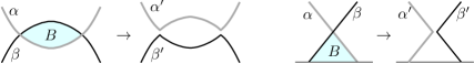
Figure 3: Exchanges at the corners of a bigon and a half-bigon.

Normal sign. When $\alpha$ and $\beta$ lie in an oriented surface, for example the boundary of an oriented manifold, we can define the normal sign of each point of $\alpha\cap\beta$. Viewing $\alpha$ as horizontal and $\beta$ as vertical, the regular exchange at the point connects a pair of quadrants. The point has positive sign if the exchange connects the southwest quadrant to the northeast quadrant, and it has negative sign if it connects the northwest to the southeast; see Figure 4. This is equivalent to the definition given in [BDTS12]. The definition depends on the ordering of the pair of curves and on an orientation on the surface: reversing the order or the orientation reverses every sign.

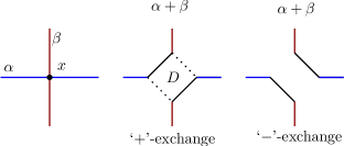
Figure 4: Exchanges with positive and negative sign.

Normal sum of surfaces. Similar to the case of curves above, one can also construct the normal sum $F+G$ of normal surfaces geometrically, using suitable switches. We assume that $F$ and $G$ are locally snug.

We construct $F+G$ by specifying its intersection with the 1-, 2-, and 3-skeleta of the triangulation, respectively. First, we let the intersection of $F+G$ with the 1-skeleton to be the union of the intersection points from $F$ and those from $G$.

Second, in each face we perform regular switches on all intersecting pairs of arcs $(f,g)$, where $f$ comes from $F$ and $g$ from $G$.

Finally, we construct the normal sum $F+G$ in the interior of each tetrahedron $T$. As discussed earlier, each normal disk is either a flat triangle or a quadrilateral made of 2 flat triangles. It follows that every intersection between normal disks from compatible surfaces is either 1 or 2 arcs, not necessarily straight. Compatibility ensures that the regular switches prescribed at the endpoints of each arc are consistent with each other and can be extended across the entire arc of intersection. The normal sum $F$ and $G$ is the result of performing such regular switches along every such arc of intersection.

Note that any intersection arc between normal disks can be extended from a tetrahedron through a face to a neighboring tetrahedron. In its entirety this intersection curve between $F$ and $G$ is either a loop, or an arc with both endpoints in $\partial X$. Compatibility ensures that the regular switches in each face and through the interior of each tetrahedron agree. Thus we can regard the switch as a regular switch along the entire intersection curve.

Exchange arcs and surfaces, trace curves. Here we introduce some additional terminology. First, we consider a regular switch of two curves. Inside the neighborhood where the regular switch was performed, we identify an exchange arc that connects the points of the newly formed arcs corresponding to the former intersection points; see Figure 2.

Next, we consider two locally snug normal surfaces $F$ and $G$. A patch is a component of $F\cup G\setminus F\cap G$. Regular switches reconnect the patches, and trace curves are the seams between patches after performing regular switches along all intersection curves; see Figures 2 and 5.

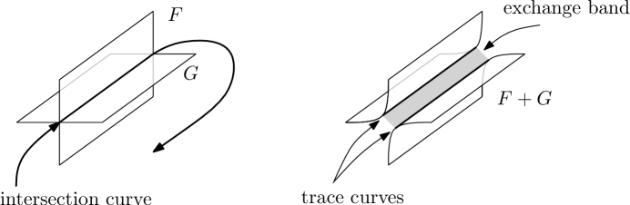
Figure 5: The exchange between surfaces along an intersection curve.

If the intersection curve $\alpha$ is an arc, then, after performing a regular switch, we can identify an exchange rectangle, a rectangle whose top and bottom, say, are bounded by trace arcs and whose left and right sides are exchange arcs lying in $\partial X$.

If $\alpha$ is a loop, then our assumption that $X$ is orientable means that a regular neighborhood of $\alpha$ is a solid torus, not a solid Klein bottle. Again, since $X$ is orientable, $\alpha$ is either orientation preserving in both $F$ and $G$, or, orientation reversing in both $F$ and $G$. In the former case, there is an exchange annulus, a zero-weight annulus bounded by the trace curves and with core $\alpha$. In the latter case, there is a single trace curve which bounds an exchange Möbius band (we will be able to exclude this case in our proofs, though).

As observed in [Hat82] and, in the context of normal surfaces, in [JS03], every intersection arc between surfaces connects intersection points of the boundary curves that have opposite normal sign:

Lemma 5.6.

Let $A=B+C$ be a normal sum of surfaces in an orientable manifold $X$ with an induced orientation on $\partial X$. Then every arc in $B\cap C$ joins a pair of points in $\partial B\cap\partial C$ with opposite normal sign.

6 Complexity and tight curves

In this section, we consider properly properly embedded curves in a triangulated surface. We assume that they are transverse to the 1-skeleton but, a priori, they are not assumed to be normal.

Fix, once and for all, an ordering of all normal arc types of the triangulated surface. For this purpose we do not take into account any marking present. As in the previous section, a normal curve $\alpha$ determines a vector $\vec{v}(\alpha)$ which records the number of normal arcs of the indexed type. Order these normal vectors lexicographically.

Recall that the length of a properly embedded curve $\alpha$ is the number of intersections with the 1-skeleton, $\ell(\alpha)=|\alpha\cap\mathcal{T}^{1}|$. We say that a curve is least length if it minimizes length over all curves to which it is isotopic.

Lemma 6.1.

A least length essential curve is normal.

Proof.

A loop in face demonstrates that the curve is not essential and any abnormal arc is either inessential or yields an isotopy reducing the length. ∎

If $\alpha$ is a normal curve, then we define its complexity to be the pair consisting of its length and its normal vector,

$$\operatorname{cpx}(\alpha):=(\ell(\alpha),\vec{v}(\alpha)).$$

We reiterate that we do not take into account any marking $M$ in the definition of complexity. If $\alpha$ is not normal, we define its complexity to be $\operatorname{cpx}(\alpha)=(\ell(\alpha),\vec{0})$. Complexities will also be ordered lexicographically.

Definition 6.2.

A curve $\alpha$ is tight if it minimizes the complexity $\operatorname{cpx}(\alpha)$ over all curves to which it is isotopic.

The interior of a connected inessential curve can be made disjoint from the 1-skeleton, so a tight inessential loop has $\operatorname{cpx}=(0,\vec{0})$ and a tight inessential arc has $\operatorname{cpx}=(2,\vec{0})$.

Lemma 6.3.

A tight essential curve is normal and unique up to normal isotopy.

Proof.

Indeed, the complexities of two normal curves are equal if and only if their normal vectors are identical. ∎

Lemma 6.4.

Let $\alpha~{}\widetilde{+}~{}\beta$ be a Haken sum of locally snug properly embedded curves. Then $\operatorname{cpx}(\alpha~{}\widetilde{+}~{}\beta)\leq\operatorname{cpx}(\alpha)+\operatorname{cpx}(\beta)$ with equality holding if and only if $\alpha,\beta$ and $\alpha~{}\widetilde{+}~{}\beta$ are all normal, or, all not normal.

Proof.

The curve $\alpha~{}\widetilde{+}~{}\beta$ is constructed by performing an exchange at every intersection point of $\alpha\cup\beta$. This is done away from the 1-skeleton, so we have $\ell(\alpha~{}\widetilde{+}~{}\beta)=\ell(\alpha)+\ell(\beta)$. Thus any difference in complexity is determined solely by the normal vectors of the curves. If $\alpha~{}\widetilde{+}~{}\beta$ is normal, then by the previous two lemmas $\vec{v}(\alpha+\beta)=\vec{v}(\alpha)+\vec{v}(\beta)$ and equality holds. If $\alpha~{}\widetilde{+}~{}\beta$ is not normal, then its normal vector is $\vec{0}$. Then complexity is additive when both $\alpha$ or $\beta$ are not normal, and sub-additive otherwise. ∎

If a tight curve is written as a sum, then the exchange arcs are essential in the complement of the curve:

Lemma 6.5.

Suppose that a tight normal curve is written as a sum $\alpha+\beta$ of two normal curves. Then no exchange arc co-bounds a disk with a sub-arc of the curve.

Proof.

Perform an irregular exchange only at the intersection corresponding to this exchange arc. The new curve is a Haken sum $\alpha~{}\widetilde{+}~{}\beta$ with one component a trivial loop, the rest isotopic to $\alpha+\beta$, and the same total length. It follows that the trivial loop has zero length otherwise $\alpha+\beta$ would not be tight. Therefore $\alpha+\beta$ and the second component of $\alpha~{}\widetilde{+}~{}\beta$ are normally isotopic. However, by Lemma 5.5 there is an abnormal arc in the second component of $\alpha~{}\widetilde{+}~{}\beta$, a contradiction. ∎

Lemma 6.6.

Let $B$ be a bigon or half-bigon bounded by a pair of locally snug normal curves $\alpha$ and $\beta$; see Figure 3. Let $\alpha^{\prime}$ and $\beta^{\prime}$ be the pair of isotopic curves obtained by corner exchange(s) that trade the sides of $B$. Then one of the following holds:

1. $\operatorname{cpx}(\alpha^{\prime})=\operatorname{cpx}(\alpha),\operatorname{cpx}(\beta)=\operatorname{cpx}(\beta^{\prime})$, thus $\alpha^{\prime}$ and $\beta^{\prime}$ are normally isotopic to $\alpha$ and $\beta$, respectively, and $|\alpha^{\prime}\cap\beta^{\prime}|<|\alpha\cap\beta|$;

2. $\operatorname{cpx}(\alpha^{\prime})<\operatorname{cpx}(\alpha)$;

3. $\operatorname{cpx}(\beta^{\prime})<\operatorname{cpx}(\beta)$.

Proof.

Let $\alpha,\alpha^{\prime},\beta$ and $\beta^{\prime}$ be as indicated in Figure 3. Note that the exchange doesn’t add or remove intersections with the 1-skeleton, and so the total length is unchanged. If the traded arcs differ in length then one curve increases and the other decreases in length, hence in complexity. In this case, either (2) or (3) holds. So we continue assuming $\ell(\alpha)=\ell(\alpha^{\prime})$ and $\ell(\beta)=\ell(\beta^{\prime})$.

If any exchange is irregular, then one of the curves, say $\alpha^{\prime}$, is not normal. Then its complexity $\operatorname{cpx}(\alpha^{\prime})=(\ell(\alpha^{\prime}),\vec{0})=(\ell(\alpha),\vec{0})<(\ell(\alpha),\vec{v}(\alpha))=\operatorname{cpx}(\alpha)$ has decreased, yielding conclusion (2). Conclusion (3) results when $\beta^{\prime}$ is not normal.

We are left in the case that the exchange trades length fairly and $\alpha^{\prime}$ and $\beta^{\prime}$ are both normal. Because length and normal vectors are both additive with respect to normal addition, we have $\operatorname{cpx}(\alpha)+\operatorname{cpx}(\beta)=\operatorname{cpx}(\alpha+\beta)=\operatorname{cpx}(\alpha^{\prime})+\operatorname{cpx}(\beta^{\prime})$. If $\operatorname{cpx}(\alpha^{\prime})=\operatorname{cpx}(\alpha)$, then $\operatorname{cpx}(\beta^{\prime})=\operatorname{cpx}(\beta)$ and by Lemma 6.3 the trade yields normally isotopic curves, conclusion (1). Otherwise, either (2) or (3) holds. ∎

Lemma 6.7.

Let $\alpha$ be a tight essential curve and $\mathcal{C}$ set of pairwise snug, tight essential curves. Then, after a normal isotopy of $\alpha$, $\{\alpha\}\cup\mathcal{C}$ is pairwise snug.

Proof.

Normally isotope $\alpha$ to minimize the total of all intersections with $\mathcal{C}$. By way of contradiction, suppose some pair is not snug, that there is $\beta\in\mathcal{C}$ for which $|\alpha\cap\beta|>i(\alpha,\beta)$. Among all such $\beta$ take one that, together with $\alpha$, determines an innermost bigon; then any other curves from $\mathcal{C}$ meeting that bigon meet it in arcs that run straight across.

Apply Lemma 6.6. Since all curves are tight, we must have the first conclusion. But, trading across the bigon reduces intersections between $\alpha$ and $\beta$ without raising intersections of any other pair—a contradiction. ∎

Lemma 6.8.

Suppose that a tight essential normal curve is a normal sum $\alpha+\beta$. Then $\alpha$ and $\beta$ are tight, essential, and after a normal isotopy, snug.

Proof.

Normally isotope $\alpha$ and/or $\beta$ to minimize $|\alpha\cap\beta|$. This does not change their sum.

First we show that the pair is snug: If not, then some pair of sub-arcs of $\alpha$ and $\beta$ bound a bigon or half-bigon $B$. Apply Lemma 6.6. The first conclusion does not hold, so without loss of generality assume that $\operatorname{cpx}(\alpha^{\prime})<\operatorname{cpx}(\alpha)$. Isotope $\alpha^{\prime}$ back slightly so that $\alpha^{\prime}$ and $\beta$ still overlap and form a very thin bigon. Since $\alpha\cup\beta$ and $\alpha^{\prime}\cup\beta$ are isotopic as graphs, $\alpha+\beta$ is isotopic to some Haken sum $\alpha^{\prime}~{}\widetilde{+}~{}\beta$. But by Lemma 6.4, $\operatorname{cpx}(\alpha^{\prime}~{}\widetilde{+}~{}\beta)\leq\operatorname{cpx}(\alpha^{\prime})+\operatorname{cpx}(\beta)<\operatorname{cpx}(\alpha)+\operatorname{cpx}(\beta)=\operatorname{cpx}(\alpha+\beta)$, a contradiction.

It follows that $\alpha$ and $\beta$ are both essential. If either possesses a component that bounds a disk, then the fact that $\alpha$ and $\beta$ are snug implies that this component misses the other curve, survives normal addition, and $\alpha+\beta$ contains an inessential component, a contradiction.

It remains to show that each summand is tight. Without loss of generality, suppose that $\alpha$ is not tight, that there is a tight curve $\alpha_{t}$ with lower complexity, $\operatorname{cpx}(\alpha_{t})<\operatorname{cpx}(\alpha)$, that is isotopic to $\alpha$ but not normally so. Isotope $\alpha_{t}$ to intersect $\alpha\cup\beta$ minimally.

Then any innermost (half-) bigon in the complement of $\alpha_{t}\cup\alpha\cup\beta$ is bounded by $\alpha$ and $\alpha_{t}$, since it cannot be bounded by $\alpha$ and $\beta$, which are snug. And because any patch of $\beta$ is a sub-arc of $\alpha+\beta$, any innermost (half-) bigon bounded by $\beta$ and $\alpha_{t}$ is also a (half-) bigon bounded by the tight curves $\alpha+\beta$ and $\alpha_{t}$ which, using Lemma 6.6 again, can be eliminated by a normal isotopy of $\alpha_{t}$. This contradicts the minimality of the intersection between $\alpha_{t}$ and $\alpha\cup\beta$.

Then, sub-curves of $\alpha$ and $\alpha_{t}$ co-bound a product region $R$ as in Figure 6.

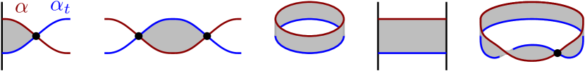
Figure 6: Possible product regions derived from isotopy of $\alpha$ and $\alpha_{t}$.

If they are not snug, $R$ is a bigon or half-bigon. If they are snug, $R$ is a rectangle when $\alpha$ is an arc, an annulus when $\alpha$ is a two-sided loop, and a bigon with corners identified when $\alpha$ is a one-sided loop.

In all of these cases, as observed above, no arc of $\beta$ forms a (half-) bigon inside $R$, and must therefore run across $R$ and have an endpoint in both $\alpha$ and $\alpha_{t}$.

In the non-snug case, let $\alpha^{\prime}$ be the curve of less complexity obtained by routing $\alpha$ along $\alpha_{t}$ when it meets the bigon or half-bigon. In the snug case, let $\alpha^{\prime}=\alpha_{t}$. In either case, $\operatorname{cpx}(\alpha^{\prime})<\operatorname{cpx}(\alpha)$. Moreover, the complex $\alpha^{\prime}\cup\beta$ is isotopic to $\alpha\cup\beta$ and because they are isotopic, there are exchanges, not necessarily regular, so that the Haken sum $\alpha^{\prime}~{}\widetilde{+}~{}\beta$ is a curve isotopic to $\alpha+\beta$. But by Lemma 6.4, $\operatorname{cpx}(\alpha^{\prime}~{}\widetilde{+}~{}\beta)\leq\operatorname{cpx}(\alpha^{\prime})+\operatorname{cpx}(\beta)<\operatorname{cpx}(\alpha)+\operatorname{cpx}(\beta)=\operatorname{cpx}(\alpha+\beta)$. This contradicts the fact that $\alpha+\beta$ is tight. ∎

Rails and fences. Now we again consider a triangulation with a marking $M$, and auxiliary curves in it that, unlike $M$-normal curves, go through the points of $M$.

A rail is a normal arc with its endpoints in $M$, and a fence is a normal curve that is the union of rails.

We note that if a face contains an $M$-normal arc $\alpha$ and a rail $\mu$ that are locally snug, then $|\alpha\cap\mu|$ is either $0$ or $1$, depending only on the endpoints of $\mu$ and the $M$-normal type of $\alpha$.

The following lemma can also be considered obvious:

Lemma 6.9.

Intersection number with fences is additive with respect to normal addition of $M$-normal curves: If $\mu$ is an fence and $\alpha$ and $\beta$ are $M$-compatible, $M$-normal curves, then $|(\alpha+\beta)\cap\mu|=|\alpha\cap\mu|+|\beta\cap\mu|.$

Proposition 6.10.

Let $\mu$ be a fence that is a tight essential curve (w.r.t. the unmarked triangulation). Suppose that a sum $\alpha+\beta$ of $M$-normal curves is tight, essential and snug with $\mu$. Then

1. $\alpha$ and $\beta$ are both snug with respect to $\mu$;

2. $i(\alpha+\beta,\mu)=i(\alpha,\mu)+i(\beta,\mu)$ where $i(.,.)$ is the geometric intersection number;

3. if $\beta$ is two-sided, connected and normally isotopic to $\mu$ then, after a normal isotopy, every point of $\alpha\cap\beta$ has the same normal sign.

Proof.

Among counterexamples to conclusion (1) of the proposition, choose one that minimizes $|\alpha\cap\beta|$. Then $\alpha,\beta$ and $\mu$ are pairwise locally snug, and we will show that they are in fact pairwise snug. Suppose not and let $B$ be an innermost (half-) bigon bounded by some pair of the curves.

If $B$ is bounded by $\mu$ and either of the other curves, say $\alpha$, then every sub-arc of $\beta$ in $B$ crosses $B$ and meets both $\alpha$ and $\mu$. Let $\alpha^{\prime}$ be the result of rerouting $\alpha$ around $B$ as in Lemma 6.6. Then $\alpha+\beta$ is isotopic to some Haken sum $\alpha^{\prime}~{}\widetilde{+}~{}\beta$ that has fewer intersections with $\mu$. This contradicts our assumption that $\alpha+\beta$ and $\mu$ are snug.

If $B$ is bounded by $\alpha$ and $\beta$, then every sub-arc of $\mu$ in $B$ crosses $B$ and meets both $\alpha$ and $\beta$. Let $\alpha^{\prime}$ and $\beta^{\prime}$ be the curves given by Lemma 6.6. Because $\alpha+\beta$ is tight, $\alpha$ and $\beta$ are tight and normally, but not necessarily $M$-normally, isotopic to $\alpha^{\prime}$ and $\beta^{\prime}$, respectively. Because the normal sum $\alpha+\beta$ was defined, $\alpha$ and $\beta$ are locally snug. The isotopy doesn’t create intersections, and so $\alpha^{\prime}$ and $\beta^{\prime}$ are also locally snug. Then $\alpha+\beta=\alpha^{\prime}~{}\widetilde{+}~{}\beta^{\prime}$ for some generalized Haken sum of $\alpha^{\prime}$ and $\beta^{\prime}$. By Lemma 5.5 that sum is a normal sum, $\alpha+\beta=\alpha^{\prime}+\beta^{\prime}$. Note that $\alpha^{\prime}$ and $\beta^{\prime}$ are snug with $\mu$ if and only if $\alpha$ and $\beta$ are, as the move did not change the number of times they meet $\mu$. Since $|\alpha\cap\beta|>|\alpha^{\prime}\cap\beta^{\prime}|$ we obtain a contradiction and establish conclusion (1).

Since $\alpha$, $\beta$ and their sum are all snug with respect to $\mu$ and intersections with respect to $\mu$ are additive, we have additivity of geometric intersection number, conclusion (2).

We now prove the final statement of the proposition. Assume that $\beta$ is normally isotopic to $\mu$. Then $i(\beta,\mu)=0$ since $\beta$ is two-sided. By (2) and the fact that $\alpha+\beta$ and $\alpha$ are both snug with $\mu$ we have: $|(\alpha+\beta)\cap\mu|=i(\alpha+\beta,\mu)=i(\alpha,\mu)=|\alpha\cap\mu|$.

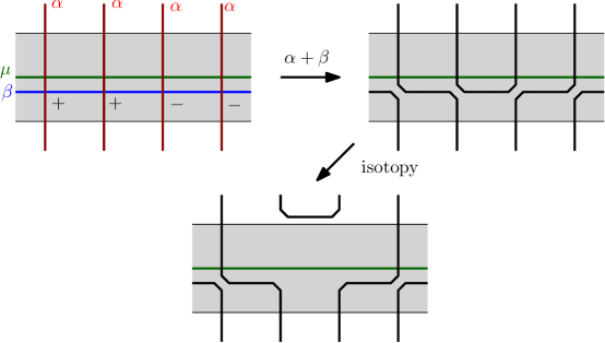
Figure 7: Mixed normal signs imply that $i(\alpha+\beta,\beta)<i(\alpha,\beta)$.

And since $\beta$ is normally isotopic to $\mu$, there is a normal, not necessarily $M$-normal, isotopy taking $\alpha+\beta$ to $\alpha+\mu$. Now $\alpha$ cuts across a thin regular neighborhood of $\mu$ in a collection of arcs that span (cut across) the neighborhood. Together they cut this neighborhood into rectangles; see Figure 7.

Each regular exchange connects a pair of rectangles at a corner of each. In fact, every rectangle that meets $\alpha\cap\mu$ twice must be attached to another rectangle at one of its corners. Otherwise, an arc of $\alpha+\mu$ bounds the unattached rectangle, showing that the arc it is trivial in the neighborhood of $\mu$ and can be isotoped out of it. This would imply $i(\alpha+\beta,\mu)<|\alpha\cap\mu|$, contradicting the equality shown earlier. The fact that each rectangle is attached at exactly one corner implies that as we follow $\mu$ every intersection with $\alpha$ must have the same normal sign. Since $\beta$ is normally isotopic to $\mu$ we have our desired conclusion (3). ∎

7 Normal summands of incompressible annuli

We would like to apply two well known results from normal surface theory: (1) an essential surface is isotopic to a normal surface, and (2) every summand of a least weight essential normal surface is also least weight and essential (Theorem 6.5 of Jaco and Tollefson [JT95]). But, as will be seen shortly, our notion of surface complexity prioritizes the reduction of boundary complexity over the reduction of total surface weight. Thus the results (1) and (2) cannot be applied as stated.

Proposition 7.1 recovers the first result using our notion of complexity. Proposition 7.2 gives a weaker version of the second for incompressible annuli. While we expect the full version to hold with our notion of complexity, we prove a restricted version both to simplify the proof and to incorporate boundary parallel annuli which are non-essential. Our proof follows the strategy of [JO84] and [JT95].

The complexity $\operatorname{cpx}(F)$ of a properly embedded surface $F$ is the triple

$$\operatorname{cpx}(F)=(\operatorname{cpx}(\partial F),|F\cap\mathcal{T}^{1}|,|F\cap\mathcal{T}^{2}|)=((\ell(\partial F),\vec{v}(\partial F)),|F\cap\mathcal{T}^{1}|,|F\cap\mathcal{T}^{2}|).$$

We compare complexities lexicographically. Thus, the complexity of $F$ is measured first by the complexity of its boundary, then by the weight of $F$, $\operatorname{wt}(F)=|F\cap\mathcal{T}^{1}|$, and then by the number of components of the intersections with the $2$-skeleton of $\mathcal{T}$.

A normal surface is least complexity if it minimizes complexity among normal surfaces to which it is isotopic (but not necessarily normally isotopic).

A surface is tight if it minimizes complexity, ranging over all those surfaces to which it is isotopic.

A tight normal surface is clearly least complexity, and as a consequence of Proposition 7.1, a normal essential surface of least complexity is tight. But, this does not hold in general for surfaces that are not essential: for example, a normal boundary parallel annulus may be least complexity but after tightening no longer normal.

We first recover normalization of an essential surface. We will apply this with surfaces whose boundaries are tight, hence least length.

Proposition 7.1.

Suppose that $X$ is a triangulated, irreducible manifold with incompressible boundary. If $F\subset X$ is a tight, properly embedded, essential surface, then $F$ is normal.

Proof.

To prove $F$ is normal we must show that it meets each tetrahedron $\Delta$ in a collection of disks whose boundaries are normal curves of length 3 or 4. We adopt the view taken in [BDTS12], showing $F$ meets each tetrahedron in pieces that are incompressible and edge incompressible.

If any component of $F\cap\Delta$ is compressible in $\Delta$, then, by an innermost disk argument, we obtain a compressing disk avoiding all other components of $F\cap\Delta$, and hence $F\cap\Delta$ is compressible inside $\Delta$.

Because $F$ is essential, the boundary of any compressing disk $D$ for $F\cap\Delta$ is trivial in $F$. Because $X$ is irreducible, compressing along $D$ yields a surface $F^{\prime}$ that is isotopic to $F$, but for which either $|F\cap\mathcal{T}^{1}|$ or $|F\cap\mathcal{T}^{2}|$ has been reduced, a contradiction. It follows that $F\cap\Delta$ is the union of disks.

An edge compressing disk for a surface in $\Delta$ is an embedded disk $E$ whose boundary $\partial E=e\cup f$, consists of two arcs, $e\subset\mathcal{T}^{1}$ and $f=E\cap F=\partial E\cap F$; see [BDTS12].

If some component of $F\cap\Delta$ has an edge compressing disk then, by an innermost disk argument, there is an edge compressing disk $E$ for $F\cap\Delta$. If $e\subset\partial X$ then, because $F$ is not boundary compressible, $f$ is trivial in $F$. But compressing along $E$ yields an isotopic surface $F_{0}$ ($X$ is irreducible and has incompressible boundary) whose boundary length is reduced by at least two, contradicting the fact that $\partial F=\partial F_{0}$ is least length. And if $e$ lies in an interior edge, then $E$ can be used to guide an isotopy reducing $|F\cap\mathcal{T}^{1}|$, also a contradiction.

Then $F$ meets each face in normal arcs. For otherwise, there is an arc whose ends both lie in the same edge, and an outermost such arc bounds an edge compressing disk. Then $F$ meets the boundary of each tetrahedron in normal curves. And it is well known, see Thompson [Tho94], that if any such curve has length greater than 4 we see an edge compressing disk for $F$ in the boundary of the tetrahedron. ∎

0-efficient triangulations. First we recall the definition of $0$-efficient triangulations from [JR03]. A triangulation of a manifold $X$ with nonempty boundary is $0$-efficient if every normal disk is vertex-linking. (A normal disk is vertex-linking at vertex $v$ if it consists of precisely one normal triangle from each tetrahedral corner meeting $v$.)

Moreover, if no boundary component of $X$ is an $S^{2}$, then $X$ does not contain any normal $2$-spheres [JR03, Prop. 5.15]. In our setting, we use $0$-efficient triangulations only in the situations without $S^{2}$ boundary components (since in the algorithm, we fill each such component with a ball). Note also that in the proposition below we can assume that $X$ does not contain $S^{2}$ boundary components even if do not explicitly claim that $X$ is obtained in an intermediate stage of the algorithm. Indeed, we assume that $X$ is irreducible. Then an $S^{2}$ boundary component implies that $X$ is a ball; however, the proposition also assumes that $X$ contains an essential annulus or Möbius band.

We now establish the second result, that some summand of a non-fundamental incompressible annulus is an essential annulus. This applies to boundary compressible as well as essential annuli.

Proposition 7.2.

Let $X$ be a triangulated, orientable, irreducible manifold with incompressible boundary and a $0$-efficient triangulation. Let $A$ be an incompressible annulus or Möbius band that has tight boundary and is least complexity and normal. Suppose that $A$ can be written as a non-trivial sum $A=B+C$ where $B$ is connected and $\partial B\neq\emptyset$. Then $B$ is an essential annulus or Möbius band with tight boundary.

7.1 Proof of Proposition 7.2

Sketch of the proof. Our proof is loosely modeled on Jaco and Tollefson’s proof of [JT95, Th. 6.5]. Apart from using slightly different notion of complexity, we also have to add additional ingredients when $A$ is a boundary parallel annulus.

As we will see, the core of the proof is to show that $B$ is essential. For contradiction we assume that $B$ is not essential. The first important step is to find out what are the possible patches when $A$ is decomposed by trace curves from the normal sum $A=B+C$; see Figure 8 left. If $A$ is essential (annulus or Möbius band), then disk patches as well as half-disk patches can be ruled out following [JT95] (disk patches avoid $\partial X$ whereas half-disk patches contain a single arc on $\partial X$); see Lemmas 7.8 and 7.9. After ruling out such patches we can deduce that every intersection curve is essential in $B$, that is a spanning arc or a core curve. This already mean that $C$ intersects $B$ in a very specific way and both cases can be ruled out along [JT95]; see Lemma 7.11.

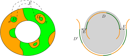
Figure 8: The annulus $A$ separated by trace curves into patches (left); $E$ is an exchange annulus. The right part shows a cross-section of $D\cup E\cup D^{\prime}$ assuming that $D$ and $D^{\prime}$ are not adjacent across $E$. Then $D\cup E\cup D^{\prime}$ separates, after a slight isotopy, two components of $A$.

If $A$ is not essential, then $A$ is a boundary parallel annulus by Proposition 4.2. In this case we do not know how to rule out disk patches but we still can rule out half-disk patches (Lemma 7.9); here we use that simplification of the boundary has higher priority than simplification of the interior in our notion of complexity. Since $A$ is boundary parallel, there is an annulus $A_{\partial X}$ to which $A$ is parallel and together they bound a solid torus $T$ in $X$. Because there are no half-disk patches, we can show that one of the exchange rectangles for the sum $A=B+C$ is inside this torus and it meets $A$ and $A_{\partial X}$ only in essential arcs. However, with such a rectangle $A$ cannot be boundary parallel; see Lemma 7.10 for details. This finishes the sketch of the proof and now we provide the details.

Because $A$ is incompressible, $\partial A$ is essential by Proposition 4.2. Without loss of generality, we will assume that the sum $A=B+C$ lexicographically minimizes $(|\partial B\cap\partial C|,|B\cap C|)$, the number of boundary intersections and the total number of intersection curves, over pairs $(B^{\prime},C^{\prime})$ where $B^{\prime}$ and $C^{\prime}$ are locally snug surfaces isotopic to $B$ and $C$, respectively. Since $\partial A(=\partial B+\partial C)$ is assumed tight, we have, by Lemma 6.8, that $\partial B$ and $\partial C$ are tight, and because $|\partial B\cap\partial C|$ is minimized, snug.

Lemma 7.3.

Either the conclusion of Proposition 7.2 holds, or $B$ is a boundary parallel annulus and every component of $C$ is an incompressible annulus, Möbius band, torus or Klein bottle.

Proof.

No component of $C$ has Euler characteristic $\chi>0$: Because $X$ is 0-efficient, no normal surface is a sphere, nor a projective plane, for then its normal double would be a normal sphere. And, also by 0-efficiency, any disk has boundary a trivial vertex linking curve that survives normal addition, and is present in $\partial A$—a contradiction.

Then every component has $\chi=0$ and it is an annulus, Möbius band, torus, or Klein bottle. No component is a compressible annulus since these have a trivial boundary component (Proposition 4.2) and this contradicts the fact that both summands have essential boundary.

Since $B$ is connected and $\partial B\neq\emptyset$, $B$ is either an annulus or Möbius band. Also by Proposition 4.2, a Möbius band is essential and satisfies the conclusion of Proposition 7.2. So does an annulus, unless it is boundary compressible, and hence boundary parallel, by Proposition 4.2. ∎

We proceed with the proof of Proposition 7.2 under the assumption that $B$ is a boundary parallel annulus.

When $A$ is formed as the normal sum $B+C$, it is partitioned into patches coming from $B$ and $C$, as was discussed in Section 5.1, and we have exchange surfaces attached to the curves separating the patches; see Figure 8 left.

It follows that no exchange surface is a Möbius band. As noted in Section 5.1, this occurs only when an intersection loop is one-sided in both summands.

Define a half disk to be a disk that is halfway properly embedded in $X$, that is, an embedded disk whose boundary meets $\partial X$ in a single arc. Note that a boundary compressing disk for a surface is a half disk whose boundary meets the surface in the complementary arc, but the reverse does not hold in general, for the arc may not be essential in the surface.

An exchange rectangle or annulus $E$ meets four patches of $A$. A pair $D,D^{\prime}$ of these patches are said to be adjacent across $E$ if they meet opposite boundary curves $\sigma$ and $\tau$ of $E$, but from the same side (we again refer to Figure 8 left).

Lemma 7.4.

$\sigma$ bounds (half) disk in $A$ if and only if $\tau$ both bounds a (half) disk in $A$.

Proof.

We prove that if $\sigma$ bounds a (half) disk in $A$, then $\tau$ bounds a (half) disk in $A$. The reverse implication is proved by interchanging $B$ and $C$ and remarking that in this proof we do not use the extra assumptions on $B$.

The surface $A$ is either essential or a boundary parallel annulus, and it is incompressible by the assumptions.

Suppose that $\sigma$ bounds a disk $D$ in $A$. Then $E\cup D$ is a disk which, after a slight isotopy, meets $A$ only in $\tau$. Since $A$ is incompressible, $\tau$ bounds a disk in $A$ as claimed.

The same argument works when $A$ is essential and, say, $\sigma$ bounds a half disk $H$. Then $E\cup H$ is a half disk which, after a slight isotopy, meets $A$ only in $\tau$. Since $A$ is not boundary compressible, $\tau$ bounds a half disk in $A$.

We conclude by showing that $\tau$ bounds a half disk when $\sigma$ bounds a half disk and $A$ is a boundary parallel annulus (assumed to have tight boundary). To obtain a contradiction, suppose that $\sigma$ bounds a half disk $H$ but $\tau$ is an essential arc in $A$. Then $E\cup H$ is, after a slight isotopy, a boundary compressing disk meeting $A$ in the arc $\tau$. Since $A$ is parallel to an annulus $A_{\partial X}\subset\partial X$, their union bounds a solid torus in $X$. The rectangle $E$ is a disk properly embedded in this solid torus.

Indeed, if $E$ is outside the solid torus, consider a boundary compressing disk $D_{A}$ for $A$ meeting $A$ in $\tau$ inside the solid torus. Then the disk $D_{A}\cup E\cup H$ meets the core curve of $A_{\partial X}$ exactly once, implying that it is a non-separating disk and therefore a compressing disk for $\partial X$—a contradiction.

As soon as we know that $E$ is inside the solid torus, we have that the boundary of $E$ meets $A_{\partial X}$ in a pair of exchange arcs that each span $A_{\partial X}$ by Lemma 6.5, and meets the annulus $A$ in one curve $\sigma$ that is trivial in $A$ and the other $\tau$ that is a spanning arc for $A$. Therefore, when restricting to $A_{\partial X}$, we get that two corners of $E$ are in one component of $\partial A$ and the other two in the second one. When restricting to $A$, we get that three corners are in the same component and the other corner in the second—a contradiction. ∎

Lemma 7.5.

Suppose $A$ is essential. If $\sigma$ and $\tau$ bound disks in $A$, then they are adjacent across $E$.

Proof.

Suppose that $\sigma$ and $\tau$ bound non-adjacent disks $D$ and $D^{\prime}$. They either are disjoint, or one is a sub-disk of the other, say $D^{\prime}\subset D$.

When disjoint, the union $D\cup E\cup D^{\prime}$ is a sphere that, after a slight isotopy, separates components of $A$ (since spheres separate in irreducible manifolds)—a contradiction. See Figure 8 right.

Suppose then that $D^{\prime}\subset D$; see Figure 9. Let $A^{\prime}$ be the surface obtained from $A$ by removing $D$ and replacing it with $E\cup D^{\prime}$.

The union of the disk $D$ and a slight offset of the disk $E\cup D^{\prime}$ bounds a ball, across which the disks are isotopic ($X$ is irreducible). So $A^{\prime}$, the result of this disk swap, is isotopic to $A$. Also note that performing an irregular exchange (fold) at this intersection loop produces a surface with two components: one is $A^{\prime}$, and the other, $A^{\prime\prime}$, is a torus obtained by identifying the ends of the annulus $D\setminus D^{\prime}$.

Because $E$ has zero weight, we have $\operatorname{wt}(A)=\operatorname{wt}(A^{\prime})+\operatorname{wt}(A^{\prime\prime})$. But, because this was not a regular exchange, $A^{\prime}\cup A^{\prime\prime}$ is not normal, and there is an abnormal arc bounding a half disk in some face by Lemma 5.5. If this half disk meets $\partial X$, then $A^{\prime}\cup A^{\prime\prime}$ either is boundary compressible or is not least length, both contradictions.

Thus, the half disk lies in the interior and can be used to guide an isotopy of $A^{\prime}\cup A^{\prime\prime}$ that removes two intersections with the 1-skeleton. But this implies that $A^{\prime}\cup A^{\prime\prime}$ can be isotoped to have strictly less weight than $A$. This is a contradiction since the component $A^{\prime}$ has lower complexity, but is isotopic to the tight surface $A$. ∎

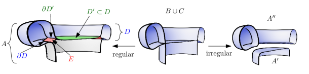
Figure 9: Non-adjacent disks, $D^{\prime}\subset D$ (or half disks $H^{\prime}\subset H$ by replacing $D$ with $H$ and $D^{\prime}$ with $H^{\prime}$). The picture is actually drawn for half disks and the disk case is obtained by doubling.

Unfortunately, the above proof contradicts minimal interior weight and does not apply when $A$ is a (non-essential) boundary parallel annulus, which may not be normal when tight. Fortunately, the half disk version contradicts tight boundary and can be applied when $A$ is essential or a boundary parallel annulus.

Lemma 7.6.

If $\sigma$ and $\tau$ both bound half disks in $A$, then they are adjacent.

Proof.

Suppose to the contrary that $\sigma$ and $\tau$ bound half disks $H$ and $H^{\prime}$ that are not adjacent across $E$. The half disks $H$ and $H^{\prime}$ are either disjoint, or, say, $H^{\prime}\subset H$.

If disjoint, then the union $H\cup E\cup H^{\prime}$ is a properly embedded disk, that after a slight isotopy, separates components of $A$, which is a contradiction.

Now suppose that $H^{\prime}\subset H$; see Figure 9. Replacing $H$ with $E\cup H^{\prime}$ is a disk swap across a ball that produces a surface $A^{\prime}$ isotopic to $A$. But notice that performing an irregular rather than regular switch at this intersection curve produces a surface with two components: one is $A^{\prime}$, and the other is an annulus $A^{\prime\prime}$ formed by identifying the ends of the rectangle $H\setminus H^{\prime}$. The irregular switch on the intersection arc yields irregular switches at the endpoints which are intersections of the boundary curves.

So while $\ell(\partial A)=\ell(\partial A^{\prime})+\ell(\partial A^{\prime\prime})$, the curve $\partial A^{\prime}\cup\partial A^{\prime\prime}$ is not normal, contains an abnormal arc by Lemma 5.5, and so there is an isotopy reducing its length. Since $\partial A^{\prime}\cup\partial A^{\prime\prime}$ is isotopic to a curve of length strictly lower than $\partial A$, each of its components has length strictly lower than $\partial A$, contradicting the minimality of the length of $\partial A$. ∎

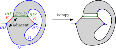
Figure 10: Adjacent disks; here $D^{\prime}\subset D$. The union $D^{\prime}\cup E\cup D$ bounds a ball after slight isotopy.

In the next two lemmas we will utilize the following observation:

Observation 7.7.

Suppose that $D$ and $D^{\prime}$ are disks that are adjacent across the exchange annulus $E$. If the disks are disjoint, then $D\cup E\cup D^{\prime}$ is, possibly after a slight isotopy, a sphere bounding a ball.

Proof.

If $D$ and $D^{\prime}$ are disjoint, we get the observation immediately, since $X$ is irreducible. If not, say if $D^{\prime}\subset D$, then fix $D$ and slightly isotope the interior of the disk $E\cup D^{\prime}$ off $D$ to the side of the exchange annulus; see Figure 10. After the isotopy $D\cup E\cup D^{\prime}$ is a sphere bounding a ball. ∎

Similarly, if $H$ and $H^{\prime}$ are half disks adjacent across the exchange rectangle $E$, then the union $H\cup E\cup H^{\prime}$ together with $\partial X$ bound a ball, possibly after a slight isotopy. Indeed, the union $H\cup E\cup H^{\prime}$ is a properly embedded disk, after first perhaps slightly isotoping, say $E\cup H^{\prime}$, when $H$ and $H^{\prime}$ are not disjoint. Its boundary $\partial H\cap\partial E\cap\partial H^{\prime}$, perhaps slightly isotoped, bounds a disk in $\partial X$ and together these disks bound a ball in $X$.

We also describe how a surface $A$ obtained as a normal sum $A=B+C$ can be obtained, under certain additional conditions, as a normal sum $A=B^{\prime}+C^{\prime}$ guided by some of the normal exchanges of $A=B+C$. Let $\mathcal{E}$ be the set of exchange bands for the normal sum $A=B+C$. Note that $|\mathcal{E}|=|B\cap C|$. We say that a subset $\mathcal{E}^{\prime}\subset\mathcal{E}$ is a consistent subset if the induced patches, components of $A\setminus\mathcal{E}^{\prime}$, can be bicolored so that two patches have different colors if they either lie on opposite sides of the same trace curve, or, are adjacent across an exchange band. (If this happens for two sides of a same patch, then in particular it cannot be bicolored.) In this case, we can see that $\mathcal{E}^{\prime}$ is the set of exchange bands for a normal sum $A=B^{\prime}+C^{\prime}$ where $B^{\prime}$ and $C^{\prime}$ are each the union of patches of a single color, connected across $\mathcal{E}^{\prime}$. See Figure 11. The same analysis holds for subsets of exchange arcs for a curve sum $\alpha=\beta+\gamma$.

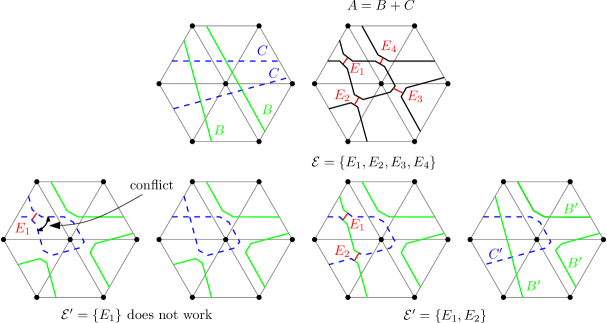
Figure 11: Summing $B$ and $C$ (upper left picture) yields $A$ (upper right picture) with the corresponding set of exchange bands/arcs $\mathcal{E}=\{E_{1},E_{2},E_{3},E_{4}\}$. Some subset $\mathcal{E}^{\prime}\subset\mathcal{E}$ may not be consistent (two lower left pictures); however, if it is consistent (two lower right pictures), then summing $B^{\prime}$ and $C^{\prime}$ yields $A$ again.

Lemma 7.8.

If $A$ is essential, then there are no disk patches. Every intersection loop is essential in $A$, $B$, and $C$.

This lemma does not apply to the boundary parallel case, because we cannot assume that disks are adjacent.

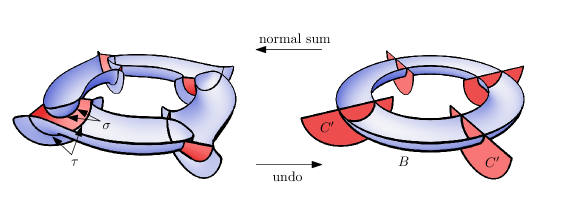
Figure 12: A cycle of adjacent half disks. Double the figure for a cycle of disks.

Proof.

This argument appears in [JO84] and [JT95]. If there is a disk patch bounded by a trace curve, then by Lemmas 7.4 and 7.5, it is adjacent across an exchange annulus $E$ to another disk. The adjacent disk is not a single patch,since if it were, $\mathcal{E}\setminus E$ would be a consistent subset, and we could expresses $A$ as a sum $A=B^{\prime}+C^{\prime}$, where $B^{\prime}$ and $C^{\prime}$ are isotopic to $B$ and $C$, respectively, but $|B^{\prime}\cap C^{\prime}|<|B\cap C|$, a contradiction. Thus, the adjacent disk contains trace loops. Pass to an innermost trace loop bounding a disk patch and repeat.

This process can be continued arbitrarily, and therefore must eventually repeat. Thus there is a shortest cycle of adjacent disks, each biting the tail patch of its predecessor across some exchange annulus; see Figure 12. Note that the cycle has length 1 when $D^{\prime}\subset D$ for some pair of adjacent disks $D$ and $D^{\prime}$. By irreducibility, the union of a pair of adjacent disks and their exchange annulus is a sphere bounding a ball, and the union of these balls is a solid torus.

Let $\mathcal{E}^{\prime}$ be the subset of $\mathcal{E}$ along which the cycle of disks is adjacent. Then $\mathcal{E}^{\prime}$ is seen to be a consistent subset of $\mathcal{E}$ by coloring all annulus patches on the boundary of the solid torus with one color, and all other patches with the other. This expresses $A$ as the sum of surfaces $A=B^{\prime}+C^{\prime}$ where $B^{\prime}$ is a normal torus bounding a solid torus.

Adding $B^{\prime}$ to $C^{\prime}$ corresponds to a fractional Dehn twist in $B^{\prime}$. Since $B^{\prime}$ bounds a solid torus, there is an isotopy of the solid torus that undoes the twist and carries $C^{\prime}$ to $A$. So $C^{\prime}$ is isotopic to $A$ but with strictly lower complexity $\operatorname{cpx}(C^{\prime})=\operatorname{cpx}(A)-\operatorname{cpx}(B^{\prime})$—a contradiction. ∎

We repeat the above argument to work in the context of trace arcs and half disks. This argument does apply to boundary parallel annuli, as their half disks are known to be adjacent. The proof will reach a contradiction to the tightness of $\partial A$.

Lemma 7.9.

No trace arc bounds a half disk in $A$.

Proof.

When $A$ is a boundary parallel annulus, Lemma 7.8 does not apply, and trivial trace loops may be present. So we will refer to outermost (in $A$) half disks instead of half disk patches. An outermost half disk in $A$ does not contain trace arcs, but, is not a patch if it contains trace loops. If there is an outermost half disk $H$ bounded by a trace arc, then by Lemmas 7.4 and 7.6, it is adjacent across an exchange rectangle $E$ to another half disk $H^{\prime}$.

The adjacent half disk $H^{\prime}$ is not outermost: If $H$ and $H^{\prime}$ are both outermost, then $H\cup E\cup H^{\prime}$ is a properly embedded disk that meets $\partial X$ in a disk bounding the curve $h\cup e\cup h^{\prime}\cup e^{\prime}$, where $h=H\cap\partial X$, $h^{\prime}=H^{\prime}\cap\partial X$ and $e$ and $e^{\prime}$ are exchange arcs, the two components of $E\cap\partial X$. Since $h$ and $h^{\prime}$ are sub-arcs of $\partial B$ and $\partial C$, we can see, by undoing the exchanges $e$ and $e^{\prime}$, that $\partial B$ and $\partial C$ bound a bigon and are thus not snug, a contradiction.

Thus, the adjacent half disk is not outermost and contains at least one trace arc. Pass to an innermost trace loop bounding a outermost half disk and repeat. This process can be continued arbitrarily, and therefore must eventually repeat. Thus, there is a shortest cycle of adjacent half disks, each biting the tail patch of its predecessor across some exchange rectangle; see Figure 12. Note that the cycle has length 1 when $H^{\prime}\subset H$ for some pair of adjacent half disks $H$ and $H^{\prime}$. By irreducibility and incompressibility of $\partial X$, the union of a pair of adjacent half disks and their exchange rectangle is a disk that co-bounds a ball with a disk in $\partial X$, and the union of all these balls is a solid torus meeting $\partial X$ in an annulus.

Let $\mathcal{E}^{\prime}$ be the subset of $\mathcal{E}$ along which the cycle of half disks is adjacent. Then $\mathcal{E}^{\prime}$ is seen to be a consistent subset of $\mathcal{E}$ by coloring all rectangle patches on the boundary of the solid torus with one color, and all other patches with the other. This expresses $A$ as the sum of surfaces $A=B^{\prime}+C^{\prime}$ where $B^{\prime}$ is a normal boundary parallel annulus.

Adding $B^{\prime}$ to $C^{\prime}$ corresponds to a fractional Dehn twist in $B^{\prime}$. Since $B^{\prime}$ is boundary parallel, there is an isotopy of the solid torus that undoes the twist and carries $C^{\prime}$ to $A$. So $C^{\prime}$ is isotopic to $A$ but with shorter length $\ell(C^{\prime})=\ell(A)-\ell(B^{\prime})$, a contradiction. ∎

We know that $A$ is incompressible, and thus by Proposition 4.2 it is either an essential annulus or Möbius band, or a boundary parallel annulus. We deduce that in both cases it means that $B$ is essential.

Lemma 7.10.

If $A$ is a boundary parallel annulus, then $B$ is essential (not a boundary parallel annulus).

Proof.

Suppose that $B$ is a boundary parallel annulus. If $\partial C=\emptyset$ then $\partial B=\partial A$, and hence $A$ and $B$ are isotopic, contradicting the fact that $A$ was chosen to have least complexity.

So we have $A=B+C$, where all three have non-empty tight boundary and $A$ and $B$ are both boundary parallel annuli. Then $\partial A=2a$ and $\partial B=2b$, where $a$ and $b$ are tight essential curves since $A$ and $B$ have tight boundaries. Since all normal coordinates of $\partial A$ and $\partial B$ are even, it follows that $\partial C=2c$ for some tight essential curve $c$ by Lemma 6.8.

Each pair, $2b$ and $2c$, of parallel curves bounds an annulus in $\partial X$. Normally isotope $B$ and $C$ so that these annuli are very thin and intersect in a collection of squares, each contained in a face of $\partial X$. Pick a particular square. Each of its corners is an endpoint of an intersection arc between $B$ and $C$. All corners have the same normal sign. It follows that the exchange rectangles for corners on the same edge lie on opposite sides of $A$; see Figure 13.

Thus, there is an exchange rectangle $R$ properly embedded inside the solid torus $T$ that is bounded by $A$ and $A_{\partial X}\subset\partial X$, the annulus into which $A$ is isotopic. Then $\partial R$ is a compressing disk for $T$ since it meets $A$ in a pair of arcs that are essential by Lemma 7.9 and meets $A_{\partial X}$ in a pair of arcs that are essential by Lemma 6.5. But this contradicts the fact that $A$ is boundary parallel to $A_{\partial X}$. The unique, up to isotopy, compressing disk for $T$ meets $A$ and $A_{\partial X}$ each in a single essential arc. ∎

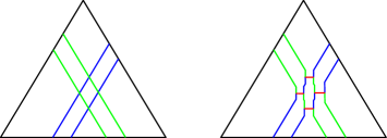
Figure 13: Annuli between $2b$ and $2c$ intersecting in a square. After regular exchanges there are four exchange arcs in which exchange rectangles start. At least one of these rectangles (actually two) have to be inside $T$.

Lemma 7.11.

If $A$ is essential then $B$ is essential (not a boundary parallel annulus).

Proof.

We first note, as in [JT95], that each disk patch is incompressible and boundary incompressible. Any (boundary) compressing disk for a patch has its boundary in the essential surface $A$ and therefore meets it in a trivial curve. This, in turn, implies the existence of a (half) disk patch.

In contradiction, suppose $B$ is a boundary parallel annulus. By Lemma 7.8, $B$ and $C$ intersect in curves that are essential in both. These curves are either core loops or spanning arcs for $B$.

But they cannot be spanning arcs: If so, then there is a boundary compressing disk $D$ for $B$ so that $\partial D\cap B\cap\partial C=\emptyset$. Choose $D$ to be such a boundary compressing disk that meets $C$ in the minimal number of curves. Let $D^{\prime}$ be a disk bounded by an innermost loop, outermost arc, or when $C\cap D=\emptyset$, let $D=D^{\prime}$. By minimality $D^{\prime}$ meets a patch in an essential curve and is thus a (boundary) compressing disk for a patch. This contradicts Observation 7.7.

We proceed assuming that $B\cap C$ is a collection of loops essential in both $B$ and $C$. Then the patches of $B$ and $C$ are annuli because each component of $C$ has zero Euler characteristic. As before, choose a boundary compressing disk $D$ for $B$ that meets $C$ in the minimal number of curves.

By minimality of $D$ and essentiality of patches, no curve of intersection is a closed loop or an arc with endpoints both in $\partial X$. It follows that $\gamma$, an outermost arc of intersection, co-bounds a bigon or half bigon $D^{\prime}$, with an arc $\beta\subset B\cap\partial D$. (Figure 3, with different labelling). By minimality of $|D\cap C|$, $\beta$ is a spanning (essential) arc for an annulus patch $A_{B}\subset B$ and $\gamma$ is a spanning arc for a patch $A_{C}\subset C$. The patches meet in either one (half bigon) or two (bigon) intersection loops. Moreover, because $X$ is irreducible and has incompressible boundary, $A_{B}$ and $A_{C}$ are parallel across the solid torus that they bound. Thus, Figure 3 is a cross-section of the total intersection, $\textit{(half)bigon}\times S^{1}$.

What does the normal addition $A=B+C$ do with the patches $A_{B}$ and $A_{C}$? It cannot trade them as in the figure, because then, performing only the trade and no other exchanges produces normal surfaces $B^{\prime}$ and $C^{\prime}$ isotopic to $B$ and $C$ but with fewer intersections, contradicting our assumption that we had minimized $|B\cap C|$. Nor, in the half bigon case, can it attach $A_{B}$ and $A_{C}$. For this means $A$ has a boundary parallel annulus component. This rules out the half bigon case. And, in the bigon case, it cannot attach $A_{B}$ to $A_{C}$ along both curves, for if it did, a component of $A$ would be a torus bounding a solid torus. So $A_{B}$ and $A_{C}$ are attached along one intersection loop, but not along the other. But then $A_{B}\cup A_{C}$ is parallel to the zero weight exchange annulus for the intersection loop where they were not attached.

Form a Haken sum $A^{\prime}$ by performing all regular exchanges, except perform an irregular exchange (fold) along the curve corresponding to the zero weight annulus. This is similar to the situation in Figure 9, although the context is a bit different. Then one component of $A^{\prime}$ is isotopic to $A$ and the other, call it $A^{\prime\prime}$, is a torus bounding a solid torus. But $A^{\prime}\cup A^{\prime\prime}$ is not normal because of the irregular switch. As in the end of the proof of Lemma 7.5, we conclude that $A^{\prime}\cup A^{\prime\prime}$ is either boundary compressible, not least length, or, $A$ is not tight. All are contradictions. ∎

This completes the proof of Proposition 7.2.

8 Constructing an annulus curve $\alpha$

As usual, we assume that $X$ is irreducible, orientable with incompressible boundary and presented via a 0-efficient triangulation.

Definition 8.1.

An annulus curve $\alpha$ is a properly embedded (multicomponent) normal curve in $\partial X$ with the following property: There exists a collection $\mathcal{A}$ of pairwise disjoint properly embedded essential annuli in $X$ such that $\alpha\subseteq\partial\mathcal{A}$ and $\alpha$ represents all normal isotopy classes of boundary components of $\mathcal{A}$ exactly once, i.e., for every annulus $A\in\mathcal{A}$ and every component $\gamma$ of $\partial A$, there is exactly one component of $\alpha$ that is normally isotopic to $\gamma$.

The following proposition provides an annulus curve that can be used to track essential annuli. Each boundary curve of a tight essential annulus either appears in the curve or meets the curve.

Proposition 8.2.

Let $X$ be an irreducible, orientable manifold with incompressible boundary presented via a 0-efficient triangulation with $t$ tetrahedra. Then there is a tight normal annulus curve $\alpha$ so that:

1. $\alpha$ is maximal, by which we mean that if $A\subset X$ is an essential annulus or Möbius band whose boundary is tight and disjoint from $\alpha$, then each boundary component of $\partial A$ is normally isotopic to a component of $\alpha$.

2. $|\alpha|$, the number of components of $\alpha$, is smaller than $4t$.

3. $\ell(\alpha)$ is bounded by a computable function of $t$.

The bound for $\ell(\alpha)$ we obtain from our proof is an $O(t)$-times iterated exponential, and this is currently a bottleneck of the whole algorithm.

The proposition follows in a simple way from the next two lemmas.

Lemma 8.3.

Suppose $\alpha_{0}$ is a tight, normal annulus curve in the boundary of an irreducible, orientable manifold with incompressible boundary and a 0-efficient triangulation. Let $A$ be an essential annulus with tight boundary that is disjoint from $\alpha_{0}$, and such that a component of $\partial A$ is not normally isotopic into $\alpha_{0}$.

Then there is a tight normal annulus curve $\alpha$ such that $\alpha_{0}\subsetneq\alpha$ and $\ell(\alpha)$ is bounded by a computable function of $t$ and $\ell(\alpha_{0})$.

Proof.

The curve $\alpha_{0}$ can be regarded as a fence in the marked triangulation $(\mathcal{T},\alpha_{0}\cap\mathcal{T}^{1})$. The annulus $A$ has tight boundary disjoint from the fence $\alpha_{0}$. By isotoping the interior of $A$ (if necessary) while keeping its boundary $\partial A$ fixed, we may assume that $A$ is tight and hence, by Proposition 7.1, normal.

Write $A=F_{1}+F_{2}+\cdots+F_{k}$, a sum of connected fundamentals for the marked triangulation $(\mathcal{T},\alpha_{0}\cap\mathcal{T}^{1})$. By Lemma 6.8 and by Proposition 6.10, respectively, each boundary $\partial F_{i}$ is tight and disjoint from the fence $\alpha_{0}$. Since $\ell(\partial F_{i})\leq|F\cap\mathcal{T}^{1}|$, by Proposition 5.2, $\ell(\partial F_{i})$ is bounded by a computable function of $t$ and $\ell(\alpha_{0})$, the number of marking points. By Proposition 7.2, each $F_{i}$ with non-empty boundary is an essential annulus or Möbius band.

Moreover, there must be a summand with a boundary component that is not normally isotopic into $\alpha_{0}$. Otherwise, each component of the boundary sum $\partial A=\partial F_{1}+\partial F_{2}+\cdots+\partial F_{k}$, would be normally isotopic to a component of the fence $\alpha_{0}$. This would imply that the summands are pairwise disjoint after a normal isotopy and, that each component of $\partial A$ is itself normally parallel to a component of the fence $\alpha_{0}$, contradicting our assumption.

Fix such a summand with a boundary component $\alpha^{\prime}$ not normally isotopic into $\alpha_{0}$. We will construct a new annulus curve $\alpha$ that contains both $\alpha_{0}$ and $\alpha^{\prime}$ (which ensures $\alpha_{0}\subsetneq\alpha$).

Let $A^{\prime}$ be the summand if it is an essential annulus or twice the summand if it is a Möbius band.

Let $\mathcal{A}_{0}$ be a collection of pairwise disjoint essential annuli witnessing that $\alpha_{0}$ is an annulus curve, i.e., $\alpha_{0}\subseteq\partial\mathcal{A}_{0}$ and $\alpha_{0}$ represents all normal isotopy classes of boundary components of $\mathcal{A}_{0}$ exactly once. By construction of the annulus $A^{\prime}$, its boundary $\partial A^{\prime}$ is disjoint from the fence $\alpha_{0}$ and hence from $\partial\mathcal{A}_{0}$, and one boundary component of $A^{\prime}$ is the curve $\alpha^{\prime}$.

We isotope $A^{\prime}$, leaving the boundary fixed, to minimize components of intersection $|A^{\prime}\cap\mathcal{A}_{0}|$, and we distinguish two cases.

The first case is that $A^{\prime}$ misses $\mathcal{A}_{0}$. Then $\mathcal{A}=\mathcal{A}_{0}\cup A^{\prime}$ is a collection of pairwise disjoint properly embedded essential annuli. We define $\alpha$ to be the annulus curve corresponding to $\mathcal{A}$. More precisely, $\alpha^{\prime}$ is one of the boundary components of $A^{\prime}$. If the other boundary component is normally isotopic to $\alpha^{\prime}$ or to some component of $\alpha_{0}$, we set $\alpha=\alpha_{0}\cup\alpha^{\prime}$, and otherwise, we set $\alpha=\alpha_{0}\cup\partial A^{\prime}$. Thus, $\alpha$ is an annulus curve, as witnessed by $\mathcal{A}$, $\alpha_{0}\subsetneq\alpha$, and $\ell(\alpha)$ is bounded by a computable function of $t$ and $\ell(\alpha_{0})$ since $\ell(\partial A^{\prime})$ is.

The second case is that $A^{\prime}$ intersects $\mathcal{A}_{0}$. In this case, since $\partial A$ and $\partial\mathcal{A}_{0}$ are disjoint, a standard innermost loop argument shows that all curves of intersection are essential, i.e., core curves in the annuli; see the proof of Lemma 4.3.

If $A^{\prime}$ meets $\mathcal{A}_{0}$, let $\alpha^{\prime\prime}\subset A^{\prime}$ be the core intersection curve closest to $\alpha^{\prime}$, and let $\tilde{A}$ be the corresponding annulus in $\mathcal{A}_{0}$. Then $\alpha^{\prime}$ and $\alpha^{\prime\prime}$ co-bound a sub-annulus $A^{\prime\prime}\subset A^{\prime}$ whose interior misses $\partial\mathcal{A}_{0}$.

Note that $\alpha^{\prime\prime}$ splits the annulus component $\tilde{A}$ of $\mathcal{A}_{0}$ into annuli $A_{1}$ and $A_{2}$. Then $\alpha^{\prime}$ is a boundary curve of both of the annuli $A^{\prime\prime}\cup A_{1}$ and $A^{\prime\prime}\cup A_{2}$, both of these are disjoint from $\mathcal{A}_{0}$, and at least one of them is essential.

Suppose w.l.o.g. that $A^{\prime\prime\prime}=A^{\prime\prime}\cup A_{1}$ is essential. Then $\mathcal{A}=\mathcal{A}_{0}\cup A^{\prime\prime\prime}$ is a collection of pairwise disjoint essential annuli witnessing that $\alpha:=\alpha_{0}\cup\alpha^{\prime}$ is an annulus curve (since one boundary component of $A^{\prime\prime\prime}$ is $\alpha^{\prime}$ and the other one is a boundary component of $\tilde{A}\in\mathcal{A}_{0}$ and hence already represented in $\alpha_{0}$). Moreover, as in the first case, $\ell(\alpha)$ is bounded by a computable function of $t$ and $\ell(\alpha_{0})$ since $\ell(\partial A^{\prime})$ and hence $\ell(\alpha^{\prime})$ is. ∎

Lemma 8.4.

Let $\alpha$ be an essential curve embedded in a a connected closed orientable triangulated surface $F$ with $f$ faces, such that no pair of components of $\alpha$ are isotopic. Then $|\alpha|<f$.

Proof.

The result holds trivially for a torus, which requires at least two faces to triangulate and allows $\alpha$ to have at most one component.

Now suppose that the genus of the surface is $g\geq 2$. We claim that then $\alpha$ has at most $3g-3$ components. We may assume that $\alpha$ is a maximal collection of non-parallel curves, and hence it decomposes $F$ into $p$ pairs of pants (spheres with 3 holes) [FM11, Sec. 8.3.1]. Each pair of pants has Euler characteristic $-1$, and because the Euler characteristic of the boundary of a pair of pants is zero, the Euler characteristic of the surface is additive over the pants, $\chi(F)=-p=2-2g$. Because each curve is on the boundary of two pairs of pants, we have $|\alpha|=\frac{3}{2}p=3g-3$.

We have $\chi(F)=2-2g=f-e+v$, where $e=\frac{3}{2}f$ is the number of edges and $v$ is the number of vertices. Then $g=\frac{f}{4}+1-v\leq\frac{f}{4}$ and $|\alpha|\leq 3g-3\leq\frac{3}{4}f<f$, as desired. ∎

We now complete the proof of the main proposition.

Proof of Proposition 8.2.

The annulus curve $\alpha$ can be constructed iteratively, starting with $\alpha=\emptyset$. If, at any stage, the maximality property (1) is not satisfied, we apply Lemma 8.3 to add a distinct component to $\alpha$.

We claim that the process terminates after adding at most $4t$ components: By Lemma 8.4, each boundary component of $X$ contains fewer components of $\alpha$ than it has faces (here, we are using that $\alpha$ is tight, so by Lemma 6.3, the fact that no two components of $\alpha$ are normally isotopic also implies that no two of them are isotopic). Thus, in total, $\alpha$ has fewer components than $X$ has boundary faces and the number of boundary faces is bounded by $4t$. This is (2).

By Lemma 8.3, the first component added has length bounded by a computable function of $t$. Every subsequent component added has length bounded by a computable function of $t$ and the total length of the preceding components. Since the number of components is less than $4t$, the total length of the curve is bounded by a computable function of $t$. ∎

9 Curves bounding boundary parallel annuli

In the previous section we constructed the annulus curve $\alpha$, which will be used to bound the coefficients of essential annulus summands in the planar (almost) meridional surface $P$. In this section we construct $\Gamma$, a collection of curves bounding normal boundary parallel annuli. Later, the curves of $\Gamma$ will act as fences, and will be used to rule out boundary parallel annulus summands altogether.

Proposition 9.1.

Suppose $X$ is an irreducible, orientable manifold with incompressible boundary and presented via a 0-efficient triangulation with $t$ tetrahedra. Let $\alpha$ be the tight normal annulus curve given by Proposition 8.2. Then there is a finite set $\Gamma$ of tight essential curves, possibly mutually intersecting, such that:

1. If $B$ is a normal boundary parallel annulus with tight boundary that is disjoint from $\alpha$, then each boundary component of $B$ is normally isotopic either to a component of $\alpha$ or to a curve of $\Gamma$.

2. $|\Gamma|$ and $\max_{\gamma\in\Gamma}\ell(\gamma)$ are bounded by a computable function of $t$.

Proof.

Let $\alpha$ be given by Proposition 8.2. Then $\alpha$ is a fence in the marked triangulation $(\mathcal{T},\alpha\cap\mathcal{T}^{1})$. Let $\Gamma$ be the set of the boundaries of all boundary parallel annuli that are fundamental in the marked triangulation $(\mathcal{T},\alpha\cap\mathcal{T}^{1})$ and disjoint from the fence $\alpha$. Then (2) follows from Proposition 5.2.

Now we want to verify (1). Let $B$ be a normal boundary parallel annulus with tight boundary disjoint from the fence $\alpha$. By isotoping $B$ we can assume that $B$ is least complexity.

If $B$ is a fundamental, then its boundary has already been included in $\Gamma$ and we are done. If not, then $B$ can be written as a sum of fundamentals for $(\mathcal{T},\alpha\cap\mathcal{T}^{1})$, $B=F_{1}+F_{2}+\cdots+F_{k}$. By Proposition 7.2, each $F_{i}$ with boundary is an essential annulus or Möbius band. Since $B$ is disjoint from the fence $\alpha$, each $F_{i}$ has boundary disjoint from $\alpha$. Hence, by Proposition 8.2, each $F_{i}$ has boundary components normally isotopic to $\alpha$. But as observed in the proof of Proposition 8.2, this implies that each boundary component of $B$ is normally isotopic to $\alpha$, as required. ∎

10 Planar meridional surfaces

In this section we consider a planar (almost) meridional surface $P$ in $X$ and a collection $\mathcal{A}$ of disjoint essential annuli. The collection $\partial\mathcal{A}$ of the boundaries of the annuli in $\mathcal{A}$ forms a collection of disjoint curves (loops) in $\partial X$, and $\partial P$ is another collection of disjoint loops.

We want to move $P$ by means of a self-homeomorphism $h\colon X\to X$ in such a way that the number of intersections of these two collections, $\partial\mathcal{A}$ and $\partial P$, becomes bounded; more precisely, we need a bound of the form $C(t)|\mathcal{A}|\cdot|\partial P|$. This is formulated in Proposition 10.3 below; the self-homeomorphism $h$ is going to be one of two ways of changing the original embedding of $X$ in $S^{3}$ in order to get a short meridian.

First we collect auxiliary results. We begin with a corollary of the main result of [MSTW13], which was developed for the purpose of proving a result in the spirit of Proposition 10.3.

Lemma 10.1 ([MSTW13, Cor. 1.6]).

Let $S$ be connected surface, i.e., a connected compact $2$-manifold with boundary, of genus $g$. Let $(\alpha_{1},\ldots,\alpha_{m})$ be a system of disjoint curves (properly embedded arcs and loops) in $S$, and let $(\beta_{1},\ldots,\beta_{n})$ be another such system. Then there is a homeomorphism $\varphi\colon S\to S$ fixing $\partial S$ pointwise such that the total number of intersections of $\alpha_{1},\ldots,\alpha_{m}$ with $\varphi(\beta_{1}),\ldots,\varphi(\beta_{n})$ is at most $K(g)mn$, where $K(g)$ is a computable function depending only on $g$ (in fact, $K(g)=O(g^{4})$).

We remark that for our further approach a bound of the form $K(g,m)n$ would also be sufficient. Such a bound, even independent of $g$, was obtained independently by Geelen, Huynh, and Richter [GHR13], but only under the additional assumption that the union of the $\beta_{i}$ does not separate $S$. Thus, we cannot directly use their result here; the extra assumption could probably removed, but it is easier to use the bounds from [MSTW13].

We also need the following, probably standard, lemma.

Lemma 10.2.

Let $G=(V,E)$ be a graph with $n>2$ vertices embedded in $S^{2}$, possibly with loops and multiple edges. Let us assume that no two parallel edges (connecting the same two vertices) and no two parallel loops (attached to the same vertex) are isotopic by an isotopy fixing the end-vertices and avoiding the other vertices. We also assume that there is no contractible loop $\ell$; that is, both the interior and exterior of each loop contain a vertex. Then $|E|\leq 3n-6$.

Proof.

If $G$ contains neither loops nor multiple edges, then this is just the usual bound for the number of edges of a simple planar graph. It remains to resolve loops and multiple edges.

First let $\ell$ be a loop with an endpoint $v$. It splits $S^{2}$ into two regions $X$ and $Y$. Let $F_{X}$ resp. $F_{Y}$ be the face of $G$ inside $X$ resp. $Y$ bounded by $\ell$. Then $F_{X}$ has to contain a vertex $v_{X}\neq v$, for otherwise, $\ell$ can be contracted to $v$ or it is isotopic to another loop with endpoint $v$.

Similarly, we have a vertex $v_{Y}$ in $F_{Y}$. Note that $v_{X}$ and $v_{Y}$ are not connected with an edge. We can remove $\ell$ from the graph and connect $v_{X}$ and $v_{Y}$ with an edge, keeping the graph embedded in $S^{2}$ and satisfying the isotopy assumptions. This way we can remove all loops without increasing the number of edges; see Figure 14.

Similarly, if we have two parallel edges, we can remove one of them and add a new edge as compensation, reducing the number of pairs of parallel edges. In this way, we get a simple planar graph and the desired bound. ∎

Figure 14: Removing loops and parallel edges.

Proposition 10.3.

Let $X$ be an orientable, irreducible manifold with incompressible boundary. Let $P\subset X$ be a properly embedded planar surface that is either essential, or strongly irreducible and boundary strongly irreducible. Let $\mathcal{A}\subset X$ be a collection of pairwise disjoint essential annuli. Then there is a homeomorphism $h\colon X\to X$ so that $|\partial h(P)\cap\partial\mathcal{A}|<C|\mathcal{A}|\cdot|\partial P|$, where $C=C(t)$ is a computable function of the number $t$ of tetrahedra in the triangulation of $X$.

Proof.

Using either Lemma 4.3 or Lemma 4.7, we may isotope $P$ so that its intersection with $\mathcal{A}$ is essential, that is every component of $P\cap\mathcal{A}$ is a curve that is essential in both $P$ and $A$. This implies that the result holds when $P$ is a disk, for then $P$ contains no essential curves, and thus $P\cap\mathcal{A}$ is empty. We proceed assuming $|\partial P|>1$.

In $\mathcal{A}$ every intersection arc is a spanning arc and every intersection loop is the core curve of an annulus. This is illustrated below in the left picture, while the right picture shows the intersection curves in $P$:

Say that two arcs belong to the same parallel class if they are isotopic in $P$. If $|\partial P|=2$, then $P$ is an annulus and there is at most one parallel class of intersection arcs. When $|\partial P|>2$, form a planar graph by treating each boundary component as a vertex and each parallel class of arcs as an edge. The number of edges, hence parallel classes, is bounded by $3(|\partial P|-2)$ by Lemma 10.2. We can cover the cases when $P$ is an annulus or disk by reducing this last bound slightly. In all cases the number of parallel classes of arcs is bounded by $3(|\partial P|-1)<3|\partial P|$.

A band in $X$ is an embedded, but not properly embedded, rectangle meeting $\partial X$ in precisely its top and bottom sides. For each parallel class of intersection arcs in $P$, we may choose a band $B_{j}$ that is a sub-surface of $P$, contains all intersection arcs in the class, and meets no other curves of intersection. Then $\mathcal{B}$, the union of all such bands, has at most $3|\partial P|$ components and contains all arcs, but no loops, of the intersection $P\cap\mathcal{A}$.

Next, let us draw the core curve $\alpha_{i}$ for every annulus in $A_{i}\in\mathcal{A}$, and a curve $\beta_{i}$ parallel to the top and bottom sides (those in $\partial X$) in the middle of each band $B_{j}$. Let us think of these $\alpha_{i}$ and $\beta_{j}$ as being (locally) horizontal and lying in the same level; then, again locally, $A_{i}$ is a vertical “wall” through $\alpha_{i}$ and $B_{j}$ is a vertical “wall” through $\beta_{j}$. We have the $A_{i}$ and $B_{j}$ fibered with segments, as in the left picture, and so the union $\mathcal{A}\cup\mathcal{B}$ has the structure of an $I$-bundle $M_{0}$ over $(\bigcup_{i}\alpha_{i})\cup(\bigcup\beta_{j})$, where $I$ is the interval $[-1,1]$; see the left picture below:

As the picture illustrates, some of the $A_{i}$ or $B_{j}$ may be twisted between the intersections with the others.

Next the $I$-bundle structure on $\mathcal{A}\cup\mathcal{B}$ can be extended to a sufficiently small regular neighborhood $N(\mathcal{A}\cup\mathcal{B})$. Indeed, we can consider the regular neighborhood as the star of $\mathcal{A}\cup\mathcal{B}$ (say in the second barycentric subdivision of some triangulation); see [RS72, Chapter 3]. Therefore, $N(\mathcal{A}\cup\mathcal{B})$ has locally structure as product of $\mathcal{A}\cup\mathcal{B}$ with $I$.

We obtain an $I$-bundle $M$ over a base surface $S$ forming a narrow ribbon along the $\alpha_{i}$ and the $\beta_{j}$. This is illustrated locally in the right picture above.

The plan is now to use Lemma 10.1 (untangling curves in a surface) for the systems of curves $\alpha_{i}$ and $\beta_{j}$ within $S$, which yields a self-homeomorphism $\varphi\colon S\to S$ fixing $\partial S$ pointwise, such that the number of intersections of the $\alpha_{i}$ with the $\varphi(\beta_{j})$ is suitably bounded. Then we want to extend $\varphi$ to a bundle self-homeomorphism $h\colon M\to M$ that is the identity over $\partial S$ (i.e., on the vertical walls bounding $M$ in the picture). After that, $h$ can be extended identically to $X\setminus M$ and we will be done.

There are two issues to be handled. First, in order to use Lemma 10.1, bound the genus of each component of $S$ by a computable function of $t$; we will actually obtain an $O(t)$ bound.

To this end, we observe that $S$ is double-covered by a surface $\tilde{S}:=N(\mathcal{A}\cup\mathcal{B})\cap\partial X$. Let $K$ be a component of $S$ and $\tilde{K}$ be the corresponding double cover of $K$ in $\tilde{S}$. In particular, $\chi(\tilde{K})=2\chi(K)$. For a surface $F$, we let $b(F)$ denote the number of boundary components, and define $g_{e}(F):=2-\chi(F)-b(F)$. If $F$ is connected, this value is known as the Euler genus of $F$. Then we get

$$g_{e}(K)=1+g_{e}(\tilde{K})/2-b(K)+b(\tilde{K})/2\leq 1+g_{e}(\tilde{K})/2.$$

Let $\tilde{Q}$ be a component of $\tilde{K}$ ($\tilde{K}$ has two components if $K$ is orientable). Since $\tilde{Q}\subseteq\partial X$, we have $g_{e}(\tilde{Q})\leq g_{e}(X^{\partial}_{Q})$ where $X^{\partial}_{Q}$ is the component of $\partial X$ containing $\tilde{Q}$. The Euler genus of $X^{\partial}_{Q}$ is bounded by $O(t)$, since $\partial X^{\partial}_{Q}=\emptyset$ and $|\chi(X^{\partial}_{Q})|=O(t)$ (note that the number of triangles, edges and vertices in triangulation of $X$ are all bounded by $O(t)$).

Altogether $g_{e}(\tilde{Q})=O(t)$, and since $\tilde{K}$ has at most two components, $g_{e}(K)=O(t)$. Since the genus of a surface is at most twice the Euler genus, we also obtain $g(K)=O(t)$.

By applying Lemma 10.1 as announced above, working in each component $K$ of $S$ separately and then summing up, we obtain a self-homeomorphism $\varphi$ of $S$, fixed pointwise on $\partial S$, such that the total number of intersections of the $\alpha_{i}$ with the $\varphi(\beta_{j})$ is at most $C_{0}(t)|\mathcal{A}|\cdot|\mathcal{B}|\leq 3C_{0}(t)|\mathcal{A}|\cdot|\partial P|$, where $C_{0}(t)$ is a computable function of $t$.

It remains to deal with the second and last issue, namely, showing that $\varphi$ extends to a bundle self-homeomorphism $h\colon M\to M$ that is identical over $\partial S$. Here we may assume w.l.o.g. that $S$, and hence $M$, are connected.

By the assumption, $M$ is embedded in $X$, and so it is orientable. It follows that if the surface $S$ is orientable, then $M$ is actually the product $S\times[-1,1]$, and the extension of $\varphi$ to $h$ is obvious.

So let $S$ be non-orientable; then $M$ is non-trivially twisted and there are no global coordinates. For a subset $S^{\prime}$ of $S$ we will use a notation $S^{\prime}\widetilde{\times}I$ for the subbundle of $M$ consisting of points of $M$ that project to $S^{\prime}$. (In particular, we also regard $M$ as $S\widetilde{\times}I$.)

For any connected non-orientable surface $S$ there is a non-separating arc $\sigma\subset S$ with both endpoints on the same boundary component for which $S_{\sigma}$, which is $S$ cut along $\sigma$, is an orientable surface. We also let $f_{\sigma}\colon S_{\sigma}\to S$ be the map gluing $S_{\sigma}$ back to $S$.

Thus, after cutting $M$ along $\sigma\times I$, we obtain a product bundle $M_{\sigma}$, homeomorphic to $S_{\sigma}\times I$. In the boundary of $M_{\sigma}$ we see two rectangle scars from cutting along $\sigma\times I$. We get the twisted bundle $M$ back by gluing $M_{\sigma}$ to itself along the rectangles so that the top of one is glued to the bottom of the other.

Now the given homeomorphism $\varphi\colon S\to S$ also takes $\sigma$ to a curve $\varphi(\sigma)$ that has the same separation properties. We define $S_{\varphi(\sigma)}$ and $f_{\varphi(\sigma)}$ in the same way as $S_{\sigma}$ and $f_{\sigma}$ above. The homeomorphism $\varphi$ also induces a homeomorphism $\varphi^{\prime}\colon S_{\sigma}\to S_{\varphi(\sigma)}$ satisfying $f_{\varphi(\sigma)}\circ\varphi^{\prime}=\varphi\circ f_{\sigma}$.

The homeomorphism $\varphi^{\prime}$ can be extended to a homeomorphism of the product bundles $h^{\prime}\colon S_{\sigma}\times I\to S_{\varphi(\sigma)}\times I$ in two ways (by either keeping $I$ or swapping it). By gluing back along the rectangular scars, $h^{\prime}$ induces a homeomorphism $h\colon M\to M$.

Recall that $M$ is orientable since it embeds into $X$. Since we had two choices for $h^{\prime}$ we select one for which $h$ is an orientation preserving automorphism. It follows that whenever $K$ is a boundary component of $S$, then $h$ is the identity on $K\widetilde{\times}I$ (it cannot flip $I$ here since such a flip would reverse the orientation on $\partial M$, hence on $M$). ∎

11 Proof of the short-meridian theorem

We already have almost all of the ingredients ready to prove Theorem 1.4, following the outline from Section 2.

We assume that $X$ is irreducible, has incompressible boundary (which we may assume to be nonempty), embeds in $S^{3}$, and has a 0-efficient triangulation with $t$ tetrahedra. Note that the second conclusion of the following lemma may require a re-embedding of $X$ into $S^{3}$.

Lemma 11.1.

$X$ contains a planar surface $P$ so that:

1. $P$ is essential, or, strongly irreducible and boundary strongly irreducible, and

2. $\partial P$ is meridional or almost meridional in some embedding of $X$ in $S^{3}$.

Proof.

Since $X$ embeds in $S^{3}$, we can apply the result of Fox [Fox48] that shows $X$ may be embedded so that $S^{3}\setminus interior(X)$ is a collection of handlebodies.

Then we may view $X$ as the exterior, $X=S^{3}\setminus N(\Gamma)$, where $\Gamma$ is a graph consisting of a spine of each handlebody. In this context, we may apply Theorem 3 of Li [Li10] that states that $X$ contains a planar surface that is either: (1) meridional, strongly irreducible, and boundary strongly irreducible, or (2) almost meridional and essential , or (3) non-separating, almost meridional, and incompressible. By Lemma 4.5, case (3) reduces to case (2), and the lemma follows. ∎

Lemma 11.2.

Let $P$ be a surface satisfying the conditions of Lemma 11.1, and let $h\colon X\to X$ be a homeomorphism. Then $h(P)$ satisfies the conditions of Lemma 11.1 for some re-embedding of $X$.

Proof.

Because the homeomorphism $h$ maps any disk in $X$ to a disk in $X$, $P$ is essential if and only if $h(P)$ is essential; and, $P$ is strongly irreducible and boundary strongly irreducible if and only if $h(P)$ is strongly irreducible and boundary strongly irreducible.

Let $e\colon X\to S^{3}$ be the embedding for which $P$ is (almost) meridional. Then $r:=e\circ h^{-1}\colon X\rightarrow S^{3}$ is a re-embedding of $X$, and any component $e(\mu)\subset e(\partial P)$ bounds a disk in $S^{3}\setminus X$ if and only if $r(h(\mu))$ bounds a disk in $S^{3}\setminus(r\circ h(X))$. Then $P$ is (almost) meridional in the original embedding if and only if $h(P)$ is meridional in the re-embedding. ∎

We can thus place additional constraints on $P$. Let $\alpha$ be the tight essential annulus curve given by Proposition 8.2 and let $\Gamma$ be the set of tight essential curves bounding boundary parallel annuli given by Proposition 9.1.

Assumption 11.3.

Among planar surfaces $P$ satisfying the conclusion of Lemma 11.1 choose $P$ to minimize, in this order:

1. $|\partial P\cap\alpha|$;

2. $\operatorname{cpx}(\partial P)$, and hence $\ell(\partial P)$; and

3. $|\partial P\cap(\alpha\cup\Gamma)|$.

The next lemma shows that $P$’s intersections with $\alpha$ are bounded by a linear function of $\chi(P)$ for $t$ fixed.

Lemma 11.4.

Under Assumption 11.3, we have

1. $|\partial P\cap\alpha|\leq C_{0}(t)|\partial P|$, where $C_{0}(t)$ depends on $t$, the number of tetrahedra;

2. $\partial P$ is tight and essential; and

3. $\{\partial P\}\cup\{\alpha\}\cup\Gamma$ is pairwise snug.

Proof.

We have $\alpha\subset\partial\mathcal{A}$, where $\mathcal{A}$ is a collection of pairwise disjoint essential annuli. We choose $\mathcal{A}$ to minimize $|\mathcal{A}|$ subject to $\alpha\subset\partial\mathcal{A}$. Then $|\mathcal{A}|\leq|\alpha|$, because each $A\in\mathcal{A}$ must contribute at least one unique component to $\alpha$.

By Proposition 10.3, there is a homeomorphism of $X$ so that the image of the planar surface, call it $P$, satisfies $|\partial P\cap\partial\mathcal{A}|\leq C(t)|\mathcal{A}|\cdot|\partial P|$ for a suitable $C(t)$. Now Proposition 8.2 guarantees that $|\alpha|\leq 4t$, and hence $|\partial P\cap\partial\mathcal{A}|\leq 4C(t)t|\partial P|$ by Assumption 11.3.

Because $P$ is either essential or strongly irreducible, $\partial P$ consists of essential curves (Lemma 4.6). Thus, $\partial P$ can be tightened; this may possibly increase $|P\cap\partial\mathcal{A}|$.

However, since $\alpha$ and $\Gamma$ are tight, using Lemma 6.7 repeatedly, we can make $\{\partial P\}\cup\{\alpha\}\cup\Gamma$ pairwise snug within their normal isotopy classes. In particular, after this step $|P\cap\partial\mathcal{A}|=i(\partial P,\partial\mathcal{A})$ where $i(...)$ is the geometric intersection number. This again guarantees that $|P\cap\partial\mathcal{A}|$ is minimized.

Therefore, we can simultaneously achieve $\partial P$ tight and $\{\partial P\}\cup\{\alpha\}\cup\Gamma$ pairwise snug. Hence both of these properties hold under Assumption 11.3. ∎

Lemma 11.5.

$P$ can be isotoped, without changing $\partial P$, to be normal or almost normal.

Proof.

If $P$ is essential, then, since $\partial P$ is tight, $P$ itself can be tightened without changing $\partial P$. Then $P$ is normal by Proposition 7.1.

If $P$ is strongly irreducible and boundary strongly irreducible, then the main result of [BDTS12] states that $P$ is isotopic to an almost normal surface. Moreover, in the proof of Proposition 3.1 of [BDTS12] it is assumed that $\partial P$ is least length (see Lemma 3.9), which is satisfied when $\partial P$ is tight. The additional normalization steps taken there isotope the interior of $P$ without changing its boundary, so $\partial P$ is also fixed in the almost normal case. ∎

The average length argument. We mark the triangulation $\mathcal{T}$ of $X$ with marking $M=(\alpha\cup\Gamma)\cap\mathcal{T}^{1}$. Thus, the (almost) meridional, (almost) normal planar surface $P$ can be written as a sum of fundamental (almost) $M$-normal surfaces, $P=\sum k_{i}F_{i}$, and its boundary is the sum of the boundary curves of the fundamentals:

$$\partial P=\sum k_{i}\partial F_{i}.$$

Since $\partial P$ is essential and tight, the boundary of each summand is essential and tight by Lemma 6.8. Each $F_{i}$ falls into at least one of the following categories:

1. $\partial F_{i}=\emptyset$;

2. $F_{i}$ is almost normal;

3. $\chi(F_{i})>0$ and $F_{i}$ is normal;

4. $\chi(F_{i})=0$, $F_{i}$ is normal, and one of the following hold:

   1. $F_{i}$ is a compressible annulus;

   2. $F_{i}$ meets $\alpha$;

   3. $F_{i}$ is a boundary parallel annulus disjoint from $\alpha$;

   4. $F_{i}$ is an essential annulus or Möbius band disjoint from $\alpha$.

5. $\chi(F_{i})<0$ and $F_{i}$ is normal.

We will bound the total length $\ell(\partial P)$ by bounding the coefficients of each of these types in the boundary sum $\partial P=\sum k_{i}\partial F_{i}$. Obviously, we can ignore summands with empty boundary (Case 1). Since there can be at most one exceptional piece in the almost normal case, we have $k_{i}\leq 1$ in Case 2.

Lemma 11.6.

There are no normal summands with $\chi(F_{i})>0$.

Proof.

Such summands are either spheres, or projective planes, or disks. As we mentioned in Section 7, normal spheres contradict $0$-efficiency of the triangulation of $X$.

Projective planes are excluded because $X$ is irreducible. As for disks, since $X$ has incompressible boundary, they also have trivial boundary. But this contradicts the fact that each summand has essential boundary. ∎

This excludes Case 3, and we proceed with Case 4a.

Lemma 11.7.

No summand is a compressible annulus.

Proof.

Because $X$ has incompressible boundary, a compressible annulus has trivial boundary by Proposition 4.2. This would contradict the fact that every summand of $\partial P$ is essential and tight by Lemma 6.8. ∎

The next lemma supplies a bound for Case 4b, although it does not need the assumptions of Case 4b in full strength.

Lemma 11.8.

$\sum k_{i}<C_{0}(t)|\partial P|$, where the sum is restricted to those $F_{i}$ for which $\partial F_{i}\cap\alpha\neq\emptyset$.

Proof.

Addition of (almost) $M$-normal surfaces implies $M$-normal addition of their boundary curves which is additive with respect to intersections with the tight essential fence $\alpha$ by Proposition 6.10. Thus the sum of the coefficients $k_{i}$ of fundamentals $F_{i}$ meeting $\alpha$ is bounded by the total number of intersection with $\alpha$, which in turn is bounded by Lemma 11.4. ∎

Case 4c can be excluded:

Lemma 11.9.

No $F_{i}$ is a normal boundary parallel annulus disjoint from $\alpha$.

Proof.

If not, then we can write $P=B+P^{\prime}$, an (almost) $M$-normal sum, where $B=F_{i}$ is a boundary parallel annulus. All summands of $P$ have tight boundary by Lemma 6.8, so $\partial B=2b$ a pair of normally parallel tight essential curves. By the construction of $\Gamma$ (Proposition 9.1), $b$ is normally isotopic to either a component of $\alpha$ or an element of $\Gamma$, and therefore to a fence. By Proposition 6.10, each point of $\partial P^{\prime}\cap b$ has the same normal sign. But since $\partial B=2b$, all intersections in $\partial B\cap\partial P^{\prime}$ have the same normal sign. This contradicts Lemma 5.6. ∎

Next, we want a bound for Case 4d.

Lemma 11.10.

$k_{i}<C_{1}(t)|\partial P|$ for each $F_{i}$ that is a normal essential annulus or Möbius band disjoint from $\alpha$, with a suitable $C_{1}(t)$.

Proof.

If $F_{i}$ is a Möbius band, let $F_{i}^{\prime}:=2F_{i}$ and $k_{i}^{\prime}:=\lfloor k_{i}/2\rfloor$, and otherwise, let $F_{i}^{\prime}:=F_{i},k_{i}^{\prime}:=k_{i}$. Then we write $P=P^{\prime}+k_{i}^{\prime}F_{i}^{\prime}$, where $F_{i}^{\prime}$ is an essential annulus. We wish to show that $k_{i}^{\prime}\leq|\partial P\cap\alpha|-1$; then the result follows from Lemma 11.4.

So we proceed by contradiction, assuming $k_{i}^{\prime}\geq|\partial P\cap\alpha|$. Let $f_{1}$ and $f_{2}$ be the components of $\partial F^{\prime}_{i}$.

Proposition 8.2 guarantees that $f_{1}$ and $f_{2}$ are each normally parallel to a component of the fence $\alpha$, and thus, by Proposition 6.10, $\partial P^{\prime}$ meets each component $f_{j}$ in points with the same normal sign.

Since intersection arcs join intersection points of opposite sign (Lemma 5.6), each arc component of $P^{\prime}\cap F^{\prime}_{i}$ meets both boundary components of $F^{\prime}_{i}$ and is thus a spanning arc of $F^{\prime}_{i}$. There are $n=\frac{1}{2}|P^{\prime}\cap\alpha|$ such spanning arcs of intersection, and $\partial P^{\prime}$ meets, say, $f_{1}$ in $n$ positive intersections and $f_{2}$ in $n$ negative intersections. From the view of boundary curves $\partial P=\partial P^{\prime}+k_{i}^{\prime}f_{1}+k_{i}^{\prime}f_{2}$, where adding copies of $f_{1}$ and $f_{2}$ is a fractional Dehn twist (with fraction $\frac{k_{i}^{\prime}}{n}$) in each of those curves.

We have assumed that $k_{i}^{\prime}\geq|\partial P\cap\alpha|=|\partial P^{\prime}\cap\alpha|=2n$, so the fraction is greater than 1. Then $\partial P^{\prime}+(k_{i}^{\prime}-n)f_{1}+(k_{i}^{\prime}-n)f_{2}$ is homeomorphic to $\partial P$. Moreover, the homeomorphism can be extended over the annulus $F_{i}^{\prime}$ to a homeomorphism of $X$ that is a Dehn twist in $F_{i}^{\prime}$. But this homeomorphism takes $P$ to a surface with shorter length and the same number of intersection with $\alpha$, contradicting our choice in Assumption 11.3. (This is another place where we may change the embedding of $X$.) ∎

Finally, it is straightforward to bound those summands in Case 5.

Lemma 11.11.

We have $\sum k_{i}\leq-\chi(P)<|\partial P|$, where the sum is restricted to those $F_{i}$ with $\chi(F_{i})<0$.

Proof.

We have observed that all summands of $P$ have $\chi\leq 0$. Those with $\chi=0$ do not contribute to $\chi(P)$, and so $\chi(P)=\sum k_{i}\chi(F_{i})$ for the summands with $\chi\leq-1$. It follows that $\sum k_{i}\leq-\chi(P)$ for these summands. ∎

We are ready to bound the average length of a component of $\partial P$.

Lemma 11.12.

We have

$$\ell(\partial P)\leq L(t)|\partial P|,$$

where $L$ is a computable function of the number of tetrahedra $t$.

Proof.

Recall that we wrote $\partial P$ as a sum of boundaries of (almost) normal $M$-fundamentals for the marked triangulation $(\mathcal{T},M)$, where $M=(\alpha\cup\Gamma)\cap\mathcal{T}^{1}$. Proposition 5.2 bounds both the weight of any fundamental solution and the total number of fundamental solutions by computable functions of $t$ and the number of marked points $m=|M|=\ell(\alpha)+\ell(\Gamma)$. These lengths are bounded by computable functions of $t$ by Propositions 8.2 and 9.1, respectively. Thus the weight of any $M$-fundamental solution and the total number of $M$-fundamental solutions are bounded by computable functions of $t$ only.

As in the proof outline in Section 2, let ${\ell_{\rm max}}:=\max\{\ell(\partial F_{i})\}$, the maximum taken over all normal or almost normal $M$-fundamental surfaces $F_{i}$ (in the marked triangulation of $X$). Because the length of a surface’s boundary is at most its weight, ${\ell_{\rm max}}$ is bounded by a computable function of $t$.

Because length is additive, we have

$$\ell(\partial P)=\sum k_{i}\ell(\partial F_{i}),$$

where the sum is restricted to surfaces $F_{i}$ with non-empty boundary.

If $F_{i}$ is one of the four types of fundamentals that contribute to $\ell(\partial P)$, then $k_{i}\leq C_{2}(t)|\partial P|$, where $C_{2}(t)=\max(C_{0}(t),C_{1}(t))$, by Lemmas 11.8, 11.10, and 11.11 (sometimes the bound is much better).

Since the number of distinct fundamentals is bounded by a computable function of $t$, call it $C_{3}(t)$, we have $\sum k_{i}\leq C_{3}(t)C_{2}(t)|\partial P|$ over all summands that contribute to $\partial P$. The total length is then bounded by ${\ell_{\rm max}}\cdot C_{3}(t)C_{2}(t)|\partial P|$ as the lemma claims. ∎

Theorem 1.4 now follows. Because $P$ is meridional or almost meridional, at least $|\partial P|-1$ of its boundary components are meridians (note that $|\partial P|>1$ by Lemma 11.6). Hence the average length of a meridian is at most

$$\frac{\ell(\partial P)}{|\partial P|-1}\leq\frac{L(t)|\partial P|}{|\partial P|-1}=\frac{|\partial P|}{|\partial P|-1}L(t)\leq 2L(t).$$

Unlike the children of Lake Wobegon, some meridian must be at most average, and hence its length is bounded by $2L(t)$, a computable function of $t$. This completes the proof of Theorem 1.4.

12 Embedding 3-dimensional complexes

In this section we prove Corollary 1.2: we provide an algorithm for EMBED_3→3. It uses the algorithm for EMBED_2→3, as well as an $S^{3}$ recognition algorithm and an algorithm for EMBED_2→2.

Let $K$ be a $3$-complex for which we want to test embeddability in ${\mathbb{R}}^{3}$. We assume, w.l.o.g., that $K$ is connected. The idea is to replace every $3$-simplex of $K$ by a suitable $2$-dimensional structure so that an embedding of this $2$-structure ensures the embeddability of the $3$-simplex.

We call a vertex $v$ of $K$ a cut vertex if removing $v$ from $K$ disconnects $K$. We let $K^{\prime}:=(\operatorname{sd}K)^{(2)}$ to be the $2$-skeleton of the barycentric subdivision of $K$ (see the paragraph below the description of the algorithm). We will show that if $K$ is connected and without cut vertices, then $K$ embeds in ${\mathbb{R}}^{3}$ if and only if $K^{\prime}$ does. And we will also show that the assumption that $K$ does not contain cut vertices is achievable.

Description of the algorithm (assuming $K$ connected).

1. If $K$ is homeomorphic to $S^{3}$ (which can be tested, as in the algorithm for EMBED_2→3), return FALSE.

2. If there is a vertex whose link is not embeddable in $S^{2}$, return FALSE. (The embeddability in $S^{2}$ can be tested using [GR79] and $S^{2}$ recognition, for example.)

3. If $K$ contains a cut vertex $v$, consider two connected induced subcomplexes $K_{1}$ and $K_{2}$ of $K$ such that $K_{1}\cup K_{2}=K$ and $K_{1}\cap K_{2}=\{v\}$, $K_{1},K_{2}\neq K$. (Note that such $K_{1},K_{2}$ exist: after removing $v$ from $K$ we can possibly obtain more than two components, but we can merge them into two groups.) Run the algorithm for $K_{1}$ and $K_{2}$ separately and return TRUE if and only if both $K_{1}$ and $K_{2}$ embed in ${\mathbb{R}}^{3}$.

4. Run the algorithm for EMBED_2→3 with $K^{\prime}:=(\operatorname{sd}K)^{(2)}$ and return its answer.

Geometric realizations and the barycentric subdivision. In this section we need to carefully distinguish a simplicial complex $K$ and its geometric realization $|K|$. (In this section we use $|\cdot|$ solely for geometric realizations, although earlier it meant the number of connected components.) Given a complex $K$, we denote its barycentric subdivision by $\operatorname{sd}K$. See the next picture for an example of barycentric subdivision, and e.g. [Mat03] or almost any textbook on algebraic topology for a detailed treatment of this notion.

Given a subcomplex (or a face) $L$ of $K$ we also denote $\operatorname{sd}L$ the barycentric subdivision of $L$ regarded as a subcomplex of $\operatorname{sd}K$. The geometric realizations of $K$ and $\operatorname{sd}K$ can be canonically chosen so that $|K|=|\operatorname{sd}K|$ (and $|L|=|\operatorname{sd}L|$ for every subcomplex); we assume this canonical choice.

Correctness of the algorithm. Now we argue that the algorithm is correct modulo two lemmas proved below. In first step we exclude the case $K=S^{3}$ and thus, we can freely use that PL embeddability of $K$ in ${\mathbb{R}}^{3}$ is equivalent to PL embeddability of $K$ in $S^{3}$.

Further, if $K$ PL embeds in ${\mathbb{R}}^{3}$ then the links of vertices PL embed in $S^{2}$, so the answer in Step 2 is correct, and further we may assume that all the links embed in $S^{2}$.

The next lemma shows correctness of Step 3.

Lemma 12.1.

Let $K$ be a connected simplicial complex such that link of each vertex embeds in $S^{2}$, and let $K_{1}$ and $K_{2}$ be two connected induced subcomplexes as in Step 3. Then $K$ PL embeds in $S^{3}$ if and only if $K_{1}$ and $K_{2}$ PL embed in $S^{3}$.

Finally, the correctness of Step 4 relies on the next lemma.

Lemma 12.2.

Let $K$ be a connected simplicial complex without cut vertices, and let $K^{\prime}=(\operatorname{sd}K)^{(2)}$. Then the following conditions are equivalent.

1. $K$ PL embeds in $S^{3}$;

2. $K$ topologically embeds in $S^{3}$; and

3. $K^{\prime}$ topologically embeds in $S^{3}$.

Proofs of the lemmas. To finish the proof of correctness of the algorithm, it is sufficient to prove Lemmas 12.1 and 12.2. The proofs rely on the the $3$-dimensional PL Schoenflies theorem (see, e.g., [Bin83, Theorem XIV.1]):

Theorem 12.3 (PL Schoenflies theorem for ${\mathbb{R}}^{3}$).

Let $f\colon S^{2}\to{\mathbb{R}}^{3}$ be a PL embedding. Then there is a PL homeomorphism $h\colon{\mathbb{R}}^{3}\to{\mathbb{R}}^{3}$ such that $h\circ i$ is a standard embedding of $S^{2}$ in ${\mathbb{R}}^{3}$ (as the boundary of a $3$-simplex $\Delta^{3}$). Moreover, $h$ can be chosen to be the identity outside any given open set $U$ that contains the bounded component of ${\mathbb{R}}^{3}\setminus f(S^{2})$. In particular, the bounded component of ${\mathbb{R}}^{3}\setminus f(S^{2})$ is a PL ball.

This easily implies the following version for $S^{3}$ (which is also standard but we did not find a reference exactly in this setting):

Corollary 12.4 (PL Schoenflies for $S^{3}$).

If $f\colon S^{2}\to S^{3}$ is a PL embedding, then there is a PL homeomorphism $g\colon S^{3}\rightarrow S^{3}$ such that $g\circ f$ is the standard inclusion of $S^{2}$ as the boundary of a hemisphere. In particular, the closures of both components of $S^{3}\setminus f(S^{2})$ are PL balls with boundary $f(S^{2})$.

Proof of Corollary 12.4.

Choose a sufficiently fine PL triangulation of $S^{3}$ such that $f(S^{2})$ avoids one of the closed $d$-simplices $\sigma$ of $S^{3}$. By Newman’s theorem [RS72, Cor. 3.13], the closure of the complement of a PL $3$-ball in $S^{3}$ is a PL $3$-ball, i.e., PL homeomorphic to a $3$-simplex; in particular, $\overline{S^{3}\setminus\sigma}$ is PL homeomorphic to a $3$-simplex $\Delta^{3}_{1}$.

Fix such such a PL homeomorphism $j\colon\overline{S^{3}\setminus\sigma}\cong\Delta^{3}_{1}\subseteq{\mathbb{R}}^{3}$. Then $j\circ f$ is a PL embedding of $S^{2}$ in ${\mathbb{R}}^{3}$. Thus, by Theorem 12.3, there is a PL homeomorphism $h$ of ${\mathbb{R}}^{3}$ such that $h\circ j\circ f$ is a standard embedding of $S^{2}$ as the boundary of some $3$-simplex $\Delta_{2}^{3}$. Moreover, the PL homeomorphism $h\circ j$ witnesses that the closure of the component of $S^{3}\setminus f(S^{2})$ avoiding $\sigma$ is a PL ball $B^{3}\subset S^{3}$ with boundary $f(S^{2})$. Furthermore, there is a PL homeomorphism $k$ from $\Delta^{3}_{2}$ to the closed lower hemisphere $H^{3}_{-}\subset S^{3}$ (e.g., with $S^{3}$ triangulated as the octahedral $3$-sphere). By [RS72, Cor. 3.15], the PL homeomorphism $k\circ h\circ j\colon B^{3}\cong H_{-}^{3}$ can be extended to a PL homeomorphism $g\colon S^{3}\to S^{3}$, which has the desired property. ∎

Proof of Lemma 12.1.

If $K$ PL embeds in $S^{3}$, then both $K_{1}$ and $K_{2}$ PL embed in $S^{3}$ since they are subcomplexes of $K$. In sequel we assume that $K_{1}$ and $K_{2}$ PL embed in $S^{3}$ and we want to prove that $K$ PL embeds in $S^{3}$.

The idea is very simple, we just want to transform an embedding of $K_{1}$ and $K_{2}$ so that the common vertex $v$ protrude on the boundary of each and thus they can be joined together; see Figure 15 in one dimension less. It remains to show that such a transformation can be found.

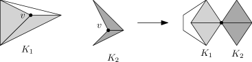
Figure 15: Transforming $K_{1}$ and $K_{2}$.

From the assumptions on links of vertices and from $K_{1}\neq K$ we deduce that the link of $v$ in $K_{1}$ is planar (and thus different from $S^{2}$). Indeed, if it were homeomorphic to $S^{2}$, then the link of $v$ in $K$ would not embed in $S^{2}$ since the link of $v$ in $K_{2}$ must be nonempty ($K_{2}\neq\{v\}$ since $K_{1}\neq K$). Similarly we can deduce that the link of $v$ in $K_{2}$ is planar.

Let $f_{1}\colon|K_{1}|\to S^{3}$ be a PL embedding. By the previous observation we deduce that $f_{1}(v)$ is on the boundary of $f_{1}(|K_{1}|)$. Therefore, there is a geometric simplex $\sigma$ in a small neighborhood of $f_{1}(v)$ such that $\sigma\cap f_{1}(|K_{1}|)=\{v\}$. Consequently, by the PL Schoenflies theorem (Corollary 12.4), there is a PL automorphism $\psi$ of $S^{3}$ mapping $\partial\sigma$ to $S^{2}\subset S^{3}$. In addition, we can assume that it maps the interior of $\sigma$ to the upper hemisphere of $S^{3}$ and $f_{1}(v)$ to a pre-chosen point $x$ on $S^{2}$. Altogether, $g_{1}:=\psi\circ f_{1}$ is a PL embedding mapping $|K_{1}|$ to the lower hemisphere of $S^{3}$ such that $g_{1}(|K_{1}|)\cap S^{2}=\{x\}$.

Similarly, we can find a PL map $g_{2}\colon|K_{2}|\to S^{3}$ such that $|K_{2}|$ is mapped to the upper hemisphere of $S^{3}$ and $g_{2}(|K_{2}|)\cap S^{2}=\{x\}$. Finally, we can construct the desired PL embedding $g$ of $|K|$ by setting $g(y):=g_{1}(y)$ if $y\in|K_{1}|$ and $g(y):=g_{2}(y)$ if $y\in|K_{2}|$. ∎

Proof of Lemma 12.2.

Clearly (i)$\Rightarrow$(ii), and (ii)$\Rightarrow$(iii) since $K^{\prime}$ is a subcomplex of a subdivision of $K$. It remains to show (iii)$\Rightarrow$(i).

Since $K^{\prime}$ is $2$-dimensional and since topological and PL embeddability coincide for embedding $2$-complexes in $S^{3}$, there is an PL embedding $f^{\prime}\colon|K^{\prime}|\to S^{3}$. Let $f_{0}$ be the restriction of $f^{\prime}$ to $|K^{(2)}|$ (which is a subspace of $|K^{\prime}|$). We want to extend $f_{0}$ to a PL embedding $f\colon|K|\to S^{3}$.

We will describe how to extend $f_{0}$ to each tetrahedron independently, and then we argue that these extensions can be done simultaneously, which yields the desired $f$. The argument is illustrated in Figure 16.

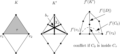
Figure 16: $K$, $K^{\prime}$ and $f(K^{\prime})$ schematically drawn in the plane.

Let $\tau$ be a tetrahedron of $K$. By the PL Schoenflies theorem (Corollary 12.4), $f_{0}(\partial\tau)$ splits the sphere $S^{3}$ in two open components whose closures are PL homeomorphic to $B^{3}$. Let $b_{\tau}$ be the barycentre of $\tau$ and let $C_{\tau}$ be the component that contains $f^{\prime}(b_{\tau})$. We will argue that $f_{0}(|K^{(2)}|)\cap C_{\tau}=\emptyset$.

Recall that $f_{0}(\partial\tau)$ is disjoint from $C_{\tau}$. For contradiction, let us assume that there is a component $C_{0}$ of $|K^{(2)}|\setminus\partial\tau$ such that $f_{0}(C_{0})\cap C_{\tau}\neq\emptyset$, that is $f_{0}(C_{0})\subseteq C_{\tau}$. Let $X_{\tau}:=|(\operatorname{sd}\tau)^{(2)}|\setminus|(\operatorname{sd}\partial\tau)|$. We have $f^{\prime}(X_{\tau})\subseteq C_{\tau}$ since $X_{\tau}$ is connected. Let $V_{0}$ be the set of those vertices $v$ of $\tau$ which belong to the closure of $C_{0}$. We have $|V_{0}|>0$ since $K$ is connected. Furthermore, $|V_{0}|>1$ since $K$ does not contain cut vertices. Therefore $|V_{0}|\geq 2$ and there is a path $P$ inside $|K^{(2)}|$ starting in a vertex $v_{1}$ of $\tau$, ending in a vertex $v_{2}$ of $\tau$, and with interior points in $C_{0}$.

Let $D$ be the subcomplex of $(\operatorname{sd}\tau)^{(2)}$, homeomorphic to a disk, consisting of the simplices in the plane of symmetry of $v_{1}$ and $v_{2}$ (considering $\tau$ as a regular simplex); it passes through the other two vertices of $\tau$ and the midpoint of $v_{1}v_{2}$. By a double application of the PL Schoenflies theorem and using that the interior of $|D|$ belongs to $X_{\tau}$ (which maps to $C_{\tau}$ under $f^{\prime}$), we have that $f^{\prime}(|D|)$ splits the closure of $C_{\tau}$ into two parts, both PL homeomorphic to a ball. Since $f_{0}(v_{1})$ and $f_{0}(v_{2})$ are in different parts, $f^{\prime}(|D|)\cap f_{0}(C_{0})\neq\emptyset$, which is impossible since $f^{\prime}$ is an embedding.

We have deduced that $f_{0}(|K^{(2)}|)\cap C_{\tau}=\emptyset$ for each tetrahedron $\tau$. By the PL Schoenflies theorem $f_{0}$ can be extended to a PL embedding of $K^{(2)}\cup\{\tau\}$ so that the interior of $\tau$ is mapped to $C_{\tau}$. Moreover, if we consider two distinct tetrahedra $\tau_{1},\tau_{2}\in K$, then $C_{\tau_{1}}\cap C_{\tau_{2}}=\emptyset$. Indeed, if $C_{\tau_{1}}\cap C_{\tau_{2}}\neq\emptyset$, then $C_{\tau_{1}}\subseteq C_{\tau_{2}}$ because $\partial C_{\tau_{2}}=f_{0}(\partial\tau_{2})$ is disjoint from $C_{\tau_{1}}$. Similarly we deduce $C_{\tau_{2}}\subseteq C_{\tau_{1}}$ implying $\partial C_{\tau_{1}}=\partial C_{\tau_{2}}$ contradicting the assumption that $\tau_{1}$ and $\tau_{2}$ are distinct simplices.

Altogether, we can extend $f_{0}$ to every tetrahedron of $K$ independently, obtaining the required PL embedding of $K$. ∎

References

- [AHT06] I. Agol, J. Hass, and W. Thurston. The computational complexity of knot genus and spanning area. Trans. Am. Math. Soc., 358(9):3821–3850, 2006.
- [Bac09] D. Bachman. Topological index theory for surfaces in 3-manifolds. Preprint arXiv:0901.0208, 2009.
- [Bac13] D. Bachman. Stabilizing and destabilizing Heegaard splittings of sufficiently complicated 3-manifolds. Mathematische Annalen, 355(2):697–728, 2013.
- [BDTS12] D. Bachman, R. Derby-Talbot, and E. Sedgwick. Almost normal surfaces with boundary. Preprint, arXiv:1203.4632, 2012.
- [Bin59] R. H. Bing. An alternative proof that 3-manifolds can be triangulated. Ann. Math. (2), 69:37–65, 1959.
- [Bin83] R. H. Bing. The geometric topology of -manifolds, volume 40 of American Mathematical Society Colloquium Publications. American Mathematical Society, Providence, RI, 1983.
- [ČKM+12] M. Čadek, M. Krčál, J. Matoušek, L. Vokřínek, and U. Wagner. Polynomial-time computation of homotopy groups and Postnikov systems in fixed dimension. Preprint, arXiv:1211.3093, 2012.
- [ČKM+13] M. Čadek, M. Krčál, J. Matoušek, F. Sergeraert, L. Vokřínek, and U. Wagner. Computing all maps into a sphere. J. ACM, 2013. To appear. Preprint in arXiv:1105.6257. Extended abstract in Proc. ACM–SIAM Symposium on Discrete Algorithms (SODA 2012).
- [ČKV13] M. Čadek, M. Krčál, and L. Vokřínek. Algorithmic solvability of the lifting-extension problem. Prepring, arXiv:1307.6444, 2013.
- [FM11] B. Farb and D. Margalit. A primer on mapping class groups. Princeton University Press. Princeton, NJ, 2011.
- [Fox48] R. H. Fox. On the imbedding of polyhedra in -space. Ann. of Math. (2), 49:462–470, 1948.
- [GHR13] J. Geelen, T. Huynh, and R. B. Richter. Explicit bounds for graph minors. Preprint, http://arxiv.org/abs/1305.1451, 05 2013.
- [GL89] C. McA. Gordon and J. Luecke. Knots are determined by their complements. J. Amer. Math. Soc., 2(2):371–415, 1989.
- [GR79] J.L. Gross and R.H. Rosen. A linear-time planarity algorithm for 2-complexes. J. Assoc. Comput. Mach., 20:611–617, 1979.
- [Hak61] W. Haken. Theorie der Normalflächen. Acta Math., 105:245–375, 1961.
- [Hat82] A. E. Hatcher. On the boundary curves of incompressible surfaces. Pacific J. Math., 99(2):373–377, 1982.
- [Hem76] J. Hempel. -Manifolds. Princeton University Press, Princeton, N. J., 1976. Ann. of Math. Studies, No. 86.
- [Hem79] G. Hemion. On the classification of homeomorphisms of -manifolds and the classification of -manifolds. Acta Math., 142(1-2):123–155, 1979.
- [HLP99] J. Hass, J. C. Lagarias, and N. Pippenger. The computational complexity of knot and link problems. J. ACM, 46(2):185–211, 1999.
- [Iva08] S. V. Ivanov. The computational complexity of basic decision problems in 3-dimensional topology. Geom. Dedicata, 131:1–26, 2008.
- [Jac80] W. Jaco. Lectures on three-manifold topology, volume 43 of CBMS Regional Conference Series in Mathematics. American Mathematical Society, Providence, R.I., 1980.
- [JO84] W. Jaco and U. Oertel. An algorithm to decide if a -manifold is a Haken manifold. Topology, 23(2):195–209, 1984.
- [JR03] W. Jaco and J. H. Rubinstein. -efficient triangulations of 3-manifolds. J. Differential Geom., 65(1):61–168, 2003.
- [JRS09] W. Jaco, J. H. Rubinstein, and E. Sedgwick. Finding planar surfaces in knot- and link-manifolds. J. Knot Theory Ramifications, 18(3):397–446, 2009.
- [JS03] W. Jaco and E. Sedgwick. Decision problems in the space of Dehn fillings. Topology, 42(4):845–906, 2003.
- [JT95] W. Jaco and J. L. Tollefson. Algorithms for the complete decomposition of a closed -manifold. Illinois J. Math., 39(3):358–406, 1995.
- [KMS13] M. Krčál, J. Matoušek, and F. Sergeraert. Polynomial-time homology for simplicial Eilenberg–MacLane spaces. J. Foundat. of Comput. Mathematics, 13:935–963, 2013. Preprint, arXiv:1201.6222.
- [Kup11] G. Kuperberg. Knottedness is in NP, modulo GRH. Preprint, arXiv:1112.0845, 2011.
- [Li10] Tao Li. Thin position and planar surfaces for graphs in the 3-sphere. Proc. Amer. Math. Soc., 138(1):333–340, 2010.
- [Mat97] S. V. Matveev. Classification of sufficiently large -manifolds. Uspekhi Mat. Nauk, 52(5(317)):147–174, 1997. Translation in Russian Math. Surveys 52 (1997), no. 5, 1029–1055.
- [Mat03] J. Matoušek. Using the Borsuk–Ulam theorem. Springer, Berlin etc., 2003.
- [MSTW13] J. Matoušek, E. Sedgwick, M. Tancer, and U. Wagner. Untangling two systems of noncrossing curves. Preprint, arXiv:1302.6475v3. Extended abstract in Proc. Graph Drawing 2013, 2013.
- [MTW11] J. Matoušek, M. Tancer, and U. Wagner. Hardness of embedding simplicial complexes in . J. Eur. Math. Soc., 13(2):259–295, 2011.
- [Neu68] L. Neuwirth. An algorithm for the construction of -manifolds from -complexes. Proc. Cambridge Philos. Soc., 64:603–613, 1968.
- [Pap43] C. Papakyriakopoulos. A new proof for the invariance of the homology groups of a complex (in Greek). Bull. Soc. Math. Grèce, 22:1–154 (1946), 1943.
- [RS72] C. P. Rourke and B. J. Sanderson. Introduction to piecewise-linear topology. Springer-Verlag, New York, 1972. Ergebnisse der Mathematik und ihrer Grenzgebiete, Band 69.
- [Rub95] J. H. Rubinstein. An algorithm to recognize the -sphere. In Proceedings of the International Congress of Mathematicians, Vol. 1, 2 (Zürich, 1994), pages 601–611, Basel, 1995. Birkhäuser.
- [Sch49] H. Schubert. Die eindeutige Zerlegbarkeit eines Knotens in Primknoten. S.-B. Heidelberger Akad. Wiss. Math.-Nat. Kl., 3:57–104, 1949.
- [Sch04] S. Schleimer. Sphere recognition lies in NP. Manuscript, available from http://www.warwick.ac.uk/~masgar, 2004.
- [Sko95] A. B. Skopenkov. A generalization of Neuwirth’s theorem on thickening -dimensional polyhedral. Mathematical Notes, 58(5):1244–1247, 1995.
- [Sto00] M. Stocking. Almost normal surfaces in -manifolds. Trans. Amer. Math. Soc., 352:171–207, 2000.
- [Tho94] A. Thompson. Thin position and the recognition problem for . Math. Res. Lett., 1(5):613–630, 1994.
- [Ton11] D. Tonkonog. Embedding 3-manifolds with boundary into closed 3-manifolds. Topology and its Applications, 158(9):1157–1162, 2011.