Analytical and Numerical Calculations for the Asymptotic Behaviors of Unitary $9j$ Coefficients

Abstract

Previously it was noted in numerical calculations that a certain unitary $9j$ coefficient

$$U(I,j)={\Big{<}(jj)^{2j}(jj)^{2j}\Big{|}(jj)^{2j}(jj)^{(2j-2)}\Big{>}}^{I}$$

decreases with increasing $j$ and for fixed small $I$. The decrease is of the form $Aj^{m}e^{-\alpha j}$. The exponential decay factor dominates. Analytically we also show using the Stirling approximation, that $\alpha=4\ln(2)$ and $m=\frac{3}{2}$.

1 Introduction

In previous works [1, 2] Zamick and Escuderos addressed the problem of maximum $j$-pairing. In the course of these studies they found that results simplified by the fact that a certain coupling matrix element was very small. This was the unitary $9j$ coefficient

$$U(I,j)={\Big{<}(jj)^{2j}(jj)^{2j}\Big{|}(jj)^{2j}(jj)^{(2j-2)}\Big{>}}^{I}$$ (1)

for small $I$ e.g. $I=2$. The work started in the $g_{9/2}$ shell. But as one went to higher shells this $U9j$ becomes rapidly smaller. Indeed behavior was parametrized as $Aj^{m}e^{-\alpha j}$ [2, 3]. The consequence of a very weak coupling is that for small total angular momentum $I$ the lowest 2 states for a maximum $J$ pairing interaction are ${\Big{<}(jj)^{2j}(jj)^{2j}\Big{|}(jj)^{J_{p}}(jj)^{J_{n}}\Big{>}}^{I}$ and ${\Big{<}(jj)^{2j}(jj)^{(2j-2)}\Big{|}(jj)^{J_{p}}(jj)^{J_{n}}\Big{>}}^{I}$ with $J_{p}$ and $J_{n}$ both even [1, 2]. In this work we will first conduct numerical studies to much higher angular momenta and with greater precision for the unitary $9j$ coefficients using Mathematica. We will then approach the problem analytically and derive the parameters $\alpha$ and $m$. We also consider cases where $I$ is large.

2 Calculation

2.1 Asymptotes of Small $I$

As was noted in [1] at first glance $U(2,j)$ seems to fall of exponentially with $j$. This suggests a form

$$Ae^{-\alpha j}$$ (2)

For this form $\ln(|U(2,j)|)=\ln(A)-\alpha j$. If this were true there would be a linear relationship between $\ln(|U(2,j)|)$ and $j$. We will here also consider other values of $I$ as indicated above.

We first plot, in Figure 1, $\ln(|U(I,j)|)$ vs $j$ for all even $I$ values between $I=2$ and $I=32$. The curves indeed approach straight lines indicating that the $U(I,j)$’s drops exponentially with $j$. This is certainly the dominant trend but there are small deviations indicated by the error analysis.

We try a more elaborate form

$$UA(I,j)=Aj^{m}e^{-\alpha j}$$ (3)

We consider the ratio

$$RR=\dfrac{\text{U}(I,j+1)^{2}}{\text{U}(I,j)\text{ }\text{U}(I,j+2)}$$ (4)

If we assume that $U9j=Aj^{m}e^{-\alpha j}$, then we have

$$RR=\dfrac{(A(j+1)^{m}e^{-\alpha(j+1)})^{2}}{Aj^{m}e^{-\alpha j}\times A(j+2)^{m}e^{-\alpha(j+2)}}$$ (5)

With some algebra this becomes

$$=\dfrac{e^{-2\alpha j}e^{-2\alpha}(j+1)^{2m}}{e^{-2\alpha j}e^{-2\alpha}j^{m}(j+2)^{m}}$$ (6)

It is obvious to see the factors which cancel out, then we take the ln of both sides and obtain

$$\ln(RR)=m\ln\left(\dfrac{(j+1)^{2}}{j(j+2)}\right)$$ (7)

We therefor have the extracted $m$

$$m=\dfrac{\ln(RR)}{\ln\left(\dfrac{(j+1)^{2}}{j(j+2)}\right)}$$ (8)

It should be noted that in the large $j$ limit $\dfrac{(j+1)^{2m}}{(j(j+2))^{m}}$ approaches $1+\dfrac{m}{j^{2}}$. We plot some cases of $m$ vs. $j$ in the attached Figures 3 to 4. We find that all even $I$ from $I=2$ to $I=12$, $m$ converges to 1.5 in the large $j$ limit.

It is important to note that in order to obtain the asymptotic value of $m$ in Eq.(3) one must go to a sufficiently large value of $j$. Furthermore the bigger the value of $I$ the higher one has to go in $j$. To show the perils of choosing the maximum $j$ too small suppose we choose it to by 500.5, which a priori most would consider to be a very large number. The values of $m$ for $I=2,4,10,20,30$ respectively 1.495, 1.481, 1.391, 1.085, and 0.577. We now see a steady decrease in $m$ as $I$ increases, which could lead to the false conclusion that there is a different asymptotic value of $m$ for each $I$. However when we choose $j$ large enough e.g. up to 7000.5 for $I=32$ we see that the asymptotic value of $m$ is the same for all even $I$ up to $I=32$, namely $m=1.5$. It should be noted that convergence is slower as $I$ increases.

2.2 Asymptotes of Large $I$

We next consider $U(I,j)$ for the largest values of $I$. We start with $I=I_{\text{max}}=4j-2$ and then also consider $I_{\text{max}}-2$, $I_{\text{max}}-4$, etc. We find that $U(I_{\text{max}},j)$ approaches a constant for large $j$ shown in Figure 6. We assume that the form of the asymptote is

$$U(I_{\text{max}}-2n,j)=\dfrac{A}{j^{n}}$$ (9)

Then we plot $U(I_{\text{max}}-2n,j)\times j^{n}$ versus $j$ to determine if this value approaches a constant. The results are shown in Figure 6. We can conclude then that the asymptote for large $I$ adheres to Eq.(9).

A formula involving many factorials for the case $I=I_{\text{max}}$ is also given by Varshalovich et al. in sec.10:8:4 Eq.(14) in [4]. We finally remind the reader that our motivation for this work comes from our desire to ether understand the wave function arising from a “maximum $J$-pairing” Hamiltonian [1, 2].

3 Analytical Results

3.1 Asymptotes of Small $I$

The numerical results in the previous section for the small $I$ cases lead to the result $m=1.5$ and the figures showed a dominantly exponential decrease with $j$ [3]. We can show some analytical results. We note that there is an explicit formula for the $9j$ symbol associated with the unitary $9j$ coefficient above in the work of Varshalovich et al. [4] sec 10:8:3 Eq.(9) shown here:

$$9j=\left\{\begin{array}[]{ccc}a&b&c\\ d&e&f\\ a+d&b+e&j\end{array}\right\}=\left<cf\text{ }(a-b)(d-e)|j(a-b+d-e)\right>$$

$$\times\left[\dfrac{(2a)!(2b)!(2d)!(2e)!(a+b+d+e+j+1)!(a+d+e+b-j)!}{(2a+2d+1)!(2b+2e+1)!(a+b+c+1)!(a+b-c)!(d+e+f+1)!(d+e-f)!(2j+1)}\right]^{\frac{1}{2}}$$ (10)

We associate $a,b,d,e\rightarrow j$; $c,(a+d),(b+e)\rightarrow 2j$; $f\rightarrow(2j-2)$; and $j\rightarrow I$. For some simplification we define a new variable $J=2j$. We apply that expression to this problem and consider $U9j$ rather than $9j$,

$$U(I,j)=\dfrac{(J!)^{2}}{(2J)!}\left[\dfrac{(2J+I+1)!(2J-I)!(2J+1)(2J-3)}{(2J+1)!(2J-1)!}\right]^{\frac{1}{2}}\times\sqrt{\dfrac{1}{2(2I+1)}}\times\left<J(J-2)00|I0\right>$$ (11)

Thus we have related the $U9j$ to a Clebsch-Gordan(CG) coefficient.

For the particular $U9j$ above and for $I=2$ we obtain the following expression

$$U(2,j)=\dfrac{(J!)^{2}}{(2J)!}\left[\dfrac{(2J+1)(2J+3)(2J+2)(2J-3)}{(2J-1)}\right]^{\frac{1}{2}}\times\sqrt{\dfrac{1}{10}}\times\left<J(J-2)00|20\right>$$ (12)

This special $U9j$ is proportional to a Clebsch-Gordan coefficient. There is a useful formula in Talmi’s book [5] for the associated $3j$ symbol shown here:

$$\left(\begin{array}[]{ccc}j_{1}&j_{2}&j_{3}\\ 0&0&0\end{array}\right)=\dfrac{1}{2}\left(1+(-1)^{j_{1}+j_{2}+j_{3}}\right)(-1)^{g}\times\sqrt{\dfrac{(2g-2j_{1})!(2g-2j_{2})!(2g-2j_{3})!}{(2g+1)!}}\times\dfrac{g!}{(g-j_{1})!(g-j_{2})!(g-j_{3})!}$$ (13)

where $2g=j_{1}+j_{2}+j_{3}$ and

$$CG=\mathchoice{{\hbox{$\displaystyle\sqrt{(2j_{3}+1)\,}$}\lower 0.4pt\hbox{\vrule height=7.5pt,depth=-6.00003pt}}}{{\hbox{$\textstyle\sqrt{(2j_{3}+1)\,}$}\lower 0.4pt\hbox{\vrule height=7.5pt,depth=-6.00003pt}}}{{\hbox{$\scriptstyle\sqrt{(2j_{3}+1)\,}$}\lower 0.4pt\hbox{\vrule height=5.25pt,depth=-4.20003pt}}}{{\hbox{$\scriptscriptstyle\sqrt{(2j_{3}+1)\,}$}\lower 0.4pt\hbox{\vrule height=3.75pt,depth=-3.00002pt}}}(-1)^{j_{1}-j_{2}}\left(\begin{array}[]{ccc}j_{1}&j_{2}&j_{3}\\ 0&0&0\end{array}\right)$$ (14)

There is a simpler formula in Talmi’s book [5] for this coefficient when $I=2$:

$$\left<J(J-2)00|20\right>=-\sqrt{\dfrac{15J(J-1)^{2}}{((2J-3)(2J-2)(2J-1)(2J+1))}}$$ (15)

It is easy to see that the CG coefficient falls off as $\dfrac{1}{\sqrt{J}}$. We now get the combined expression

$$U(2,j)=\dfrac{(J!)^{2}}{(2J)!}\sqrt{\dfrac{3J(J-1)^{2}(2J+3)(2J+2)}{2(2J-2)(2J-1)^{2}}}$$ (16)

The exponential behavior comes from the factorials via the Stirling approximation

$$\ln(n!)\approx n\ln(n)-n$$ (17)

If we stop there we get

$$\ln\left(\dfrac{(J!)^{2}}{(2J)!}\right)\approx 2J\ln(J)-2J\ln(2J)=-2J\ln 2$$ (18)

However to get the correct asymptotic behavior we must go beyond this and include one more term to obtain the more accurate Stirling approximation

$$\ln(n!)=n\ln(n)-n+\ln(\sqrt{2\pi n})$$ (19)

Using the extended Stirling approximation this becomes

$$\ln\left(\dfrac{(J!)^{2}}{(2J)!}\right)\approx-2J\ln(2)+\ln(\sqrt{\pi J})$$ (20)

Recall that we had assigned $J=2j$ and then taking a inverse logarithm of this yields a contribution

$$\dfrac{(J!)^{2}}{(2J)!}\approx e^{-4\ln(2)j}\sqrt{2\pi j}$$ (21)

When we go from $j$ to $j+1$ we get a decreases of about 16 from the exponential factor. This decrease dominates over the increase from the second factor. The second factor and the other terms must contribute to get the $j^{m}$ part which serves to reduce this ratio a bit.

If the “small” term in the Stirling approximation is neglected a problem arises. The factors under the square root sign clearly go as $j^{3/2}$ in the large $j$ limit. However the Clebsch-Gordan coefficient decreases with $j$. This leads to an effective $m$ less than $\frac{3}{2}$. However numerical calculations [3] clearly indicate that $m=\frac{3}{2}$. Hence, although the simplest version of the Stirling approximation gives the right exponential behavior it gives the wrong $j^{m}$ dependence. By including the “small correction” we take care of this problem.

Analytic expressions of specific $9j$ coefficients have been previously considered for special cases e.g. for the case of partial dynamical symmetries by Robinson and Zamick [6]. Many relations for $9j$ symbols were found by Zhao and Arima [7] in the context of maximum $j$-pairing hamiltonians. Explicit studies of the asymptotic behavious of $9j$ coefficients have been performed by Anderson et. al. [8] and by Yu and Littlejohn [9]. What distinguishes the present work from the ones just mentioned is that only here do we consider $9j$s which display an exponential decrease with increasing $j$. This is called non-classical behavior by the experts. The large difference in behavior comes from the fact that we are considering coupling matrix elements involving 2 different $J$ values $2j$ and $2j-2$ whereas in Zhao and Arima [7] for the problem they are addressing they have the same $J$ values. Ironically we have to be in the non-classical region mathematically to reach the classical limit for the physical problem in question.

3.2 Asymptotes of Large $I$

We now consider the region near $I=I_{\text{max}}=4j-2$. It should be pointed out that whereas in the small $I$ case we kept $I$ fixed as we increased $j$, here as we change $j$ we change $I$. Thus we are making different comparisons. The figures confirm that for this analysis there is a power law behavior rather than an exponential one. The $U9j$ goes as $\dfrac{1}{j^{n}}$ where $n=\dfrac{(I_{\text{max}}-I)}{2}$. It should be noted that for $I=I_{\text{max}}=4j-2$ the value of the $U9j$ was shown by Talmi [10] to be

$$U9j=\dfrac{\sqrt{(2j-1)(8j-1)}}{(8j-2)}$$ (22)

Note that this 9j approaches 1/2 when j becomes very large. Subsequently an alternate proof was provided by Bayman[11].

For large $I$ we write $I=4j-2-2n$ and assume $n$ is much smalller than $j$. We use a more general formula in Talmi’s book [5] (top of page 960) for $\big{<}2j(2j-2)00\big{|}I0\big{>}$.

We can get an expression for all $n$ by using the Stirling approximation for factorials involving large parameters but not for those involving only $n$. We obtain the following result:

$$U9j=\dfrac{(-1)^{n}}{2\mathchoice{{\hbox{$\displaystyle\sqrt{2\,}$}\lower 0.4pt\hbox{\vrule height=6.44444pt,depth=-5.15558pt}}}{{\hbox{$\textstyle\sqrt{2\,}$}\lower 0.4pt\hbox{\vrule height=6.44444pt,depth=-5.15558pt}}}{{\hbox{$\scriptstyle\sqrt{2\,}$}\lower 0.4pt\hbox{\vrule height=4.51111pt,depth=-3.6089pt}}}{{\hbox{$\scriptscriptstyle\sqrt{2\,}$}\lower 0.4pt\hbox{\vrule height=3.22221pt,depth=-2.57779pt}}}16^{n}}\dfrac{\sqrt{\left((2n+2)!(2n)!\right)}}{(n!)j^{n}}$$ (23)

as $j$ becomes very large. One can verify that for $n=0$ this is indeed $\dfrac{1}{2}$ and note that for $n=1$ we get $\dfrac{\sqrt{3/2}}{8j}$. One notes that in this limit ($n$ much smaller than $j$) the Clebsch-Gordan coefficient goes as $\dfrac{1}{j^{1/4}}$ (alternatively the $3j$ goes as $\dfrac{1}{j^{3/4}}$) in the large $j$ limit. In more detail we have:

$$CG=\dfrac{\sqrt{(2n)!}}{n!(2^{n})}\left(\dfrac{1}{\pi j}\right)^{1/4}(-1)^{n}$$ (24)

The $\dfrac{1}{j^{1/4}}$ behavior in the large $I$ limit is in contrast to the behavior in the previous section where $I$ was fixed at a small value whilst $j$ was increased. In that case the Clebsch-Gordan coefficient from Eq.(14) went as $\dfrac{1}{j^{1/2}}$. In this work our motivation for studying the specific $U9j$ coefficients above, was to better understand the wave functions of a maximum $J$-pairing hamiltonian. What we had previously shown numerically we now have attempted to show analytically. We found the numerical results crucial in guiding us to the analytical ones. We have succeeded in getting analytic expressions for the asymptotic behaviors for small $I$ by using the extended Stirling approximation. We are also able to make statements about the large $I$ problem.

We would like to thank Ben Bayman and Igal Talmi for their valuable help and interest.

Brian Kleszyk also thanks the Rutgers Aresty Research Center for undergraduate research for support during the 2013-2014 academic year.

Appendix A Appendix

In this paper we focus on equations (11 and 13), and (23 and 24) of the work of Kleszyk and Zamick [3]. In particular we consider the case when the total angular momentum $I$is equal to $I_{\text{max}}-2n$ and $I_{\text{max}}\equiv 4j-2$, and $n=0,1,2,...$ We take the limit of large $j$ where $n$ becomes much smaller than $j$. We also define $J=2j$, where $j$ is the .We first address the 3$j$ coefficient:

$$\left(\begin{array}[]{ccc}2J&2J-2&I\\ 0&0&0\end{array}\right)$$ (25)

We then also can define $I$ using a new variable $m$ with $I=4j-2m$, and this time $m=1,2,3,...$ We can separate parts of the 3$j$ which now becomes

$$3j=\dfrac{\sqrt{(2m-1)!}}{(m-1)!}(-1)^{m}\sqrt{\dfrac{N_{1}!N_{2}!}{N_{3}!}}\dfrac{N_{4}!}{N_{5}!N_{6}!}$$ (26)

where the 6 factors $N_{i}$ are:

$$\begin{array}[]{ccc}N_{1}=2J-2-2m&N_{2}=2J+2-2m&N_{3}=4J-1-2m\\ N_{4}=2J-1-m&N_{5}=J-1-m&N_{6}=J+1-m\end{array}$$ (2a)

We use the Stirling approximation,

$$\ln N!=N\ln N-N+\ln\sqrt{2\pi N}$$ (27)

and it should be noted that the approximation approaches the true value asymptotically. Now we can write: $N_{i}=(\alpha_{i}+\beta_{i}m+\gamma_{i}J)$ with differing constant coefficients. In Eq.(2a) we give the contribuition of $-N,\ln\sqrt{2\pi N},\alpha\ln N,m\beta\ln N,$ and $\gamma J\ln N$. For the latter we break things up into (a)“extreme” and (b) “next order”. This is necessary because “next order” has contriutions comparable to those in “$-N$”.

Table 1: Asymptotic contributions to the 3j coefficients

	$-N_{i}$	$\ln\sqrt{2\pi N_{i}}$	$\alpha_{i}\ln N_{i}$
(1)	$\dfrac{}{}-\frac{1}{2}(2J-2-2m)$	$\frac{1}{2}\ln\sqrt{4\pi J}$	$-\ln(2J)$
(2)	$\dfrac{}{}-\frac{1}{2}(2J+2-2m)$	$\frac{1}{2}\ln\sqrt{4\pi J}$	$-\ln(2J)$
(3)	$\dfrac{}{}\frac{1}{2}(4J-1-2m)$	$\frac{1}{2}\ln\sqrt{4\pi J}$	$-\ln(2J)$
(4)	$\dfrac{}{}\frac{}{}-(2J-1-m)$	$\frac{1}{2}\ln\sqrt{4\pi J}$	$-\ln(2J)$
(5)	$\dfrac{}{}(J-1+m)$	$\frac{1}{2}\ln\sqrt{4\pi J}$	$-\ln(2J)$
(6)	$\dfrac{}{}(J+1-m)$	$\frac{1}{2}\ln\sqrt{4\pi J}$	$-\ln(2J)$
Total	$\dfrac{}{}\frac{1}{2}$	$\ln\left(\frac{2}{\pi J}\right)^{1/4}$	$\ln\frac{1}{\sqrt{J}}$

(a)

	$\beta_{i}m\ln N_{i}$	$\gamma_{i}J\ln N_{i}$	$\gamma_{i}J\ln N_{i}$
(1)	$\dfrac{}{}-m\ln(2J)$	$J\ln J$	$-1-m$
(2)	$\dfrac{}{}-m\ln(2J)$	$-J\ln(2J)$	$1-m$
(3)	$\dfrac{}{}m\ln(4J)$	$-2J\ln(2J)$	$\frac{1}{2}+m$
(4)	$\dfrac{}{}-m\ln(2J)$	$2J\ln(2J)$	$-1-m$
(5)	$\dfrac{}{}m\ln J$	$-J\ln J$	$1+m$
(6)	$\dfrac{}{}m\ln J$	$-J\ln J$	$-1+m$
Total	$\dfrac{}{}-m\ln 2$	$0$	$-\frac{1}{2}$

(b)

First notice that “$\gamma J\ln N$” result is $\dfrac{1}{2}$, which cancels the $+\dfrac{1}{2}$ from “$-N$”. Adding up all the totals we get

$$-m\ln 2+\ln\left(\dfrac{2}{\pi J}\right)^{1/4}+\ln\left(\dfrac{1}{\sqrt{J}}\right)$$ (28)

$$=-m\ln 2+\ln\left(\dfrac{2}{\pi J^{3}}\right)^{1/4}$$ (29)

Taking the antilog we get

$$3j\approx e^{m\ln 2}\left(\dfrac{2}{\pi J^{3}}\right)^{1/4}$$ (30)

and note that $e^{-m\ln 2}=\dfrac{1}{2^{m}}$.

Putting everything together and putting things in terms of $j$ and $n$ we obtain

$$3j\rightarrow\dfrac{\sqrt{(2n)!}}{n!2^{n}}(-1)^{n}\left(\dfrac{1}{64\pi j^{3}}\right)^{1/4}$$ (31)

We see that in the limit $n\ll j$, $3j$ goes as $\dfrac{1}{j^{3/4}}$. Alternatively the Clebsch-Gordan has an asymptotic value

$$CG\rightarrow\dfrac{\sqrt{(2n)!}}{n!2^{n}}(-1)^{n}\left(\dfrac{1}{\pi j}\right)^{1/4}$$ (32)

A.1 The Unitary $9j$ coefficient

Again we will write $I=4j-2m$, with $m=1,2,3,...$ and we can rewrite Eq.(11) from [3] as

$$U(9j)=\dfrac{FAC}{\sqrt{PROD}}\sqrt{\dfrac{(2J+1)(2J-3)}{2}}\times 3j$$ (33)

where

$$FAC=\dfrac{(C_{1}!)^{2}}{C_{2}!}\sqrt{\dfrac{C_{3}!}{C_{4}!C_{5}!}}$$ (34)

with

$$\begin{array}[]{rrrrr}C_{1}=J&C_{2}=2J&C_{3}=4-J+1&C_{4}=2J+1&C_{5}=2J-1\end{array}$$

Then we also have

$$PROD=(4J+1)(4J)...(4J-m)$$ (35)

There are $2m$ terms in $PROD$. Asymptotically we obtain

$$\sqrt{\dfrac{(2J+1)(2J-3)}{2}}\rightarrow\sqrt{2J}$$ (36)

$$PROD\rightarrow(4J)^{2m}=(8j)^{2m}$$ (37)

Hence we have

$$\dfrac{1}{\sqrt{PROD}}\rightarrow\dfrac{1}{(8j)^{m}}$$ (38)

We use the Stirling approximation to calculate $FAC$. The detailed results are given in Table 2.

Table 2: $\ln\dfrac{(C_{1}!)^{2}}{C_{2}!}\dfrac{C_{3}!}{C_{4}!C_{5}!}$

	$-C_{i}$	$\ln\sqrt{2\pi C_{i}}$	$\alpha_{i}\ln C_{i}$	$\gamma_{i}J\ln()$	$\gamma_{i}J\ln()$
(1)	$\dfrac{}{}-2J$	$2\ln(\sqrt{2\pi J})$	$0$	$2J\ln J$	$0$
(2)	$\dfrac{}{}+2J$	$-\ln\sqrt{4\pi J}$	$0$	$-2J\ln(2J)$	$0$
(3)	$\dfrac{}{}-2J-\frac{1}{2}$	$\ln\sqrt{8\pi J}$	$\frac{1}{2}\ln(4J)$	$2J\ln(4J)$	$\frac{1}{2}$
(4)	$\dfrac{}{}J+\frac{1}{2}$	$-\frac{1}{2}\ln\sqrt{4\pi J}$	$-\frac{1}{2}\ln(2J)$	$-J\ln(2J)$	$\frac{1}{2}$
(5)	$\dfrac{}{}-J-\frac{1}{2}$	$-\frac{1}{2}\ln\sqrt{4\pi J}$	$\frac{1}{2}\ln(2J)$	$-J\ln(2J)$	$-\frac{1}{2}$
Total	$\dfrac{}{}-\frac{1}{2}$	$\ln(\frac{\pi J}{2})^{1/4}$	$\ln(2\sqrt{J})$	$0$	$\frac{1}{2}$

A.2 Combing Table 1 and Table 2

There are many cancellations when we add the totals of $\ln FAC$ and $\ln 3j$ in Table 1 and Table 2. The result is

$$\ln FAC+\ln 3j=-(m-1)\ln 2=-n\ln 2$$ (39)

The antilog is

$$e^{-n\ln 2}=\dfrac{1}{2^{n}}$$ (40)

All the $j$ dependance The $j$ dependence comes from

$$\sqrt{\dfrac{(2J+1)(2J-3)}{2}}$$ (41)

and PROD

$$\sqrt{PROD}\rightarrow(8j)^{m}$$ (42)

putting everything together we obtain the result:

$$U9j\rightarrow\dfrac{(-1)^{n}}{2\sqrt{2}16^{n}}\dfrac{\sqrt{\left((2n+2)!(2n)!\right)}}{(n!)j^{n}}$$ (43)

We note other work on asymptotics of CG coefficients by Reinsch and Morehead [12]. In their work they define

$$\beta=((j_{1}+j_{2}-j)(j+j_{2}-j_{1})(j+j_{1}-j_{2})(j_{1}+j_{2}+j))^{1/2}$$ (44)

They find an approximate expression for the CG coeffecients in their Eq.(B9).

$$CG=\left<j_{1}j_{2}00|j0\right>\approx 2(-1)^{\frac{j_{1}+j_{2}-j}{2}}\sqrt{\dfrac{2j+1}{2\pi\beta}}\sqrt{\dfrac{j+j_{1}+j_{2}}{j+j_{1}+j_{2}+1}}(1+\delta_{4}+\delta_{6})$$

$$\times\left[1+\dfrac{1}{24}\left(\dfrac{2}{j}+\dfrac{2}{j_{1}}+\dfrac{1}{j_{2}}-\dfrac{1}{j+j_{1}+j_{2}}-\dfrac{1}{-j+j_{1}+j_{2}}-\dfrac{1}{j-j_{1}+j_{2}}-\dfrac{1}{j+j_{1}-j_{2}}\right)\right]$$ (45)

We quickly run into trouble in making a comparison with our results, especially for $n=0$. In their Eq.(B12) they have in the leading term CG proportional to $\dfrac{1}{\sqrt{\beta}}$. However for the case $j=j_{1}+j_{2}$, that is to say $I=I_{max}$, with our $n=0$, we see that $\beta$ vanishes and hence their expression for CG blows up. Evidently their formula is not valid in this region. On the other hand our expression Eq.(13) from [3] works just fine.

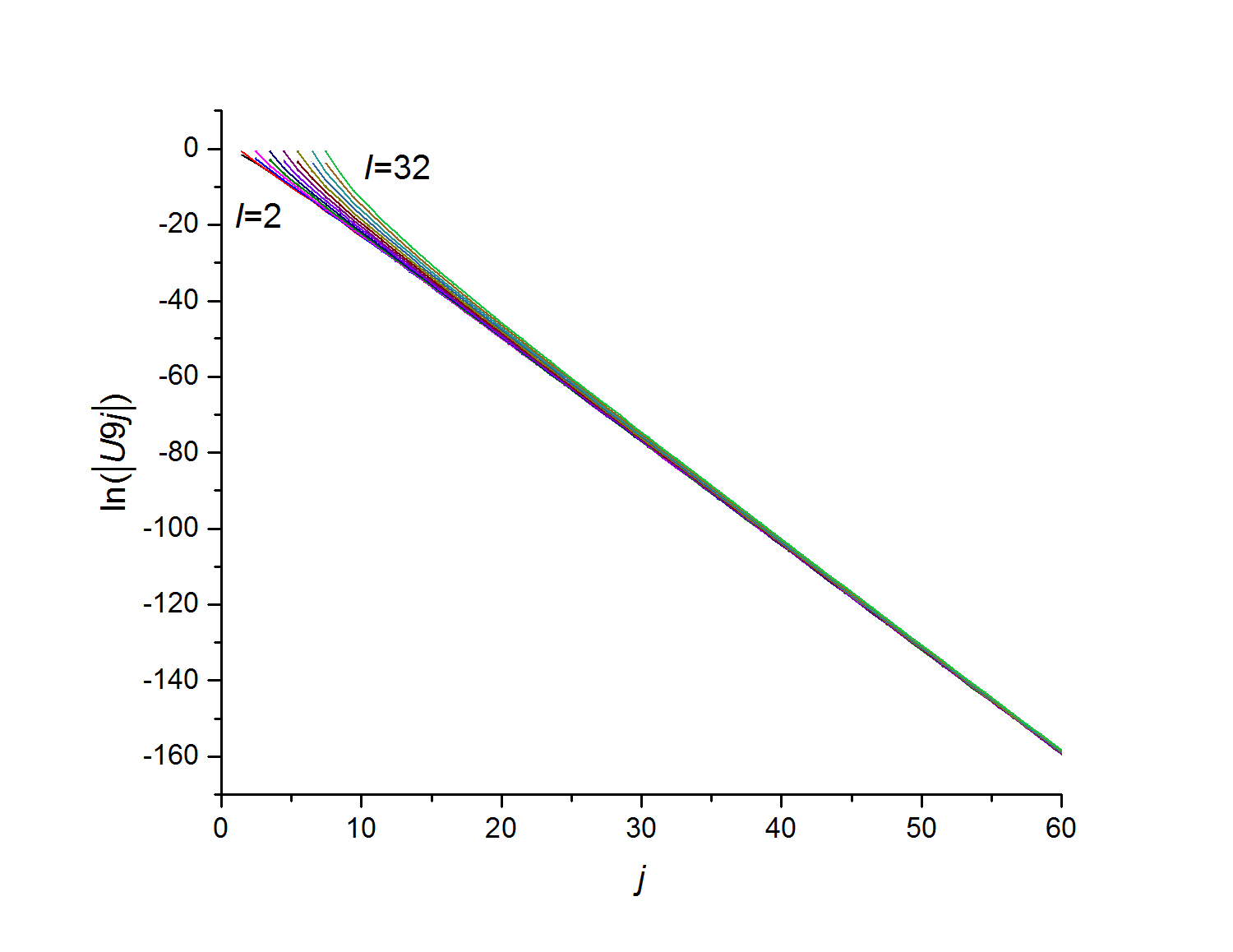
Figure 1: (color online)$\ln(|U9j|)$ vs $j$
$I=2,4,6,...,32$

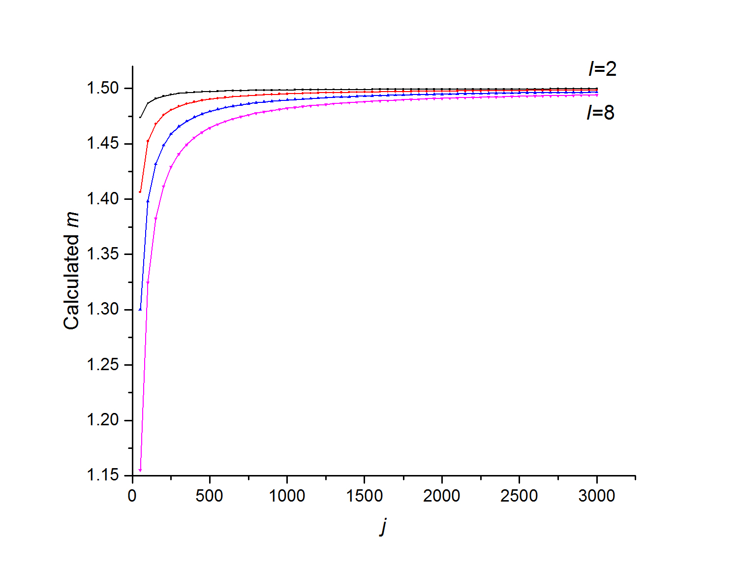
Figure 2: (color online)Suspected $m$ vs $j$
$I=2,4,6,8$

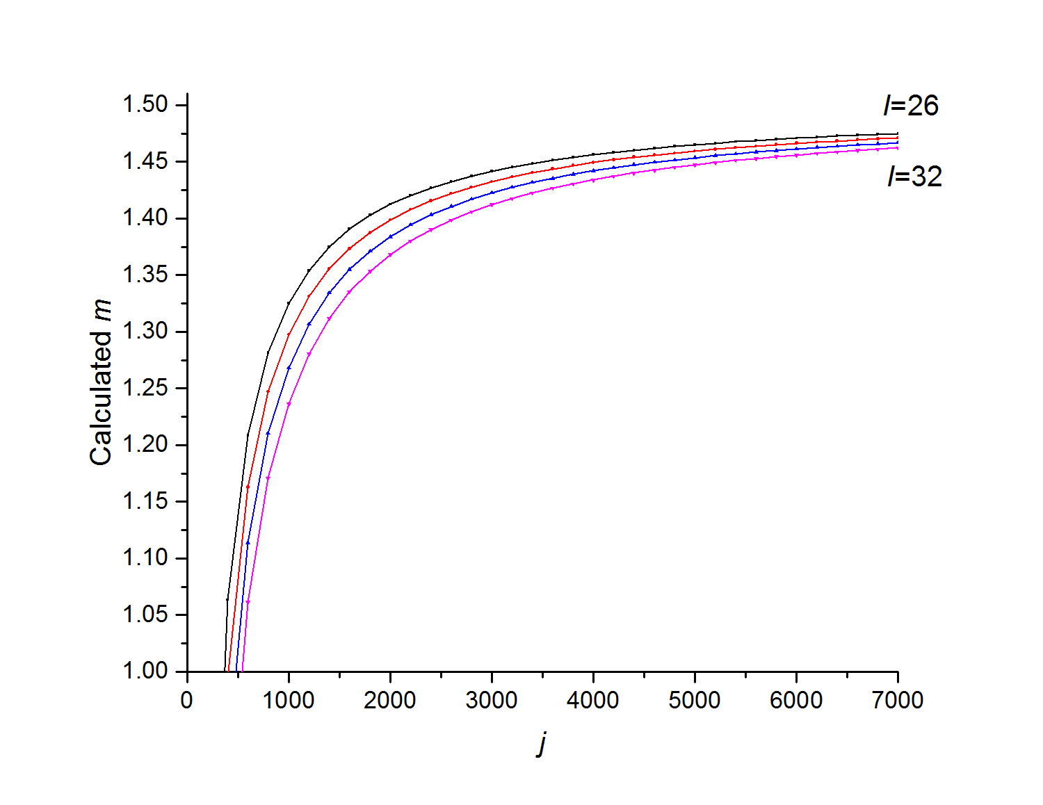
Figure 3: (color online)Suspected $m$ vs $j$
$I=26,28,30,32$

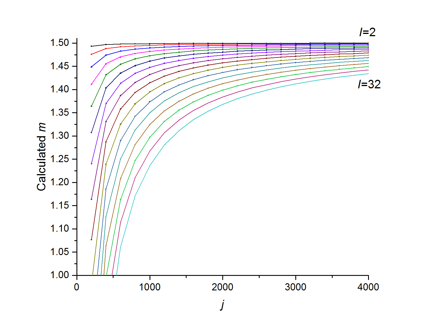
Figure 4: (color online)Suspected $m$ vs $j$
$I=2,4,6,...,32$

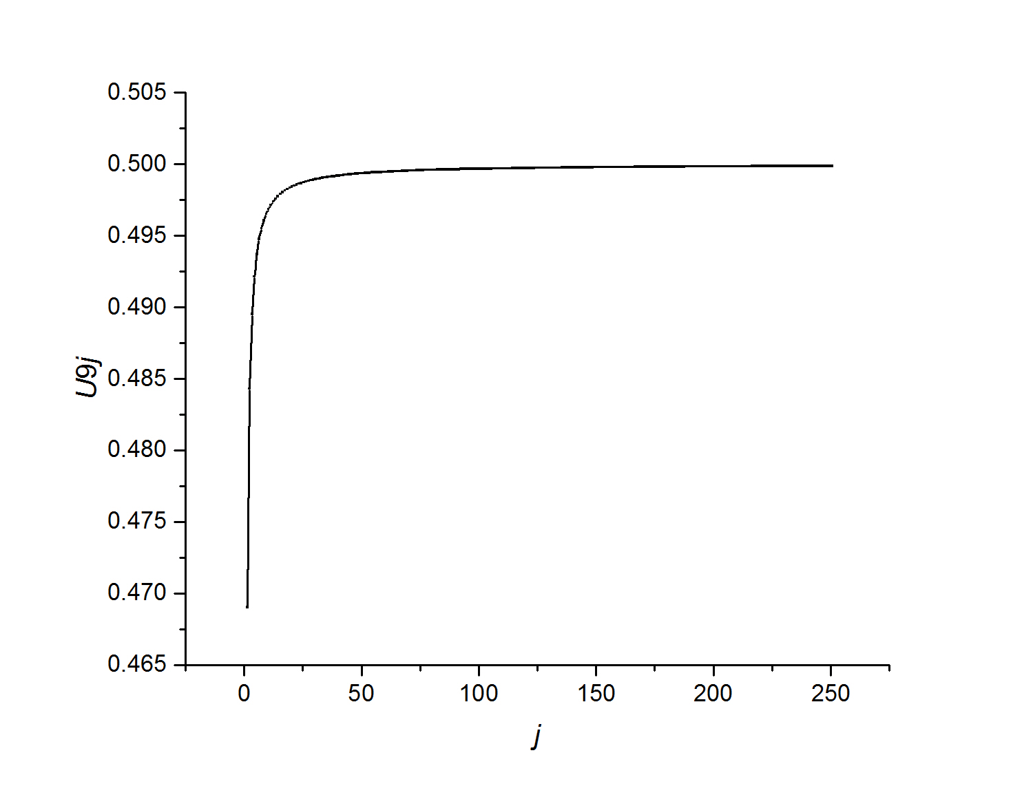
Figure 5: (color online)$U9j$ vs $j$, $I=I_{\text{max}}$
$(n=0)$

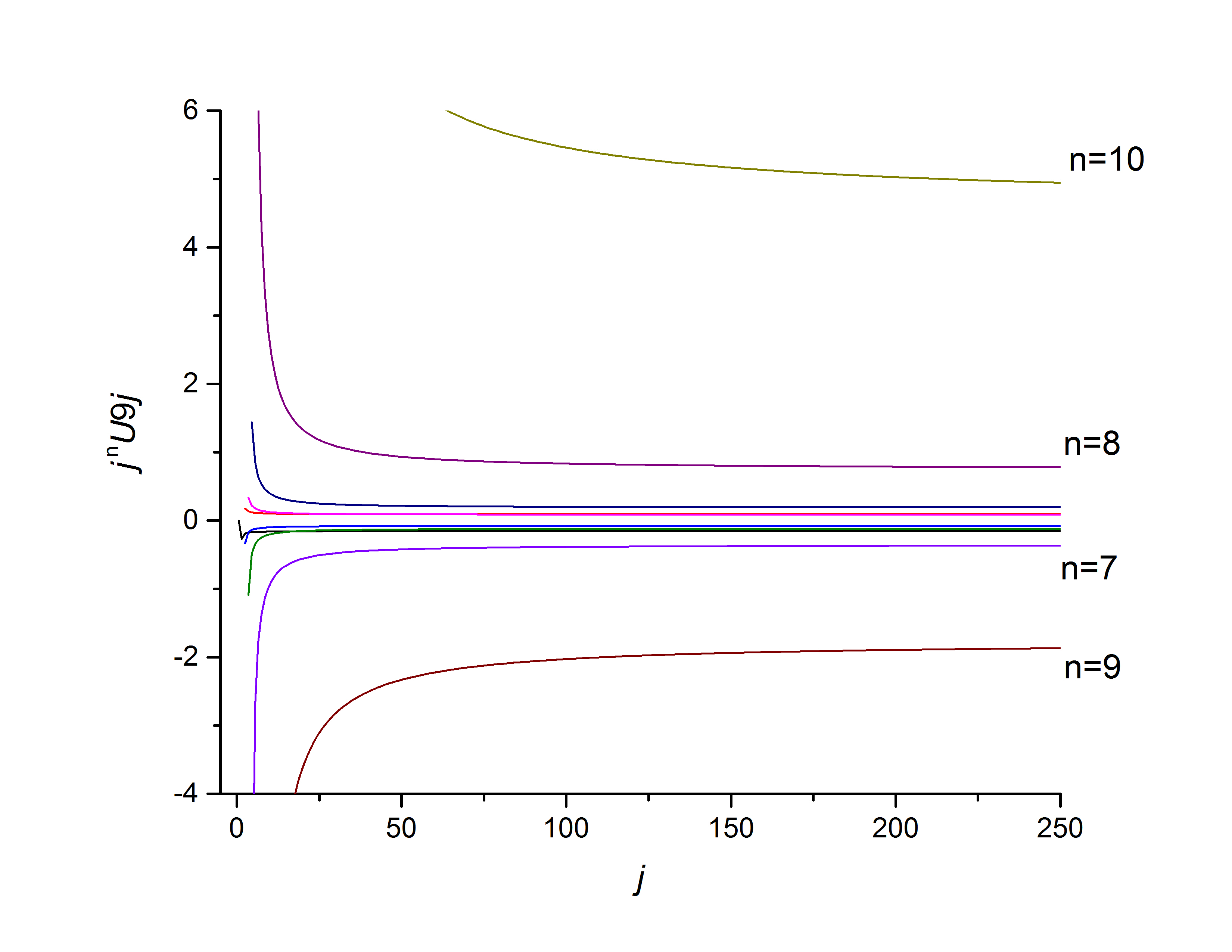
Figure 6: (color online)$(j^{n}U9j)$ vs $j$, $I=I_{\text{max}}-2n$
$n=1,2,...,10$

References

[1] L. Zamick and A. Escuderos, Phys. Rev. C 87,044302
(2013).
[2] L. Zamick and A. Escuderos, Phys. Rev. C 88,014326
(2013).
[3] B. Kleszyk and L. Zamick, Phys. Rev. C 89,044322 (2014)
[4] D.A. Varshalovich, A. N. Moskalev and V.K.
Khersonskiĭ (1988) Quantum Theory of Angular Momentum,
World Scientific Publishing Co. Inc., Singapore.
[5] Igal Talmi, Simple Models of Complex Nuclei, Harwood
Academic Publishers, Switzerland
[6] S.J.Q. Robinson and L. Zamick Phys.Rev C64 (2001)
057302
[7] Y.M. Zhao and A. Arima, Phys Rev. C72, 054307 (2005)
[8] R.W. Anderson, V. Aquilanti and C. da Silva Ferreira,
J, Chem. Phys. 129,161101 (2008)
[9] L. Yu and R.C.L. Littlejohn, Phys. Rev. a83,062114 (2011)
[10] Igal Talmi, private communication.
[11] Ben Bayman, private communication.
[12] M.W. Reinsch and J.J. Morehead, arXiv:math-ph/9906007v2, 26 Jul 1999