Analytical approach for the approximation solution of the independent DGLAP evolution equations with respect to the hard Pomeron Behavior

Abstract

We show that it is possible to use hard-Pomeron behavior to the gluon distribution and singlet structure function at low $x$. We derive a second-order independent differential equation for the gluon distribution and the singlet structure function. In this approach, both singlet quarks and gluons have the same high-energy behavior at small $x$. These equations are derived from the next-to-leading order DGLAP evolution equations. All results can be consistently described in the framework of perturbative QCD, which shows an increase of gluon distribution and singlet structure functions as $x$ decreases.

The DGLAP $[1]$ evolution equations are fundamental tools to study the $Q^{2}$ and $x$ evolutions of structure functions, where $x$ is the Bjorken scaling and and $Q^{2}$ is the four momenta transfer in a deep inelastic scattering (DIS) process $[2]$. The measurements of the $F_{2}(x,Q^{2})$ structure functions by DIS processes in the small- $x$ region have opened a new era in parton density measurements inside hadrons. The structure function reflects the momentum distributions of the partons in the nucleon. It is also important to know of the gluon distribution inside a hadron at low- $x$ because gluons are expected to be dominant in this region. The steep rise of $F_{2}(x,Q^{2})$ towards low $x$ observed at HERA also indicates in perturbative quantum chromodynamics (PQCD) a similar rise of the gluon distribution towards low $x$. In the usual procedure the DIS data are analyzed by the NLO QCD fits based on the numerical solution of the DGLAP evolution equations and it is found that the DGLAP analysis can well describe the data in the perturbative region $Q^{2}{\geq}1GeV^{2}$ [3]. As a alternative to the numerical solution, one can study the behavior of the quarks and gluons through the analytical solutions of the evolution equations. Although exact analytic solutions of the DGLAP equations are not possible in the entire range of $x$ and $Q^{2}$, such solutions are possible under certain conditions [4-5] and are then quite then successful as far as the HERA small $x$ data are concerned.
Small $x$ behavior of structure functions for fixed $Q^{2}$ reflects the high energy behavior of the virtual Compton scattering total cross section with increasing the total center-of-mass energy squared $W^{2}$ becuse $W^{2}=Q^{2}(1/x-1)$. The appropriate framework for the theoretical description of this behavior is the Regge pole exchange picture [6]. It can be asserted confidently that Regge theory is one of the most successful approaches to the description of high energy scattering of hadrons. This high energy behavior can be described by two contributions: an effective Pomeron with its intercept slightly above unity ($\sim$1.08) and the leading meson Regge trajectories with intercept $\alpha_{R}(0){\approx}0.5$ [7]. The hypothesis of the Pomeron with data of the total cross section shows that a better description is achieved in alternative models with the Pomeron having intercept one, but with a harder $j$ singularity (a double pole) [8]. This model has two Pomeron components, each of them with intercept $\alpha_{P}=1$; one is a double pole and the other one is a simple pole [9]. It is tempting, however, to explore the possibility of obtaining approximate analytical solutions of DGLAP equations themselves in the restricted domain of low- $x$ at least. Approximate solutions of DGLAP equations have been reported $[10-12]$ with considerable phenomenological success. In such an approximate scheme, one uses a Taylor expansion valid at low- $x$ and reframes the DGLAP equations as partial differential equations in the variable $x$ and $Q^{2}$ which can be solved by standard methods.
In the past three decades, some authors were the first to report a detailed look at the Regge input into the DGLAP equations [13-15]. So that we have shown [16-19] that it was possible to use Regge- like behavior as an input for the Dokshitzer-Gribov-Lipatov-Altarelli-parisi(DGLAP) evolution equations at low $x$. The small $x$ region of the Deep inelastic electron- proton scattering(DIS) offers a unique possibility to explore the Regge limit of perturbative quantum chromodynamic(PQCD)[6]. This model gives the following parametrizations of the DIS distribution functions, $f_{i}(x,Q^{2})=A_{i}(Q^{2})x^{-\lambda_{i}}$ (i=$\Sigma$(singlet structure function) and g(gluon distribution)), where $\lambda_{i}$ is Pomeron intercept minus one, show that $\lambda_{i}=dlnf_{i}(x,Q^{2})/dln1/x$ definitely rises with $Q^{2}$. In the present article we concentrate on the Regge behavior in our calculations, although good fits to the results clearly show that the gluon distribution and the singlet structure function need a model with a hard Pomeron. In such scheme, one uses this behavior that is valid at low $x$ and reframes the DGLAP evolution equations as independent partial differential equations in the variables $x$ and $Q^{2}$, which can be solved by standard methods. Also, we should be able to calculate $\lambda_{s}$ and $\lambda_{g}$ in the next- to-leading order(NLO) DGLAP equations.

The NLO- DGLAP equations for the evolution of the singlet structure function and the gluon distribution can be written as

$$\frac{dG(x,Q^{2})}{dlnQ^{2}} = \frac{\alpha_{s}}{2\pi}{\int_{0}^{1-x}}dz[P^{LO+NLO}_{gg}(1-z)G(\frac{x}{1-z},Q^{2})+P^{LO+NLO}_{gq}(1-z)\Sigma(\frac{x}{1-z},Q^{2})]$$

$$\frac{d\Sigma(x,Q^{2})}{dlnQ^{2}} = \frac{\alpha_{s}}{2\pi}{\int_{0}^{1-x}}dz[P^{LO+NLO}_{qq}(1-z)\Sigma(\frac{x}{1-z},Q^{2})+2n_{f}P^{LO+NLO}_{qg}(1-z)G(\frac{x}{1-z},Q^{2})]$$

Here $G(x,Q^{2})=xg(x,Q^{2})$ and $\Sigma(x,Q^{2})=\frac{18}{5}F_{2}^{ep}(x,Q^{2})$ (at small $x$, the nonsinglet contribution $F_{2}^{Ns}(x,Q^{2})$ is negligible and can be ignored). In the evolution kernels and the running coupling we take $N_{f}=4$(the number of active flavors), also for simplicity we will ignore the threshold factors, which become irrelevant for $Q^{2}>>4M_{i}^{2}$, and illustrate our method using two quark families, $u,d,s,c$. Then $n_{f}={\sum}e_{i}^{2}=\frac{10}{9}$. $P_{ij}$ are the NLO splitting functions for quarks and gluons. The formal expressions for these functions are fully known to NLO[20].
Let us first inserting the hard Pomeron behavior of the parton distribution functions (PDFs) in the DGLAP evolution equations. After integrating terms, rewrite Eqs.(1), as we find a set of coupled formula to extract the gluon distribution and singlet structure function.

$$\frac{dG}{dt} = \frac{\alpha_{s}}{2\pi}[G(x,t)\eta_{1}+\Sigma(x,t)\beta_{1}]$$

$$\frac{d\Sigma}{dt} = \frac{\alpha_{s}}{2\pi}[G(x,t)\eta_{2}+\Sigma(x,t)\beta_{2}]$$ (2)

where

$$\eta_{1} = \frac{2C_{A}(1-x^{\lambda_{g}})+\frac{\alpha_{s}}{2\pi}(12C_{F}N_{f}T_{R}-46C_{A}N_{f}T_{R})(1-x^{\lambda_{g}})}{\lambda_{g}}$$

$$\beta_{1} = \frac{2C_{F}(1-x^{\lambda_{s}})+\frac{\alpha_{s}}{2\pi}(9C_{F}C_{A}-40C_{F}N_{f}T_{R})(1-x^{\lambda_{s}})}{\lambda_{s}}$$

$$\eta_{2} = \frac{\frac{\alpha_{s}}{2\pi}40C_{A}N_{f}T_{R}(1-x^{\lambda_{g}})}{\lambda_{g}}$$

$$\beta_{2} = \frac{\frac{\alpha_{s}}{2\pi}40C_{F}N_{f}T_{R}(1-x^{\lambda_{s}})}{\lambda_{s}}.$$ (3)

For an SU(N) gauge group we have $C_{A}=N$, $C_{F}=(N^{2}-1)/2N$, $T_{F}=N_{f}T_{R}$, and $T_{R}=1/2$, that $C_{F}$ and $C_{A}$ are the color Cassimir operators. The running coupling constant $\frac{\alpha_{s}}{2\pi}$ has the form in the NLO as

$$\frac{\alpha_{s}}{2\pi}=\frac{2}{\beta_{0}t}[1-\frac{\beta_{1}lnt}{\beta_{0}^{2}t}]$$ (4)

with $\beta_{0}=\frac{1}{3}(33-2N_{f})$ and $\beta_{1}=102-\frac{38}{3}N_{f}$, also the variable $t$ is defined by $t=ln(\frac{Q^{2}}{\Lambda^{2}})$ and the $\Lambda$ is the QCD cut- off parameter.
Now, we combine terms and define relation between exponents of the gluon and singlet distributions. According to the Regge theory, the high energy (low $x$) behavior of both gluons and sea quarks is controlled by the same singularity factor in the complex angular momentum plane [6], and so we would expect $\lambda_{s}=\lambda_{g}=\lambda$. We have fitted exponents to the power law in low $x$ limit that we took for the PDFs. In Regge theory the high energy behavior of hadron-hadron and photon-hadron total cross section is determined by the pomeron intercept $\alpha_{P}=1+\lambda$, and is given by $\sigma_{\gamma(h)p}^{tot}(\nu){\sim}\nu^{\lambda}$. This behavior is also valid for a virtual photon for $x<<1$, leading to the well known behavior,$F_{2}{\sim}x^{-\lambda}$, of the structures at fixed $Q^{2}$ and $x{\rightarrow}0$ [21-23]. The power $\lambda$ is found to be either $\lambda=0$ or $\lambda=0.5$. The first value corresponds to the soft Pomeron and the second value the hard (Lipatov) Pomeron intercept. The Form $x^{-\lambda_{g}}$ for the gluon parametrization at small $x$ is suggested by Regge behavior, but whereas the conventional Regge exchange is that of the soft Pomeron, with $\lambda_{g}{\sim}0.0$, one may also allow for a hard Pomeron with $\lambda_{g}{\sim}0.5$. The form $x^{-\lambda_{s}}$ in the sea quark parametrization comes from similar considerations since, at small $x$, the process $g{\rightarrow}\hskip 2.84544ptq\overline{q}$ dominates the evolution of the sea quarks. Hence the fits to early HERA data have as a constraint $\lambda_{s}=\lambda_{g}=\lambda$, as the value of $\lambda$ should be close to $0.5$ in quite a broad range of low $x$ [4,7-9,24].
After successive differentiations of both sides of Eqs.(2), multiplication by $G^{-1}(x,t)$, and some rearranging, we find an inhomogenous second- order differential equation which determines $\lambda_{g}$ and $\lambda_{s}$ in terms of $t$ independently, as for $\lambda_{g}$ and $\lambda_{s}$ we find that

$$\frac{2\pi}{\beta_{1}\alpha_{s}}lnx\frac{d^{2}\lambda_{g}}{dt^{2}}-[\frac{\eta_{1}+\beta_{2}}{\beta_{1}}-2\pi\frac{d(\beta_{1}\alpha_{s})^{-1}}{dt}+\frac{2\pi}{\beta_{1}\alpha_{s}}(lnx\frac{d\lambda_{g}}{dt})](lnx\frac{d\lambda_{g}}{dt})+\frac{d(\eta_{1}\beta_{1}^{-1})}{dt}-\frac{\alpha_{s}}{2\pi}(\frac{\eta_{1}\beta_{2}}{\beta_{1}}-\eta_{2})=0$$

and

$$\frac{2\pi}{\eta_{2}\alpha_{s}}lnx\frac{d^{2}\lambda_{s}}{dt^{2}}-[\frac{\eta_{1}+\beta_{2}}{\eta_{2}}-2\pi\frac{d(\eta_{2}\alpha_{s})^{-1}}{dt}+\frac{2\pi}{\eta_{2}\alpha_{s}}(lnx\frac{d\lambda_{s}}{dt})](lnx\frac{d\lambda_{s}}{dt})+\frac{d(\beta_{2}\eta_{2}^{-1})}{dt}-\frac{\alpha_{s}}{2\pi}(\frac{\eta_{1}\beta_{2}}{\eta_{2}}-\beta_{1})=0$$

The presented results gives the independent evolution equations for the gluon and also singlet structure function exponents at small $x$. These equations show that the exponents are functions of $Q^{2}$. The $lnQ^{2}$ dependence of the exponents have a two- order polynomial behavior. As, by solving these evolution equations, we can determined exponents with the starting parameterizations of exponents ($\lambda_{i}(t_{0})=dlnf_{i}(x,t_{0})/dln1/x$) given by the input distributions of the partons and its derivatives, respectively [25,27-29]. Therefore, the effective power- law behavior of the gluon distribution and the singlet structure function corresponds to:

$$f_{i}(x,t)=f_{i}(x,t_{0})x^{-(\lambda_{i}(t)-\lambda_{i}(t_{0}))},(i=\Sigma,g)$$ (7)

If we want to perform parton distribution functions, we need to fix these at an initial scale $t_{0}=\ln\frac{Q_{0}^{2}}{\Lambda^{2}}$. Here we used the QCD cut- off parameter $\Lambda^{4}_{\overline{MS}}=0.323\hskip 2.84544ptGeV$ [11] for $\alpha_{s}(M_{z^{2}})=0.119$. Also in our calculations, we need the initial conditions $f_{i}(x,t_{0})$ and $\lambda_{i}(t_{0})$ that are according to the input parameterization. In order to test the validity of our obtained gluon distribution, we calculate the gluon (or singlet) distribution functions and exponent of the gluon (or singlet) distribution using Eq.(7) and compare them with the theoretical predictions starting with the evolution at $Q_{0}^{2}=5\hskip 2.84544pt$GeV². The results of calculation are shown in Figs.1 and 2 at several $Q^{2}$ values. As it can be seen in these figures, the values of $f_{i}(x,Q^{2})$ increase as $x$ decreases. In these figures We compare our results for the gluon distribution function and also the proton structure function with the DL fit [7,29] and H1 data [27] with the total errors at $Q^{2}$ values. Also, we compared our predictions for the proton structure function with Ref.[23]. As the proton structure function is corresponding to the gluon distribution function at $x_{g}{\approx}2x$ upon integration form the DGLAP equation. In this integration we used from the standard GRV parameterizations. We have taken the DL parametric form for the starting distribution at $Q_{0}^{2}=5GeV^{2}$ given by $xg(x,Q^{2})=0.95(Q^{2})^{1+\epsilon_{0}}(1+Q^{2}/0.5)^{-1-\epsilon_{0}/2}x^{-\epsilon_{0}}$ where $\epsilon_{0}$ is equal to $0.437$ according to hard Pomeron exchange. We can observe that these distribution function values increases when $x$ decreases, but with a somewhat smaller rate. This behavior is associated with the exchange of an object known as the hard Pomeron. Having concluded that the data for $F_{2}$ require a hard pomeron component, it is necessary to test this with our results, as compared in Fig.2.

To conclude, in this paper we have obtained independently solutions for the gluon and singlet exponents based on the DGLAP evolution equations with respect to the Regge behavior in the next- to- leading order (NLO) at low $x$. Careful investigation of our results shows a agreement with the previously published parton distributions based on QCD. The gluon distribution and singlet structure functions increase as usual, as $x$ decreases. The form of the obtained distribution functions for the gluon distribution and the singlet structure functions are similar to the one predicted from the parton parameterization. The formulas used to generate the parton distributions are in agreement with the increase observed by H1 experiments. Also these results show that the exponents increases non linearly with respect to ${\ln}Q^{2}$ as $x$ decreases. So that, the behaviors of the distribution functions at low $x$ are consistent with a power- law behavior. The obtained results give strong indications that the proposed formulae, being very simple, provides relatively accurate values for the gluon distribution and structure function.

References
1. Yu. L.Dokshitzer, Sov.Phys.JETPG 6, 641(1977 ); G.Altarelli and G.Parisi, Nucl.Phys.B126, 298(1997 ); V.N.Gribov and L.N.Lipatov, Sov.J.Nucl.Phys.28, 822(1978).
2. L.F.Abbott, W.B.Atwood and A.M.Barnett, Phys.Rev.D 22, 582(1980).
3. A.M.Cooper- Sarkar, R.C.E.Devenish and A.DeRoeck, Int.J.Mod.Phys.A 13, 3385( 1998 ).
4. A.K.Kotikov and G.Parente, Phys.Lett.B 379, 195(1996 ); J.Kwiecinski, hep-ph/9607221.
5. R.D.Ball and S.Forte, Phys.Lett.B 335, 77(1994 )
; Phys.Lett.B 336, 77(1994 ).
6. P.D.Collins, An introduction to Regge theory and high-energy physics(Cambridge University Press,1997).
7. A.Donnachie and P.V.Landshoff, Phys.Lett.B 296, 257(1992).
8. P.Desgrolard, M.Giffon, E.Martynov and E.Predazzi, Eur.Phys.J.C 18, 555(2001).
9. P.Desgrolard, M.Giffon and E.Martynov, Eur.Phys.J.C 7, 655(1999).
10. M.B.Gay Ducati and V.P.B.Goncalves, Phys.Lett.B 390, 401(1997).
11. K.Pretz, Phys.Lett.B 311, 286(1993); Phys.Lett.B 332, 393(1994).
12. A.V.Kotikov, hep-ph/9507320.
13. C.Lopez and F.J.Yndurain, Nucl.Phys.B171, 231(1980).
14. C.Lopez, F.Barreiro and F.J.Yndurain, Z.Phys.C72, 561(1996).
15. K.Adel, F.Barreiro and F.J.Yndurain, Nucl.Phys.B495, 221(1997).
16. G.Soyez, Phys.Rev.D67, 076001(2003).
17. L.Csernai, et.al, Eur.Phys.J.C24, 205(2002).
18. G.Soyez, Phys.Rev.D71, 076001(2005).
19. G.R.Boroun and B.Rezaie, Phys.Atom.Nucl.71, No.6, 1076(2008); G.R.Boroun, JETP,133, No.4, 805(2008).
20. R.K.Ellis , W.J.Stirling and B.R.Webber, QCD and Collider Physics(Cambridge University Press,1996).
21. N.Nikolaev, J.Speth and V.R.Zoller,Phys.Lett.B473, 157(2000).
22. R.Fiore, N.Nikolaev and V.R.Zoller,JETP Lett90, 319(2009).
23. I.P.Ivanov and N.Nikolaev,Phys.Rev.D65,054004(2002).
24. A.D.Martin, M.G.Ryskin and G.Watt, arXiv:hep-ph/0406225(2004).
25. C.Adloff et.al, $H{1}$ Collab., Eur.Phys.J.C21, 33(2001); Phys.Lett.B520, 183(2001)
26. A.M.Cooper- Sarkar and R.C.E.D Evenish, Acta.Phys.Polon.B 34, 2911(2003).
27. C.Adloff, et.al, $H1$ Collab. Eur.Phys.J.C 21, 33(2001 ).
28. M.Gluk, E.Reya and A.Vogt, Z.Phys.C 67, 433(1995 ); Euro.Phys.J.C 5, 461(1998 ).
29.P.V.Landshoff, hep-ph/0203084.

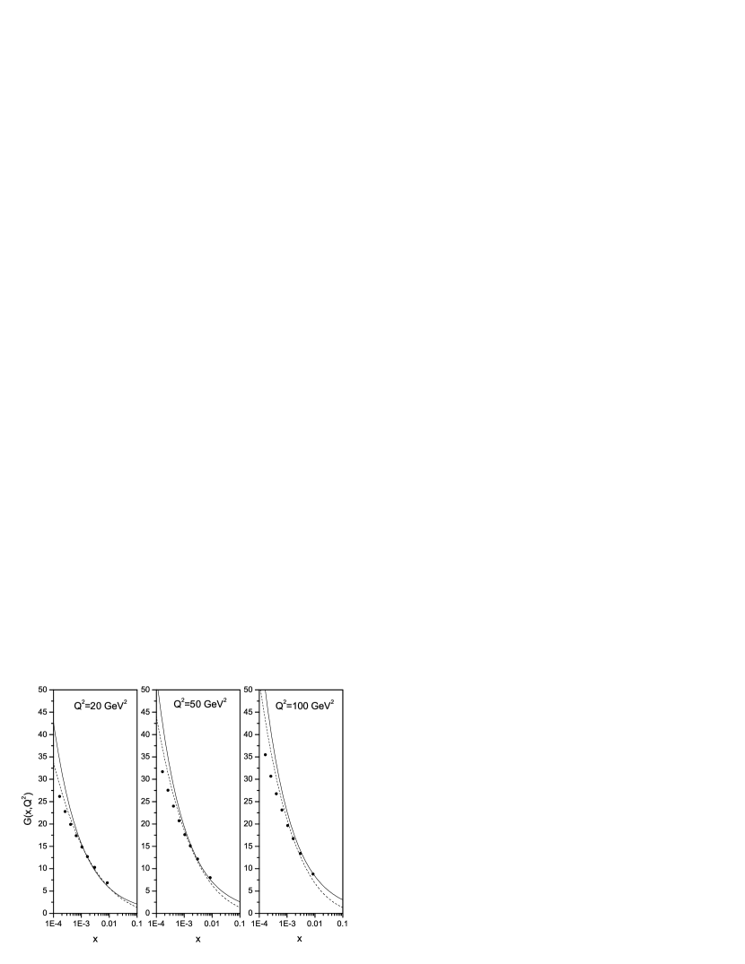
Figure 1: The gluon distribution against $x$ at fixed $Q^{2}$ values (solid circles) compared with the DL fit [7,29](solid line) and the GRV parameterization[28] (dashed line).

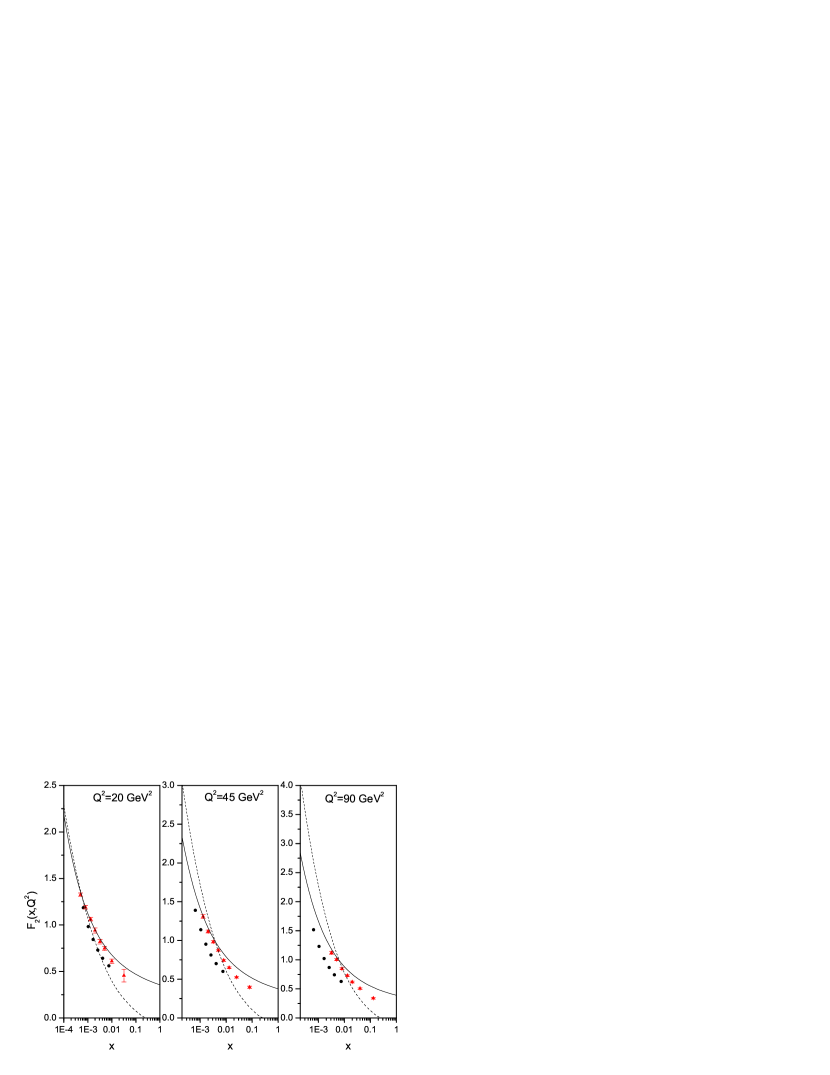
Figure 2: The calculated values of the structure function $F_{2}$ for several values of $Q^{2}$ plotted as function of $x$ with the starting parameterization of the structure function at $Q_{0}^{2}=5GeV^{2}$ (solid circles), compared with the next- to- leading order QCD fit to the H1 data with total errors (up triangle) also with the DL fit[7,29] (solid line) and dotted line represents Ref.[23] results for the GRV parameterization of the gluon distribution function to the proton structure function.