An approximate approach to the nonlinear DGLAP evaluation equation

Abstract

We determined the effects of the first nonlinear corrections to the gluon distribution using the solution of the QCD nonlinear Dokshitzer-Gribov-Lipatov-Altarelli-parisi (NLDGLAP) evolution equation at small $x$. By using a Laplace-transform technique, the behavior of the gluon distribution is obtained by solving the Gribov, Levin, Ryskin, Mueller and Qiu (GLR-MQ) evolution equation with the nonlinear shadowing term incorporated. We show that the strong rise that is corresponding to the linear QCD evolution equations at small-$x$ can be tamed by screening effects. Consequently, the nonlinear effects for the gluon distributions are calculated and compared with the results for the integrated gluon density from the Balitsky- Kovchegov(BK) equation. The resulting analytic expression allow us to predict the shadowing correction to the logarithmic derivative $F_{2}(x,Q^{2})$ with respect to ${\ln}Q^{2}$ and to compare the results with H1 data and a QCD analysis fit.

.1 1.Introduction

Perturbative QCD (PQCD) predicts a strong rise of the gluon density $xg(x,Q^{2})$ at a small value of the Bjorken variable $x$(${<<}1$), where ,as usual, $x$ denotes the momentum fraction carried by the gluon and $Q^{2}$ is the scale at which the distribution is probed. This fact that gluon density increase as $x$ decreases follows directly from linear evolution equations [1-5]. This strong rise can eventually violate unitarity and so it has to be tamed by screening effects. This behavior necessitates a chance in the evolution equation in the region of small-$x$. At small-$x$, the problem is more complicated since recombination processes between gluons in a dense system have to be taken into account, and so it has to be tamed by screening effects. These screening effects are provided by multiple gluon interaction which leads to the nonlinear terms [6-7] in the Dokshitzer- Gribov- Lipatov- Altarelli- Parisi (DGLAP) evolution equations [1-3]. These nonlinear terms reduce the growth of the gluon distribution in this kinematic region where $\alpha_{s}$ is still small but the density of partons becomes so large. Gribov, Levin, Ryskin, Mueller and Qiu (GLR-MQ)[6,8] performed a detailed study of this region. They argued that the physical processes of interaction and recombination of partons become important in the parton cascade at a large value of the parton density, and that these shadowing corrections could be expressed in a new evolution equation. This is the so-called GLR-MQ equation.
The main characteristic of this equation is that it predicts a saturation of the gluon distribution at very small-$x$ [8]. This equation was based on two processes in a parton cascade:
i)The emission induced by the QCD vertex $G{\rightarrow}G+G$ with the probability which is proportional to $\alpha_{s}\rho$ where $\rho(=\frac{xg(x,Q^{2})}{{\pi}R^{2}})$ is the density of gluon in the transverse plane, ${\pi}R^{2}$ is the target area, and $R$ is the size of the target which the gluons populate;
ii)The annihilation of a gluon by the same vertex $G+G{\rightarrow}G$ with probability which is proportional to $\frac{\alpha_{s}^{2}\rho^{2}}{Q^{2}}$, where $\alpha_{s}$ is the probability of the processes.

When $x$ is not too small, only the emission of new partons is essential because $\rho$ is small and this emission is described by the DGLAP evolution equations. Since gluon recombination introduces a negative correction to the DGLAP evolution equations, the signal of its presence is a decrease of the scaling violations as compared to the expectations obtained from the DGLAP equations. However as $x\rightarrow 0$ the value of $\rho$ becomes so large that the annihilation of partons becomes important. This picture allows us to write the GLR-MQ equation for the gluon distribution function behavior at small-$x$ [10-11]. The shadowing corrections arise from fusion of two gluon ladders, and they modify the evolution equations of gluons as

$$\frac{{\partial}xg(x,Q^{2})}{{\partial}{\ln}Q^{2}} = \frac{{\partial}xg(x,Q^{2})}{{\partial}{\ln}Q^{2}}|_{DGLAP}$$ (1)

$$-\frac{\alpha^{2}_{s}\gamma}{R^{2}Q^{2}}\int^{1}_{\chi}\frac{dy}{y}[yg(y,Q^{2})]^{2},$$

where the first term is the standard DGLAP result[1-3], linear in the parton distribution functions (PDFs) and the second term is the 2-gluon density. Thus the equation (1) becomes nonlinear in $xg$. In this equation, $\gamma$ is equal to $\frac{81}{16}$ for $N_{c}=3$. Here the representation for the gluon distribution $G(x)=xg(x)$ is used, where $g(x)$ is the gluon density and $\chi=\frac{x}{x_{0}}$, where $x_{0}(=0.01)$ is the boundary condition that the gluon distribution joints smoothly onto the unshadowed region. We neglect the quark-gluon emission diagrams due to their little importance in the gluon rich small-$x$ region and we work under an approximation of neglecting contribution from the high twist gluon distribution $G_{HT}(x,Q^{2})$ [6].
In the present paper, we extend the method using a Laplace-transform technique as proposed at Refs.[12-14]. Here we derive solution for the gluon distribution function in terms of the initial condition using the Laplace transform method, then extended this method for obtain an analytical solution of the GLR-MQ equation as the shadowing corrections to the gluon distribution functions can be determine in terms of the initial gluon distribution at $Q_{0}^{2}$.
We perform the check of our calculations by comparing the determined gluon density function with the solution of the more precise and more complicated BK equation [15-17]. Here the BK equation was derived for the deep inelastic scattering of the virtual photon on a large nucleus by the resummation of multiple Pomeron exchanges in the leading logarithmic approximation and in the large $N_{c}$ limit. It is an equation for the imaginary part of the forward scattering amplitude of the $q\overline{q}$ dipole on the nucleus. In the infinite momentum frame, the BK equation resumes fan diagrams with the BFKL [18-20] ladders, corresponding to the Pomeron, splitting into two ladders. This type of summation was originally proposed by GLR in the double logarithmic approximation (DLA) ($\alpha_{s}<<1$ and $\alpha_{s}ln(\frac{1}{x})ln(\frac{Q^{2}}{\Lambda^{2}}){\sim}1$). The non-linear evolution equation for the amplitude reduce to the GLR equation for the integrated gluon distribution. The model based on nonlinear DGLAP (NLDGLAP) shows a correspondence with the BK equation solution that calculates the values of the integrated gluon density [21-27] at the initial point.
To determine the appropriate behavior we need to specify the shadowing corrections to the gluon distribution at the initial point. The unshadowed distribution to the gluon ($g^{u}$) at $Q_{0}^{2}$ has to modifying for $x<x_{0}$ as

$$xg(x,Q^{2}_{0})=xg^{u}(x,Q^{2}_{0})[1+\theta(x_{0}-x)[xg^{u}(x,Q^{2}_{0})$$

$$-xg^{u}(x_{0},Q^{2}_{0})]/xg_{sat}(x,Q^{2}_{0})]^{-1},$$ (2)

where $xg_{sat}(x,Q^{2})=\frac{16R^{2}Q^{2}}{27\pi\alpha_{s}(Q^{2})}$ is the value of the gluon which would saturate the unitarity limit in the leading shadowing approximation. The value of $R$ is depends on how the gluon ladders couple to the proton, or on how the gluons are distributed within the proton. $R$ will be of the order of the proton radius $(R\simeq 5\hskip 2.84544ptGeV^{-1})$ if the gluons are spread throughout the entire nucleon, or much smaller $(R\simeq 2\hskip 2.84544ptGeV^{-1})$ if gluons are concentrated in hot- spot [28] within the proton. Equation (2) satisfies the requirements expected for the shadowing corrections to the gluon distribution function in $Q_{0}^{2}$. It reduces to the unshadowed form $xg^{u}$ when shadowing is negligible; that is, when $xg_{sat}{\rightarrow}\infty$. In this region, the interaction of gluons is negligible and we may continue to use evolution equations linear in $g(x,Q^{2})$. However, at sufficiently small-$x$, two gluons in different cascades may interact, generally fusion the gluon ladders together and so decrease the gluon density. Therefore shadowing contributions can no longer be neglected.

This paper is organized as follows. In Sect.2, we derive the LO master formula to extract the gluon distribution at small-$x$ from the initial condition. Section 3 is devoted to the analytical solution of the master equation for the gluon distribution functions using a Laplace-transform technique. In section 4 we consider the nonlinear corrections to the gluon distribution function with respect to the GLR-MQ equation using a Laplace method. In the last section, we calculate numerically the gluon distribution functions from the standard DGLAP and NLDGLAP evolution equation with respect to the GLR-MQ corrections, respectively. Our conclusion is given in Sect.6.

.2 2. LO master formula

The LO DGLAP equation for the evolution of the gluon distribution function at small-$x$ can be written as

$$\frac{{\partial}G(x,Q^{2})}{{\partial}{\ln}Q^{2}}|_{DGLAP}=$$

$$\frac{\alpha_{s}}{4\pi}\{G(x,Q^{2})(\frac{1}{3}(33-2n_{f})+12{\ln}(1-x))$$

$$+12x[\int_{x}^{1}G(z,Q^{2})(\frac{z}{x}-2+\frac{x}{z}-(\frac{x}{z})^{2})\frac{dz}{z^{2}}$$

$$+\int_{x}^{1}(G(z,Q^{2})-G(x,Q^{2}))\frac{z}{z-x}\frac{dz}{z^{2}}]\},$$ (3)

where $n_{f}$ being the number of active quark flavors (and $G(x,Q^{2})=xg(x,Q^{2})$). In Eq.(3), the LO $g{\rightarrow}g$ splitting functions after the convolution integral which contains plus prescription, $()_{+}$, are given by

$$K_{1}(x)=\frac{1}{x}-2+x-x^{2},$$ (4)

and

$$K_{2}(x)=\frac{1}{1-x}.$$ (5)

Note that Eq.(3) continue to hold at next-to-leading order with modified gluon splitting function. To extract the shadowing gluon distribution function, we first should be able to derive the DGLAP equation for the gluon distribution function using a Laplace-transform technique. This issue is the subject of the next section.

.3 3. Solution of the DGLAP equation for $G(x,Q^{2})$

To solve the standard DGLAP evolution equation for the gluon distribution function at small-$x$, we follow the procedure that was used by BDM [13] and employ the Laplace-transform method to solve this equation. Now we use the coordinate transformation

$$\upsilon {\equiv} \ln(1/x).$$ (6)

Then the functions $\hat{G}$, $\hat{K}$, and $\hat{\mathcal{G}}$ in $\upsilon$-space are define by

$$\hat{G}(\upsilon,Q^{2}) {\equiv} \hat{G}(e^{-\upsilon},Q^{2})$$ (7)

$$\hat{K}(\upsilon) {\equiv} \hat{K}(e^{-\upsilon})$$ (8)

$$\hat{\mathcal{G}}(\upsilon,Q^{2}) {\equiv} \frac{\alpha_{s}}{4\pi}\frac{{\partial}\hat{G}(e^{-\upsilon},Q^{2})}{{\partial}{\ln}Q^{2}}.$$ (9)

Explicitly from Eqs.(3-5), we have

$$\hat{k}(\upsilon)=\beta_{0}+12\ln(1-e^{-\upsilon}),$$ (10)

$$\hat{K_{1}}(\upsilon) = e^{\upsilon}-2+e^{-\upsilon}-e^{-2\upsilon}$$ (11)

and

$$\hat{K_{2}}(\upsilon) = \frac{1}{1-e^{-\upsilon}}.$$ (12)

In this representation, Eq.(3) reduces to this form

$$\hat{\mathcal{G}}(\upsilon,Q^{2})=\hat{G}(\upsilon,Q^{2})\hat{k}(\upsilon)$$

$$+12[\int_{0}^{\upsilon}\hat{G}(\omega,Q^{2})e^{-(\upsilon-\omega)}\hat{K}_{1}(\upsilon-\omega)$$

$$+\int_{0}^{\upsilon}(\hat{G}(\omega,Q^{2})-\hat{G}(\upsilon,Q^{2}))e^{-(\upsilon-\omega)}\hat{K}_{2}(\upsilon-\omega)],$$ (13)

or

$$\hat{\mathcal{G}}(\upsilon,Q^{2}) = \hat{G}(\upsilon,Q^{2})\hat{k}(\upsilon)+12[\int_{0}^{\upsilon}\hat{G}(\omega,Q^{2})\hat{H}_{1}(\upsilon-\omega)$$

$$+\int_{0}^{\upsilon}(\hat{G}(\omega,Q^{2})-\hat{G}(\upsilon,Q^{2}))\hat{H}_{2}(\upsilon-\omega)]$$

where

$$\hat{H}_{1}(\upsilon) {\equiv} e^{-\upsilon}\hat{K}_{1}(\upsilon)=1-2e^{-\upsilon}+e^{-2\upsilon}-e^{-3\upsilon}$$ (15)

and

$$\hat{H}_{2}(\upsilon) {\equiv} e^{-\upsilon}\hat{K}_{2}(\upsilon)=\frac{e^{-\upsilon}}{1-e^{-\upsilon}}.$$ (16)

We introduce the notation that the Laplace transformation of a function $\hat{H}(\upsilon)$ is given by $h(s)$, where

$$h(s) {\equiv} {\mathcal{L}}[\hat{H}(\upsilon);s]=\int_{0}^{\infty}\hat{H}(\upsilon)e^{-s\upsilon}d\upsilon.$$ (17)

Then Eq.(14) reduced to the form

$${\mathcal{G}}(s,Q^{2})={\mathcal{L}}[\hat{G}(\upsilon,Q^{2})\hat{k}(\upsilon);s]+12{G}(s,Q^{2}){h}_{1}(s)$$

$$+12{\mathcal{L}}[\int_{0}^{\upsilon}(\hat{G}(\omega,Q^{2})-\hat{G}(\upsilon,Q^{2}))\hat{H}_{2}(\upsilon-\omega);s],$$ (18)

where we used the following property for Laplace transformation

$${\mathcal{L}}[\int_{0}^{\upsilon}\hat{G}(\omega,Q^{2})\hat{H}(\upsilon-\omega);s]={G}(s,Q^{2}){h}(s).$$ (19)

Let us note that some sentences are very small at the limit low Bjorken scaling values, therefore we can estimate $G(s,Q^{2})$ as follow

$$\frac{{\partial}G(s,Q^{2})}{{\partial}{\ln}Q^{2}}{\simeq}\frac{\alpha_{s}}{4\pi}(\beta_{0}+12{h}_{1}(s)){G}(s,Q^{2}).$$ (20)

Integrating both part of this equation, then Eq.(20) reduced to this form

$$G(s,Q^{2})=G(s,Q_{0}^{2})\exp[(1+\frac{12}{\beta_{0}}{h}_{1}(s))\eta(Q^{2})]$$ (21)

where $\eta(Q^{2})=\int_{Q_{0}^{2}}^{Q^{2}}\frac{1}{{\ln}\frac{Q^{2}}{\Lambda^{2}}}d{\ln}Q^{2}$.
In order to find solution for $G(x,Q^{2})$, using the inverse Laplace transformation ${\mathcal{L}}^{-1}[G(s,Q^{2});\upsilon]=\hat{G}(\upsilon,Q^{2})$. Then we find that

$${\mathcal{L}}^{-1}[G(s,Q^{2});\upsilon]={\mathcal{L}}^{-1}[G(s,Q_{0}^{2})e^{[(1+\frac{12}{\beta_{0}}{h}_{1}(s))\eta(Q^{2})]};\upsilon]$$

and finally

$$\hat{G}(\upsilon,Q^{2})=e^{\eta(Q^{2})}\int_{0}^{\upsilon}\hat{G}(\omega,Q_{0}^{2})\hat{J}(\upsilon-\omega)d\omega.$$ (23)

where $\hat{J}(\upsilon)$ is defined by

$$\hat{J}(\upsilon) {\equiv} {\mathcal{L}}^{-1}[e^{\zeta{h}_{1}(s)};\upsilon].$$ (24)

and ${\zeta}{\equiv}\frac{12\eta(Q^{2})}{\beta_{0}}$.
Eq.(23) can be regarded as the equation in terms of $s$ for $e^{\zeta{h}_{1}(s)}$. In order to solve this equation we take the first term of ${h}_{1}(s)$, i.e. $\hat{J}(\upsilon)$ obtained in terms of the Dirac delta and Bessel functions of the first kind, as

$$\hat{J}(\upsilon)=\delta(\upsilon)+\frac{\sqrt{\zeta}}{\sqrt{\upsilon}}BesselI(1,2\sqrt{\zeta}\sqrt{\upsilon}),$$

and for the other terms we have

$${\mathcal{L}}^{-1}[\exp(\frac{-2\zeta}{s+1});\upsilon]=e^{-\upsilon}(\delta(\upsilon)$$

$$+\frac{\sqrt{-2\zeta}}{\sqrt{\upsilon}}BesselI(1,2\sqrt{-2\zeta}\sqrt{\upsilon})),$$ (26)

$${\mathcal{L}}^{-1}[\exp(\frac{\zeta}{s+2});\upsilon]=e^{-2\upsilon}(\delta(\upsilon)$$

$$+\frac{\sqrt{\zeta}}{\sqrt{\upsilon}}BesselI(1,2\sqrt{\zeta}\sqrt{\upsilon})),$$ (27)

$${\mathcal{L}}^{-1}[\exp(\frac{-\zeta}{s+3});\upsilon]=e^{-3\upsilon}(\delta(\upsilon)$$

$$+\frac{\sqrt{-\zeta}}{\sqrt{\upsilon}}BesselI(1,2\sqrt{-\zeta}\sqrt{\upsilon})).$$ (28)

Combining (25) with (23) and using the properties of Dirac delta function, we therefore obtain an explicit solution for the gluon distribution function in $x$ space in terms of the initial condition

$$G(x,Q^{2})=e^{\eta(Q^{2})}[G(x,Q_{0}^{2})+\int_{x}^{1}G(z,Q_{0}^{2}){\times}$$

$$\frac{\sqrt{\zeta}}{\sqrt{{\ln}\frac{z}{x}}}BesselI(1,2\sqrt{\zeta}\sqrt{{\ln}\frac{z}{x}})\frac{dz}{z}].$$ (29)

It should be noted that the size of Eqs.(26-28) are very small at low-$x$ values. Eq.(29) means that we can use the Laplace transform method for the solution of the DGLAP evolution equation at small-$x$ values as the gluon distribution is dominant at this region. This result is completely general and gives the evolution solution for the gluon distribution function once the initial gluon distribution function is known. In the next section we propose this method for determining of the shadowing corrections to the gluon distribution function with respect to the GLR-MQ equation.

.4 4. Approximate solution of the GLR-MQ equation

The GLR-MQ equation slow down the $Q^{2}$ evolution of gluons from the standard DGLAP behavior. Theses corrections arise from fusion of two gluon ladders, and they modify the evolution equations of gluons as gluons have a high density at small-$x$ according to the equation (1). The main purpose of this paper is to find an approximate solution for the non-linear DGLAP evolution equation in the saturation effects region. It is useful to consider the GLR-MQ equation in a $\upsilon$ space. In $\upsilon$ space, we have defined the Laplace transform of the $\int\frac{dy}{y}[G(y,Q^{2})]^{2}{\equiv}{\int}dw[\widehat{G}(w,Q^{2})]^{2}=\frac{1}{s}\mathcal{L}[(\widehat{G}(\upsilon,Q^{2}))^{2};s]$ to be less than $\frac{1}{s}[G(s,Q^{2})]^{2}$. Therefore in this limit, we take the Laplace transform of (1), by follow

$$\frac{{\partial}G(s,Q^{2})}{{\partial}{\ln}Q^{2}} {\simeq} \frac{{\partial}G(s,Q^{2})}{{\partial}{\ln}Q^{2}}|_{DGLAP}$$ (30)

$$-\frac{81\alpha^{2}_{s}}{16R^{2}Q^{2}}\frac{1}{s}[G(s,Q^{2})]^{2},$$

According to Eq.(20), we rewrite Eq.(30) in terms of the gluon transformed in $s$-space

$$\frac{{\partial}G(s,Q^{2})}{{\partial}{\ln}Q^{2}} = {\psi}G(s,Q^{2})-{\varphi}G^{2}(s,Q^{2}),$$ (31)

where $\psi=(1+\frac{12h_{1}(s)}{\beta_{0}})\frac{1}{{\ln}\frac{Q^{2}}{\Lambda^{2}}}$ and $\varphi=\frac{81\pi^{2}}{s\beta^{2}_{0}R^{2}Q^{2}(\ln\frac{Q^{2}}{\Lambda^{2}})^{2}}$. One may write the solution in fact directly in terms of the initial condition, as

$$G(s,Q^{2}) = G(s,Q_{0}^{2})e^{\int_{Q_{0}^{2}}^{Q^{2}}{\psi}d{\ln}Q^{2}}$$

$${\times}[1+G(s,Q_{0}^{2})\int_{Q_{0}^{2}}^{Q^{2}}e^{\int{\psi}d{\ln}Q^{2}}{\varphi}d{\ln}Q^{2}]^{-1}.$$

Further, we can rewrite Eq.(32) by

$$G(s,Q^{2}) = G(s,Q_{0}^{2})e^{\int_{Q_{0}^{2}}^{Q^{2}}{\psi}d{\ln}Q^{2}}-G^{2}(s,Q_{0}^{2})e^{\int_{Q_{0}^{2}}^{Q^{2}}{\psi}d{\ln}Q^{2}}$$

$${\times}\int_{Q_{0}^{2}}^{Q^{2}}e^{\int{\psi}d{\ln}Q^{2}}{\varphi}d{\ln}Q^{2}+{\mathcal{O}}(2)-{\mathcal{O}}(3)+...$$

We will generally be able to calculate the inverse Laplace transform of $G(s,Q^{2})$ explicitly and transforming back into $x$ space. Finally the shadowing corrections to the gluon distribution function $G(x,Q^{2})$ obtained in terms of the initial function $G(x,Q_{0}^{2})$, assumed to be known, by

$$G(x,Q^{2}) = [Eq.29]-\int_{\chi}^{1}G^{2}(z,Q_{0}^{2})Fe^{Y}$$ (34)

$${\times}BesselI(0,2\sqrt{U}\sqrt{{\ln}\frac{z}{x}})\frac{dz}{z}$$

$$+{\mathcal{O}}(2)-{\mathcal{O}}(3)+...$$

In the above equation, the Bessel functions obtained from the property for inverse Laplace transformation

$${\mathcal{L}}^{-1}[\frac{F}{s}e^{Y}e^{\frac{U}{s}};\upsilon]=Fe^{Y}BesselI(0,2\sqrt{U}\sqrt{\upsilon})),$$ (35)

where the functions $F,U$ and $Y$ obtained from the below equation after integration and some rearranging

$$Fe^{Y}e^{\frac{U}{s}} {\equiv} e^{\int^{Q^{2}}_{Q_{0}^{2}}{\psi}d{\ln}Q^{2}}\int^{Q^{2}}_{Q_{0}^{2}}e^{(1+\frac{12h_{1}(s)}{\beta_{0}}){\ln}{\ln}\frac{Q^{2}}{\Lambda^{2}}}{\varphi}d{\ln}Q^{2}.$$

This method can be used for order ${\mathcal{O}}(2)$ and other orders, as they are very small at low-$x$. This solution in the form of Eq.(34) has a very clear physical meaning. We expect that gluon correlations in the parton cascade at the region of the small-$x$ tamed the behavior of the gluon distribution function. Therefore we observed that the terms add to Eq.(29) on r.h.s of Eq.(34) are due to the saturation effects.

.5 5.Numerical Estimates

In this paper, we found two analytical solutions for the standard DGLAP and NLDGLAP evolution equations for the gluon distribution function inside the proton. These equations (Eqs.29 and 34) are directly related to the initial conditions and they are independent of the gluon behavior at small-$x$. We determined the unshadowing and shadowing corrections to the gluon distribution functions using a Laplace-transform method in Eqs.29 and 34, respectively. Despite the analytical calculations that led us to the solutions in the forms of Eqs.(29) and (34), we will solved these equations numerically. In these calculations, we use the LO form of $\alpha_{s}(Q^{2})$ which is defined by

$$\alpha_{s}(Q^{2}) {\equiv} \frac{12\pi}{25\ln(\frac{Q^{2}}{\Lambda^{2}})},$$ (37)

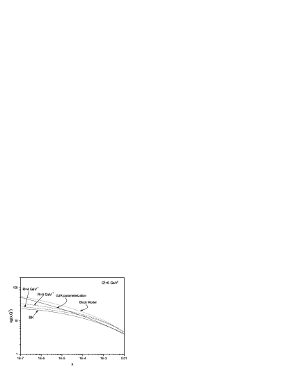
for four active flavors, where $\Lambda$ is the QCD cut- off parameter. The input gluon parameterization can be taken from the BDM model [12] at the starting scale $Q_{0}^{2}=5~{}\mathrm{GeV}^{2}$. In Fig.1, we show shadowing corrections to the gluon distribution function determined from Eq.(2) as a function of $x$ at the initial scale $Q_{0}^{2}$ based on the size of the target which the gluons populate. We observed that, as $x$ decreases, the singularity behavior of the gluon functions are tamed by shadowing effects. The top curves (solid and dot) show the small-$x$ behavior of the gluon distribution when shadowing is neglected, and the lower curves (dash) show the effect of the shadowing contribution for $R=5$ and $4~{}GeV^{-1}$. We compared our results with BK [15-17](dash-dot) curve and GJR parameterization [29] (solid).
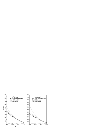
In Fig.2, we show the unshadowed corrections to the gluon distribution function $G(x,Q^{2})$ determined from Eq.(29) as a function of $x$ for two different values of $Q^{2}$, namely $Q^{2}=20$ and $Q^{2}=50~{}GeV^{2}$ with respect to the Laplace-transform method. We compared our results with GJR parameterization [29] and BDM model [12]. By using this method, we show that our results are general and independent of the gluon behavior at small-$x$. As can be seen, the values of the gluon distribution increase as $x$ decreases.
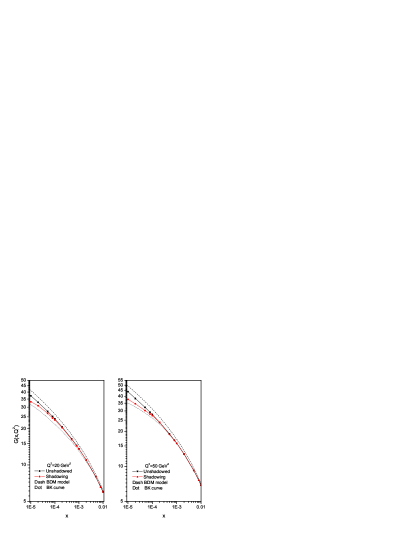
In Fig.3, we show the shadowing corrections to the gluon distribution function determined from Eq.(34). To evaluate the NLDGLAP equation, by using a Laplace-transform method, we have generalized the BDM [12-13] approach from linear to nonlinear case at small-$x$. The results are shown for $Q^{2}=20$ and $Q^{2}=50~{}GeV^{2}$. The top curve (squared) shows the small-$x$ behavior of the gluon distribution when shadowing is neglected, and the lower curve (circled) shows the effects of the shadowing corrections at the extreme ”hot- spot” point [30] with $R=2\hskip 2.84544ptGeV^{-1}$. Our results compared with the integrated gluon density function, which is denote as BK curve. These results show that gluon density behavior increase as x decreases, this corresponds with PQCD fits at low-$x$, but this behavior is tamed with respect to nonlinear terms at the GLR-MQ equation. This figure compares the results of two calculations, based on the linear and nonlinear equations. The differences are not large, however there is some suppression due to the nonlinearity at smallest values of $x{\leq}10^{-4}$. It is clear that a new evolution equation for the gluon density relevant for the region of small-$x$. It show that screening effects are provided by multiple gluon interaction which leads to the nonlinear terms in the DGLAP equation.
In order to compare our results with the experimental data, we follow the role of shadowing correction to the evolution of the singlet quark distribution with respect to GLR-MQ equations. Indeed, the DGLAP evolution equation of the $Q^{2}$ logarithmic slope of $F_{2}$ at low $x$, at leading order, is directly proportional to the gluon structure function. But, according to these corrections (fusion of two gluon ladders), the shadowing corrections to the evolution of the structure function with respect to ${\ln}Q^{2}$ corresponds with a modified DGLAP evolution equation [10-11,30-32]. At low $x$, the nonsinglet contribution is negligible and can be ignord, so that

$$\frac{{\partial}F_{2}(x,Q^{2})}{{\partial}{\ln}Q^{2}} = \frac{{\partial}F_{2}(x,Q^{2})}{{\partial}{\ln}Q^{2}}|_{DGLAP}$$ (38)

$$-\frac{5}{18}\frac{27\alpha_{s}^{2}}{160R^{2}Q^{2}}[xg(x,Q^{2})]^{2},$$

where the first term is the standard DGLAP evolution equation.
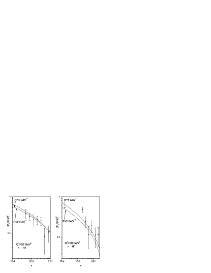
To find an analytical solution for the shadowing corrections to the derivative of $F_{2}$ at low $x$, we intend to use the gluon functions obtained in Eq.38. We show a plot of $\frac{{\partial}F_{2}(x,Q^{2})}{{\partial}{\ln}Q^{2}}$ in Fig.4 for a the values of $Q^{2}=20GeV^{2}$ and $50GeV^{2}$ at the points $R=2GeV^{-1}$ and $4GeV^{-1}$, compared to the values measured by the H1 collaboration [33-34] and a QCD fit based on ZEUS data [35]. From this figure one can see the GLR-MQ equation is tamed behavior with respect to gluon saturation as $Q^{2}$ increases. Consequently, derivative of the shadowing corrections to the structure function with respect to ${\ln}Q^{2}$ at fixed $x$ is close to H1 data and to the QCD analysis fit. This shadowing correction suppresses the rate of growth in comparison with the DGLAP approach.

.6 6.Conclusions

In this paper, we studied the effects of adding the nonlinear GLR-MQ corrections to the LO DGLAP evolution equation, by using a Laplace-transform method suggested by the BDM [12-14], in order to determine the small-$x$ behavior of the gluon distribution $xg(x,Q^{2})$ of the proton. In this way we were able to study the interplay of the singularity behavior, generated by the linear term of the equation, with the taming of this behavior by the nonlinear shadowing term. The nonlinear effects to the gluon distribution are found to play an increasingly important at $x{\leq}10^{-4}$. The nonlinearities, however, vanish rapidly at large values of $x$. We observed that, as $x$ decreases, the singularity behavior of the gluon function is tamed by shadowing effects. Our results compared with the gluon distribution obtained in a QCD analysis and with the BK equation. The obtained results are comparable with the results obtained by basing on the BK equation. Based on our present calculations we conclude that the behavior of $\frac{{\partial}F_{2}(x,Q^{2})}{{\partial}{\ln}Q^{2}}$ as measured at HERA, tamed based on gluon saturation at low $x$. The expansion of the results from LO to NLO approximation can be done as a new research job in future.

I References

1.Yu.L.Dokshitzer, Sov.Phys.JETP 46, 641(1977).
2.G.Altarelli and G.Parisi, Nucl.Phys.B 126, 298(1977).
3.V.N.Gribov and L.N.Lipatov, Sov.J.Nucl.Phys. 15, 438(1972).
4. A.De Rujula et al., phys.Rev.D 10, 1649(1974).
5. R.D.Ball and S.Forte, Phys.Lett.B 335, 77(1994).
6. A.H.Mueller and J.Qiu, Nucl.Phys.B268, 427(1986).
7. J.Kwiecinski and A.M.Stasto, Phys.Rev.D66, 014013(2002).
8. L.V.Gribov, E.M.Levin and M.G.Ryskin, Phys.Rep.100, 1(1983).
9. A.L.A.Filho. M.B.Gay Ducati and V.P.Goncalves, Phys.Rev.D59,054010(1999).
10. E.Laenen and E.Levin,Nucl.Phs.B.451,207(1995).
11. K.J.Eskola, et.al., Nucl.Phys.B660, 211(2003).
12.M.M.Block, L.Durand, D.W.McKay, Phys.Rev.D77, 094003(2008).
13.M.M.Block, L.Durand, D.W.McKay, Phys.Rev.D79, 014031(2009).
14.M.M.Block, Eur.Phys.J.C65, 1(2010).
15. I.I.Balitsky, Nucl.Phys.B463, 99(1996).
16.Yu.V.Kovchegov, Phys.Rev.D60, 034008(1999).
17.Yu.V.Kovchegov, Phys.Rev.D61, 074018(2000).
18. E.A.Kuraev, L.N.Lipatov and V.S.Fadin, Sov.Phys.JETP 44, 443(1976).
19. E.A.Kuraev, L.N.Lipatov and V.S.Fadin, Sov.Phys.JETP 45, 199(1977).
20. Y.Y.Balitsky and L.N.Lipatov, Sov.Journ.Nucl.Phys. 28, 822(1978).
21. K.Golec-Biernat, L.Motyka, and A.M.Stasto, Phys.Rev.D65, 074037(2002).
22. J. Kwiecinski, A.D. Martin, P.J. Sutton, Phys. Rev. D 44, 2640 (1991).
23. A.J. Askew, J. Kwiecinski, A.D. Martin, P.J. Sutton, Phys.Rev. D 47, 3775 (1993).
24. S.Bondarenko, Phys.Lett.B665, 72(2008).
25. K.Kutak and A.M.Stasto, Eur.Phys.J.C41, 343(2005).
26. M.Kazlov and E.Levin, Nucl.Phys. A764, 498 (2006).
27. M.A.Kimber, J.Kwiecinski and A.D.Martin, Phys.Lett. B508, 58(2001).
28.E.M.Levin and M.G.Ryskin, Phys.Rep.189, 267(1990).
29.M. Gluck, P. Jimenez-Delgado, E. Reya, Eur.Phys.J.C 53,355 (2008).
30. A.H. Mueller,arXiv:hep-ph/0111244(2001).
31. E.Gotsman,et.al., Nucl.Phys.B539, 535(1999).
32. E.Gotsman,et.al., Phys.Lett.B500, 87(2001).
33. $H1$ Collab., C.Adloff et al., Eur.Phys.J.C 13, 609(2000). 34. $H1$ Collab., C.Adloff et al., Eur.Phys.J.C 21, 33(2001).
35. E.L.Berger, M.M.Block and C.I Tan, Phys.Rev.Lett98, 242001(2007).

Figure 1: The shadowing corrections to the gluon distribution function at $Q_{0}^{2}=5\hskip 2.84544ptGeV^{2}$ from the solution of the initial condition shadowing effects based on Eq.2 with the boundary condition at $x_{0}=10^{-2}$. The dot curve is the BDM model [12] with unshadowed corrections and dash curves are our results with the shadowing corrections included with $R=4\hskip 2.84544ptGeV^{-1}$ and $R=5\hskip 2.84544ptGeV^{-1}$ that compared with BK [15-17,24-27] integrated gluon density function (dash-dot) and GJR [29] parameterization (solid) at small-$x$.

Figure 2: Unshadowed LO gluon distribution function at $Q^{2}=20$ and $50~{}GeV^{2}$ according to the gluon distribution input [12] compared with results BDM model [12] and GJR [29] parameterization at small-$x$.

Figure 3: Shadowing corrections to the gluon distribution function included with $R=2\hskip 2.84544ptGeV^{-1}$ at $Q^{2}=20$ and $50~{}GeV^{2}$ compared with results BDM model [12] and BK [15-17,24-27] equation at small-$x$ .

Figure 4: A plot of the derivative of the shadowing corrections to the structure function with respect to ${\ln}Q^{2}$ for $Q^{2}=20GeV^{2}$ and $50GeV^{2}$ at the points $R=2GeV^{-1}$ (Dot-line)and $4GeV^{-1}$ (Dash-line), compared to data from H1 Collab.[33-34] (circles) with total error, and also a QCD fit to ZEUS data [3](solid-line).