Complete Tidal Evolution of Pluto-Charon

Abstract

Both Pluto and its satellite Charon have rotation rates synchronous with their orbital mean motion. This is the theoretical end point of tidal evolution where transfer of angular momentum has ceased. Here we follow Pluto’s tidal evolution from an initial state having the current total angular momentum of the system but with Charon in an eccentric orbit with semimajor axis $a\approx 4R_{\scriptscriptstyle P}$ (where $R_{\scriptscriptstyle P}$ is the radius of Pluto), consistent with its impact origin. Two tidal models are used, where the tidal dissipation function $Q\propto$ 1/frequency and $Q=$ constant, where details of the evolution are strongly model dependent. The inclusion of the gravitational harmonic coefficient $C_{22}$ of both bodies in the analysis allows smooth, self consistent evolution to the dual synchronous state, whereas its omission frustrates successful evolution in some cases. The zonal harmonic $J_{2}$ can also be included, but does not cause a significant effect on the overall evolution. The ratio of dissipation in Charon to that in Pluto controls the behavior of the orbital eccentricity, where a judicious choice leads to a nearly constant eccentricity until the final approach to dual synchronous rotation. The tidal models are complete in the sense that every nuance of tidal evolution is realized while conserving total angular momentum — including temporary capture into spin-orbit resonances as Charon’s spin decreases and damped librations about the same.

1 INTRODUCTION

Pluto has five known satellites: Charon, Nix, Hydra, Keberos, and Styx, with the latter four much smaller than Charon. Listed in Table 1 are the physical and orbital parameters of Pluto-Charon from Buie et al. (2012), unless otherwise specified. The Charon-Pluto mass ratio ($q=0.1165$) is large when compared with others in the Solar System ($1/81$ for Moon-Earth and $<1/4000$ for the other satellites and their planets). The barycenter of the Pluto-Charon system lies outside the surface of Pluto. Hence, some astronomers regard the pair as a binary system (Stern, 1992). The total angular momentum $L$ of the Pluto-Charon system is so large that the combined pair would be rotationally unstable (Mignard, 1981a; Lin, 1981).

The Pluto-Charon system is currently in a dual synchronous state (Buie et al., 1997, 2010), which is the endpoint of tidal evolution. As such the expected zero orbital eccentricity has been recently verified (with a 1-$\sigma$ upper limit of $7.5\times 10^{-5}$), after taking into account the effects of surface albedo variations on Pluto (Buie et al. 2012; see Table 1).

Table 1: Physical and orbital parameters of the Pluto-Charon system

Parameter	Pluto	Charon
$GM$ (km3 s-2)	870.3(3.7)	101.4(2.8)
Radius $R$ (km)	1153(10)	606.0(1.5)
Orbital period $P$ (days)	6.3872273(3)
Semimajor axis $a$ (km)	19573(2)
Eccentricity $e$	0
Inclination $i$ (∘)	96.218(8)
Long. ascending node $\Omega$ (∘)	223.0232(69)

Note. — The orbital elements are Pluto-centric with respect to the mean equator and equinox of J2000 at the epoch JD 2452600.5. Numbers in parentheses are 1-$\sigma$ errors in the least significant digits.

As Pluto-Charon is similar to Earth-Moon, the feasible origin of this system may be chosen from the proposed schemes for the origin of the Earth-Moon system. A giant impact of a Mars-sized body is thought to be the only viable origin of the Moon (e.g., Cameron and Ward 1976; Boss and Peale 1986; Canup 2004) to account for the large angular momentum of the system. McKinnon (1984) proposed a similar origin for Charon. If Charon accumulated from a debris disk resulting from such an impact, the initial eccentricity of Charon’s orbit would be near zero. Dobrovolskis et al. (1997, hereafter DPH97) were thereby motivated to determine the tidal evolution of Charon in a circular orbit to the current dual synchronous state in a time short compared to the age of the Solar System (see also Farinella et al. 1979) as the only possible outcome of the dissipative process. In a circular orbit, Charon would reach synchronous rotation very quickly (e.g., DPH97), and this has generally been assumed (e.g., Peale 1999). However, smoothed particle hydrodynamic (SPH) simulations by Canup (2005) showed that the results of a nearly intact capture in a glancing encounter surround the $(q,L)$ region of the system much more completely than those of disk-forming impacts. Therefore, capture where Charon comes off nearly intact after a glancing impact is favored and non-zero eccentricity would be more probable.

We are not aware of any previous attempts to examine the tidal evolution of Charon’s orbit incorporating finite eccentricity. As we shall see, Charon in an initially eccentric orbit avoids the almost immediate synchronous rotation heretofore assumed, and the varied and interesting evolutionary sequences that were suppressed in the circular orbit evolution are revealed. Depending on the ratios of rigidity $\mu$ and tidal dissipation function $Q$ between Pluto and Charon, the eccentricity of Charon’s orbit may either grow or decay during most of the evolution (Ward and Canup, 2006). Permanent quadrupole moments of the bodies may also lead to spin-orbit resonance, and such resonances can have a significant effect on the orbital evolution.

In the following we tidally evolve the Pluto-Charon system with two tidal models distinguished by the dependence of the dissipation function $Q$ on frequency $f$: $Q\propto 1/f$ and $Q=$ constant. The tidal model developed in Section 2.1 has the tidal distortion of a body responding to the perturbing body a short time $\Delta t$ in the past. Constant $\Delta t$ leads to $Q\propto 1/f$, so we call the $Q\propto 1/f$ model the constant $\Delta t$ model. In Section 2.2 we develop the equations of evolution for the constant $Q$ model. Although neither of these frequency dependences represent the behavior of real solid materials (e.g., Castillo-Rogez et al. 2011) and although the evolutionary tracks are model dependent, most if not all of the possible routes from probable initial configurations to the current equilibrium state are demonstrated. In Section 2.3 we develop the contributions of rotational flattening $J_{2}$ and permanent quadrupole moment $C_{22}$ to the equations of motion. We describe the adopted system parameters and initial conditions in Section 3 and the numerical methods in Section 4. The results from both the constant $\Delta t$ and constant $Q$ models with zero $J_{2{\scriptscriptstyle P}}$ for Pluto and zero $C_{22}$ for both bodies are shown in Section 5.1, and the effects of non-zero $J_{2P}$ and $C_{22}$ in Section 5.2, respectively. The results are discussed in Section 6, and the conclusions are summarized in Section 7.

2 TIDAL MODELS

Tides are raised on Pluto and Charon by each other. Friction delays the response of the tidal bulge to the tide raising potential and causes tidal lag. The lagged bulge leads to angular momentum exchange between itself and the tide raising body, which leads to rotational and orbital evolution.

2.1 Constant $\Delta t$ Tidal Model

The idea of approximating tidal evolution with a single bulge that lags by a constant $\Delta t$ was introduced by Gerstenkorn (1955), and developed and used by Singer (1968), Alexander (1973), Mignard (1979, 1980, 1981b), Hut (1981), and Peale (2005, 2007). The advantage of assuming a single, lagged bulge is that the tidal forces and torques can be calculated in closed form for arbitrary eccentricity and inclination. Either instantaneous or orbit-averaged tidal forces and torques can be used to determine the evolution.

The geometry is illustrated in Fig. 1, where $\psi_{\scriptscriptstyle P}$ and $\psi_{\scriptscriptstyle C}$ are the angular displacements of the axes of minimum moment of inertia from the inertial $x$ axis for Pluto and Charon, respectively, $\varpi$ is the longitude of periapse, $f$ is the true anomaly, and $\phi_{\scriptscriptstyle P}$ and $\phi_{\scriptscriptstyle C}$ are the azimuthal spherical coordinates appearing in the potentials for Pluto and Charon, respectively. The $x$ and $y$ coordinates are those of Charon relative to Pluto with the $x$-$y$ plane being the Pluto-Charon orbit plane. Both spin axes are assumed to be perpendicular to the orbit plane (see Section 3). The motion is thereby two dimensional, and the $z$ coordinate is ignorable.

Figure 1: Geometry of the Pluto-Charon system with orbit and equator planes being coplanar. $\psi_{i}$ are the angles between the axes of minimum moment of inertia and the inertial $x$ axis, and the $\phi_{i}$ are the azimuthal angles locating respectively $M_{\scriptscriptstyle P}$ and $M_{\scriptscriptstyle C}$ in the other’s $x^{\scriptscriptstyle\prime}$-$y^{\scriptscriptstyle\prime}$ plane measured counterclockwise from the $x_{i}^{\scriptscriptstyle\prime}$ axes of minimum moment of inertia.

The tidal contributions to the equations of motion for Charon for this model are found from the gradient of the tidal potential expanded to first order in $\Delta t$ (Mignard, 1980; Peale, 2007):

$$M_{\scriptscriptstyle PC}\ddot{x} = -{3k_{2{\scriptscriptstyle P}}GM_{\scriptscriptstyle C}^{2}R_{\scriptscriptstyle P}^{5}\over r^{8}}\left[x+\frac{2{\bf r}\cdot\dot{\bf r}x\Delta t_{\scriptscriptstyle P}}{r^{2}}+(\dot{\psi}_{\scriptscriptstyle P}y+\dot{x})\Delta t_{\scriptscriptstyle P}\right]$$

$$-{3k_{2{\scriptscriptstyle C}}GM_{\scriptscriptstyle P}^{2}R_{\scriptscriptstyle C}^{5}\over r^{8}}\left[x+\frac{2{\bf r}\cdot\dot{\bf r}x\Delta t_{\scriptscriptstyle C}}{r^{2}}+(\dot{\psi}_{\scriptscriptstyle C}y+\dot{x})\Delta t_{\scriptscriptstyle C}\right],$$

$$M_{\scriptscriptstyle PC}\ddot{y} = -{3k_{2{\scriptscriptstyle P}}GM_{\scriptscriptstyle C}^{2}R_{\scriptscriptstyle P}^{5}\over r^{8}}\left[y+\frac{2{\bf r}\cdot\dot{\bf r}y\Delta t_{\scriptscriptstyle P}}{r^{2}}+(-\dot{\psi}_{\scriptscriptstyle P}x+\dot{y})\Delta t_{\scriptscriptstyle P}\right]$$ (1)

$$-{3k_{2{\scriptscriptstyle C}}GM_{\scriptscriptstyle P}^{2}R_{\scriptscriptstyle C}^{5}\over r^{8}}\left[y+\frac{2{\bf r}\cdot\dot{\bf r}y\Delta t_{\scriptscriptstyle C}}{r^{2}}+(-\dot{\psi}_{\scriptscriptstyle C}x+\dot{y})\Delta t_{\scriptscriptstyle C}\right],$$

where $G$ is the gravitational constant, ${\bf r}$ and $\dot{\bf r}$ are the position and velocity of Charon relative to Pluto, $M_{i}$, $R_{i}$, $\dot{\psi}_{i}$, and $k_{2i}$ are the mass, radius, spin angular velocity, and second order potential Love number, respectively, of body $i$ ($=P$ for Pluto and $=C$ for Charon), and $M_{\scriptscriptstyle PC}=M_{\scriptscriptstyle P}M_{\scriptscriptstyle C}/(M_{\scriptscriptstyle P}+M_{\scriptscriptstyle C})$ is the reduced mass. The first term on the right hand side of the first (second) equation in Eq. (1) is the $x$-component ($y$-component) of the force due to the tides raised on Pluto by Charon, and the second term is the force due to the tides raised on Charon by Pluto. The equations of motion for the spins are found from the negative of the torques on the bodies determined from the tidal forces:

$$\mathcal{C}_{\scriptscriptstyle P}\ddot{\psi}_{\scriptscriptstyle P} = -{3k_{2{\scriptscriptstyle P}}GM_{\scriptscriptstyle C}^{2}R_{\scriptscriptstyle P}^{5}\Delta t_{\scriptscriptstyle P}\over r^{6}}\left[\dot{\psi}_{\scriptscriptstyle P}+\frac{-\dot{y}x+y\dot{x}}{r^{2}}\right],$$

$$\mathcal{C}_{\scriptscriptstyle C}\ddot{\psi}_{\scriptscriptstyle C} = -{3k_{2{\scriptscriptstyle C}}GM_{\scriptscriptstyle P}^{2}R_{\scriptscriptstyle C}^{5}\Delta t_{\scriptscriptstyle C}\over r^{6}}\left[\dot{\psi}_{\scriptscriptstyle C}+\frac{-\dot{y}x+y\dot{x}}{r^{2}}\right],$$ (2)

where $\mathcal{C}_{i}$ is the moment of inertia of body $i$ about its spin axis.

Eqs. (1) and (2) can be used directly in numerical integration of the equations of motion in Cartesian coordinates. Alternatively, one can average the tidal forces and torques over an orbit to obtain the orbit-averaged equations for the variation of the spin rate $\dot{\psi}_{i}$, orbital semimajor axis $a$, and eccentricity $e$ (Mignard, 1980, 1981b):

$$\frac{1}{n}\left\langle\frac{d\dot{\psi}_{i}}{dt}\right\rangle = -\frac{3G}{C_{i}a^{6}}k_{2i}\Delta t_{i}M_{j}^{2}R_{i}^{5}\left[f_{1}(e)\frac{\dot{\psi}_{i}}{n}-f_{2}(e)\right],$$ (3)

$$\frac{1}{a}\left\langle\frac{da}{dt}\right\rangle = \frac{6G}{M_{\scriptscriptstyle PC}a^{8}}k_{2{\scriptscriptstyle P}}\Delta t_{\scriptscriptstyle P}M_{\scriptscriptstyle C}^{2}R_{\scriptscriptstyle P}^{5}\left[f_{2}(e)\left(\frac{\dot{\psi}_{\scriptscriptstyle P}}{n}+A_{\Delta t}\frac{\dot{\psi}_{\scriptscriptstyle C}}{n}\right)-f_{3}(e)(1+A_{\Delta t})\right],$$ (4)

$$\frac{1}{e}\left\langle\frac{de}{dt}\right\rangle = \frac{27G}{M_{PC}a^{8}}k_{2P}\Delta t_{\scriptscriptstyle P}M_{\scriptscriptstyle C}^{2}R_{\scriptscriptstyle P}^{5}\left[f_{4}(e)\frac{11}{18}\left(\frac{\dot{\psi}_{\scriptscriptstyle P}}{n}+A_{\Delta t}\frac{\dot{\psi}_{\scriptscriptstyle C}}{n}\right)-f_{5}(e)(1+A_{\Delta t})\right],$$ (5)

where the subscript $j=$ Charon if $i=$ Pluto, and vice versa, $\langle\ \rangle$ denotes averaging over an orbit, $n=[G(M_{\scriptscriptstyle P}+M_{\scriptscriptstyle C})/a^{3}]^{1/2}$ is the mean motion, and

$$f_{1}(e) = \left(1+3e^{2}+\frac{3}{8}e^{4}\right)\left/(1-e^{2})^{9/2}\right.,$$

$$f_{2}(e) = \left(1+\frac{15}{2}e^{2}+\frac{45}{8}e^{4}+\frac{5}{16}e^{6}\right)\left/(1-e^{2})^{6}\right.,$$

$$f_{3}(e) = \left(1+\frac{31}{2}e^{2}+\frac{255}{8}e^{4}+\frac{185}{16}e^{6}+\frac{25}{64}e^{8}\right)\left/(1-e^{2})^{15/2}\right.,$$ (6)

$$f_{4}(e) = \left(1+\frac{3}{2}e^{2}+\frac{1}{8}e^{4}\right)\left/(1-e^{2})^{5}\right.,$$

$$f_{5}(e) = \left(1+\frac{15}{4}e^{2}+\frac{15}{8}e^{4}+\frac{5}{64}e^{6}\right)\left/(1-e^{2})^{13/2}\right..$$

In Eqs. (4) and (5),

$$A_{\Delta t}=\frac{k_{2C}}{k_{2P}}\frac{\Delta t_{\scriptscriptstyle C}}{\Delta t_{\scriptscriptstyle P}}\left(\frac{M_{\scriptscriptstyle P}}{M_{\scriptscriptstyle C}}\right)^{2}\left(\frac{R_{\scriptscriptstyle C}}{R_{\scriptscriptstyle P}}\right)^{5}$$ (7)

is a measure of the relative rate of tidal dissipation in Charon and Pluto, and the same as $A$ defined in Mignard (1980) and in Eq. (13) of Touma and Wisdom (1998). $A$ depends on the tidal model and we add subscripts to distinguish them whenever necessary.

The Love number $k_{2}$ measures the elastic distortion of the body in response to the second order spherical harmonic of the deforming potential. It can be modeled as (Eq. [5.6.2] of Munk and MacDonald 1960; Eq. [40a] of Peale 1973)

$$k_{2}=\frac{k_{f}}{1+\tilde{\mu}},$$ (8)

where $k_{f}$ is the fluid Love number and $\tilde{\mu}$ is the effective rigidity. The fluid Love number $k_{f}=3/2$ for homogeneous sphere and its reduction due to differentiation is sometimes ignored (e.g., DPH97). The effective rigidity $\tilde{\mu}$ is a dimensionless quantity, and

$$\tilde{\mu}=\frac{19\mu}{2\rho gR}$$ (9)

for an incompressible homogeneous sphere of radius $R$, rigidity $\mu$, density $\rho$, and surface gravity $g$ (Eq. [5.6.1] of Munk and MacDonald 1960; Eq. [4.77] of Murray and Dermott 1999). For small solid body, $\tilde{\mu}\gg 1$ and the approximation

$$k_{2}\approx\frac{3\rho gR}{19\mu}$$ (10)

is commonly used (e.g., Peale and Cassen, 1978; Yoder and Peale, 1981; Peale, 1999, 2007). Then

$$A_{\Delta t}\approx\frac{\mu_{\scriptscriptstyle P}}{\mu_{\scriptscriptstyle C}}\frac{\Delta t_{\scriptscriptstyle C}}{\Delta t_{\scriptscriptstyle P}}\frac{R_{\scriptscriptstyle C}}{R_{\scriptscriptstyle P}}.$$ (11)

For non-zero eccentricity, the orbit-averaged tidal torque vanishes at a value of $\dot{\psi}_{i}>n$, and $\dot{\psi}_{i}$ goes to an asymptotic spin rate that increases with eccentricity. This asymptotic spin is often called a “pseudo-synchronous” state. The case for Mercury was illustrated by the curve $\delta\sim$ frequency in Fig. 1 of Goldreich and Peale (1966). Pseudo-synchronous spin rate can be obtained by setting $\langle d\dot{\psi}_{i}/dt\rangle=0$ in Eq. (3):

$$\frac{\dot{\psi}_{\rm ps}}{n}=\frac{f_{2}(e)}{f_{1}(e)}=1+6e^{2}+\frac{3}{8}e^{4}+\frac{173}{8}e^{6}+O(e^{8}).$$ (12)

For the orbit-averaged equations, we ignore the periapse motion due to the tidal bulges, as it will be small initially compared to that caused by the rotational distortion of Pluto (see Section 3). Apsidal motion does not affect our discussion as far as the tidal evolution of Pluto-Charon is concerned, but it does play an important role in the study of the hypothesis that the small satellites, Nix, Hydra, Keberos, and Styx, were brought to their current orbits by mean-motion resonances with Charon (Cheng, Lee and Peale, in preparation; hereafter paper II).

2.2 Constant $Q$ Tidal Model

A number of authors (e.g., Goldreich 1966; Goldreich and Peale 1966; Yoder and Peale 1981) have developed and applied a tidal model with a constant $Q$, based on the work of Kaula (1964). This approach has been used by the previous studies of Pluto-Charon (Farinella et al., 1979; DPH97; Ward and Canup 2006). To develop the equations of evolution for the constant $Q$ model, expansions in the orbital elements are necessary, and the orbit-averaged effect on the orbit can be derived from the Gauss planetary equations. The truncation of the expansion means the equations are no longer exact and angular momentum is no longer strictly conserved.

The tidal potential acting on one of the bodies can be written as a sum of periodic terms. The frequency of the $(l,m)$ Fourier component of the tidal potential is

$$\sigma_{lm}=ln-m\dot{\psi},$$ (13)

where $n$ is the mean motion and $\dot{\psi}$ is the spin angular velocity of the body. A phase lag is inserted into the response to each of the periodic terms in the expansion. Zahn (1977) demonstrated the procedure to expand the lagged tidal potential in $e$ for the second order spherical harmonic. The tidal evolution equations in the constant $Q$ model can be derived from Eqs. (3.6)–(3.8) of Zahn (1977), using the substitution

$$\varepsilon_{2}^{lm}=\frac{k_{2}}{Q}\mbox{sgn}\left(\sigma_{lm}\right),$$ (14)

where the tidal coefficient $\varepsilon_{2}^{lm}=k_{2}\sin\alpha$ for equilibrium tide, and the phase angle $\alpha=\mbox{sgn}(\sigma_{lm})/Q$ is assumed to be small and independent of frequency (except for the sign). They are

$$\left\langle\frac{d\dot{\psi}_{i}}{dt}\right\rangle = -{3GM_{j}^{2}\over 2\mathcal{C}_{i}}\frac{k_{2i}}{Q_{i}}\frac{R_{i}^{5}}{a^{6}}\left[\mbox{sgn}(\dot{\psi}_{i}-n)+e^{2}D_{i}+O(e^{4})\right],$$ (15)

$$\frac{1}{a}\left\langle\frac{da}{dt}\right\rangle = 3n\frac{k_{2P}}{Q_{\scriptscriptstyle P}}\frac{M_{\scriptscriptstyle C}}{M_{\scriptscriptstyle P}}\left(\frac{R_{\scriptscriptstyle P}}{a}\right)^{5}\left[\mbox{sgn}(\dot{\psi}_{\scriptscriptstyle P}-n)+A_{Q}\mbox{sgn}(\dot{\psi}_{\scriptscriptstyle C}-n)\right.$$ (16)

$$\hskip 122.85876pt\left.+\>e^{2}\left(E_{\scriptscriptstyle P}+A_{Q}E_{\scriptscriptstyle C}\right)+O(e^{4})\right],$$

$$\frac{1}{e}\left\langle\frac{de}{dt}\right\rangle = n\frac{k_{2P}}{Q_{\scriptscriptstyle P}}\frac{M_{\scriptscriptstyle C}}{M_{\scriptscriptstyle P}}\left(\frac{R_{\scriptscriptstyle P}}{a}\right)^{5}\left[F_{\scriptscriptstyle P}+A_{Q}F_{\scriptscriptstyle C}+O(e^{2})\right]$$ (17)

where

$$A_{Q} = \frac{k_{2C}}{k_{2P}}\frac{Q_{\scriptscriptstyle P}}{Q_{\scriptscriptstyle C}}\left(\frac{M_{\scriptscriptstyle P}}{M_{\scriptscriptstyle C}}\right)^{2}\left(\frac{R_{\scriptscriptstyle C}}{R_{\scriptscriptstyle P}}\right)^{5}$$ (18)

$$\approx \frac{\mu_{\scriptscriptstyle P}}{\mu_{\scriptscriptstyle C}}\frac{Q_{\scriptscriptstyle P}}{Q_{\scriptscriptstyle C}}\frac{R_{\scriptscriptstyle C}}{R_{\scriptscriptstyle P}}.$$ (19)

Our $A_{Q}$ is the same as $D$ in Eq. (5) of Yoder and Peale (1981) and agrees with the definition of $A$ in Ward and Canup (2006). The above equations conserve the total angular momentum of the system with an error of $O(e^{4})$.

Table 2: Coefficients in evolution equations of the constant $Q$ model

$\dot{\psi}_{i}/n$	$D_{i}$	$E_{i}$	$F_{i}$
$>3/2$	$15/2$	$51/4$	$57/8$
$=3/2$	$-19/4$	$-45/8$	$-33/16$
$>1$ and $<3/2$	$-17$	$-24$	$-45/4$
$=1$	$-12$	$-19$	$-21/2$
$>1/2$ and $<1$	$-7$	$-14$	$-39/4$

The coefficients $D_{i}$, $E_{i}$, and $F_{i}$ depend on the spin of $M_{i}$, as listed in Table 2. Discontinuous dependence on $\dot{\psi}_{i}/n$ of these coefficients arises from the sign changes of $\sigma_{lm}$. The coefficients for $\dot{\psi}_{i}/n>3/2$ and $=1$ have been documented in the literature: $D_{i}$ in Ferraz-Mello et al. (2008) and $E_{i}$ and $F_{i}$ in Peale et al. (1980) and Yoder and Peale (1981). $E_{i}=-19$ for synchronous rotation differs from the value in the literature, which included the effect of permanent quadrupole moment (see Section 12.1 of Ferraz-Mello et al. 2008 and footnote 6 of Efroimsky and Williams 2009). We treat permanent quadrupole moment separately in the next subsection.

A closer inspection of Eq. (15) reveals that the asymptotic spin rate ($\langle d\dot{\psi}_{i}/dt\rangle=0$) of the body discontinuously depends on the orbital eccentricity. Eq. (15) changes sign when $e$ increases from below $1/\sqrt{17}=0.243$ to above. A body in asymptotic spin would then increase its spin from synchronous to $3n/2$ in the spin evolution timescale. The discontinuity occurs at $e=0.235$ if we take higher order terms in $e$ into consideration (Goldreich and Peale, 1966). Fig. 1 of Goldreich and Peale (1966) showed the next discontinuity as well. We calculate its position to be at $e\approx 0.36$, using coefficients up to $O(e^{4})$ in Eq. (80) of Efroimsky and Williams (2009). As the coefficients of Eq. (16) and (17) for higher order terms in $e$ are not easily derivable, we restrict our analysis to the current order and note that our results from this model are qualitatively inaccurate for $e\gtrsim 0.36$.

Before we turn to the effects of rotation induced oblateness and permanent axial asymmetry in the next subsection, we note that the equations of Zahn (1977) can also be used to derive the evolution equations expanded in eccentricity for the constant $\Delta t$ model. For small phase lag, if we let $\alpha=\Delta t\sigma_{lm}$ and $\varepsilon_{2}^{lm}=k_{2}\Delta t\sigma_{lm}$, then Eqs. (3.6)–(3.8) of Zahn (1977) give

$$\frac{1}{n}\left\langle\frac{d\dot{\psi}_{i}}{dt}\right\rangle = -\frac{3G}{\mathcal{C}_{i}a^{6}}k_{2i}\Delta t_{i}M_{j}^{2}R_{i}^{5}\left[\left(1+\frac{15}{2}e^{2}\right)\frac{\dot{\psi}_{i}}{n}-\left(1+\frac{27}{2}e^{2}\right)+O(e^{4})\right],$$ (20)

$$\frac{1}{a}\left\langle\frac{da}{dt}\right\rangle = \frac{6G}{M_{PC}a^{8}}k_{2P}\Delta t_{\scriptscriptstyle P}M_{\scriptscriptstyle C}^{2}R_{\scriptscriptstyle P}^{5}\left[\left(1+\frac{27}{2}e^{2}\right)\left(\frac{\dot{\psi}_{\scriptscriptstyle P}}{n}+A_{\Delta t}\frac{\dot{\psi}_{\scriptscriptstyle C}}{n}\right)\right.$$ (21)

$$\hskip 122.85876pt\left.-\left(1+23e^{2}\right)\left(1+A_{\Delta t}\right)+O(e^{4})\right],$$

$$\frac{1}{e}\left\langle\frac{de}{dt}\right\rangle = \frac{27G}{M_{PC}a^{8}}k_{2P}\Delta t_{\scriptscriptstyle P}M_{\scriptscriptstyle C}^{2}R_{\scriptscriptstyle P}^{5}\left[\frac{11}{18}\left(\frac{\dot{\psi}_{\scriptscriptstyle P}}{n}+A_{\Delta t}\frac{\dot{\psi}_{\scriptscriptstyle C}}{n}\right)-\left(1+A_{\Delta t}\right)+O(e^{2})\right].$$ (22)

These equations agree with the exact equations (Eqs. [3]–[5]) to $O(e^{2})$, as expected. We will compare the results from these equations and from the exact equations to get an idea how good the results from the $O\left(e^{2}\right)$ equations of the constant $Q$ model are for $e\lesssim 0.36$.

2.3 Rotational Flattening and Permanent Quadrupole Moment

Rotational flattening and internal uneven mass distribution give non-zero gravitational harmonic coefficients $J_{2}=[\mathcal{C}-(\mathcal{A}+\mathcal{B})/2]/(MR^{2})$ and $C_{22}=(\mathcal{B}-\mathcal{A})/(4MR^{2})$, where $\mathcal{A}\leq\mathcal{B}\leq\mathcal{C}$ are the principal moments of inertia. The contributions of these terms to the equations of motion of a spinning rigid body $i$ orbiting another body $j$ were derived by Touma and Wisdom (1994b) and in Chapter 5 of Murray and Dermott (1999), which include the change in the spin rate of the body and the feedback on the orbit. In our aligned configuration with the rigid body $i$ rotating about its axis of maximum moment of inertia, the motion of the rigid body is confined on a plane and both equations can be greatly simplified. The spin equations become

$$\mathcal{C}_{i}\ddot{\psi}_{i}=-6\frac{GM_{j}}{r^{5}}C_{22i}M_{i}R_{i}^{2}\left[(x^{2}-y^{2})\sin{2\psi_{i}}-2xy\cos{2\psi_{i}}\right],$$ (23)

where the notation is as shown in Fig. 1. The contributions of $J_{2}$ and $C_{22}$ to the acceleration of Charon relative to Pluto are

$$M_{\scriptscriptstyle PC}\ddot{x} = GM_{\scriptscriptstyle P}M_{\scriptscriptstyle C}\Bigg{\{}-\frac{3J_{2{\scriptscriptstyle P}}R_{\scriptscriptstyle P}^{2}x}{2r^{5}}$$

$$+ 3(C_{22{\scriptscriptstyle P}}R_{\scriptscriptstyle P}^{2}\cos{2\psi_{\scriptscriptstyle P}}+C_{22{\scriptscriptstyle C}}R_{\scriptscriptstyle C}^{2}\cos{2\psi_{\scriptscriptstyle C}})\left[\frac{2}{r^{5}}-\frac{5(x^{2}-y^{2})}{r^{7}}\right]x$$

$$+ 3(C_{22{\scriptscriptstyle P}}R_{\scriptscriptstyle P}^{2}\sin{2\psi_{\scriptscriptstyle P}}+C_{22{\scriptscriptstyle C}}R_{\scriptscriptstyle C}^{2}\sin{2\psi_{\scriptscriptstyle C}})\left[\frac{2}{r^{5}}-\frac{10x^{2}}{r^{7}}\right]y\Bigg{\}}$$

$$M_{\scriptscriptstyle PC}\ddot{y} = GM_{\scriptscriptstyle P}M_{\scriptscriptstyle C}\Bigg{\{}-\frac{3J_{2{\scriptscriptstyle P}}R_{\scriptscriptstyle P}^{2}y}{2r^{5}}$$ (24)

$$+ 3(C_{22{\scriptscriptstyle P}}R_{\scriptscriptstyle P}^{2}\cos{2\psi_{\scriptscriptstyle P}}+C_{22{\scriptscriptstyle C}}R_{\scriptscriptstyle C}^{2}\cos{2\psi_{\scriptscriptstyle C}})\left[\frac{-2}{r^{5}}-\frac{5(x^{2}-y^{2})}{r^{7}}\right]y$$

$$+ 3(C_{22{\scriptscriptstyle P}}R_{\scriptscriptstyle P}^{2}\sin{2\psi_{\scriptscriptstyle P}}+C_{22{\scriptscriptstyle C}}R_{\scriptscriptstyle C}^{2}\sin{2\psi_{\scriptscriptstyle C}})\left[\frac{2}{r^{5}}-\frac{10y^{2}}{r^{7}}\right]x\Bigg{\}},$$

where $J_{2{\scriptscriptstyle C}}$ of Charon is omitted.

3 PARAMETERS AND INITIAL CONDITIONS

In all our calculations, Charon is assumed to start in an eccentric orbit with semimajor axis $a=4R_{\scriptscriptstyle P}$ (Pluto radii), consistent with its origin in a nearly intact capture from a glancing impact on Pluto (Canup, 2005). Since a significant portion of the angular momentum of the impactor is transferred to the spin of the target in the collision (see Table 1 of Canup 2005), the spin axis of Pluto should be close to being perpendicular to Charon’s orbit initially. The spin axis of Charon, which could be inclined from the orbit normal initially, would quickly approach a Cassini state with the spin axis close to the orbit normal, on a timescale comparable to the timescale for Charon to reach asymptotic spin rate in at least one of the tidal models (see Eq. [53] of Hut 1981). Moreover, tidal evolution of the orbit and spin rates is unaffected to first order in orbital inclination (Hut, 1981; Ferraz-Mello et al., 2008; Efroimsky and Williams, 2009). Thus, to reduce the complexity and the parameter space of the problem, we only examine the aligned configuration of Pluto-Charon, where the orbit normal aligns with their spin axes.

We specify $a$, $e$, and $\dot{\psi}_{\scriptscriptstyle C}$ as our initial conditions, and initial $\dot{\psi}_{\scriptscriptstyle P}$ is calculated by assuming the same total angular momentum as the current Pluto-Charon system:

$$L=\mathcal{C}_{\scriptscriptstyle P}\dot{\psi}_{\scriptscriptstyle P}+\mathcal{C}_{\scriptscriptstyle C}\dot{\psi}_{\scriptscriptstyle C}+M_{PC}na^{2}\sqrt{1-e^{2}}=\left(\mathcal{C}_{\scriptscriptstyle P}+\mathcal{C}_{\scriptscriptstyle C}+M_{PC}a_{0}^{2}\right)n_{0},$$ (25)

where $a_{0}$ and $n_{0}$ are the current separation and mean motion of Pluto-Charon, respectively. Charon’s spin angular momentum is always small compared to the total. The numerical value $L=6.00\times 10^{37}\,{\rm g}\,{\rm cm}^{2}\,{\rm s}^{-1}$ is determined under the assumption that the dimensionless moments of inertia $\bar{\mathcal{C}}_{\scriptscriptstyle P}=\mathcal{C}_{\scriptscriptstyle P}/(M_{\scriptscriptstyle P}R_{\scriptscriptstyle P}^{2})=0.328$ and $\bar{\mathcal{C}}_{\scriptscriptstyle C}=\mathcal{C}_{\scriptscriptstyle C}/(M_{\scriptscriptstyle C}R_{\scriptscriptstyle C}^{2})=0.4$. The numerical value for $\bar{\mathcal{C}}_{\scriptscriptstyle P}$ follows from a two-layer model (DPH97) with a rocky core (density $3.0\,{\rm g}\,{\rm cm}^{-3}$) and an icy mantle (density $1.0\,{\rm g}\,{\rm cm}^{-3}$). Pluto should be so differentiated by the giant impact if it was not earlier (McKinnon, 1989; Canup, 2005). The internal structure of Charon is uncertain (e.g., McKinnon et al., 2008, Section 6.2) and we assume that Charon remains homogeneous, i.e., $\bar{\mathcal{C}}_{\scriptscriptstyle C}=0.4$ (McKinnon, 1989; DPH97).

Pluto’s Love number $k_{2P}=0.058$, computed using Eq. (8) with $k_{fP}=3/2$ and $\mu_{\scriptscriptstyle P}=4\times 10^{10}\,{\rm dynes}\,{\rm cm}^{-2}$ of water ice. For the constant $\Delta t$ model, we adopt $\Delta t_{\scriptscriptstyle P}=600$ seconds, same as that for the Earth (Mignard, 1980; Touma and Wisdom, 1994a). For the constant $Q$ model, we adopt $Q_{\scriptscriptstyle P}=100$, as typically assumed for solid bodies (DPH97; Tables 4.1 and 4.2 of Murray and Dermott 1999). These parameters are fixed throughout the tidal evolution. Our incomplete knowledge of the physics of tides and of the composition and internal structure of Pluto means that the actual values of these parameters are not well constrained. Yet uncertainties in these parameters only affect the overall timescale of tidal evolution, as far as spin-orbit resonance is not included. If the rigidities ($\mu$) and dissipation ($\Delta t$ or $Q$) of Pluto and Charon are comparable, from Eqs. (11) and (19), one would expect $A_{\Delta t}$ and $A_{Q}\approx R_{\scriptscriptstyle C}/R_{\scriptscriptstyle P}\approx 1/2$. Alternatively, if the Love numbers ($k_{2}$) and dissipation ($\Delta t$ or $Q$) of Pluto and Charon are comparable, one would expect $A_{\Delta t}$ and $A_{Q}\approx(M_{\scriptscriptstyle P}/M_{\scriptscriptstyle C})^{2}(R_{\scriptscriptstyle C}/R_{\scriptscriptstyle P})^{5}\approx 3$. In our integrations, we focus on those values of $A_{\Delta t}$ and $A_{Q}$ that can keep $e$ roughly constant until the end of the tidal evolution. If $A$ is too large, the orbit circularizes quickly, and the tidal evolution would be similar to that already studied by DPH97. If $A$ is too small, $e$ can approach $1$, and the system can become unstable (see Section 5). The evolutions with $e$ roughly constant throughout most of the tidal evolution are also the most likely ones that allow migration of the small satellites in resonances, since resonances cannot be maintained if $e$ is too small and become unstable if $e$ is too large (Ward and Canup, 2006; Lithwick and Wu, 2008). We discuss the details in paper II.

We estimate the largest value that $J_{2{\scriptscriptstyle P}}$ of Pluto is likely to be by the hydrostatic value just after the impact that captured Charon. For rotation about the axis of maximum moment of inertia, the changes in the principal components of the inertia tensor from rotation are given by (e.g., Peale 1973)

$$\Delta\mathcal{A}=\Delta\mathcal{B} = -{k_{fP}R_{\scriptscriptstyle P}^{5}{\dot{\psi}}_{\scriptscriptstyle P}^{2}\over 9G},$$

$$\Delta\mathcal{C} = +{2k_{fP}R_{\scriptscriptstyle P}^{5}{\dot{\psi}}_{\scriptscriptstyle P}^{2}\over 9G},$$ (26)

where $k_{fP}$ is the fluid Love number of Pluto. Then

$$J_{2{\scriptscriptstyle P}}=\frac{\Delta\mathcal{C}-(\Delta\mathcal{A}+\Delta\mathcal{B})/2}{M_{\scriptscriptstyle P}R_{\scriptscriptstyle P}^{2}}=\frac{k_{fP}R_{\scriptscriptstyle P}^{3}\dot{\psi}_{\scriptscriptstyle P}^{2}}{3GM_{\scriptscriptstyle P}}.$$ (27)

For an initial Pluto spin period of $3.15$ hours, compatible with our typical initial conditions of $a=4R_{\scriptscriptstyle P}$, $e=0.2$, and $\dot{\psi}_{\scriptscriptstyle C}=2n$, $J_{2{\scriptscriptstyle P}}\approx 0.17$–$0.27$ if $k_{fP}\approx 1$ (by analogy with the Earth) to $3/2$ (for homogeneous sphere). The large value means that inclusion of higher order terms in the rotational distortion would be appropriate, but we have not tried to obtain a more accurate estimate of $J_{2P}$. The large $J_{2P}$ reflects the fact that the estimated spin of Pluto for $a\sim 4R_{\scriptscriptstyle P}$ is close to the limit of rotational instability according to the ratio of rotational to gravitational binding energy for a homogeneous Pluto (DPH97 and references therein).

Satellite motion around an oblate body deviates from that of Keplerian. If $C_{22P}$ is negligibly small ($\sim 10^{-5}$ or less), corrections on the mean motion and the rate of periapse precession are given by Eqs. (6.244) and (6.249) of Murray and Dermott (1999):

$$n^{2} = \frac{G(M_{\scriptscriptstyle P}+M_{\scriptscriptstyle C})}{a^{3}}\left[1+\frac{3}{2}J_{2P}\left(\frac{R_{\scriptscriptstyle P}}{a}\right)^{2}+O\left(\frac{R_{\scriptscriptstyle P}}{a}\right)^{4}\right],$$ (28)

$$\dot{\varpi} = \left[\frac{G(M_{\scriptscriptstyle P}+M_{\scriptscriptstyle C})}{a^{3}}\right]^{1/2}\left[\frac{3}{2}J_{2P}\left(\frac{R_{\scriptscriptstyle P}}{a}\right)^{2}+O\left(\frac{R_{\scriptscriptstyle P}}{a}\right)^{4}\right].$$ (29)

We estimate the correction on the mean motion to be less than $\sim 1\%$ initially. It decreases further with $\dot{\psi}_{\scriptscriptstyle P}$ and hence can be ignored. On the other hand, the precession due to the oblateness of Pluto is much larger than that from the oblateness of Charon and tidal deformation during most of the evolution, and the remnant $J_{2{\scriptscriptstyle P}}$ supported by internal stress is likely to be greater than the hydrostatic value and the tidal value for the current configuration.

The value of initial $J_{2P}$ we use in our integrations is $J_{2P}=0$ or $0.1$, representing the two extreme cases with no or very fast precession of the orbit. As Charon moves outward, we assume that $J_{2P}$ decreases with $\dot{\psi}_{\scriptscriptstyle P}^{2}$ (Eq. [27]). We ignore the smaller effect of Charon’s $J_{2}$, and we choose $C_{22P}=C_{22C}=0$ or $10^{-5}$ for the integrations, where the latter value is comparable to the measured values of other nearly spherical solid bodies in the Solar System.

4 NUMERICAL METHODS

4.1 Runge-Kutta Codes

For the calculations without $J_{2P}$ and $C_{22}$, the most efficient way to evolve Pluto-Charon is to solve the orbit-averaged tidal evolution equations: Eqs. (3)–(5) and Eqs. (15)–(17) in the two tidal models. We use the 4th order Runge-Kutta method with an adaptive time step (e.g., Press et al. 1992). We find that it is simpler and more accurate to treat $\dot{\psi}_{i}/n$ as variables rather than $\dot{\psi}_{i}$ in these codes, through

$$\left\langle\frac{d}{dt}\left(\frac{\dot{\psi}_{i}}{n}\right)\right\rangle=\frac{1}{n}\left\langle\frac{d\dot{\psi}_{i}}{dt}\right\rangle+\frac{3}{2}\frac{\dot{\psi}_{i}}{n}\frac{1}{a}\left\langle\frac{da}{dt}\right\rangle.$$ (30)

Discontinuities of coefficients in the equations of the constant $Q$ model need special treatment to prevent the adaptive time step algorithm from crashing when the system comes across them. One can smooth the discontinuities by assuming that $Q$ has a very weak power dependence on frequency using Eq. (86) of Efroimsky and Williams (2009), but we find it convenient to use a simple smoothing function recommended by Rauch and Holman (1999). We modify the smoothing function in their Eq. (29) to give a step from $-1$ (at $\delta=-\epsilon$) to $1$ (at $\delta=\epsilon$) with controllable steepness:

$$\kappa(\delta,\epsilon)=\tanh\left[\frac{4\delta/\epsilon}{1-(\delta/\epsilon)^{2}}\right].$$ (31)

Here $\delta$ denotes the percentage difference of $\dot{\psi}_{i}/n$ from discontinuity, and $\epsilon$ is an adjustable parameter within which smoothing is applied. The advantage of this smoothing function is that all orders of derivatives vanish at both the beginning and end of the transition over the discontinuity. The position and amplitude of the smoothing are transformed to replace the discontinuous step, such that when $|\delta|<\epsilon$, the coefficients would be calculated using the above equation instead. The parameter $\epsilon$ can be set to at most 20% without overlapping for the discontinuities at $\dot{\psi}_{i}/n=1$ and 3/2. We use $\epsilon=1$% in most cases. In the $N$-body codes described in the next subsection, smoothing of the discontinuities in the constant $Q$ model can be turned off. We compare the results from $N$-body calculations with and without smoothing and find very small differences for our typical $\epsilon$ of $1\%$.

We perform three classes of tests on the Runge-Kutta codes. We test the implementation of each equation separately in the first class of test. By setting the right hand side of all but one of the tidal evolution equations to zero, analytical solutions are available for each equation, except for Eq. (5). In the constant $Q$ model, analytical solution of each equation is valid only for no discontinuity crossing. We monitor the angular momentum budget of the system as a second class of test. In the constant $\Delta t$ model, total angular momentum of the system is conserved to better than the tolerance parameter ($\sim 10^{-10}$ for the results presented in Section 5) of the adaptive time step algorithm throughout the evolution to the current dual synchronous state. In the constant $Q$ model, Eqs. (15)–(17) do not conserve the total angular momentum of the system. The discrepancy becomes worse when eccentricity is large. Smoothing the discontinuities also contributes to the error. When tolerance is small (including the adopted $\sim 10^{-10}$), the angular momentum error of the system is dominated by the order of the equations in $e$. The third class of test aims at testing the implementation of Eq. (5). In the constant $\Delta t$ model, Hut (1981) found that the tidal evolution between a body and a point mass (i.e., tides are raised on one body only) depends on the value of $\tilde{\alpha}$ only for given initial $a$ and $e$, where $\tilde{\alpha}$ is the ratio of orbit to spin angular momentum at the dual synchronous state. Figs. 5–8 of Hut (1981) show the flow lines of tidal evolution in the ($e,a/a_{0}$) space for four different values of $\tilde{\alpha}$, where $a_{0}$ is the separation in the dual synchronous state. By treating either Pluto or Charon as a point mass, we are able to reproduce the flow lines in all four figures by choosing suitable initial conditions, including those with initial $e>0.9$.

4.2 $N$-body Codes

As the effects of $C_{22}$ are on suborbital timescale, no analytic, orbit-averaged equations are available for evolving spins. Thus, to study the consequences of non-zero quadrupole moments represented by $J_{2}$ and $C_{22}$ on the tidal evolution, it is necessary to perform $N$-body integrations.

For the constant $\Delta t$ model, the equations of motion in Cartesian coordinates with the instantaneous tidal forces and torques and the effects of $J_{2P}$ and $C_{22}$ (Eqs. [1], [2], [23], and [24]) can be integrated directly. We have written a code implementing these equations using the Bulirsch-Stoer method, and its accuracy is verified by the conservation of angular momentum to more than 8 significant figures for integration from typical initial conditions to the dual synchronous state. This Bulirsch-Stoer code has the advantage of solving the exact equations of motion. However, it is slow for realistic values of $\Delta t$, because the tidal forces and torques are computed many times over an orbit, even though they are weak and affect the evolution only on the tidal evolution timescale. In addition, this approach does not work for the constant $Q$ model, where the instantaneous tidal forces and torques are not available.

Thus, for both tidal models, we also modify the Wisdom-Holman (1991) integrator in the SWIFT package (Levison and Duncan, 1994) to simulate the tidal, rotational and axial-asymmetry effects. The SWIFT package allows non-zero $J_{2}$ for the central body (i.e., Pluto in our case). For non-zero initial $J_{2P}$, we adjust it to decrease $\propto\dot{\psi}_{\scriptscriptstyle P}^{2}$ throughout the evolution according to Eq. (27). Other effects are imposed following the approach of Lee and Peale (2002):

$$E_{e}(\frac{m\tau}{2})E_{a}(\frac{m\tau}{2})E_{\dot{\psi}}(\frac{m\tau}{2})\underbrace{E_{C_{22}}(\frac{\tau}{2})E_{\rm rot}(\tau)E_{\rm WH}(\tau)E_{C_{22}}(\frac{\tau}{2})}_{m\ {\rm copies}}E_{\dot{\psi}}(\frac{m\tau}{2})E_{a}(\frac{m\tau}{2})E_{e}(\frac{m\tau}{2}).$$ (32)

Here $E_{\rm WH}(\tau)$ denotes a complete step of time step $\tau$ in the Wisdom-Holman scheme, and the other $E$’s are evaluations for each effect. In each evaluation, only those variables concerned are evolved and others are kept constant.

We follow the method presented by Touma and Wisdom (1994b) for rotation and the effects of $C_{22}$. We represent the pointing directions of the long axes of both bodies by unit vectors. $E_{\rm rot}(\tau)$ rotates them according to the instantaneous $\dot{\psi}_{i}$ of the bodies. The bodies are treated as axisymmetric in $E_{\rm WH}(\tau)$, and hence $E_{\rm WH}(\tau)$ commutes with $E_{\rm rot}(\tau)$. $E_{C_{22}}(\tau/2)$ changes the spins and velocities of the bodies according to Eqs. (23) and (24). These two evaluations, $E_{\rm rot}$ and $E_{\rm C_{22}}$, are the spin analog to the leapfrog integration, except that the feedback on the orbit has to be included. Our $N$-body simulations typically start with the long axis of both Pluto and Charon pointing along the inertial $x$-axis and Charon at periapse on the $x$-axis.

The substeps $E_{a}$, $E_{e}$, and $E_{\dot{\psi}}$ correspond to the changes in $a$, $e$, and $\dot{\psi}_{i}$ in the orbit-averaged tidal evolution equations. Their sequence is chosen such that the computationally expensive $f_{i}(e)$ in Eq. (6) are calculated once only in each half-step. Eq. (30) is not used here as $E_{a}$ and $E_{\dot{\psi}}$ are applied sequentially. In the constant $\Delta t$ model, solving Eq. (4) analytically either involves complicated expressions or transformations back and forth between $\dot{\psi}_{i}$ and $\dot{\psi}_{i}/n$ in each step, and we use explicit midpoint method in $E_{a}$ and $E_{e}$ and analytical solution in $E_{\dot{\psi}}$. In the constant $Q$ model, analytical expressions for all the substeps are available, assuming all coefficients are constant during the step.

The parameter $m$ is an integer, and tides should be applied on tidal evolution timescale by using a large $m$. This is done for numerical efficiency and to reduce roundoff error. There is an error introduced by the conversion between the positions and velocities and the osculating orbital elements. In the regime of eccentricity and step size of our problem, this error is tested to be secularly increasing with the number of tidal steps taken, which can be significantly reduced by the use of a large $m$.

We use an initial $\tau=10^{3}$ seconds, which is about 60 steps per orbit for initial $a\approx 4R_{\scriptscriptstyle P}$, and an initial $m\tau=10^{5}$ seconds. Since $m\tau$ is kept constant and tidal evolution is proportional to a large negative power of $a$, the relative angular momentum error introduced by our second order solution saturates at $\sim 10^{-7}$ soon after $a$ starts to increase. We integrate the system up to a point when $a$ has increased by a significant factor ($a\sim 11R_{\scriptscriptstyle P}$), then we increase $\tau$ and $m$. The step size $\tau$ is increased by a factor of 5 to give a similar number of steps per orbit as initially. The tidal step size $m\tau$ is increased by a factor of 100, which is smaller than one would use to keep the right hand side of the tidal equations comparable in magnitude as initially. We choose this factor of 100 so that the increase in the step size does not further increase the already saturated relative angular momentum error of the system. Because of the slower evolution rate in the constant $Q$ model, we increase the step size once more, when $a$ and $e$ are around their maximum for the smallest $A_{Q}$ (see below). This time $\tau$ is increased by a factor of 2, and the tidal step size is increased by a factor of 10.

We perform several tests on the $N$-body codes. When $J_{2P}$ and $C_{22}$ are set to zero, results from the Wisdom-Holman and Bulirsch-Stoer codes coincide with those from the Runge-Kutta codes. For uniform rotation, the pointing directions of unit vectors are tested to change at the expected rate. Precession due to an oblate Pluto is tested to agree with the expected rate given by Eq. (29). The $C_{22}$ effects without tides are tested to conserve total angular momentum of the system. Finally, we compare results from the Wisdom-Holman and Bulirsch-Stoer codes, and they agree in all cases examined.

5 RESULTS

5.1 Tidal Evolution with Zero $J_{2P}$ and $C_{22}$

In this subsection, we present the tidal evolution of Pluto-Charon for both the constant $\Delta t$ and constant $Q$ models, with $J_{2P}=0$ and $C_{22}=0$ for both Pluto and Charon. The results are obtained using the Runge-Kutta codes, unless otherwise specified.

Figure 2: Evolution in the constant $\Delta t$ model with initial $e$ from 0 to 0.3 (in steps of 0.1) and $A_{\Delta t}=10$. The panels show the orbital semimajor axis $a$ in units of Pluto radius $R_{\scriptscriptstyle P}$, orbital eccentricity $e$, and the spin angular velocities of Pluto and Charon, $\dot{\psi}_{\scriptscriptstyle P}$ and $\dot{\psi}_{\scriptscriptstyle C}$, in units of the mean motion $n$.

Figure 3: Evolution in the constant $Q$ model with initial $e$ from 0 to 0.3 (in steps of 0.1). $A_{Q}=1.15$ for initial $e=0.3$ and $A_{Q}=0.65$ for other initial $e$.

Figs. 2 and 3 show the evolution in both tidal models using our typical initial conditions of $a=4R_{\scriptscriptstyle P}$ and $\dot{\psi}_{\scriptscriptstyle C}=2n$ for a range of initial eccentricities. The relative rate of tidal dissipation in Charon and Pluto, $A_{\Delta t}$ and $A_{Q}$ defined in Eqs. (7) and (18), is chosen such that $e$ is kept roughly constant throughout most of the evolution ($A_{\Delta t}=10$, and $A_{Q}=0.65$ and $1.15$ for initial $e\leq 0.2$ and $e=0.3$, respectively). Note that all evolutions shown reach the current dual synchronous state of Pluto-Charon, as predicted by DPH97. For $e=0$, the spin of Charon drops to synchronous quickly, as estimated by DPH97. However, the assumption that the spin of Charon is synchronous throughout most of the evolution does not necessarily hold for non-zero $e$. For constant $\Delta t$, the spin of Charon achieves the pseudo-synchronous state quickly instead, and evolves according to $e$ afterwards (Eq. [12]). For constant $Q$, the asymptotic spin rate for $e>0.235$ is no longer synchronous but $3n/2$, as mentioned in Section 2.2. Hence, for larger initial $e$ and spin of Charon above $3n/2$, the spin of Charon first reaches and stays at $3n/2$, and falls to synchronous depending on the eccentricity evolution (see, e.g., the evolution with initial $e=0.3$ in Fig. 3). The angular momentum carried in the rotation of Charon is small throughout the evolution, as the moment of inertia of Charon is much smaller than that of Pluto (a factor of $\sim 30$) and its spin stays within a factor of two of synchronous for mild eccentricity ($e\lesssim 0.4$). Note that $\dot{\psi}_{\scriptscriptstyle P}/n$ rises to $>10$ (higher for larger eccentricity) before falling to synchronous, even though the rotation rate of Pluto is monotonically decreasing. This initial rise in $\dot{\psi}_{\scriptscriptstyle P}/n$ is due to $n$ decreasing faster than $\dot{\psi}_{\scriptscriptstyle P}$.

The tidal evolution can be drastically affected by the relative rate of tidal dissipation in Charon and Pluto ($A_{\Delta t}$ or $A_{Q}$). If the spin angular velocity of Pluto sufficiently exceeds the orbital angular velocity of Charon at periapse, the maximum tide at that point in the orbit gives Charon a kick that tends to increase the eccentricity. Otherwise tides raised on Pluto will decrease the eccentricity (see Eqs. [5] and [17]). Since Charon’s rotation stays within a factor of two of synchronous for mild eccentricity, tides raised on Charon typically damp the eccentricity. Since Pluto will be initially spinning very fast, we expect there will be a tendency for tides raised on Pluto to increase the orbital eccentricity that will be counteracted by tides raised on Charon tending to decrease the eccentricity. Which wins depends on the value of $A$.

Fig. 4 shows the evolution in the constant $\Delta t$ model with initial $e=0.2$ and a range of $A_{\Delta t}$. While $e$ can be kept more or less constant as $a$ increases if $A_{\Delta t}=10$ is used, larger (smaller) $A_{\Delta t}$ would result in $e$ decreasing (increasing) throughout most of the evolution. If the eccentricity is still large ($e\gtrsim 0.3$) when $a$ reaches the current value ($17R_{\scriptscriptstyle P}$), then by the conservation of angular momentum, it is expected that $a$ would overshoot before coming back to the current value when $e$ decays. This is seen clearly in the case with $A_{\Delta t}=8$ in Fig. 4. For initial $e$ larger than those used in Figs. 2 and 4 (e.g., $e=0.6$), $a$ and $\dot{\psi}_{\scriptscriptstyle P}/n$ can drop initially as $e$ declines rapidly if $A_{\Delta t}\sim 10$.

Figure 4: Evolution in the constant $\Delta t$ model with initial $e=0.2$ and $A_{\Delta t}=8-15$.

Figure 5: Evolution in the constant $Q$ model with initial $e=0.1$ and $A_{Q}=0.55-0.75$. The lines are almost identical for $a/R_{\scriptscriptstyle P}$, $\dot{\psi}_{\scriptscriptstyle P}/n$, and $\dot{\psi}_{\scriptscriptstyle C}/n$.

Fig. 5 shows the evolution in the constant $Q$ model with initial $e=0.1$, $\dot{\psi}_{\scriptscriptstyle C}=1.4n$ and a range of $A_{Q}$. We choose this initial spin of Charon so that the $3n/2$ discontinuity is avoided. As long as no discontinuity is crossed, the coefficients in the tidal evolution equations (Eqs. [15]–[17]) remain constant and the eccentricity evolution is exponential. Hence the lines in the $e$ versus $\log(t)$ graph look straight before the spin of Pluto drops to below $3n/2$. The spin of Charon stays slightly larger than synchronous, as described by Greenberg and Weidenschilling (1984), with the difference depending on both $e$ and the smoothing range $\epsilon$ (note from Eq. [15] that, without smoothing, $\langle{d\dot{\psi}_{i}/dt}\rangle>0$ for $\dot{\psi}_{i}/n=1$ and $<0$ for $1<\dot{\psi}_{i}/n<3/2$ and $e<0.243$). Same as in the constant $\Delta t$ model, a suitable value of $A_{Q}$ can be chosen to keep $e$ nearly constant.

Figure 6: Evolution in the constant $\Delta t$ model for comparable tidal response and dissipation in both bodies ($A_{\Delta t}=2.84$) and $C_{22i}=0$ (dashed lines) or $10^{-5}$ (solid lines). Initial parameter values are $e=0.2$, $\dot{\psi}_{\scriptscriptstyle P}/n=5.28$, and $\dot{\psi}_{\scriptscriptstyle C}/n=2.63$.

In Section 3 we show that $A_{\Delta t}$ and $A_{Q}\approx 0.5$–$3$ if Pluto and Charon have similar tidal response (in terms of rigidities or Love numbers) and dissipation (in terms of $\Delta t$ or $Q$). For constant $Q$, this range includes the value ($A_{Q}\approx 0.65$–$1.15$) required to keep $e$ nearly constant. For constant $\Delta t$, this range is significantly below the value ($A_{\Delta t}\approx 10$) required to keep $e$ nearly constant. Fig. 6 shows the evolution for $A_{\Delta t}=2.84$. We include integrations for $C_{22{\scriptscriptstyle P}}=C_{22{\scriptscriptstyle C}}=0$ and $10^{-5}$ using the Bulirsch-Stoer code. For the case of axial symmetry for both bodies ($C_{22{\scriptscriptstyle P}}=C_{22{\scriptscriptstyle C}}=0$), the dashed curves in Fig. 6 show that $e$ approaches 1, while the growth in $a$ well beyond the current value drives $\dot{\psi}_{\scriptscriptstyle C}/n$ to values far above the 2:1 spin-orbit resonance and $\dot{\psi}_{\scriptscriptstyle P}/n$ to $>30$. The system can become unstable if the apoapse distance approaches Pluto’s Hill sphere radius. The existence of the additional satellites Nix, Hydra, Keberos, and Styx preclude even the large values of eccentricity on the way to stable equilibrium in the case of axial asymmetry, if these satellites were in orbit prior to the tidal expansion of Charon’s orbit. For this reason, we have considered larger values of $A_{\Delta t}$ that keep the value of $e$ at reasonably low values. The case with permanent quadrupole moments ($C_{22{\scriptscriptstyle P}}=C_{22{\scriptscriptstyle C}}=10^{-5}$) in Fig. 6 is discussed in the next subsection.

5.2 Tidal Evolution with Non-zero $J_{2P}$ or $C_{22}$

In this subsection, we examine the effects of $J_{2P}$ and $C_{22i}$ on the tidal evolution of Pluto-Charon using results from $N$-body integrations.

Figure 7: Effects of $J_{2}$ on orbital evolution in the constant $\Delta t$ model. Dotted lines for $J_{2P}=0$ and solid lines for $J_{2P}=0.1$ initially and decreasing with $\dot{\psi}_{\scriptscriptstyle P}^{2}$ (the lines are indistinguishable for $a/R_{\scriptscriptstyle P}$, $\dot{\psi}_{\scriptscriptstyle P}/n$, and $\dot{\psi}_{\scriptscriptstyle C}/n$). Initial $e=0.1$ and $A_{\Delta t}=11$.

Fig. 7 shows the comparison between initial $J_{2P}=0$ and $0.1$ evolution in the constant $\Delta t$ model, with initial $e=0.1$ and $A_{\Delta t}=11$. For the case with initial $J_{2P}=0.1$, we assume that $J_{2P}$ decreases with $\dot{\psi}_{\scriptscriptstyle P}^{2}$ as in equation (27). Only the early stages of the evolution are affected by $J_{2{\scriptscriptstyle P}}$ when Charon is close, and we see in Fig. 7 that, with the exception of the fluctuations in the osculating eccentricity, the overall evolution is not that different from the case with $J_{2{\scriptscriptstyle P}}=0$. In Section 3 we estimate from Eq. (28) that the change of mean motion by $J_{2P}$ is $\sim 1\%$ initially. Oscillations of $e$ in Fig. 7 has initial amplitude $\approx 0.01$, which is about the order of the change of mean motion due to $J_{2P}$. Because the effect of $J_{2P}$ is relatively minor compared to that of $C_{22i}$, we shall usually not include it in the evolutionary calculations.

When $C_{22i}$ are non-zero, Charon can be captured into spin-orbit resonances in both tidal models, which may result in very different evolution when compared with the zero $C_{22i}$ cases. The profound effect of non-zero $C_{22i}$ on the evolution is demonstrated in Fig. 6, where we compare integrations with $C_{22{\scriptscriptstyle P}}=C_{22{\scriptscriptstyle C}}=0$ and $10^{-5}$ for $A_{\Delta t}=2.84$. For non-zero $C_{22i}$, Charon is captured into the 2:1 spin-orbit resonance after having passed through this resonance once. Charon gets a second passage through this commensurability when the eccentricity grows sufficiently to raise the asymptotic or pseudo-synchronous spin of Charon above that commensurability. This capture suppresses the growth in eccentricity and allows the evolution to proceed to the dual synchronous state, which does not occur for $C_{22i}=0$. In this example, Charon’s spin passes through the 3:2 spin-orbit resonance three times without capture, except for a short time on its last passage. However, when we change the initial conditions by, e.g., changing the initial directions that the long axes of Pluto and Charon are pointing, we sometimes get long-term capture into the 3:2 resonance instead. This illustrates the probabilistic nature of such captures for large eccentricity (Goldreich and Peale, 1966).

Fig. 8 shows the comparison between zero and non-zero $C_{22i}$ evolution in the constant $\Delta t$ model for values of $A_{\Delta t}$ that can keep $e$ roughly constant throughout most of the evolution. Initial $e=0.3$ and $A_{\Delta t}=9$ (upper pair of lines in each panels) and 11 (lower pair of lines in each panel). For non-zero $C_{22i}$, Charon is caught in 3:2 spin-orbit resonance when $e$ initially declines to $0.285$, where the asymptotic tidal spin rate $\dot{\psi}_{\rm ps}=1.5n$ (Eq. [12]), but it escapes from the resonance when $e$ decreases to sufficiently small values. If $A_{\Delta t}=11$, the relatively high dissipation in Charon prevents the eccentricity from reaching $0.285$ again (and the asymptotic value of $\dot{\psi}_{\scriptscriptstyle C}$ from reaching the 3:2 resonant value), and the system proceeds normally to the dual synchronous equilibrium state. If $A_{\Delta t}=9$, $e$ rises above $0.285$ after the initial dip, and the asymptotic tidal spin again goes to a value above the 3:2 spin-orbit resonance. Capture into this resonance occurs at the second encounter where Charon remains until the eccentricity again drops below stability and Charon’s spin goes directly to an asymptotic spin before capture into the synchronous state. Again the system proceeds to the dual synchronous equilibrium state. The comparison with the $C_{22i}=0$ calculations shows that the capture into the 3:2 spin-orbit resonance happens to have only small effects on the evolution of $a$, $e$, and $\dot{\psi}_{\scriptscriptstyle P}$ for the examples in Fig. 8.

Figure 8: Effects of $C_{22}$ on orbital evolution in the constant $\Delta t$ model. Dotted lines for $C_{22i}=0$ and solid lines for $C_{22i}=10^{-5}$. Initial $e=0.3$, and $A_{\Delta t}=9$ (upper pair of lines in each panel) and 11 (lower pair of lines in each panel, which are indistinguishable except for Charon’s capture into the 3:2 spin-orbit resonance when $e$ initially declines to $0.285$).

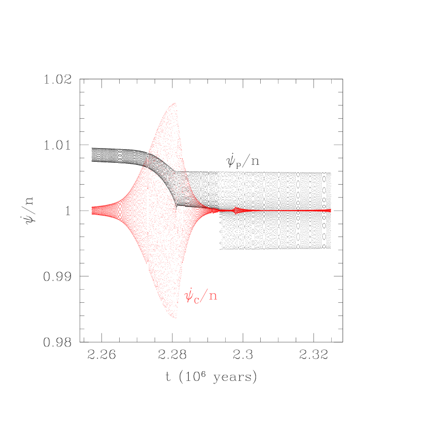
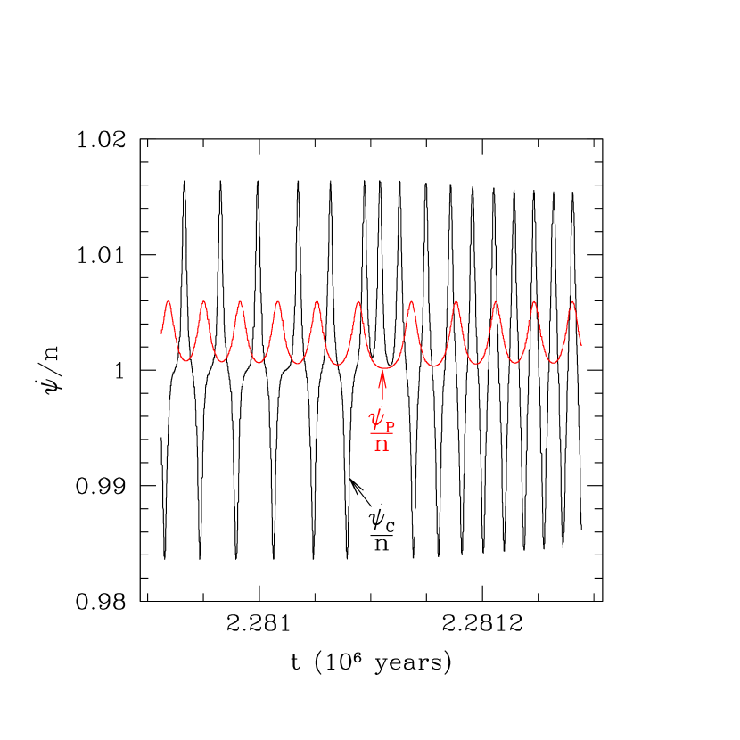
Figure 9: Forced excitation of Charon’s libration about synchronous rotation from an interaction with Pluto’s rotating figure as Pluto approaches synchronous rotation. Initial $e=0.3$, $C_{22i}=10^{-5}$, and $A_{\Delta t}=9$. The left panel shows the growth in amplitude of Charon’s longitude libration as Pluto approaches synchronous rotation, and the right panel shows the transition of the variations in the spin rates as they go out of resonance.

For the cases with non-zero $C_{22i}$ shown in Fig. 8, Charon reaches libration about synchronous rotation before Pluto, and the librations rapidly damp to very small amplitude. However, when Pluto approaches synchronous rotation, the librations of Charon about the synchronous state are forced to significant amplitude. A blowup of these librations are shown in Fig. 9 for the case with $A_{\Delta t}=9$, where the left panel shows $\dot{\psi}_{\scriptscriptstyle C}/n$ and $\dot{\psi}_{\scriptscriptstyle P}/n$ as the latter transitions into synchronous rotation. The graphs are sparsely sampled to see both trends where they are superposed. The variations in the two spins are anti-correlated during the rise in the amplitude of $\dot{\psi}_{\scriptscriptstyle C}$, but that correlation is lost after passage over the peak as shown in the right panel of Fig. 9. The periods of the variation are no longer the same after the peak, and the tides rapidly damp the amplitude of the libration of Charon. It is not until the amplitude is nearly zero that Pluto starts its libration about synchronous rotation, which is damped to zero on a longer time scale. The period of free libration of Charon is approximately 345 days, and that of the variation in $\dot{\psi}_{\scriptscriptstyle C}$ is a little over 400 days. We infer that it is the proximity of the forcing period from the interaction with Pluto’s axial asymmetry with the free period that accounts for the large growth in amplitude. After the peak in the amplitude, the period of Pluto’s rotational variation changes and the two variations are no longer near resonance.

Figure 10: Effects of $C_{22}$ on orbital evolution in the constant $Q$ model. Dotted lines for $C_{22i}=0$ and solid lines for $C_{22i}=10^{-5}$. Initial $e=0.2$, $A_{Q}=0.55$, 0.65, and 0.75 from top to bottom in the eccentricity plot.

Fig. 10 shows the comparison between zero and non-zero $C_{22i}$ in the constant $Q$ model. Initial $e=0.2$ and $A_{Q}=0.55$, $0.65$, and $0.75$ from top to bottom in the eccentricity plot. With non-zero $C_{22i}$, Charon is caught in the 3:2 spin-orbit resonance in all three cases shown here. The eccentricity drops quickly while Charon remains in the resonance, which differs from the zero $C_{22i}$ cases where the eccentricity is roughly constant up to $10^{4}\,$yr. Charon’s spin escapes from the resonance and reaches synchronous rotation when $e$ becomes nearly zero. The nearly zero $e$ also means that Pluto is not captured into any spin-orbit resonance before synchronous rotation is reached (see Section 6.2).

Figure 11: Effects of $C_{22}$ on orbital evolution in the constant $Q$ model with initial $e=0.3$. $C_{22i}=0$ for dotted lines and $10^{-5}$ for solid lines. $A_{Q}=1.13$, 1.14, and 1.15 (lines from top to bottom). The spin of Charon is almost the same in all cases.

As the asymptotic spin rate in the constant $Q$ model is $3n/2$ for $e>0.235$, the spin of Charon can stay at $3n/2$ independent of the value of $C_{22i}$ if the initial $e$ is larger. However, there are differences in the evolution if $C_{22i}$ is non-zero and Charon is actually in the spin-orbit resonance. Fig. 11 compares evolution with zero and non-zero $C_{22i}$ in the constant $Q$ model for initial $e=0.3$ and $A_{Q}=1.13$, 1.14, and 1.15 (lines from top to bottom). The evolution of Charon’s spin is almost the same in all cases, but non-zero $C_{22i}$ causes $e$ to increase quickly here, compared to the cases shown in Fig. 10, where $e$ decreases. (We stopped the calculations with non-zero $C_{22i}$ in Fig. 11 at $t\approx 10^{5}\,$yr, because the evolution equations for constant $Q$ are qualitatively inaccurate for $e\gtrsim 0.36$.) The value of $A_{Q}$ that keeps $e$ roughly constant would change when $C_{22i}$ is non-zero. We find that it is still possible to get a roughly constant $e$ by using a smaller $A_{Q}$ for initial $e=0.2$, and larger $A_{Q}$ for initial $e=0.3$.

6 DISCUSSION

6.1 Tidal Evolution of Pluto-Charon

We discuss in this subsection a number of issues concerning the tidal evolution of Pluto-Charon, including the change of parameters, the use of expanded equations for the constant $Q$ model, and the values of $A$ in the two tidal models.

In Section 5, all results are generated using $\bar{\mathcal{C}}_{\scriptscriptstyle P}=0.328$ and initial $a=4R_{\scriptscriptstyle P}$. We have also performed calculations with other values of $\bar{\mathcal{C}}_{\scriptscriptstyle P}$ and initial $a$, and find that they do not affect our results qualitatively. In particular, it is always possible to find $A$ that keeps $e$ roughly constant throughout most of the evolution.

Figure 12: Evolution using constant $\Delta t$ expanded equations with initial $e=0.2$, $C_{22i}=0$, and $A_{\Delta t}=13$–$18$.

Evolution equations are available in both closed form (Eqs. [3]–[5]) and lowest order expansion in $e$ (Eqs. [20]–[22]) in the constant $\Delta t$ model, while only expanded equations can be obtained for constant $Q$. We compare the results from the two constant $\Delta t$ models to give us an idea how good the results from the $O\left(e^{2}\right)$ equations of the constant $Q$ model are. Fig. 12 shows the evolution using the constant $\Delta t$ expanded equations, with the same initial conditions as in Fig. 4. We find that similar eccentricity evolution can be recovered with the expanded equations by increasing $A_{\Delta t}$. For example, $e$ can be kept more or less constant with $A_{\Delta t}=14$ in Fig. 12, compared to $A_{\Delta t}=10$ in Fig. 4. Larger $A_{Q}$ is also required to keep $e$ more or less constant for larger $e$ in the constant $Q$ model (see, e.g., Fig. 3), which may be a result of truncating the higher order terms in $e$ in the evolution equations. Note, however, that the expanded equations for constant $Q$ are qualitatively inaccurate for $e\gtrsim 0.36$, because they do not give the next discontinuous jump in the asymptotic spin from $3n/2$ to $2n$ (see Section 2.2).

The hypothesis that the small satellites, Nix, Hydra, Keberos, and Styx, were brought to their current orbits by mean-motion resonances with Charon is motivated by finding them currently near the 4:1, 6:1, 5:1, and 3:1 mean-motion commensurabilities with Charon, respectively. As we show in Section 5, $a$ would overshoot the current value if $e$ is large when $a$ reaches this value, and decays back to the current value when $e$ decays. The overshoot poses a problem for the resonant migration hypothesis, as mean-motion resonances may not be sustained with decreasing $a$ of Charon.

Our results show that both tidal models can keep the eccentricity of Charon’s orbit more or less constant during most of the evolution, but that the values of $A$ needed differ by an order of magnitude: $A_{Q}\approx 0.65$–$1.15$ and $A_{\Delta t}\approx 10$. We also show in Fig. 6 that $A_{\Delta t}\approx 3$ would result in unacceptably large eccentricity and growth in $a$ well beyond the current value (especially if $C_{22i}=0$). For both tidal models, we expect $A\approx 0.5$–$3$ if Pluto and Charon have similar tidal response and dissipation. While the values of $A_{Q}$ needed for keeping $e$ roughly constant are reasonable, it is unclear that $A_{\Delta t}\approx 10$ can be achieved with different assumptions about Pluto and Charon. Generally we expect the dissipation in Pluto would be larger than that in Charon (and hence smaller $A$), if Charon comes off more or less intact after the impact. On the other hand, if the differentiated Pluto has fluid Love number $k_{f{\scriptscriptstyle P}}\approx 1$ by analogy with the Earth, while Charon is homogeneous with $k_{f{\scriptscriptstyle C}}=3/2$, the resulting $A$ would be increased by the same factor. Note that $\dot{\psi}_{\scriptscriptstyle P}/n$ is large compared with $\dot{\psi}_{\scriptscriptstyle C}/n$ until close to the end of tidal evolution and the tidal frequencies on Pluto and Charon are different. Unless $A\approx 10$ is plausible, our results suggest that the frequency dependence of the dissipation function $Q$ of real solid materials may be closer to $Q=$ constant than $Q\propto 1/f$ (or constant $\Delta t$).

6.2 Spin-orbit Resonance of Charon

Figure 13: Spin-orbit coupling in the constant $\Delta t$ model. Initial $\dot{\psi}_{\scriptscriptstyle C}=1.9n$ and $A_{\Delta t}=7$, 8.5, 10, and 11.5 (lines from top to bottom).

Figure 14: Spin-orbit coupling in the constant $\Delta t$ model. $A_{\Delta t}=10$ and initial $\dot{\psi}_{\scriptscriptstyle C}/n=3.9$, 2.9, 1.9, and 0.9 (lines from top to bottom).

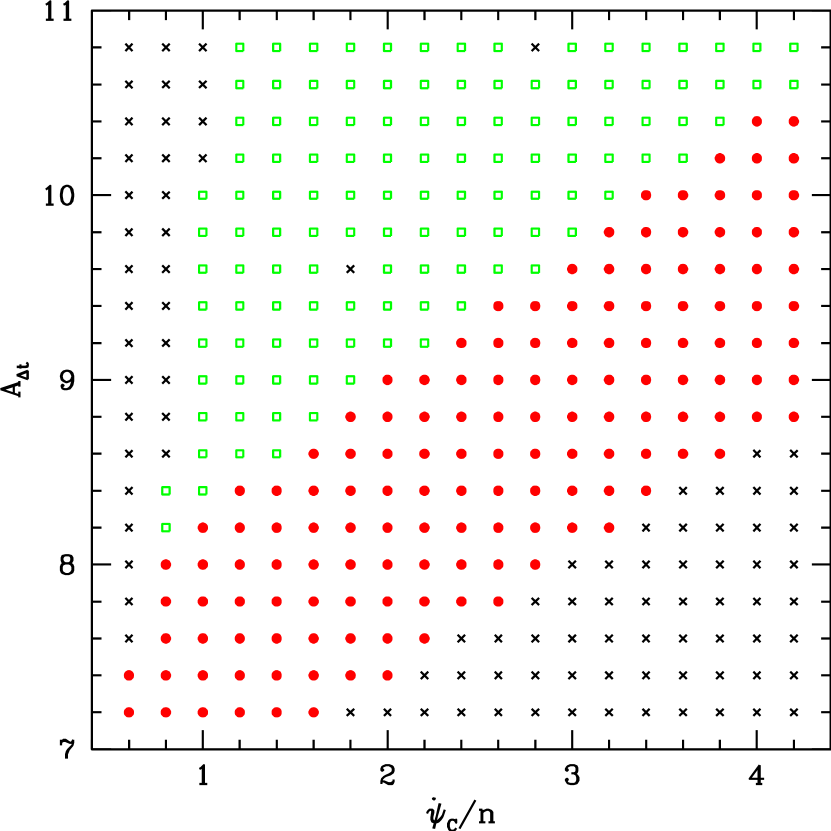
Figure 15: Grid search of 3:2 spin-orbit resonance of Charon in the constant $\Delta t$ model. Initial $e=0.3$, and $A_{\Delta t}$ and initial $\dot{\psi}_{\scriptscriptstyle C}/n$ are varied. Different symbols stand for different results after $t\approx 30$ years: The crosses corresponds to conditions where Charon is not caught in the 3:2 resonance; the open squares where Charon is caught in the 3:2 resonance but escapes before $t\approx 30$ years; and the filled circles where Charon remains in resonance up to $t\approx 30$ years.

In this subsection we discuss in more detail the capture into and escape from spin-orbit resonance for Charon when $C_{22i}$ are non-zero. We focus on the 3:2 spin-orbit resonance, because we are primarily interested in evolution where $e$ does not become too large, and we find only long-term capture into the 3:2 resonance if $e\lesssim 0.36$.

We first consider the constant $\Delta t$ model, where pseudo-synchronous spin of $3n/2$ corresponds to $e\approx 0.285$. Since Charon’s spin quickly reaches the pseudo-synchronous state, $e$ is usually close to the above value when it reaches $3n/2$. Our $C_{22}=10^{-5}$ converts to $(\mathcal{B}-\mathcal{A})/\mathcal{C}=10^{-4}$ for homogeneous body. According to Fig. 6 of Goldreich and Peale (1966) for $(\mathcal{B}-\mathcal{A})/\mathcal{C}=10^{-4}$, the probability for Charon being captured into the 3:2 resonance is close to unity at $e\approx 0.285$. The range of $e$ for certain capture becomes narrower for smaller $C_{22}$ (see their Fig. 7).

Fig. 13 shows the early evolution up to about $30$ years in the constant $\Delta t$ model with initial $e=0.3$, $\dot{\psi}_{\scriptscriptstyle C}=1.9n$, and a range of $A_{\Delta t}$. We see that Charon does not reach the $3n/2$ spin if $A_{\Delta t}$ is small ($\lesssim 7$), and does not stay within the 3:2 resonance for long if $e$ is damped for large $A_{\Delta t}$ ($\gtrsim 10$). Similarly, Fig. 14 shows the early evolution with initial $e=0.3$, $A_{\Delta t}=10$ and a range of initial $\dot{\psi}_{\scriptscriptstyle C}$. Charon does not reach the $3n/2$ spin if the initial $\dot{\psi}_{\scriptscriptstyle C}$ is too small ($\lesssim 1$), and the stability of the resonance is maintained if the initial $\dot{\psi}_{\scriptscriptstyle C}$ is large ($\gtrsim 3.9$) and $e$ remains large. The escape from 3:2 resonance at this stage does not preclude a subsequent capture if $e$ rises above $0.285$ again (see, e.g., Fig. 8).

Fig. 15 shows a grid search for conditions under which Charon stays within the 3:2 spin-orbit resonance in the constant $\Delta t$ model. In these runs, initial $e=0.3$ while $A_{\Delta t}$ and initial $\dot{\psi}_{\scriptscriptstyle C}$ are varied. The initial pointing directions of Pluto and Charon are randomly chosen, and all runs end at $10^{9}$ seconds ($\approx 30$ years). The crosses correspond to those conditions where Charon is not caught in the 3:2 resonance. Charon’s spin never reaches $3n/2$ for the crosses in the upper left and lower right corners, with initial $\dot{\psi}_{\scriptscriptstyle C}$ too low and $e$ too large, respectively. The open squares are those conditions where Charon is caught in the 3:2 resonance but escapes before $t\approx 30$ years, while the filled circles remain in resonance up to that time. For the two crosses surrounded by open squares, it is possible to get them caught in the 3:2 resonance by merely changing the initial pointing directions of Pluto and Charon.

Figure 16: Spin-orbit coupling in the constant $\Delta t$ model. $A_{\Delta t}=10$ and $\Delta t_{\scriptscriptstyle P}=600$, 300, 150, 80, 40, and 20 seconds (lines from top to bottom in the eccentricity plot and from left to right in the other panels).

Figure 17: $\Delta t_{\scriptscriptstyle P}(R_{\scriptscriptstyle P}/a)^{4.5}$ versus the eccentricity at which Charon escapes from the 3:2 spin-orbit resonance for the runs shown in Fig. 16. The straight line is the stability limit Eq. (33) at the lowest order in $e$.

Charon escapes from the spin-orbit resonance if the tidal torque exceeds the maximum possible restoring torque provided by $C_{22}$ on the body. By comparing the torques, the condition for the stability of the 3:2 spin-orbit resonance is (Eq. [6] of Goldreich and Peale 1966):

$$\frac{k_{2C}}{C_{22C}}\frac{M_{\scriptscriptstyle P}^{2}}{M_{\scriptscriptstyle C}(M_{\scriptscriptstyle P}+M_{\scriptscriptstyle C})}\left(\frac{R_{\scriptscriptstyle C}}{a}\right)^{3} < \>\frac{14e}{n\Delta t_{\scriptscriptstyle C}}+O\left(e^{3}\right),$$ (33)

or $$\>14e\ Q_{\scriptscriptstyle C}+O\left(e^{3}\right).$$ (34)

Eq. (33) can be rewritten in terms of $A_{\Delta t}$ and Pluto’s parameters. Fig. 16 shows the evolution for a range of $\Delta t_{\scriptscriptstyle P}$ and $A_{\Delta t}=10$. Charon stays in the 3:2 resonance longer for smaller $\Delta t_{\scriptscriptstyle P}$. To compare with the analytic stability condition, we plot $\Delta t_{\scriptscriptstyle P}(R_{\scriptscriptstyle P}/a)^{4.5}$ against the eccentricity at which Charon leaves the resonance in Fig. 17, so that the $a$ dependence in Eq. (33) is removed. The straight line shows Eq. (33) at the lowest order in $e$. The numerical results agree with the lowest-order analytic theory at small $e$ but show departures at $e\gtrsim 0.2$.

Figure 18: Spin-orbit coupling in the constant $Q$ model. $A_{Q}=0.65$ and initial $e=0.2$, 0.18, 0.16, 0.14, 0.12, and 0.1 (lines from top to bottom).

In the constant $Q$ model, the capture into 3:2 spin-orbit resonance from faster spin is certain if $e>0.235$ and probabilistic if $e<0.235$ (see Fig. 14 of Goldreich and Peale 1966). Fig. 18 illustrates the probabilistic capture using evolution for a range of initial $e$ (0.1–0.2) and $A_{Q}=0.65$. Although all three cases shown in Fig.10 with non-zero $C_{22i}$, initial $e=0.2$, and $A_{Q}=0.55$–$0.75$ show capture into the 3:2 resonance, we do find probabilistic capture when we try other values of $A_{Q}$.

Capture of Charon into spin-orbit resonances other than 3:2 is possible. Fig. 6 shows an example of capture into 2:1 in the constant $\Delta t$ model, but it requires $e$ to exceed $\approx 0.39$. We have also seen temporary captures into 5:4 spin-orbit resonance in more than one case in the constant $\Delta t$ model. We note that Celletti and MacKay (2007) have also seen the 5:4 spin-orbit resonance, and Rodríguez et al. (2012) have seen the 4:3 resonance. The occurrence of these resonances is unexpected from first-order perturbation theory which gives resonances only at spin rates that are half-integer multiples of the mean motion (e.g., Goldreich and Peale 1966). The 5:4 is a second-order resonance that appears in second-order perturbation theory (Flynn and Saha, 2005).

Unlike Charon, Pluto is not captured into any spin-orbit resonance before reaching synchronous rotation in nearly all of our calculations with non-zero $C_{22i}$. Since ${\dot{\psi}}_{P}/n$ is typically $\sim 5$–$6$ initially and rises to $>10$ before falling, by the time ${\dot{\psi}}_{P}/n$ reaches values like $3/2$, the eccentricity is usually below the value where the asymptotic spin rate is $3n/2$, and the probability of capturing Pluto into spin-orbit resonance is small.

In our analysis, we have neglected several effects that could change the probabiliy of capture into various spin-orbit resonances for both Charon and Pluto. These include an alternative tidal dissipation model that combines the Andrade and Maxwell rheological models (e.g., Makarov et al. 2012), core-mantle interactions if the core is liquid (e.g., Peale and Boss 1977; Correia and Laskar 2009), and collisions (e.g., Correia and Laskar 2012). However, even without these additional effects, we already observe the occurrence of such captures for Charon and their effects on the evolutionary track of Pluto-Charon.

7 CONCLUSIONS

We have investigated the tidal evolution of Pluto-Charon on an eccentric orbit under two different tidal models: constant $\Delta t$ and constant $Q$. Our calculations show the complete tidal evolution of a system of two solid bodies of comparable size, where the spin angular momentum of the two bodies is initially comparable to the orbital angular momentum. The deviation from axial symmetry has been included in tidal evolution, and the back reaction on the orbit must be accounted for to conserve angular momentum. Capture into spin-orbit resonances can profoundly affect the tidal evolution of the system.

Motivated by binary asteroids (including those with comparable masses in dual synchronous state, like (69230) Hermes and (90) Antiope), Taylor and Margot (2010, 2011) have studied the tidal evolution of two bodies. They included higher order terms in the tidal potential, but considered only circular orbit and zero $C_{22}$. Rodríguez et al. (2012) have studied the tidal evolution of super-Earths close to their host stars. They considered non-zero $C_{22}$ and eccentric orbit, and also found that capture into spin-orbit resonances can significantly affect the tidal evolution of eccentricity. However, they included only the tides raised by the star on the planet. Both of these studies used the constant $\Delta t$ model only.

The equations used in our study are derived from a variety of existing sources, and we provide a more comprehensive listing of the coefficients in the evolution equations of the constant $Q$ model, which depend discontinuously on the spin rate. In both models, we find the value and range of relative rates of tidal dissipation in Charon to that in Pluto that would result in roughly constant eccentricity during most of the evolution. In the constant $\Delta t$ model, the results are valid for arbitrary eccentricity, which is not true for constant $Q$ (where the results are qualitatively inaccurate for $e\gtrsim 0.36$ due to the necessary truncations in the evolution equations). However, the constant $Q$ model requires a more reasonable relative rate of dissipation between Pluto and Charon ($A_{Q}\sim 1$).

It was assumed in previous studies (e.g., DPH97) that Charon would achieve synchronous rotation quickly after its formation. We show that this is not the case for Charon on an eccentric orbit. The asymptotic spin depends on both the eccentricity and the assumed tidal model. While the inferred large oblateness of Pluto gives no significant change to the evolution, it is found that the capture into spin-orbit resonance of Charon for non-zero values of $C_{22}$ can change the relative dissipation rate that keeps the eccentricity more or less constant during most of the evolution. In some cases (e.g., if $A_{\Delta t}\sim 1$), spin-orbit resonance can allow smooth evolution to the final state of dual synchronous rotation, whereas very large eccentricity and semimajor axis would otherwise occur (which could lead to instability). The conditions of capture into and escape from the 3:2 spin-orbit resonance as a function of the orbital eccentricity agree with the existing results in the literature.

References

- Alexander (1973) Alexander, M.E., 1973. The weak friction approximation and tidal evolution in close binary systems. Ap&SS 23, 459–510.
- Boss and Peale (1986) Boss, A.P., Peale, S.J., 1986. Dynamical constraints on the origin of the Moon, in: W. K. Hartmann, R. J. Phillips, & G. J. Taylor (Ed.), Origin of the Moon, pp. 59–101.
- Buie et al. (2006) Buie, M.W., Grundy, W.M., Young, E.F., Young, L.A., Stern, S.A., 2006. Orbits and Photometry of Pluto’s Satellites: Charon, S/2005 P1, and S/2005 P2. Astron. J. 132, 290–298.
- Buie et al. (2010) Buie, M.W., Grundy, W.M., Young, E.F., Young, L.A., Stern, S.A., 2010. Pluto and Charon with the Hubble Space Telescope. I. Monitoring Global Change and Improved Surface Properties from Light Curves. Astron. J. 139, 1117–1127.
- Buie et al. (2012) Buie, M.W., Tholen, D.J., Grundy, W.M., 2012. The orbit of Charon is circular. Astron. J. 144, 15.
- Buie et al. (1997) Buie, M.W., Tholen, D.J., Wasserman, L.H., 1997. Separate Lightcurves of Pluto and Charon. Icarus 125, 233–244.
- Cameron and Ward (1976) Cameron, A.G.W., Ward, W.R., 1976. The origin of the Moon. Lunar and Planetary Institute Science Conference Abstracts 7, 120.
- Canup (2004) Canup, R.M., 2004. Dynamics of Lunar Formation. Ann. Rev. Astron. Astrophys. 42, 441–475.
- Canup (2005) Canup, R.M., 2005. A giant impact origin of Pluto-Charon. Science 307, 546–550.
- Castillo-Rogez et al. (2011) Castillo-Rogez, J.C., Efroimsky, M., Lainey, V., 2011. The tidal history of Iapetus: Spin dynamics in the light of a refined dissipation model. J. Geophys. Res. (Planets) 116, 9008.
- Celletti and MacKay (2007) Celletti, A., MacKay, R., 2007. Regions of nonexistence of invariant tori for spin-orbit models. Chaos 17, 043119.
- Correia and Laskar (2009) Correia, A.C.M., Laskar, J., 2009. Mercury’s capture into the 3/2 spin-orbit resonance including the effect of core-mantle friction. Icarus 201, 1–11.
- Correia and Laskar (2012) Correia, A.C.M., Laskar, J., 2012. Impact Cratering on Mercury: Consequences for the Spin Evolution. Astrophys. J. 751, L43.
- Dobrovolskis et al. (1997) Dobrovolskis, A.R., Peale, S.J., Harris, A.W., 1997. Dynamics of the Pluto-Charon binary, in: S. A. Stern, & D. J. Tholen (Ed.), Pluto and Charon. Univ. Arizona Press, Tucson, AZ, p. 159.
- Efroimsky and Williams (2009) Efroimsky, M., Williams, J.G., 2009. Tidal torques: a critical review of some techniques. Celest. Mech. Dyn. Astron. 104, 257–289.
- Farinella et al. (1979) Farinella, P., Milani, A., Nobili, A.M., Valsecchi, G.B., 1979. Tidal evolution and the Pluto-Charon system. Moon Planets 20, 415–421.
- Ferraz-Mello et al. (2008) Ferraz-Mello, S., Rodríguez, A., Hussmann, H., 2008. Tidal friction in close-in satellites and exoplanets: The Darwin theory re-visited. Celest. Mech. Dyn. Astron. 101, 171–201.
- Flynn and Saha (2005) Flynn, A.E., Saha, P., 2005. Second-Order Perturbation Theory for Spin-Orbit Resonances. Astron. J. 130, 295–307.
- Gerstenkorn (1955) Gerstenkorn, H., 1955. Über Gezeitenreibung beim Zweikörperproblem. Mit 4 Textabbildungen. Zeitschrift für Astrophysik 36, 245.
- Goldreich (1966) Goldreich, P., 1966. Final spin states of planets and satellites. Astron. J. 71, 1–7.
- Goldreich and Peale (1966) Goldreich, P., Peale, S.J., 1966. Spin-orbit coupling in the solar system. Astron. J. 71, 425–438.
- Greenberg and Weidenschilling (1984) Greenberg, R., Weidenschilling, S.J., 1984. How fast do Galilean satellites spin? Icarus 58, 186–196.
- Hut (1981) Hut, P., 1981. Tidal evolution in close binary systems. Astron. Astrophys. 99, 126–140.
- Kaula (1964) Kaula, W.M., 1964. Tidal dissipation by solid friction and the resulting orbital evolution. Rev. Geophys. Space Phys. 2, 661–685.
- Lee and Peale (2002) Lee, M.H., Peale, S.J., 2002. Dynamics and origin of the 2:1 orbital resonances of the GJ 876 planets. Astrophys. J. 567, 596–609.
- Levison and Duncan (1994) Levison, H.F., Duncan, M.J., 1994. The long-term dynamical behavior of short-period comets. Icarus 108, 18–36.
- Lin (1981) Lin, D.N.C., 1981. On the origin of the Pluto-Charon system. Mon. Not. R. Astron. Soc. 197, 1081–1085.
- Lithwick and Wu (2008) Lithwick, Y., Wu, Y., 2008. On the Origin of Pluto’s Minor Moons, Nix and Hydra. preprint (arXiv:0802.2951) .
- Makarov et al. (2012) Makarov, V.V., Berghea, C., Efroimsky, M., 2012. Dynamical Evolution and Spin-Orbit Resonances of Potentially Habitable Exoplanets: The Case of GJ 581d. Astrophys. J. 761, 83.
- McKinnon (1984) McKinnon, W.B., 1984. On the origin of Triton and Pluto. Nature 311, 355–358.
- McKinnon (1989) McKinnon, W.B., 1989. On the origin of the Pluto-Charon binary. Astrophys. J. 344, L41–L44.
- McKinnon et al. (2008) McKinnon, W.B., Prialnik, D., Stern, S.A., Coradini, A., 2008. Structure and evolution of Kuiper belt objects and dwarf planets, in: Barucci, M. A., Boehnhardt, H., Cruikshank, D. P., & Morbidelli, A. (Ed.), The Solar System Beyond Neptune. Univ. Arizona Press, Tucson, AZ, p. 213.
- Mignard (1979) Mignard, F., 1979. The evolution of the lunar orbit revisited. I. Moon Planets 20, 301–315.
- Mignard (1980) Mignard, F., 1980. The evolution of the lunar orbit revisited. II. Moon Planets 23, 185–201.
- Mignard (1981a) Mignard, F., 1981a. On a possible origin of Charon. Astron. Astrophys. 96, L1.
- Mignard (1981b) Mignard, F., 1981b. The lunar orbit revisited. III. Moon Planets 24, 189–207.
- Munk and MacDonald (1960) Munk, W.H., MacDonald, G.J.F., 1960. The Rotation of the Earth: A Geophysical Discussion. Cambridge Univ. Press, London.
- Murray and Dermott (1999) Murray, C.D., Dermott, S.F., 1999. Solar System Dynamics. Cambridge Univ. Press, Cambridge.
- Peale (1973) Peale, S.J., 1973. Rotation of solid bodies in the solar system. Rev. Geophys. Space Phys. 11, 767–793.
- Peale (1999) Peale, S.J., 1999. Origin and evolution of the natural satellites. Ann. Rev. Astron. Astrophys. 37, 533–602.
- Peale (2005) Peale, S.J., 2005. The free precession and libration of Mercury. Icarus 178, 4–18.
- Peale (2007) Peale, S.J., 2007. The origin of the natural satellites, in: Spohn, T., Schubert, G. (Eds.), Treatise on Geophysics, Vol. 10, Planets and Moons. Elsevier B.V., Amsterdam, p. 465.
- Peale and Boss (1977) Peale, S.J., Boss, A.P., 1977. A spin-orbit constraint on the viscosity of a Mercurian liquid core. J. Geophys. Res. 82, 743–749.
- Peale and Cassen (1978) Peale, S.J., Cassen, P., 1978. Contribution of tidal dissipation to lunar thermal history. Icarus 36, 245–269.
- Peale et al. (1980) Peale, S.J., Cassen, P., Reynolds, R.T., 1980. Tidal dissipation, orbital evolution, and the nature of Saturn’s inner satellites. Icarus 43, 65–72.
- Person et al. (2006) Person, M.J., Elliot, J.L., Gulbis, A.A.S., Pasachoff, J.M., Babcock, B.A., Souza, S.P., Gangestad, J., 2006. Charon’s radius and density from the combined data sets of the 2005 July 11 occultation. Astron. J. 132, 1575–1580.
- Press et al. (1992) Press, W.H., Teukolsky, S.A., Vetterling, W.T., Flannery, B.P., 1992. Numerical Recipes in Fortran 77. The Art of Scientific Computing. Cambridge Univ. Press, Cambridge, Ch. 16.
- Rauch and Holman (1999) Rauch, K.P., Holman, M., 1999. Dynamical chaos in the Wisdom-Holman integrator: Origins and solutions. Astron. J. 117, 1087–1102.
- Rodríguez et al. (2012) Rodríguez, A., Callegari, N., Michtchenko, T.A., Hussmann, H., 2012. Spin-orbit coupling for tidally evolving super-Earths. Mon. Not. R. Astron. Soc. 427, 2239–2250.
- Singer (1968) Singer, S.F., 1968. The origin of the Moon and geophysical consequences. GJRAS 15, 205–226.
- Stern (1992) Stern, S.A., 1992. The Pluto-Charon system. Ann. Rev. Astron. Astrophys. 30, 185–233.
- Taylor and Margot (2010) Taylor, P.A., Margot, J.L., 2010. Tidal evolution of close binary asteroid systems. Celest. Mech. Dyn. Astron. 108, 315–338.
- Taylor and Margot (2011) Taylor, P.A., Margot, J.L., 2011. Binary asteroid systems: Tidal end states and estimates of material properties. Icarus 212, 661–676.
- Tholen et al. (2008) Tholen, D.J., Buie, M.W., Grundy, W.M., Elliott, G.T., 2008. Masses of Nix and Hydra. Astron. J. 135, 777–784.
- Touma and Wisdom (1994a) Touma, J., Wisdom, J., 1994a. Evolution of the Earth-Moon system. Astron. J. 108, 1943–1961.
- Touma and Wisdom (1994b) Touma, J., Wisdom, J., 1994b. Lie-Poisson integrators for rigid body dynamics in the solar system. Astron. J. 107, 1189–1202.
- Touma and Wisdom (1998) Touma, J., Wisdom, J., 1998. Resonances in the early evolution of the Earth-Moon system. Astron. J. 115, 1653–1663.
- Ward and Canup (2006) Ward, W.R., Canup, R.M., 2006. Forced resonant migration of Pluto’s outer satellites by Charon. Science 313, 1107.
- Wisdom and Holman (1991) Wisdom, J., Holman, M., 1991. Symplectic maps for the n-body problem. Astron. J. 102, 1528–1538.
- Yoder and Peale (1981) Yoder, C.F., Peale, S.J., 1981. The tides of Io. Icarus 47, 1–35.
- Zahn (1977) Zahn, J.P., 1977. Tidal friction in close binary stars. Astron. Astrophys. 57, 383–394.