Divide-And-Conquer Computation of Cylindrical Algebraic Decomposition

Abstract.

We present a divide-and-conquer version of the Cylindrical Algebraic Decomposition (CAD) algorithm. The algorithm represents the input as a Boolean combination of subformulas, computes cylindrical algebraic decompositions of solution sets of the subformulas, and combines the results using the algorithm first introduced in [34]. We propose a graph-based heuristic to find a suitable partitioning of the input and present empirical comparison with direct CAD computation.

1. Introduction

A real polynomial system in variables $x_{1},\ldots,x_{n}$ is a formula

$$S(x_{1},\ldots,x_{n})=\bigvee_{1\leq i\leq l}\bigwedge_{1\leq j\leq m}f_{i,j}(x_{1},\ldots,x_{n})\rho_{i,j}0$$

where $f_{i,j}\in\mathbb{R}[x_{1},\ldots,x_{n}]$, and each $\rho_{i,j}$ is one of $<,\leq,\geq,>,=,$ or $\neq$.

A subset of $\mathbb{R}^{n}$ is semialgebraic if it is a solution set of a real polynomial system.

Every semialgebraic set can be represented as a finite union of disjoint cells (see [21]), defined recursively as follows.

• A cell in $\mathbb{R}$ is a point or an open interval.

• A cell in $\mathbb{R}^{k+1}$ has one of the two forms

  $$\{(a_{1},\ldots,a_{k},a_{k+1}):(a_{1},\ldots,a_{k})\in C_{k}\wedge a_{k+1}=r(a_{1},\ldots,a_{k})\}$$

  $$\{(a_{1},\ldots,a_{k},a_{k+1}):(a_{1},\ldots,a_{k})\in C_{k}\wedge r_{1}(a_{1},\ldots,a_{k})<a_{k+1}<r_{2}(a_{1},\ldots,a_{k})\}$$

  where $C_{k}$ is a cell in $\mathbb{R}^{k}$, $r$ is a continuous algebraic function, and $r_{1}$ and $r_{2}$ are continuous algebraic functions, $-\infty$, or $\infty$, and $r_{1}<r_{2}$ on $C_{k}$.

The Cylindrical Algebraic Decomposition (CAD) algorithm [7, 6, 33] can be used to compute a cell decomposition of any semialgebraic set presented by a real polynomial system. An alternative method of computing cell decompositions is given in [12]. Cell decompositions computed by the CAD algorithm can be represented directly [4, 33] as cylindrical algebraic formulas (CAF; a precise definition is given in Section 2).

Example 1.

The following formula $F(x,y,z)$ is a CAF representation of a cell decomposition of the closed unit ball.

$$F(x,y,z) :=( x=-1\wedge y=0\wedge z=0)\vee(-1<x<1\wedge b_{2}(x,y,z))\vee$$

$$(x=1\wedge y=0\wedge z=0)$$

$$b_{2}(x,y,z) := (y=R_{1}(x)\wedge z=0)\vee(R_{1}(x)<y<R_{2}(x)\wedge b_{2,2}(x,y,z))\vee$$

$$(y=R_{2}(x)\wedge z=0)$$

$$b_{2,2}(x,y,z) := z=R_{3}(x,y)\vee R_{3}(x,y)<z<R_{4}(x,y)\vee z=R_{4}(x,y)$$

where

$$R_{1}(x) = Root_{y,1}(x^{2}+y^{2})=-\sqrt{1-x^{2}}$$

$$R_{2}(x) = Root_{y,2}(x^{2}+y^{2})=\sqrt{1-x^{2}}$$

$$R_{3}(x,y) = Root_{z,1}(x^{2}+y^{2}+z^{2})=-\sqrt{1-x^{2}-y^{2}}$$

$$R_{4}(x,y) = Root_{z,2}(x^{2}+y^{2}+z^{2})=\sqrt{1-x^{2}-y^{2}}$$

The CAF representation of a semialgebraic set $A$ can be used to decide whether $A$ is nonempty, to find the minimal and maximal values of the first coordinate of elements of $A$, to generate an arbitrary element of $A$, to find a graphical representation of $A$, to compute the volume of $A$ or to compute multidimensional integrals over $A$ (see [31]).

In our ISSAC conference paper [34] we presented an algorithm, CAFCombine, computing Boolean operations on cylindrical algebraic formulas. In this extended version of the paper we investigate how CAFCombine can be used to construct a divide-and-conquer algorithm for computing a cylindrical algebraic decomposition. The divide-and-conquer algorithm depends on the algorithm Subdivide. Given a real polynomial system $S(x_{1},\ldots,x_{n})$, Subdivide finds a Boolean formula $\Phi$ and real polynomial systems $P_{1},\ldots,P_{m}$ such that

$$S(x_{1},\ldots,x_{n})\Leftrightarrow\Phi(P_{1}(x_{1},\ldots,x_{n}),\ldots,P_{m}(x_{1},\ldots,x_{n}))$$

Algorithm 2.

(DivideAndConquerCAD)
Input: A real polynomial system $S(x_{1},\ldots,x_{n})$.
Output: A cylindrical algebraic formula $F(x_{1},\ldots,x_{n})$ equivalent to $S(x_{1},\ldots,x_{n})$.

1. Use Subdivide to find $\Phi$ and $P_{1},\ldots,P_{m}$ such that

   $$S\Leftrightarrow\Phi(P_{1},\ldots,P_{m})$$

2. If $m=1$ and $P_{1}=S$ then return $CAD(S)$.

3. For $1\leq i\leq m$, compute

   $$F_{i}:=CAD(P_{i})$$

4. Use CAFCombine to compute a CAF $F$ equivalent to

   $$\Phi(F_{1},\ldots,F_{m})$$

5. Return $F$.

The practical usefulness of DivideAndConquerCAD depends on the choice of the algorithm Subdivide. Our experiments suggest that DivideAndConquerCAD is likely to be faster than a direct CAD computation if $\Phi$ is a disjunction and, for any for $i\neq j$, $P_{i}$ and $P_{j}$ contain few polynomials in common. We propose an algorithm Subdivide for polynomial systems $S$ given in disjunctive normal form. The algorithm is based on the connectivity structure of a graph whose vertices are the disjunction terms of $S$ and whose edges depend on polynomials shared between the disjunction terms of $S$.

Example 3.

Let $S(x,y)$ be the result of eliminating the quantifier from

$$S_{0}(x,y) :=\exists z (z^{2}(-151x-740y-642)+z(-39x+285y-634)-241x-$$

$$57y-985<0\wedge z^{2}(275x-144y+128)+z(94x-658y-267)+$$

$$973x-810y+928=0\wedge z^{2}(-310x-224y+144)+$$

$$z(-256x-143y-77)+945x-260y+825\leq 0)$$

using the virtual term substitution algorithm ([36], Mathematica command $Resolve[S_{0},Reals]$). $S(x,y)$ is a disjunction of $43$ conjunctions of polynomial equations and inequalities.
Problem: Find a cell decomposition for the solution set of $S(x,y)$.
Method 1: A direct application of the CAD algorithm. The computation takes $48$ seconds.
Method 2: DivideAndConquerCAD with Subdivide which represents $S(x,y)$ as a disjunction of $43$ subformulas, each subformula equal to one of the conjunctions in $S(x,y)$. The computation takes $8.5$ seconds.
Method 3: DivideAndConquerCAD with graph-based Subdivide which represents $S(x,y)$ as a disjunction of $5$ subformulas. The subformulas are disjunctions of, respectively, $24$, $11,$ $6$, $1$, and $1$ of the conjunctions in $S(x,y)$. The computation takes $2.4$ seconds.

The paper is organized as follows. Section 2 defines cylindrical algebraic formulas. The algorithms CAFCombine and Subdivide are presented in sections 3 and 4. The last section contains experimental data comparing the performance of DivideAndConquerCAD and of direct CAD computation.

2. Cylindrical Algebraic Formulas

Definition 4.

A real algebraic function given by defining polynomial $f\in\mathbb{\mathbb{Z}}[x_{1},\ldots,x_{n},y]$ and root number $p\in\mathbb{N}_{+}$ is the function

(2.1) $$Root_{y,p}f:\mathbb{R}^{n}\ni(x_{1},\ldots,x_{n})\longrightarrow Root_{y,p}f(x_{1},\ldots,x_{n})\in\mathbb{R}$$

where $Root_{y,p}f(x_{1},\ldots,x_{n})$ is the $p$-th real root of $f$ treated as a univariate polynomial in $y$. The function is defined for those values of $x_{1},\ldots,x_{n}$ for which $f(x_{1},\ldots,x_{n},y)$ has at least $p$ real roots. The real roots are ordered by the increasing value, counting multiplicities. A real algebraic number $Root_{y,p}f\in\mathbb{R}$ given by defining polynomial $f\in\mathbb{Z}[y]$ and root number $p$ is the $p$-th real root of $f$. Let $Alg$ be the set of real algebraic numbers and for $C\subseteq\mathbb{R}^{n}$ let $Alg_{C}$ denote the set of all algebraic functions defined and continuous on $C$. (See [28, 31] for more details on how algebraic numbers and functions can be implemented in a computer algebra system.)

Definition 5.

A set $P\subseteq\mathbb{R}[x_{1},\ldots,x_{n},y]$ is delineable over $C\subseteq\mathbb{R}^{n}$ iff

1. $\forall f\in P\>\exists k_{f}\in\mathbb{N\>}\forall a\in C\;\sharp\{b\in\mathbb{R}:f(a,b)=0\}=k_{f}$.

2. For any $f\in P$ and $1\leq p\leq k_{f}$, $Root_{y,p}f$ is a continuous function on $C$.

3. $$\forall f,g\in P (\exists a\in C\>Root_{y,p}f(a)=Root_{y,q}g(a)\Leftrightarrow$$

   $$\forall a\in C\>Root_{y,p}f(a)=Root_{y,q}g(a))$$

Definition 6.

A cylindrical system of algebraic constraints in variables $x_{1},\ldots,x_{n}$ is a sequence $A=(A_{1},\ldots,A_{n})$ satisfying the following conditions.

1. For $1\leq k\leq n$, $A_{k}$ is a set of formulas

   $$A_{k} = \{a_{i_{1},\ldots,i_{k}}(x_{1},\ldots,x_{k}):1\leq i_{1}\leq m\wedge 1\leq i_{2}\leq m_{i_{1}}\wedge\ldots\wedge 1\leq i_{k}\leq m_{i_{1},\ldots,i_{k-1}}\}$$

2. For each $1\leq i_{1}\leq m$, $a_{i_{1}}(x_{1})$ is $true$ or

   $$x_{1}=r$$

   where $r\in Alg$, or

   $$r_{1}<x_{1}<r_{2}$$

   where $r_{1}\in Alg\cup\{-\infty\}$, $r_{2}\in Alg\cup\{\infty\}$ and $r_{1}<r_{2}$. Moreover, if $s_{1},s_{2}\in Alg\cup\{-\infty,\infty\}$, $s_{1}$ appears in $a_{u}(x_{1})$, $s_{2}$ appears in $a_{v}(x_{1})$ and $u<v$ then $s_{1}\leq s_{2}$.

3. Let $k<n$, $I=(i_{1},\ldots,i_{k})$ and let $C_{I}\subseteq\mathbb{R}^{k}$ be the solution set of

   (2.2) $$a_{i_{1}}(x_{1})\wedge a_{i_{1},i_{2}}(x_{1},x_{2})\wedge\ldots\wedge a_{i_{1},\ldots,i_{k}}(x_{1},\ldots,x_{k})$$

   1. For each $1\leq i_{k+1}\leq m_{I}$,

      $$a_{i_{1},\ldots,i_{k},i_{k+1}}(x_{1},\ldots,x_{k},x_{k+1})$$

      is $true$ or

      (2.3) $$x_{k+1}=r(x_{1},\ldots,x_{k})$$

      and $r\in Alg_{C_{I}}$, or

      (2.4) $$r_{1}(x_{1},\ldots,x_{k})<x_{k+1}<r_{2}(x_{1},\ldots,x_{k})$$

      where $r_{1}\in Alg_{C_{I}}\cup\{-\infty\}$, $r_{2}\in Alg_{C_{I}}\cup\{\infty\}$ and $r_{1}<r_{2}$ on $C_{I}$.

   2. If $s_{1},s_{2}\in Alg_{C_{I}}\cup\{-\infty,\infty\}$, $s_{1}$ appears in

      $$a_{i_{1},\ldots,i_{k},u}(x_{1})$$

      $s_{2}$ appears in

      $$a_{i_{1},\ldots,i_{k},v}(x_{1})$$

      and $u<v$ then $s_{1}\leq s_{2}$ on $C_{I}$.

   3. Let $P_{I}\subseteq\mathbb{Z}[x_{1},\ldots,x_{k},x_{k+1}]$ be the set of defining polynomials of all real algebraic functions that appear in formulas $a_{J}$ for $J=(i_{1},\ldots,i_{k},i_{k+1})$, $1\leq i_{k+1}\leq m_{I}$. Then $P_{I}$ is delineable over $C_{I}$.

Definition 7.

Let $A$ be a cylindrical system of algebraic constraints in variables $x_{1},\ldots,x_{n}$. Define

$$b_{i_{1},\ldots,i_{n}}(x_{1},\ldots,x_{n}) := true$$

For $2\leq k\leq n$, level $k$ cylindrical algebraic subformulas given by $A$ are the formulas

$$b_{i_{1},\ldots,i_{k-1}}(x_{1},\ldots,x_{n}):=\bigvee_{1\leq i_{k}\leq m_{i_{1},\ldots,i_{k-1}}}a_{i_{1},\ldots,i_{k}}(x_{1},\ldots,x_{k})\wedge b_{i_{1},\ldots,i_{k}}(x_{1},\ldots,x_{n})$$

The support cell of $b_{i_{1},\ldots,i_{k-1}}$ is the solution set

$$C_{i_{1},\ldots,i_{k-1}}\subseteq\mathbb{R}^{k}$$

of

$$a_{i_{1}}(x_{1})\wedge a_{i_{1},i_{2}}(x_{1},x_{2})\wedge\ldots\wedge a_{i_{1},\ldots,i_{k-1}}(x_{1},\ldots,x_{k-1})$$

The cylindrical algebraic formula (CAF) given by $A$ is the formula

$$F(x_{1},\ldots,x_{n}):=\bigvee_{1\leq i_{1}\leq m}a_{i_{1}}(x_{1})\wedge b_{i_{1}}(x_{1},\ldots,x_{n})$$

Remark 8.

Let $F(x_{1},\ldots,x_{n})$ be a CAF given by a cylindrical system of algebraic constraints $A$. Then

1. For $1\leq k\leq n$, sets $C_{i_{1},\ldots,i_{k}}$ are cells in $\mathbb{R}^{k}$.

2. Cells

   $$\{C_{i_{1},\ldots,i_{n}}:1\leq i_{1}\leq m\wedge 1\leq i_{2}\leq m_{i_{1}}\wedge\ldots\wedge 1\leq i_{n}\leq m_{i_{1},\ldots,i_{n-1}}\}$$

   form a decomposition of the solution set $S_{F}$ of $F$, i.e. they are disjoint and their union is equal to $S_{F}$.

Proof.

Both parts of the remark follow from the definitions of $A$ and $F$.∎

Remark 9.

Given a real polynomial system $S(x_{1},\ldots,x_{n})$ a version of the CAD algorithm can be used to find a CAF $F(x_{1},\ldots,x_{n})$ equivalent to $S(x_{1},\ldots,x_{n})$.

Proof.

The version of CAD described in [33] returns a CAF equivalent to the input system. ∎

3. Algorithm CAFCombine

In this section we describe the algorithm CAFCombine. The algorithm is a modified version of the CAD algorithm. We describe only the modification. For details of the CAD algorithm see [6, 7]. Our implementation is based on the version of CAD described in [33].

Definition 10.

Let $P\subseteq\mathbb{R}[x_{1},\ldots,x_{n}]$ be a finite set of polynomials and let $\overline{P}$ be the set of irreducible factors of elements of $P$. $W=(W_{1},\ldots,W_{n})$ is a projection sequence for $P$ iff

1. Projection sets $W_{1},\ldots,W_{n}$ are finite sets of irreducible polynomials.

2. For $1\leq k\leq n$, $\overline{P}\cap(\mathbb{R}[x_{1},\ldots,x_{k}]\setminus\mathbb{R}[x_{1},\ldots,x_{k-1}])\subseteq W_{k}\subseteq\mathbb{R}[x_{1},\ldots,x_{k}]\setminus\mathbb{R}[x_{1},\ldots,x_{k-1}]$.

3. If $k<n$ and all polynomials of $W_{k}$ have constant signs on a cell $C\subseteq\mathbb{R}^{k}$, then all polynomials of $W_{k+1}$ that are not identically zero on $C\times\mathbb{R}$ are delineable over $C$.

Remark 11.

For an arbitrary finite set $P\subseteq\mathbb{R}[x_{1},\ldots,x_{n}]$ a projection sequence can be computed using Hong’s projection operator [14]. McCallum’s projection operator [23, 24] gives smaller projection sets for well-oriented sets $P$.

If $P\subseteq Q\subseteq\mathbb{R}[x_{1},\ldots,x_{n}]$ and $W$ is a projection sequence for $Q$ then $W$ is a projection sequence for $P$.

Notation 12.

For a CAF $F$, let $P_{F}$ denote the set of defining polynomials of all algebraic numbers and functions that appear in $F$ .

First let us prove the following rather technical effective lemmas that will be used in the algorithm. We use notation of Definition 7.

Lemma 13.

Let

$$F(x_{1},\ldots,x_{n}):=\bigvee_{1\leq i_{1}\leq m}a_{i_{1}}(x_{1})\wedge b_{i_{1}}(x_{1},\ldots,x_{n})$$

be a CAF and let $-\infty=r_{0}<r_{1}<\ldots<r_{l}<r_{l+1}=\infty$ be such that all real roots of elements of $P_{F}\cap\mathbb{R}[x_{1}]$ are among $r_{1},\ldots,r_{l}$. Let $a(x_{1})$ be either $x_{1}=r_{j}$ for some $1\leq j\leq l$, or $r_{j}<x_{1}<r_{j+1}$ for some $0\leq j\leq l$, and let $C_{a}$ be the solution set of $a$. Then

(3.1) $$\forall x_{1}\in C_{a}\>F(x_{1},\ldots,x_{n})\Leftrightarrow G(x_{1},\ldots,x_{n})$$

and one of the following two statements is true

1. There exist $1\leq i_{1}\leq m$ such that $C_{a}\subseteq C_{i_{1}}$ and $G(x_{1},\ldots,x_{n})=b_{i_{1}}(x_{1},\ldots,x_{n})$.

2. For all $1\leq i_{1}\leq m$, $C_{a}\cap C_{i_{1}}=\emptyset$ and $G(x_{1},\ldots,x_{n})=false$

Moreover, given $F$ and $a$, $G$ can be found algorithmically.

Proof.

Let $r$ be an algebraic number that appears in $a_{i_{1}}$. Then $r=Root_{x_{1},p}f$ for some $f\in P_{F}$. Hence, $r=r_{j_{0}}$ for some $1\leq j_{0}\leq l$ and the value of $j_{0}$ can be determined algorithmically. If $a$ is $x_{1}=r_{j}$, then $C_{a}\cap C_{i_{1}}\neq\emptyset$ iff $a_{i_{1}}$ is either $x_{1}=r_{j}$ or $r_{u}<x_{1}<r_{v}$ with $u<j<v$. In both cases $C_{a}\subseteq C_{i_{1}}$. If $a$ is $r_{j}<x_{k}<r_{j+1}$, then $C_{a}\cap C_{i_{1}}\neq\emptyset$ iff $a_{i_{1}}$ is $r_{u}<x_{1}<r_{v}$ with $u\leq j$ and $v\geq j+1$. In this case also $C_{a}\subseteq C_{i_{1}}$. Equivalence (3.1) follows from the statements (1) and (2).∎

Lemma 14.

Let $2\leq k\leq n$, let

$$b_{i_{1},\ldots,i_{k-1}}(x_{1},\ldots,x_{n}) := \bigvee_{1\leq i_{k}\leq m_{i_{1},\ldots,i_{k-1}}}a_{i_{1},\ldots,i_{k}}(x_{1},\ldots,x_{k})\wedge b_{i_{1},\ldots,i_{k}}(x_{1},\ldots,x_{n})$$

be a level $k$ cylindrical algebraic subformula of a CAF $F$, let $W=(W_{1},\ldots,W_{n})$ be a projection sequence for $P_{F}$. Let $C\subseteq\mathbb{R}^{k-1}$ be a cell such that all polynomials of $W_{k-1}$ have constant signs on $C$ and $C\subseteq C_{i_{1},\ldots,i_{k-1}}$. Let $(c_{1},\ldots,c_{k-1})\in C$ and let $d_{1}<\ldots<d_{l}$ be all real roots of $\{f(c_{1},\ldots,c_{k-1},x_{k}):f\in W_{k}\}$. For $1\leq j\leq l$, let $r_{j}:=Root_{x_{k},p}f$, where $f\in W_{k}$ and $d_{j}$ is the $p$-th root of $f(c_{1},\ldots,c_{k-1},x_{k})$. Let $a(x_{1},\ldots,x_{k})$ be either $x_{k}=r_{j}$ for some $1\leq j\leq l$, or $r_{j}<x_{k}<r_{j+1}$ for some $0\leq j\leq l$, where $r_{0}:=-\infty$ and $r_{l+1}:=\infty$ and let

$$C_{a}:=\{(x_{1},\ldots,x_{k}):(x_{1},\ldots,x_{k-1})\in C\wedge a(x_{1},\ldots,x_{k})\}$$

Then

(3.2) $$\forall(x_{1},\ldots,x_{k})\in C_{a}\>b_{i_{1},\ldots,i_{k-1}}(x_{1},\ldots,x_{n})\Leftrightarrow G(x_{1},\ldots,x_{n})$$

and one of the following two statements is true

1. There exist $1\leq i_{k}\leq m_{i_{1},\ldots,i_{k-1}}$ such that

   $$C_{a}\subseteq C_{i_{1},\ldots,i_{k-1},i_{k}}$$

   and

   $$G(x_{1},\ldots,x_{n})=b_{i_{1},\ldots,i_{k}}(x_{1},\ldots,x_{n})$$

2. For all $1\leq i_{k}\leq m_{i_{1},\ldots,i_{k-1}}$

   $$C_{a}\cap C_{i_{1},\ldots,i_{k-1},i_{k}}=\emptyset$$

   and

   $$G(x_{1},\ldots,x_{n})=false$$

Moreover, given $b_{i_{1},\ldots,i_{k-1}}$, $a$, $(c_{1},\ldots,c_{k-1})$, $d_{1},\ldots,d_{l}$ and the multiplicity of $d_{j}$ as a root of $f$, for all $1\leq j\leq l$ and $f\in W_{k}$, $G$ can be found algorithmically.

Proof.

Let $r$ be an algebraic function that appears in $a_{i_{1},\ldots,i_{k}}$. Then $r=Root_{x_{k},p}f$ for some $f\in P_{F}$. By Definition 6, $r$ is defined and continuous on $C$. Since $W$ is a projection sequence for $P_{F}$, all factors of $f$ that depend on $x_{k}$ are elements of $W_{k}$. Hence, $r(c_{1},\ldots,c_{k-1})=d_{j_{0}}$ for some $1\leq j_{0}\leq l$. Since $d_{j_{0}}$ is the $p$-th of real roots of factors of $f$, multiplicities counted, if the multiplicity of $d_{j}$ as a root of $f$ is known for all $1\leq j\leq l$ and $f\in W_{k}$, the value of $j_{0}$ can be determined algorithmically. Since all polynomials of $W_{k-1}$ have constant signs on $C$, all elements of $W_{k}$ that are not identically zero on $C$ are delineable over $C$. Therefore, $r=r_{j_{0}}$ and $r_{1}<\ldots<r_{l}$ on $C$. If $a$ is $x_{k}=r_{j}$, then $C_{a}\cap C_{i_{1},\ldots,i_{k-1},i_{k}}\neq\emptyset$ iff $a_{i_{1},\ldots,i_{k}}$ is either $x_{k}=r_{j}$ or $r_{u}<x_{k}<r_{v}$ with $u<j<v$. In both cases $C_{a}\subseteq C_{i_{1},\ldots,i_{k-1},i_{k}}$. If $a$ is $r_{j}<x_{k}<r_{j+1}$, then $C_{a}\cap C_{i_{1},\ldots,i_{k-1},i_{k}}\neq\emptyset$ iff $a_{i_{1},\ldots,i_{k}}$ is $r_{u}<x_{k}<r_{v}$ with $u\leq j$ and $v\geq j+1$. In this case also $C_{a}\subseteq C_{i_{1},\ldots,i_{k-1},i_{k}}$. Equivalence (3.2) follows from the statements (1) and (2). ∎

Let us now describe two subalgorithms used in CAFCombine. The first, recursive, subalgorithm requires its input to satisfy the following conditions.

1. $W=(W_{1},\ldots,W_{n})$ is a projection sequence for $P_{F_{1}}\cup\ldots\cup P_{F_{m}}$, where

   $$F_{1}(x_{1},\ldots,x_{n}),\ldots,F_{m}(x_{1},\ldots,x_{n})$$

   are cylindrical algebraic formulas.

2. $(c_{1},\ldots,c_{k-1})\in C$, $2\leq k\leq n$ and $C\subseteq\mathbb{R}^{k-1}$ is a cell such that all polynomials of $W_{k-1}$ have constant signs on $C$.

3. Each $B_{j}$ is a level $k$ cylindrical algebraic formula of $F_{j}$ or $false$.

4. $C$ is contained in the intersection of support cells of all $B_{j}$ that are not $false$.

5. $\Phi(p_{1},\ldots,p_{m})$ is a Boolean formula.

Algorithm 15.

(Lift)
Input: $(c_{1},\ldots,c_{k-1})\in\mathbb{R}^{k-1}$, $W$, $B_{1},\ldots,B_{m}$, $\Phi$.
Output: A level $k$ cylindrical algebraic subformula

$$b(x_{1},\ldots,x_{n})$$

such that

(3.3) $$\forall(x_{1},\ldots,x_{k-1})\in C\>b(x_{1},\ldots,x_{n})\Leftrightarrow\Phi(B_{1}(x_{1},\ldots,x_{n}),\ldots,B_{m}(x_{1},\ldots,x_{n}))$$

1. Let $d_{1}<\ldots<d_{l}$ be all real roots of

   $$\{f(c_{1},\ldots,c_{k-1},x_{k}):f\in W_{k}\}$$

2. For $1\leq i\leq l$, let $r_{i}:=Root_{x_{k},p}f$, where $f\in W_{k}$ and $d_{i}$ is the $p$-th root of $f(c_{1},\ldots,c_{k-1},x_{k})$.

3. For $f\in W_{k}$, if $d_{i}$ is a root of $f(c_{1},\ldots,c_{k-1},x_{k})$, let $M(f,i)$ be its multiplicity, otherwise $M(f,i):=0$.

4. For $1\leq i\leq l$, set $a_{2i}(x_{1},\ldots,x_{k}):=(x_{k}=r_{i})$ and $c_{k,2i}:=d_{i}$.

5. For $0\leq i\leq l,$ set

   $$a_{2i+1}(x_{1},\ldots,x_{k}):=(r_{i}<x_{k}<r_{i+1})$$

   where $r_{0}:=-\infty$ and $r_{l+1}:=\infty$, and pick $c_{k,2i+1}\in(d_{i},d_{i+1})\cap\mathbb{Q}$, where $d_{0}:=-\infty$ and $d_{l+1}:=\infty$.

6. For $1\leq i\leq 2l+1$

   1. For $1\leq j\leq m$, if $B_{j}=false$, set $G_{j}=false$, otherwise let $G_{j}$ be the formula $G$ found using Lemma 14 applied to $B_{j}$, $a_{i}$, $(c_{1},\ldots,c_{k-1})$,
      $d_{1},\ldots,d_{l}$ and $M$.

   2. Let $\Psi:=\Phi(G_{1},\ldots,G_{m})$. If $\Psi$ is $true$ or $false$, set $b_{i}(x_{1},\ldots,x_{n}):=\Psi$.

   3. Otherwise set $b_{i}(x_{1},\ldots,x_{n})$ to

      $$Lift((c_{1},\ldots,c_{k-1},c_{k,i}),W,G_{1},\ldots,G_{m},\Phi)$$

7. Return

   $$b(x_{1},\ldots,x_{n}):=\bigvee_{1\leq i\leq 2l+1}a_{i}(x_{1},\ldots,x_{k})\wedge b_{i}(x_{1},\ldots,x_{n})$$

The second subalgorithm requires its input to satisfy the following conditions.

1. Either $a(x_{1})=(x_{1}=r)$, where $r\in Alg$, or $a(x_{1})=(r<x_{1}<s)$, where $r\in Alg\cup\{-\infty\}$ and $s\in Alg\cup\{\infty\}$.

2. For $1\leq j\leq m$, $B_{j}$ is a level $2$ cylindrical algebraic subformula of a CAF

   $$F_{j}(x_{1},\ldots,x_{n}):=a(x_{1})\wedge B_{j}(x_{1},\ldots,x_{n})$$

3. $\Phi(p_{1},\ldots,p_{m})$ is a Boolean formula.

Algorithm 16.

(CombineStacks)
Input: $a$, $B_{1},\ldots,B_{m}$, $\Phi$.
Output: A CAF $F(x_{1},\ldots,x_{n})$ such that

(3.4) $$F(x_{1},\ldots,x_{n})\Longleftrightarrow\Phi(F_{1}(x_{1},\ldots,x_{n}),\ldots,F_{m}(x_{1},\ldots,x_{n}))$$

1. Let $W:=(W_{1},\ldots,W_{n})$ be a projection sequence for $P_{F_{1}}\cup\ldots\cup P_{F_{m}}$.

2. If $a(x_{1})=(x_{1}=r)$ then set $l:=0$, $a_{1}(x_{1}):=(x_{1}=r)$, and $c_{1,1}:=r$.

3. If $a(x_{1})=(r<x_{1}<s)$ then

   1. Let $r_{1}<\ldots<r_{l}$ be all real roots of elements of $W_{1}$ in $(r,s)$.

   2. For $1\leq i\leq l,$ set $a_{2i}(x_{1}):=(x_{1}=r_{i})$ and $c_{1,2i}:=r_{i}$.

   3. For $0\leq i\leq l,$ set $a_{2i+1}(x_{1}):=(r_{i}<x_{1}<r_{i+1})$ and pick $c_{1,2i+1}\in(r_{i},r_{i+1})\cap\mathbb{Q}$, where $r_{0}:=r$ and $r_{l+1}:=s$.

4. For $1\leq i\leq 2l+1$ set

   $$b_{i}(x_{1},\ldots,x_{n}):=Lift((c_{1,i}),W,B_{1},\ldots,B_{m},\Phi)$$

5. Return

   $$F(x_{1},\ldots,x_{n}):=\bigvee_{1\leq i\leq 2l+1}a_{i}(x_{1})\wedge b_{i}(x_{1},\ldots,x_{n})$$

We can now describe the algorithm CADCombine (cf. [34], Algorithm 17).

Algorithm 17.

(CAFCombine)
Input: Cylindrical algebraic formulas

$$F_{1}(x_{1},\ldots,x_{n}),\ldots,F_{m}(x_{1},\ldots,x_{n})$$

and a Boolean formula $\Phi(p_{1},\ldots,p_{m})$.
Output: A CAF $F(x_{1},\ldots,x_{n})$ such that

(3.5) $$F(x_{1},\ldots,x_{n})\Longleftrightarrow\Phi(F_{1}(x_{1},\ldots,x_{n}),\ldots,F_{m}(x_{1},\ldots,x_{n}))$$

1. Let $r_{1}<\ldots<r_{l}$ be all real roots of $(P_{F_{1}}\cup\ldots\cup P_{F_{m}})\cap\mathbb{R}[x_{1}]$.

2. For $1\leq i\leq l,$ set $a_{2i}(x_{1}):=(x_{1}=r_{i})$ and for $0\leq i\leq l,$ set $a_{2i+1}(x_{1}):=(r_{i}<x_{1}<r_{i+1})$, where $r_{0}:=-\infty$ and $r_{l+1}:=\infty$.

3. For $1\leq i\leq 2l+1$

   1. For $1\leq j\leq m$, let $G_{j}$ be the formula $G$ found using Lemma 13 applied to $F_{j}$ and $a_{i}$.

   2. Let $j_{1},\ldots,j_{s}$ be all $1\leq j\leq m$ for which $G_{j}$ is neither $true$ nor $false$.

   3. Let $\Psi(p_{j_{1}},\ldots p_{j_{s}})$ be the formula obtained from $\Phi$ by replacing $p_{j}$ with $G_{j}$ for all $j$ for which $G_{j}$ is $true$ or $false$.

   4. If $\Psi$ is $true$ or $false$, set $H_{i}(x_{1},\ldots,x_{n}):=a_{i}\wedge\Psi$.

   5. Otherwise set $H_{i}(x_{1},\ldots,x_{n})$ to

      $$CombineStacks(a_{i};G_{j_{1}},\ldots,G_{j_{s}};\Psi)$$

4. Return $F(x_{1},\ldots,x_{n}):=\bigvee_{1\leq i\leq 2l+1}H_{i}(x_{1},\ldots,x_{n})$.

Proof.

(Correctness of the algorithms) To show correctness of CombineStacks, let us first show that inputs to Lift satisfy the required conditions. Condition (1) follows from step 1 of CombineStacks. If $k=2$, the cell $C$ is defined as a root or the open interval between two subsequent roots of polynomials of $W_{1}$. For $k>2$, the cell $C$ is defined as a graph of a root or the set between graphs of two subsequent roots of polynomials of $W_{k-1}$ over a cell on which $W_{k-1}$ is delineable. This proves condition (2). Conditions (3) and (4) are guaranteed by Lemmas 13 and 14. Finally, (5) is satisfied, because $\Phi$ is always the same formula, given as input to CombineStacks.

To complete the proof we need to show the equivalences (3.4) and (3.3). Equivalence (3.3) follows from Lemma 14 and the fact that the sets

$$\{(x_{1},\ldots,x_{k}):(x_{1},\ldots,x_{k-1})\in C\wedge a_{i}(x_{1},\ldots,x_{k})\}$$

are disjoint and their union is equal to $C\times\mathbb{R}$. Equivalence (3.4) follows from Lemma 13 and the fact that the sets $\{x_{1}\in\mathbb{R}:a_{i}(x_{1})\}$ are disjoint and their union is equal to $\mathbb{R}$.

Correctness of CAFCombine follows from Lemma 13, correctness of CombineStacks, and the fact that the sets $\{x_{1}\in\mathbb{R}:a_{i}(x_{1})\}$ are disjoint and their union is equal to $\mathbb{R}$. ∎

Example 18.

Let

$$f_{1} := (x+1)^{4}+y^{4}-4$$

$$g_{1} := (x+2)^{2}+y^{2}-5$$

$$f_{2} := (x-1)^{4}+y^{4}-4$$

$$g_{2} := (x-2)^{2}+y^{2}-5$$

and let

$$A_{1} := \{(x,y)\in\mathbb{R}^{2}\>:\>f_{1}<0\wedge g_{1}<0\}$$

$$A_{2} := \{(x,y)\in\mathbb{R}^{2}\>:\>f_{2}<0\wedge g_{2}<0\}$$

The following CAFs represent cell decompositions of $A_{1}$ and $A_{2}$.

$$F_{1}(x,y) := r_{1}<x<r_{2}\wedge Root_{y,1}f_{1}<y<Root_{y,2}f_{1}\vee$$

$$x=r_{2}\wedge Root_{y,1}f_{1}<y<Root_{y,2}f_{1}\vee$$

$$r_{2}<x<r_{4}\wedge Root_{y,1}g_{1}<y<Root_{y,2}g_{1}$$

$$F_{2}(x,y) := r_{3}<x<r_{5}\wedge Root_{y,1}g_{2}<y<Root_{y,2}g_{2}\vee$$

$$x=r_{5}\wedge Root_{y,1}g_{2}<y<Root_{y,2}g_{2}\vee$$

$$r_{5}<x<r_{6}\wedge Root_{y,1}f_{2}<y<Root_{y,2}f_{2}$$

where

$$r_{1} := -1-\sqrt{2}\approx-2.414$$

$$r_{2} := Root_{x,1}x^{4}+6x^{3}+10x^{2}-2x-1\approx-0.244$$

$$r_{3} := 2-\sqrt{5}\approx-0.236$$

$$r_{4} := -2+\sqrt{5}\approx 0.236$$

$$r_{5} := Root_{x,2}x^{4}-6x^{3}+10x^{2}+2x-1\approx 0.244$$

$$r_{6} := 1+\sqrt{2}\approx 2.414$$

Compute a CAF representation of $A_{1}\cap A_{2}$ (Figure 1) using CAFCombine.

The input consists of $F_{1}$, $F_{2}$ and $\Phi(p_{1},p_{2}):=p_{1}\wedge p_{2}$. The roots computed in step (1) are $r_{1}$, $r_{2}$, $r_{3}$, $r_{4}$, $r_{5}$ and $r_{6}$. In step (3), for all $i\neq 7$, either $G_{1}$ or $G_{2}$ is $false$, and hence $\Psi=false$. For $i=7$ the algorithm computes $CombineStacks(a_{7};G_{1},G_{2};\Phi)$, where

$$a_{7} := r_{3}<x<r_{4}$$

$$G_{1} := Root_{y,1}g_{1}<y<Root_{y,2}g_{1}$$

$$G_{2} := Root_{y,1}g_{2}<y<Root_{y,2}g_{2}$$

The projection sequence computed in step (1) of CombineStacks is

$$W_{2} := \{g_{1},g_{2}\}$$

$$W_{1} := \{x,x^{2}+4x-1,x^{2}-4x-1\}$$

The only root of $W_{1}$ in $(r_{3},r_{4})$ is $0$. The returned cell decomposition of $A_{1}\cap A_{2}$ consists of three cells constructed by Lift over cells $r_{3}<x<0$, $x=0$, and $0<x<r_{4}$.

$$F(x,y) := r_{3}<x<0\wedge Root_{y,1}g_{2}<y<Root_{y,2}g_{2}\vee$$

$$x=0\wedge-1<y<1\vee$$

$$0<x<r_{4}\wedge Root_{y,1}g_{1}<y<Root_{y,2}g_{1}$$

Note that the computation did not require including $f_{1}$ and $f_{2}$ in the projection set.

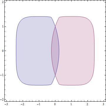
Figure 3.1. Sets $A_{1}$ and $A_{2}$

4. Algorithm Subdivide

In this section we propose an algorithm for subdividing polynomial systems $S(x_{1},\ldots,x_{n})$ given in disjunctive normal form. From experimenting with various subdivision methods we deduced the following rules for designing a subdivision heuristic.

• Do not subdivide conjunctions.

• Group terms of the disjunction so that different groups have as few common polynomials as possible.

• Common polynomials that contain $x_{n}$ matter much more than polynomials that do not contain $x_{n}$.

• Common polynomials with higher degrees in $x_{n}$ matter more than polynomials with lower degrees in $x_{n}$.

This led us to the following subdivision algorithm. The algorithm depends on a parameter $0\leq p\leq 1$ to be determined experimentally.

Notation 19.

Let $S(x_{1},\ldots,x_{n})$ and $T(x_{1},\ldots,x_{n})$ be real polynomial systems. Let $Wt(S)$ denote the sum of degrees in $x_{n}$ of all distinct polynomials that appear in $S$, and let $Wt(S,T)$ denote the sum of degrees in $x_{n}$ of all distinct polynomials that appear both in $S$ and in $T$.

Algorithm 20.

(Subdivide)
Input: A real polynomial system $S(x_{1},\ldots,x_{n})$.
Output: A Boolean formula $\Phi$ and real polynomial systems $P_{1},\ldots,P_{m}$ such that

$$S(x_{1},\ldots,x_{n})\Leftrightarrow\Phi(P_{1}(x_{1},\ldots,x_{n}),\ldots,P_{m}(x_{1},\ldots,x_{n}))$$

1. If $S$ is not a disjunction return $\Phi:=Id$ and $P_{1}:=S$.

2. Let $S=S_{1}\vee\ldots\vee S_{k}$. Construct a graph $G$ as follows.

   1. The vertices of $G$ are $S_{1},\ldots,S_{k}$.

   2. There is an edge connecting $S_{i}$ and $S_{j}$ if $Wt(S_{i},S_{j})>0$ and

      $$Wt(S_{i},S_{j})\geq p\min(Wt(S_{i}),Wt(S_{j}))$$

3. Compute the connected components $\{S_{1,1},\ldots,S_{1,l_{1}}\},\ldots,\{S_{m,1},\ldots,S_{m,l_{m}}\}$ of $G$.

4. For $1\leq j\leq m$ set $P_{j}:=S_{j,1}\vee\ldots\vee S_{j,l_{j}}$.

5. Set $\Phi(p_{1},\ldots,p_{m}):=p_{1}\vee\ldots\vee p_{m}$

6. Return $\Phi$ and $P_{1},\ldots,P_{m}$.

5. Empirical Results

In this section we compare performance of DivideAndConquerCAD and of direct CAD computation. As benchmark problems we chose formulas obtained by application of virtual term substitution methods to quantifier elimination problems, because such formulas are “naturally occurring” CAD inputs that are disjunctions of many terms. We ran four variants of DivideAndConquerCAD, corresponding to different choices of the parameter $p$ in Subdivide. We used $p=0.25$, $p=0.5$, $p=0.75$, and $p=1$. The algorithms have been implemented in C, as a part of the kernel of Mathematica. For direct CAD computation the algorithms use the Mathematica implementation of the version of CAD described in [33]. The experiments have been conducted on a Linux virtual machine with a $3.07$ GHz Intel Core i7 processor and $6$ GB of RAM available. Each computation was given a time limit of $1200$ seconds.

5.1. Examples from [5]

In [5] there are 56 examples obtained by application of virtual term substitution methods to quantifier elimination problems. Here we used 28 of the examples, 7 from applications and 21 randomly generated, for which there were between 2 and 4 free variables. In 22 of the 28 examples at least one method finished within the time limit and the difference between the slowest and the fastest timing was at least $10\%$. In 10 of the 22 examples the input systems were subdivided only for $p=1$, and DivideAndConquerCAD with $p=1$ was slower than direct CAD computation. Timings for the remaining 12 examples are shown in Figure 5.1 (note the logarithmic scale). In 9 of the 12 examples DivideAndConquerCAD with $p=0.75$ is faster than direct CAD computation, in 3 examples it is slower. In the 12 examples DivideAndConquerCAD with $p=0.75$ is the fastest method on average, $2.25$ times faster than direct CAD computation.

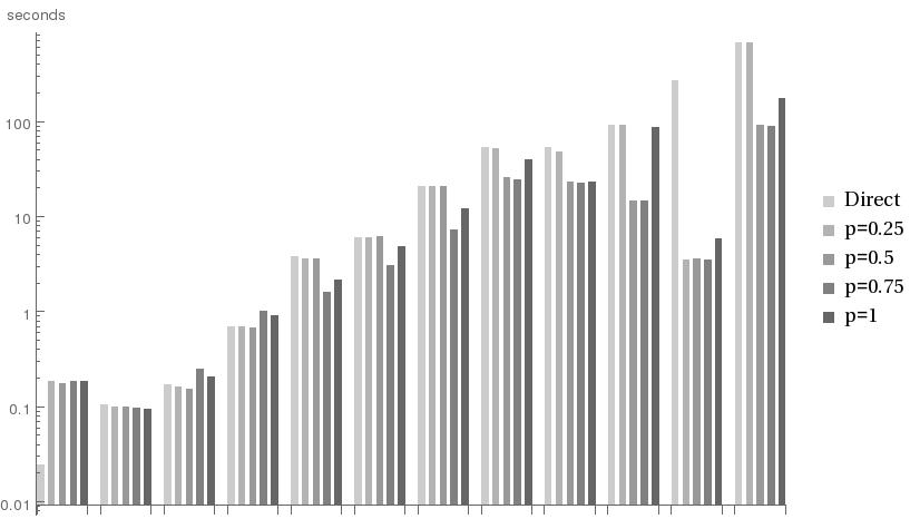
Figure 5.1. Examples from [5]

5.2. Random examples

We generated 16 random examples with 2 or 3 variables. The examples were obtained by elimination of up to three quantifiers using virtual term substitution (with intermediate formula simplification). The initial quantified systems were randomly generated quantified conjunctions of 2-4 polynomial equations or inequalities. The polynomials were linear in all quantified variables except for the first one and quadratic in the remaining variables. The quadratic term in the first quantifier variable did not contain other quantifier variables. The results of quantifier elimination were put in disjunctive normal form and only disjunctions of at least 10 terms were selected. In 2 examples all timings were the same. Timings for the remaining 14 examples are shown in Figure 5.2 (note the logarithmic scale). In 12 of the 14 examples DivideAndConquerCAD with $p=0.75$ is faster than direct CAD computation, in one example it is slower. In the 14 examples DivideAndConquerCAD with $p=0.75$ is the fastest method on average, at least $3.96$ times faster than direct CAD computation (in two examples direct CAD computation did not finish in $1200$ seconds and DivideAndConquerCAD with $p=0.75$ did).

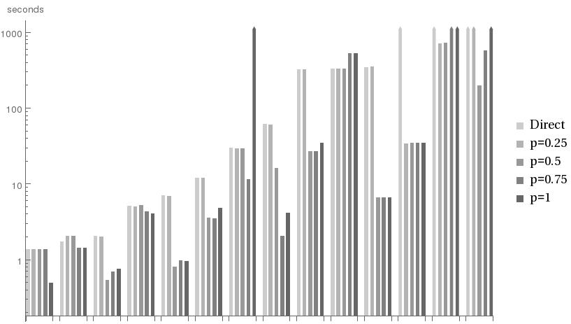
Figure 5.2. Random examples

5.3. Conclusions

The experiments show that DivideAndConquerCAD with graph-based Subdivide is often, but not always, faster than direct CAD computation. On average, the best performance was obtained by choosing the parameter value $p=0.75$ in Subdivide.

References

- [1] H. Anai, K. Yokoyama, “CAD via Numerical Computation with Validated Symbolic Reconstruction, A3L 2005 Proceedings, 2005, 25-30.
- [2] C. W. Brown, “Improved Projection for Cylindrical Algebraic Decomposition”, J. Symbolic Comp., 32 (2001), 447-465.
- [3] C. W. Brown, “An Overview of QEPCAD B: a Tool for Real Quantifier Elimination and Formula Simplification”, J. JSSAC, Vol 10, No. 1 (2003), 13-22.
- [4] C. W. Brown, “QEPCAD B - a program for computing with semi-algebraic sets using CADs”, ACM SIGSAM Bulletin, 37 (4), 2003, 97-108.
- [5] C. W. Brown, A. Strzebonski, Black-Box/White-Box Simplification and Applications to Quantifier Elimination, Proceedings of the International Symposium on Symbolic and Algebraic Computation, ISSAC 2010, 69-76, Munich, Germany, July 25-28, 2010. ACM, Stephen M. Watt, ed.
- [6] B. Caviness, J. Johnson (eds.), “Quantifier Elimination and Cylindrical Algebraic Decomposition”, Springer-Verlag 1998.
- [7] G. E. Collins, “Quantifier Elimination for the Elementary Theory of Real Closed Fields by Cylindrical Algebraic Decomposition”, Lect. Notes Comput. Sci., 33, 1975, 134-183.
- [8] G. E. Collins, “Quantifier Elimination by Cylindrical Algebraic Decomposition - Twenty Years of Progress”, ", in B. Caviness, J. Johnson (eds.), Quantifier Elimination and Cylindrical Algebraic Decomposition, Springer-Verlag 1998, 8-23.
- [9] G. E. Collins, “Application of Quantifier Elimination to Solotareff’s Approximation Problem”, Technical Report 95-31, RISC Report Series, University of Linz, Austria, 1995.
- [10] G. E. Collins, H. Hong, "Partial Cylindrical Algebraic Decomposition for Quantifier Elimination", J. Symbolic Comp., 12 (1991), 299-328.
- [11] G. E. Collins, J. R. Johnson, W. Krandick, “Interval Arithmetic in Cylindrical Algebraic Decomposition”, J. Symbolic Comp., 34 (2002), 145-157.
- [12] C. Chen, M. Moreno Maza, B. Xia, L. Yang, “Computing Cylindrical Algebraic Decomposition via Triangular Decomposition”, Proceedings of ISSAC 2009, 95-102.
- [13] P. Dorato, W. Yang, C. Abdallah, “Robust Multi-Objective Feedback Design by Quantifier Elimination”, J. Symbolic Comp., 24 (1997), 153-160.
- [14] H. Hong, "An Improvement of the Projection Operator in Cylindrical Algebraic Decomposition", Proceedings of ISSAC 1990, 261-264.
- [15] H. Hong, “Efficient Method for Analyzing Topology of Plane Real Algebraic Curves”, Proceedings of IMACS-SC 93, Lille, France, 1993.
- [16] H. Hong, R. Liska, S. Steinberg, “Testing Stability by Quantifier Elimination”, J. Symbolic Comp., 24 (1997), 161-188.
- [17] M. Jirstrand, “Nonlinear Control System Design by Quantifier Elimination”, J. Symbolic Comp., 24 (1997), 137-152.
- [18] M. A. G. Jenkins, “Three-stage variable-shift iterations for the solution of polynomial equations with a posteriori error bounds for the zeros”, Ph.D. dissertation, Stanford University, 1969.
- [19] J. B. Keiper, D. Withoff, "Numerical Computation in Mathematica", Course Notes, Mathematica Conference 1992.
- [20] D. Lazard, “Solving Kaltofen’s Challenge on Zolotarev’s Approximation Problem, Proceedings of ISSAC 2006, 196-203.
- [21] S. Łojasiewicz, “Ensembles semi-analytiques”, I.H.E.S. (1964).
- [22] R. Loos, V. Weispfenning, "Applying Linear Quantifier Elimination", The Computer Journal, Vol. 36, No. 5, 1993, 450-461.
- [23] S. McCallum, "An Improved Projection for Cylindrical Algebraic Decomposition of Three Dimensional Space", J. Symbolic Comp., 5 (1988), 141-161.
- [24] S. McCallum, "An Improved Projection for Cylindrical Algebraic Decomposition", in B. Caviness, J. Johnson (eds.), Quantifier Elimination and Cylindrical Algebraic Decomposition, Springer-Verlag 1998, 242-268.
- [25] S. McCallum, “On Projection in CAD-Based Quantifier Elimination with Equational Constraint”, In Proceedings of the 1999 International Symposium on Symbolic and Algebraic Computation, ACM Press 1999, 145-149.
- [26] S. McCallum, “On Propagation of Equational Constraints in CAD-Based Quantifier Elimination”, In Proceedings of the 2001 International Symposium on Symbolic and Algebraic Computation, ACM Press 2001, 223-230.
- [27] A. Strzebonski, “An Algorithm for Systems of Strong Polynomial Inequalities”, The Mathematica Journal, vol. 4, iss. 4 (1994), 74-77.
- [28] A. Strzebonski, “Computing in the Field of Complex Algebraic Numbers”, J. Symbolic Comp., 24 (1997), 647-656.
- [29] A. Strzebonski, “Algebraic Numbers in Mathematica 3.0”, The Mathematica Journal, vol. 6, iss. 4 (1996), 74-80.
- [30] A. Strzebonski, “A Real Polynomial Decision Algorithm Using Arbitrary-Precision Floating Point Arithmetic”, Reliable Computing, Vol. 5, Iss. 3 (1999), 337-346.
- [31] A. Strzebonski, “Solving Systems of Strict Polynomial Inequalities”, J. Symbolic Comp., 29 (2000), 471-480.
- [32] A. Strzebonski, "Solving Algebraic Inequalities", The Mathematica Journal, Vol. 7, Iss. 4 (2000), 525-541.
- [33] A. Strzebonski, “Cylindrical Algebraic Decomposition using validated numerics”, J. of Symbolic Comp. 41 (2006), 1021-1038.
- [34] A. Strzebonski, “Computation with Semialgebraic Sets Represented by Cylindrical Algebraic Formulas”, ISSAC 2010, 61-68.
- [35] A. Tarski, “A decision method for elementary algebra and geometry”, University of California Press, Berkeley 1951.
- [36] V. Weispfenning, “Quantifier elimination for real algebra - the quadratic case and beyond”, Appl. Algebra Eng. Commun. Comput., 8 (1997), 85-101.
- [37] S. Wolfram, "The Mathematica Book", 4th. Ed., Wolfram Media/Cambridge University Press, 1999.