Properties of Intrinsic Polarization Angle Ambiguities in Faraday Tomography

Abstract

Faraday tomography is a powerful method to diagnose polarizations and Faraday rotations along the line of sight. The quality of Faraday tomography is, however, limited by several conditions. Recently, it is reported that Faraday tomography indicates false signals in some specific situations. In this paper, we systematically investigate the condition of the appearance of false signals in Faraday tomography. We study this by pseudo-observing two sources within a beam, and change in the intrinsic polarization angles, rotation measures, intensities, and frequency coverage. We find that false signals arise when rotation measure between the sources is less than 1.5 times the full width at half maximum of the rotation measure spread function. False signals also depend on the intensity ratio between the sources and are reduced for large ratio. On the other hand, the appearance of false signals does not depend on frequency coverage, meaning that the uncertainty should be correctly understood and taken into consideration even with future wide-band observations such as Square Kilometer Array (SKA).

1 Introduction

Cosmic magnetic fields are interesting topics for modern astrophysics and cosmology, because magnetic fields could affect the formation of cosmic structures and imprint themselves on histories and properties of cosmic evolutions. For example, magnetic fields are essential for instabilities in galactic gaseous disks (e.g., Machida et al., 2013), play crucial roles in structures, particle accelerations, and radio emissions in galaxy clusters (e.g., Takizawa, 2008; Fujita & Ohira, 2013), record evolutions of turbulence in the cosmic web (e.g., Akahori & Ryu, 2010, 2011), and affect cosmic ray or $\gamma$-ray propagation such as pair echo (Takami & Sato, 2010; Neronov & Vovk, 2010; Takahashi et al., 2012, 2013).

Faraday rotation, the rotation of the polarization angle of electromagnetic waves traveling in magnetized plasma, is a standard tool to measure Galactic and extragalactic magnetic fields (Schnitzeler et al., 2009; Wolleben et al., 2010; Noutsos, 2012; Brentjens, 2011; Gaensler et al., 2005; Beck, 2009; Fletcher et al., 2011). For a line of sight (LOS) toward a single polarized source, Faraday rotation can be written as

$$\chi(\lambda^{2})=\chi_{0}+\phi\lambda^{2},$$ (1)

where $\lambda$ is the wavelength, $\chi$ and $\chi_{0}$ are the rotation angles at the observer and the source, respectively, and $\phi$ is the Faraday depth or Faraday rotation measure (RM) which is an integration of the LOS component of magnetic fields from the source to the observer with a weight of electron density. Notice that ”Faraday depth” does not correlate with physical distance of source and sign which shows the direction of magnetic field toward observer dramatically changes the behavior of polarization angle and Faraday dispersion function (see Section 2).

Faraday depth can be estimated based on the linear relation between $\lambda^{2}$ and $\chi$ in equation (1). The estimation, however, becomes uncertain if there exists multiple sources within a beam, in the case $\lambda^{2}$ and $\chi$ does not display a linear relation (see e.g., Brentjens & de Bruyn, 2005). This problem is generally inevitable in studies of extragalactic magnetic fields, since we observe extragalactic sources viewed through Galactic emissions (Brentjens, 2011). Therefore, we need more sophisticated methods to diagnose polarized emissions and Faraday depths along the LOS.

One of the sophisticated methods is so-called RM synthesis or Faraday tomography proposed in radio astronomy (Burn, 1966; Brentjens & de Bruyn, 2005; Andrecut et al., 2012; Beck et al., 2012; Bell et al., 2012; Andrecut, 2013), which has been applied by many authors (Heald, 2009; Schnitzeler et al., 2009; Wolleben et al., 2010; Frick et al., 2011; Iacobelli, 2013). This method transforms polarization spectra as a function of wavelength into those as a function of Faraday depth. For example, O’Sulivan et al. (2012) analyzed point sources with Faraday tomography and spectral fitting with Faraday rotation models. They found that some of their polarization spectra could not be fitted with a single-source model but are well fitted with a multiple-source model. This means that they resolved the point sources by their polarization spectra. This demonstrates that Faraday tomography is effective for cases with multiple sources within a single beam.

Since the quality of Faraday tomography primarily depends on frequency coverage of the data, Faraday tomography is expected to become a major tool of radio polarimetry using future facilities such as Square Kilometer Array (SKA). Recently, however, Farnsworth et al. (2011) reported some ambiguities associated with Faraday tomography. They considered two sources located very closely each other in Faraday depth, and varied the difference of intrinsic polarization angles of the two sources. They found that Faraday tomography could resolve two components correctly in some cases but, in other cases, it erroneously detected three components including false signals. This phenomenon, called RM ambiguity, would substantially degrade Faraday tomography unless we understand it.

In this paper, we extend the previous work and examine the conditions of the appearance of false signals more systematically. We investigate the dependence of false signals on intrinsic polarization angles, rotation measures, and intensities of the two sources. We also change frequency coverage based on planned observations with Australian SKA Pathfinder (ASKAP) and SKA. In section 2, we describe our model and calculations. We study the conditions of false signals in section 3, and give a summary and discussion in section 4.

2 Model and Calculation

We follow a basic formula of Faraday tomography described by Brentjens & de Bruyn (2005) and summarized by Akahori et al. (2012) and Ideguchi et al. (2013). We start with the polarized intensity, as an observable quantity, which is a complex function in the square of the wavelength:

$$P(\lambda^{2}) = pI(\lambda^{2})e^{2i\chi(\lambda^{2})}$$ (2)

$$= Q(\lambda^{2})+iU(\lambda^{2})$$

$$= \int_{-\infty}^{\infty}F(\phi)e^{2i\phi\lambda^{2}}d\phi,$$

where $p$ is the polarization degree, $I$, $Q$ and $U$ are the Stokes parameters. $F(\phi)$ is the Faraday dispersion function (FDF), which is a complex polarized intensity as a function of Faraday depth. The last equation can be inverted as

$$F(\phi)=\int_{-\infty}^{\infty}P(\lambda^{2})e^{-2i\phi\lambda^{2}}d\lambda^{2}.$$ (3)

The FDF is hence obtained from the polarized intensity, though its reconstruction is not perfect because negative $\lambda^{2}$ is unphysical and observable wavelengths are limited. We introduce the window function $W(\lambda^{2})$ which has nonzero value at observed $\lambda^{2}$ and zero elsewhere including negative $\lambda^{2}$. The observed complex polarized intensity and the reconstructed FDF can be written as

$$\tilde{P}(\lambda^{2})=W(\lambda^{2})P(\lambda^{2}),$$ (4)

and

$$\tilde{F}(\phi)=R(\phi)\ast F(\phi),$$ (5)

respectively, where we used the convolution theorem and $\ast$ indicates convolution.

$$R(\phi)=\int^{\infty}_{-\infty}W(\lambda^{2})e^{-2i\phi\lambda^{2}}d\lambda^{2}$$ (6)

is the rotation measure spread function (RMSF), which is defined with the inverse Fourier transform of $W(\lambda^{2})$.

Equation (5) indicates that the quality of reconstruction of $F(\phi)$ is determined by $R(\phi)$. Figure 1 shows the RMSFs, where the full width at half maximum (FWHM) is determined by the observed wavelength as

$${\rm FWHM}=\frac{2\sqrt{3}}{\Delta\lambda^{2}}$$ (7)

for a single continuous and uniform weighting band, $\Delta\lambda^{2}\equiv\lambda^{2}_{\rm max}-\lambda^{2}_{\rm min}$, where $\lambda_{\rm max}$ and $\lambda_{\rm min}$ are the largest and shortest wavelengths of the observations, respectively. Hereafter, we test the cases for ASKAP and SKA. The FWHM is 22.26 rad/m² for ASKAP and 0.189 rad m^-2 for SKA, based on the proposed frequency coverage listed in Table 1.

Due to finite width of frequency coverage, we see in Figure 1 that the RMSF has sidelobes, and thus the reconstructed FDF obtained from equation (5) has artificial fringes due to the sidelobes. To remove them, we employ RM CLEAN (e.g., Heald, 2009; Bell et al., 2012). RM CLEAN is an algorithm similar to the CLEAN deconvolution developed for reconstruction of images obtained using a aperture synthesis radio telescope (e.g., Högbom, 1974). We perform RM CLEAN as follows. First, we seek the peak value of the reconstructed FDF at $\phi_{s}$, $F(\phi_{s})$, and add a new CLEAN component with its peak value multiplied by $\gamma$ into a CLEAN component list. Here $\gamma$ is the gain factor and we adopt $\gamma=0.1$. Second, we subtract the shifted-scaled RMSF, $\gamma F(\phi)R(\phi-\phi_{s})$, from the reconstructed FDF. Third, we repeat the above two steps until the $F(\phi_{s})$ becomes below 1/1000 of the peak intensity of the model or until number of iterations is beyond 3000. Forth, we accumulate CLEAN components and multiply the accumulated CLEAN components by a CLEAN beam. Here, the CLEAN beam is a Gaussian beam with the FWHM of the RMSF. The multiplied FDF is called the cleaned FDF. Finally, we add the residual of the reconstructed FDF to the cleaned FDF.

The source model we adopted is the one studied by Farnsworth et al. (2011). In the model, we consider two polarized sources within a single beam. The two sources are approximated as Faraday thin, emitters inside which RMs are negligible, and are described as delta functions in $F(\phi)$. We do not specify real situations, but the model is rather general in the sense that two Faraday thin sources are located at certain Faraday depths such as radio lobes/cores (Farnsworth et al. 2011). The complex polarized intensity can be written as

$$P(\lambda^{2}_{j})=\sum_{k=1}^{2}A_{k}e^{2i(\chi_{0,k}+\phi_{k}\lambda^{2}_{j})},$$ (8)

where $A_{k}$ is the polarized intensity, $\chi_{0,k}$ the intrinsic polarization angle, and $\phi_{k}$ is the Faraday depth of the $k$-th source. We fix $A_{1}=10.0$, $\phi_{1}=0.0$ and $\chi_{0,2}=0.0$ as reference values, and change $A_{2}$, $\phi_{2}$, and $\chi_{0,1}$ to systematically investigate properties of false signals through a number of case studies. The difference of the intrinsic polarization angles,

$$\Delta\chi_{0}\equiv\chi_{0,1}-\chi_{0,2}$$ (9)

is, thus, equal to $\chi_{0,1}$. Although $\Delta\chi_{0}$ should have a value between $-180^{\circ}$ and $+180^{\circ}$, it should be symmetric for $0^{\circ}$. Therefore, we consider only positive $\Delta\chi_{0}$s. Also, the difference of Faraday depths,

$$\Delta\phi\equiv\phi_{2}-\phi_{1}$$ (10)

is equal to $\phi_{2}$. Fig. 1 shows an example of the model FDF with $A_{2}=10.0$ and $\phi_{2}=$ 1.0 FWHM. It should be noted that the first source with $\phi_{1}=0$ is not necessarily located closer to the observer compared with the second one, because the Faraday depth is not a monotonic function of the physical distance in general.

Hereafter, we do not take into account the noise in order to confirm that false signals are not coming from the noise effect but inherent in this method.

3 Results

3.1 Difference of Intrinsic Polarization Angles, $\Delta\chi_{0}$

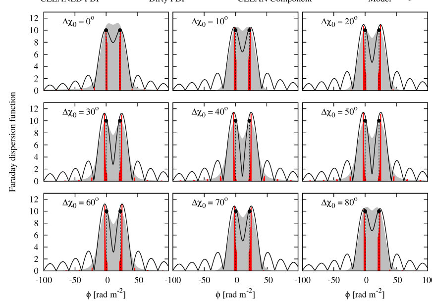
Figure 2: Faraday dispersion function (FDF) for $\Delta\chi_{0}=$ 0 - 80 degree, $A_{2}/A_{1}=1.0$, and $\Delta\phi=22.26$ rad m^-2 (1.0 FWHM) for the case with ASKAP. The black dot-dashed and solid lines represent the model and reconstructed FDFs, respectively. The shaded area in gray shows the cleaned FDF calculated by RM CLEAN algorithm. The red lines are the accumulated CLEAN components.

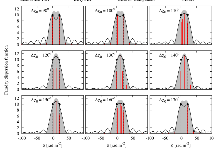
Figure 3: Same as Figure 2 but for $\Delta\chi_{0}=$ 90 - 170 degree.

In figures 2 and 3, we show the results of Faraday tomography and RM CLEAN for the cases with different $\Delta\chi_{0}$, where $A_{2}/A_{1}=1.0$ and $\Delta\phi=22.26$ rad m^-2 (1.0 FWHM) for the case with ASKAP are fixed. The two components are correctly detected except for the cases with $110^{\circ}\leq\Delta\chi_{0}\leq 160^{\circ}$. In the cases with $110^{\circ}\leq\Delta\chi_{0}\leq 160^{\circ}$, the reconstructed FDF has a single peak around the mean Faraday depth of the two components and the CLEAN components includes false signal larger than the correct signals. This phenomenon was reported by Farnsworth et al. (2011) as RM ambiguity. One may think that the result should be symmetric with respect to $\Delta\chi_{0}=90^{\circ}$, that is, the result should depend only on the absolute value of the $\Delta\chi_{0}$. Actually, this is not the case and the asymmetry comes from the relative sign of $\Delta\chi_{0}$ and $\Delta\phi$.

Farnsworth et al. (2011) indicated that two sources with a close separation $\Delta\phi\lesssim$ 1.0 FWHM would be detected as a single, false source, which is actually confirmed with Figure 3. On the other hand, there has not been reported that false signals arise for the cases with $\Delta\phi$ sufficiently larger than the FWHM. In order to make clear the border of RM ambiguity, in the next subsection we study the cases with $\Delta\phi\gtrsim$ 1.0 FWHM and do not consider the cases with $\Delta\phi\ll$ 1.0 FWHM.

3.2 Separation between components, $\Delta\phi$

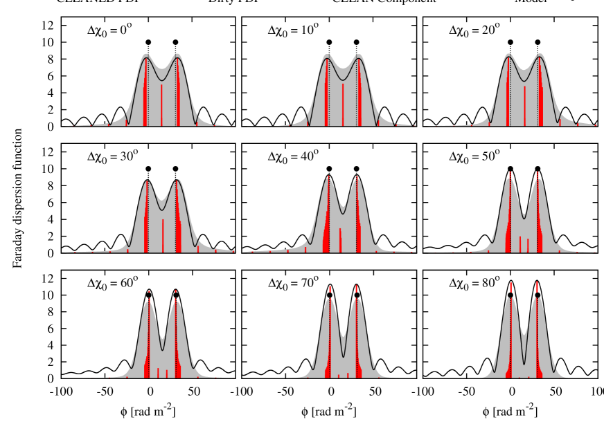
Figure 4: Faraday dispersion function (FDF) for $\Delta\chi_{0}=$ 0 - 80 degree, $A_{2}/A_{1}=1.0$, and $\Delta\phi=31.16$ rad m^-2 (1.4 FWHM) for the case with ASKAP. Descriptions of lines and colors are the same as Figure 2.

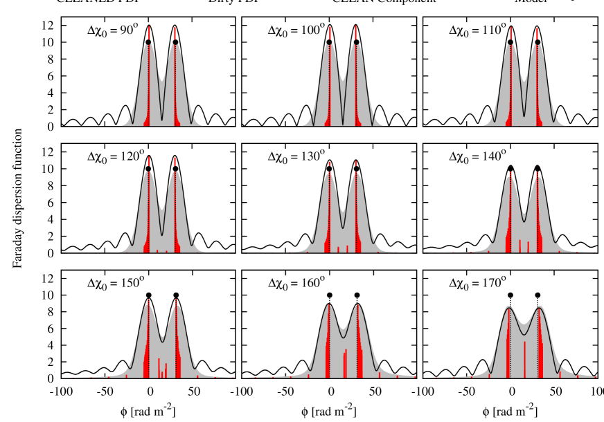
Figure 5: Same as Figure 4 but for $\Delta\chi_{0}=$ 90 - 170 degree.

Figures 4 and 5 show the FDFs for the cases with $\Delta\phi=1.4$ FWHM. Here, for quantification, we define the false signals to be CLEAN components arisen in Faraday depth from $\Delta\phi/4$ to $3\Delta\phi/4$ with an amplitude larger than half of that of the largest CLEAN component. In all cases, the reconstructed FDF and cleaned FDF have two peaks near the input Faraday depth and the CLEAN components located at the correct positions are dominant. However, false signals can be seen in the cases with $0\leq\Delta\chi_{0}\leq 20$ and $\Delta\chi_{0}=170$. Thus, false signals appear even for a source separation larger than the FWHM of the RMSF.

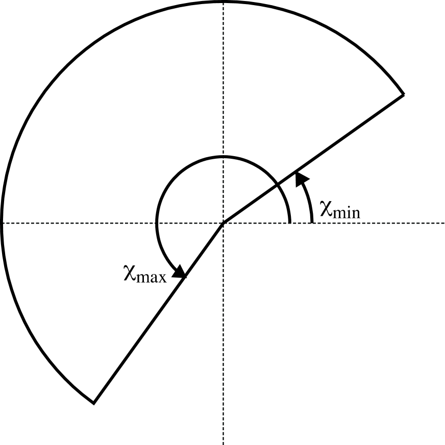
Figure 6: Definition of the pie display for rotation angles of light emitted by the second source ($k=2$). $\chi_{\rm max}=\Delta\phi\lambda^{2}_{\rm max}$ and $\chi_{\rm min}=\Delta\phi\lambda^{2}_{\rm min}$ are the rotation angles at the first source used in Figure 7 and 10.

To understand how large separation is needed to avoid false signals, we investigate false signals for the cases with various values of $\Delta\phi$, fixing the other parameters. For systematic displays, we show the rotation angles of light emitted by the second source ($k=2$) as a sector shaped with a thick line shown in Figure 6, where $\chi_{\rm max}=\Delta\phi\lambda^{2}_{\rm max}$ and $\chi_{\rm min}=\Delta\phi\lambda^{2}_{\rm min}$ are the rotation angles for $\lambda_{\rm max}$ and $\lambda_{\rm min}$ at the first source.

Figure 7 summarize the results for $\Delta\phi=1.0-1.7$ FWHM. The red sectors represent the range of $\Delta\chi_{0}$ where false signals appear in the CLEAN components. We find that false signals tend to appear when $\Delta\chi_{0}\sim(\Delta\phi\lambda^{2}_{\rm min}+\Delta\phi\lambda^{2}_{\rm max})/2$. This would be understandable because the resultant polarizations emitted from the two sources are similar each other in this case, and thus it is rather difficult to separate the both sources correctly. We also find that the range of $\chi_{0,1}$ which induces false signals does not become narrow monotonically as $\Delta\phi$ increases.

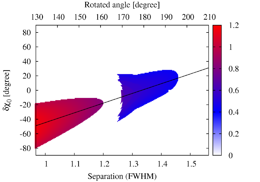
Figure 8: Amplitude of false signals in the CLEAN components. Colors show the amplitudes for different separations ($\Delta\phi$) and different intrinsic polarization angles ($\delta\chi_{0}$). Amplitude is shown as the ratio between amplitudes of the first and second largest CLEAN components, and false signals with the amplitude less than 0.5 are not shown. The black solid line represents the rotation angle of light at the first source with the wavelength $(\lambda^{2}_{\rm min}+\lambda^{2}_{\rm max})/2$ emitted by the second source ($k=2$).

Figure 8 shows the amplitude of the false signals for various $\Delta\phi$ and $\Delta\chi_{0}$, where we use $\delta\chi_{0}$, instead of $\Delta\chi_{0}$, defined as,

$$\delta\chi_{0}=\left\{\begin{array}[]{ll}\Delta\chi_{0}&{\rm for}\quad\Delta\chi_{0}\leq 90^{\circ}\\ \Delta\chi_{0}-180^{\circ}&{\rm for}\quad\Delta\chi_{0}>90^{\circ}.\end{array}\right.$$ (13)

We can see that the region in which we see false signals is along the black solid line, which is the track for the light satisfying $(\lambda^{2}_{\rm min}+\lambda^{2}_{\rm max})/2$ emitted by the second source, i.e. false signals tend to appear when $\Delta\chi_{0}\sim(\Delta\phi\lambda^{2}_{\rm min}+\Delta\phi\lambda^{2}_{\rm max})/2$ as seen in Figure 7. We can see that the false signals are larger than the correct signals for $\Delta\phi<1.1~{}{\rm FWHM}$. The false signals become weaker for larger $\Delta\phi$ but continue to appear up to $\Delta\phi=1.45~{}{\rm FWHM}$, while there is a gap in $\Delta\phi=1.2-1.25~{}{\rm FWHM}$. The separation corresponding to the gap is equal to the location of the second peak of the RMSF (Figure 1) whose amplitude is about 20% of that of the main peak. Thus, this gap is considered to be generated by the sidelobe, which enhances the other source and makes the detections easier, by accident.

3.3 Intensity ratio, $A_{2}/A_{1}$

We next investigate the dependence of false signals on the intensity ratio between the two sources, $A_{2}/A_{1}$. For each $A_{2}/A_{1}$, we validate the appearance of false signals in the case with $0^{\circ}\leq\Delta\chi_{0}\leq 180^{\circ}$ and $0.8\leq\Delta\phi\leq 1.5$ FWHM then pick up the worst case. The appearance of false signals can be classified into three types. Type (I) is that false signals appear for some intrinsic polarization angles and they are larger than the correct signals. Type (II) is that false signals appear for some intrinsic polarization angles and they are smaller than the correct signals. And type (III) is that there is no false signals for any intrinsic polarization angle.

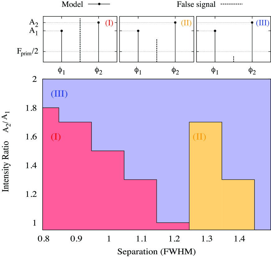
Figure 9: Appearance of RM ambiguity in lower panel. (I) False signals appear for some intrinsic polarization angles and they are larger than the correct signals with intensities $A_{1}$ and $A_{2}$. (II) False signals appear for some intrinsic polarization angles and they are smaller than the correct signals. (III) There is no false signals for any intrinsic polarization angle. In upper panels, we show the examples of type of False signals. False signals are defined as the CLEAN components arisen in Faraday depth from $\Delta\phi/4$ to $3\Delta\phi/4$ with an amplitude larger than half of that of the largest CLEAN component $F_{\rm prim}$.

Figure 9 shows the distribution of the three types. There is a tendency that larger $A_{2}/A_{1}$ reduces the generation of false signals and two sources can be successfully resolved even for a separation smaller than the FWHM of the RMSF if $A_{2}/A_{1}\gtrsim 1.8$. It is seen that false signals are serious when the two sources have comparable intensities and the separation is about the FWHM.

3.4 Frequency Coverage

Finally, we change frequency coverage. Figure 10 shows the results of the same analysis in Figure 7 but for the proposed bandwidth of SKA. We find that the results are very similar to the case of ASKAP. Thus, false signals are unavoidable regardless of the bandwidth, if we scaled $\phi$ separation by the FWHM of RMSF. We expect that false signals appear in the cases with a certain $\Delta\chi_{0}$ whenever $\Delta\phi$ is less than $\sim 1.5$ FWHM.

4 Summary and discussion

Faraday tomography combined with RM CLEAN is a powerful method to investigate the distribution of polarized sources along the LOS. However, in the presence of multiple sources, large false signals can appear in the middle of the correct signals in $\phi$ space. In this paper, we studied the condition of the appearance of false signals, focusing on the difference in the intrinsic polarization angles, the separation in $\phi$ space and the intensity ratio. We simulated the observations of ASKAP and SKA assuming two polarized sources and found that false signals can appear for a separation as large as 1.5 FWHM of the RMSF and the false signals exceed the correct signals for a separation smaller than 1.1 FWHM. The intensity ratio is also a important factor and large ratio tends to reduce the RM ambiguity. It should be noted that these results does not depend on the bandwidth of the telescope so that even future wide-band observation would suffer from RM ambiguity.

It should be noted that an absolute value of $\Delta\phi$ for which we see false signals is decreased as decreasing the FWHM. More specifically, false signals arise for the relative RM smaller than 22.26 rad/m² with ASKAP, but than 0.189 rad/m² with SKA. Therefore, false signals would become a minor issue in the SKA era while we study RMs of a few rad/m² or larger.

RM CLEAN has three parameters, the gain factor $\gamma$, threshold intensity, and maximum iteration. We also have studied the cases with different parameters, and found that larger gain factor tends to slightly increase the range of $\Delta\chi_{0}$ where false signals arise. On the other hand, threshold intensity and maximum iteration in this work are rather conservative values and the results were not changed significantly. Note that threshold intensity is usually referred to RMS noise level of the observations. Therefore, if we study polarization sources with less than mJy, the threshold intensity in this work could reach the RMS noise levels of ASKAP and SKA, and thus should increase the threshold. For such cases, we may need more careful arguments for the RM CLEAN parameters.

Finally, Stokes’ QU-fitting is another powerful method to probe cosmic magnetism with polarization observation (O’Sulivan et al., 2012; Ideguchi et al., 2013). In this method, fitting of polarization spectrum is performed assuming a model of source distribution with free parameters. Combination of QU-fitting and Faraday tomography would be effective to identify and avoid RM ambiguity, and detect correct polarized sources. This possibility will be pursued elsewhere in near future.

Table 1: Frequency Coverage and the FWHM.

Project	Frequency	$\lambda^{2}_{\rm max}$	$\lambda^{2}_{\rm min}$	FWHM
	GHz	m2	m2	rad/m2
ASKAP	$0.7-1.8$	1.83 $\times 10^{-1}$	2.76 $\times 10^{-2}$	22.26
SKA	$0.1-10$	1.83 $\times 10^{1}$	9.0 $\times 10^{-4}$	0.189

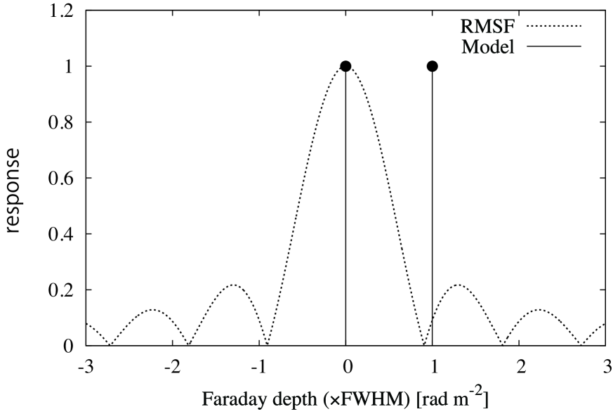
Figure 1: The rotation measure spread function (RMSF) and an example of the model of Faraday dispersion function which is composed of 2 point sources.

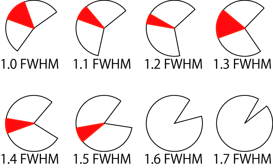
Figure 7: Appearance of false signals. The black sectors are the same as Figure 6 but for different FWHMs. The red sectors represent the range of $\Delta\chi_{0}$ where false signals appear in the CLEAN components.

Figure 10: Same as Figure 7 but for the case of SKA.

References

- Akahori & Ryu (2010) Akahori, T., & Ryu, D. 2010, ApJ, 723, 476
- Akahori & Ryu (2011) Akahori, T., & Ryu, D. 2011, ApJ, 738,134
- Akahori et al. (2012) Akahori, T., Kumazaki, K., Takahashi, K. & Ryu, D. 2012, submitted
- Andrecut et al. (2012) Andrecut, M., Stil, J. M., & Taylor, A. R. 2012, AJ, 143, 33
- Andrecut (2013) Andrecut, M. 2013, MNRAS, 430, L15
- Beck (2009) Beck, R. 2009, Rev. Mexicana Astron. Astrofis. (Serie de Conferencias), 36, 1
- Beck et al. (2012) Beck, R., Frick, P., Stepanov, R., & Sokoloff, D. 2012, A&A, 543, 113
- Bell et al. (2012) Bell, M. R., Oppermann, N., Crai, A., & Enßlin, T. A. 2013, A&A, 551, L7
- Brentjens & de Bruyn (2005) Brentjens, M. A., & de Bruyn, A. G. 2005, A&A, 441, 1217
- Brentjens (2011) Brentjens, M. A. 2011, A&A, 526, 9
- Burn (1966) Burn, B. J. 1966, MNRAS, 133, 67
- Farnsworth et al. (2011) Farnsworth, D., Rudnick, L., & Brown, S. AJ, 141, 28
- Fletcher et al. (2011) Fletcher, A., Beck, R., Shukurov, A., Berkhuijsen, E. M., & Hollerou, C. 2011, MNRAS, 412, 2396
- Frick et al. (2011) Frick, P., Sokoloff, D., Stepanov, R., & Beck, R. 2011, MNRAS, 414, 2540
- Fujita & Ohira (2013) Fujita, Y., & Ohira, Y., 2013, MNRAS, 421, 1434
- Gaensler et al. (2005) Gaensler, B. M., Haverkorn, M., Staveley-Smith, L., Dickey, J. M., McClure-Griffiths N. M., Dickel, J. R., & Wolleben, M., 2005, Science, 307, 1610
- Heald (2009) Heald, G. 2009, in IAU Symposium Vol. 259 of IAU Symposium, pp 591-602
- Heald (2009) Heald, G., Braun, R., & Edmonds, R. 2009, A&A, 503, 409
- Högbom (1974) Högbom, J. A. 1974, A&AS, 15, 417
- Iacobelli (2013) Iacobelli, M., Haverkorn, M., & Katgert, P. 2013, A&A, 549, 56
- Ideguchi et al. (2013) Ideguchi, S., Takahashi, K., Akahori, T., Kumazaki, K., & Ryu, D. 2013, PASJ in press (arXiv:1308.5696)
- Machida et al. (2013) Machida, M., Nakamura, K., Kudo, T., Akahori, T., Sofue, Y., & Matsumoto, R., 2012, ApJ, 764, 81
- Noutsos (2012) Noutsos, A. 2012, Space Science Reviews, 166, 1–4
- Neronov & Vovk (2010) Neronov, A., & Vovk, I. 2010, Science, 328, 73
- O’Sulivan et al. (2012) O’Sulivan, S. P., Brown, S., Robishaw, T., Schnitzeler, D. H. F. M., McClure-Griffiths, N. M., Feain, I. J., Taylor, A. R., Gaensler, B. M., Landecker, T. L., Harvey-Smith, L., & Carretti, E. 2012, MNRAS, 421, 3300
- Schnitzeler et al. (2009) Schnitzeler, D. H. F. M., Katgert, P., & de Bruyn, A. G. 2009, A&A, 494, 611
- Takahashi et al. (2012) Takahashi, K., Mori, M., Ichiki, K., & Inoue, S. 2012, ApJ, 4, L7
- Takahashi et al. (2013) Takahashi, K., Mori, M., Ichiki, K., Inoue, S., & Takami, H. 2013, ApJ, 771, L42
- Takami & Sato (2010) Takami, H., & Sato, K. 2010, ApJ, 724, 1456
- Takizawa (2008) Takizawa, M. 2008, ApJ, 687, 951
- Wolleben et al. (2010) Wolleben, M., Landecker, T. L., Hovey, G. J., Messing, R., Davison, O. S., House, N. L., Somaratne, K. H. M. S., & Tashev, I. 2010, AJ, 139, 1681