Surface Phase Transition in Anomalous Fluid in Nanoconfinement

Abstract

We explore by molecular dynamic simulations the thermodynamical behavior of an anomalous fluid confined inside rigid and flexible nanopores. The fluid is modeled by a two length scale potential. In the bulk this system exhibits the density and diffusion anomalous behavior observed in liquid water. We show that the anomalous fluid confined inside rigid and flexible nanopores forms layers. As the volume of the nanopore is decreased the rigid surface exhibits three consecutive first order phase transitions associated with the change in the number of layers. These phase transitions are not present for flexible confinement. Our results indicate that the nature of confinement is relevant for the properties of the confined liquid what suggests that confinement in carbon nanotubes should be quite different from confinement in biological channels.

I Introduction

Most liquids contract on cooling and diffuse faster as the density is decreased. This is not the case of the anomalous liquids in which the density exhibits a maximum at constant pressure and the diffusion coefficient increases under compression Chaplin (2013). These anomalous fluids include water Kell (1975); Angell et al. (1976); Prielmeier et al. (1987), Te Thurn and Ruska (1976), Ga, Bi Han (1984), Si Sauer and Borst (1967); Kennedy and Wheeler (1983), $Ge_{15}Te_{85}$ Tsuchiya (1991), liquid metals Cummings and Stell (1981) and graphite Togaya (1997). Computer simulations for silica Angell et al. (2000); Shell et al. (2002); Sharma et al. (2006), silicon Sastry and Angell (2003) and $BeF_{2}$ Angell et al. (2000) also show the presence of thermodynamic anomalies Prielmeier et al. (1987). In addition to the presence of a maximum of density in constant pressure, silica Sastry and Angell (2003); Shell et al. (2002); Sharma et al. (2006); Chen et al. (2006a), silicon Morishita (2005) and water Netz et al. (2001, 2002) exhibit a maximum in the diffusion coefficient at constant temperature.

Classical all-atom models such as SPC/E Berendsen et al. (1987), TIP4P-2005 Abascal and Vega (2005) and TIP5P Mahoney and Jorgensen (2000) for water, sW Stillinger and Weber (1985) for silicon or BKS van Beest et al. (1990) for silica have been employed to reproduce quantitatively these anomalous properties of these materials. However, coarse-grained potentials are an interesting tool able to identify what is the common structural property in these fluids that make them anomalous. The effective potentials derived in these coarse grained models are analytically more tractable and also computationally less expensive, what allow for studying a very large systems and complex mixtures. Several effective models have been proposed Jagla (1998); Xu et al. (2006); Yan et al. (2005); Xu et al. (2005); de Oliveira et al. (2006a); Camp (2005); Wilding and Magee (2002); Almarza et al. (2009); Fomin et al. (2008); Franzese et al. (2001); Franzese and Stanley (2007). They reproduce the thermodynamic, structural and dynamic anomalies present in water and in other anomalous liquids. The common ingredient in these potentials is that the particle-particle interaction is modeled through core-softened potentials formed by two length scales, one repulsive shoulder and an attractive well de Oliveira et al. (2006a, b); Jr et al. (2009); da Silva et al. (2010). These competition leads to the density and diffusion anomalies.

In addition to the bulk properties, nanoconfinement of anomalous liquids has been attracting attention not only due to its applications but also due to the new physics observed in these systems Malescio et al. (2005); Holt et al. (2006); Whitby et al. (2008). Fluids confined in carbon nanotube exhibit formation of layers, crystallization of the contact layer Cui et al. (2001); Jabbarzadeh et al. (2006) and a superflow not present in macroscopic confinement Jakobtorweihen et al. (2005); Chen et al. (2006b); Qin et al. (2011).

In the particular case of water confined in nanopores, the pore size has significant influence on the freezing and melting temperatures of water Erko et al. (2011); Deschamps et al. (2010); Jähnert et al. (2008); Morishige and Nobuoka (1997). The crystallization in these systems is not uniform and the confined ice shows different characteristics when compared with the bulk ice Kastelowitz et al. (2010). Hydrophobic Mao and Sinnot (2002); Ackerman et al. (2003); Qin et al. (2011); Khademi and Sahimi (2011) and hydrophilic Lee et al. (2012) confinements also induce different effects in the layering, density and flow of water.

Atomistic studies of nanoconfinement of water show another property: confined systems exhibit a phase transition not observed in the bulk system. SPC/E model confined between atomically smooth plates Giovambattista et al. (2009); Lombardo et al. (2009) and TIP4P water inside nanotubes Koga et al. (2001) shows a first order phase transition between a bilayer liquid (or ice) and a trilayer heterogeneous fluid. These studies, however, has been restricted to rigid nanotubes. The flexibility of the nanochannel Jakobtorweihen et al. (2005); Chen et al. (2006b) and of biological ionic channels Noskov et al. (2004); Beckstein and Sansom (2004); Allen et al. (2004); Chiu et al. (1991) show properties different from the behavior observed in confinement by rigid walls. These studies, however, do not highlight the physical reason behind the differences between rigid and flexible confinement.

Acknowledging that coarse graining potentials would be a suitable tool to test how the flexibility would affect the properties of confined anomalous liquids. Recently it was shown that the density and diffusion anomalies disappears as the channel or nanopore become flexible Krott and Bordin (2013).

In this paper we explore the differences in the layering and in the surface phase transitions for anomalous fluids confined by both rigid and flexible nanotubes. We show that the surface crystallization observed in rigid carbon nanotubes should not be expected in flexibly biological channels. The fluid is modeled using a two length scale potential. This coarse grained potential exhibits the thermodynamic, dynamic and structural anomalous behavior observed in anomalous fluids in bulk de Oliveira et al. (2006a, b) and in confinement Krott and Barbosa (2013); Krott and Bordin (2013); Krott and Barbosa (2014); Bordin et al. (2012, 2013). The formation of layers and its relation with the first order phase transition are analyzed. The paper is organized as follows: in Sec. II we introduce the model and describe the methods and simulation details; the results are given in Sec. III; and in Sec. IV we present our conclusions.

II The Model and the Simulation Methodology

The fluid is modeled as spherical-symmetric particles, with diameter $\sigma$ and mass $m$. The particles interact through the three dimensional core-softened potential de Oliveira et al. (2006a)

$$\frac{U(r_{ij})}{\varepsilon}=4\left[\left(\frac{\sigma}{r_{ij}}\right)^{12}-\left(\frac{\sigma}{r_{ij}}\right)^{6}\right]+u_{0}{\rm{exp}}\left[-\frac{1}{c_{0}^{2}}\left(\frac{r_{ij}-r_{0}}{\sigma}\right)^{2}\right]$$ (1)

where $r_{ij}=|\vec{r}_{i}-\vec{r}_{j}|$ is the distance between two fluid particles $i$ and $j$. This potential has two contributions. The first parcel is the standard $12-6$ Lennard-Jones (LJ) potential Allen and Tildesley (1987) and the second term is a Gaussian centered at $r_{0}/\sigma=0.7$, with depth $u_{0}\varepsilon=5.0$ and width $c_{0}\sigma=1.0$. With these parameters, the equation 1 represents a two length scale potential, with one scale at $r_{ij}\approx 1.2\sigma$, where the force has a local minimum, and the other scale at $r_{ij}\approx 2\sigma$, where the fraction of imaginary modes has a local minimum de Oliveira et al. (2010), as shown in figure 1. The fluid-fluid interaction, equation (1), has a cutoff radius $r_{\rm cut}/\sigma=3.5$. Despite the mathematical simplicity of the model, this fluid exhibits the thermodynamic, dynamic and structural anomalies present in bulk water de Oliveira et al. (2006a, b) and a water-like behavior when confined between plates Krott and Barbosa (2013); Krott and Bordin (2013); Krott and Barbosa (2014) or inside hydrophobic nanotubes Bordin et al. (2012, 2013).

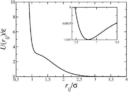
Figure 1: Interaction potential between anomalous fluid particles pair as function of their separation. Inset: zoom over the small attractive part of the interaction.

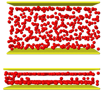
Figure 2: Snapshot of the simulation box for system for large (up) and narrow (down) nanopores.

The nanopore was modeled using two flat parallel walls, with fixed dimension $L\times L$, where $L=40\sigma$, separated by a distance $L_{z}$. In the figure 2 we show the snapshot of the system for two distinct configurations, one with a large $L_{z}$, where the fluid shows a bulk-like behavior, and the other a highly confined fluid. The fluid-wall interaction is purely repulsive, and was represented by the Weeks-Chandler-Andersen (WCA) Weeks et al. (1971) potential,

$$U^{\rm{WCA}}(z_{ij})=\left\{\begin{array}[]{ll}U_{{\rm{LJ}}}(z_{ij})-U_{{\rm{LJ}}}(z_{c})\;,\qquad z_{ij}\leq z_{c}\;,\\ 0\;,\qquad\qquad\qquad\qquad\quad z_{ij}>z_{c}\;.\end{array}\right.$$ (2)

Here, $U_{{\rm{LJ}}}$ is the standard $12-6$ LJ potential, included in the first term of equation (1), and $z_{c}=2^{1/6}\sigma$ is the cutoff for the WCA potential. Also, the term $z_{ij}$ measures the distance between the wall at $j$ position and the $z$-coordinate of the fluid particle $i$.

Two distinct scenarios were studied: rigid and flexible walls. In the first case, the nanopore walls positions were fixed and standard $NVT$ Molecular Dynamic simulations were performed. The temperature control was obtained with the Nosè-Hoover thermostat, with a coupling parameter $Q=2.0$. The pressure in the $z$ direction, $p_{z}$, was computed by the virial expression in the direction of the confinement ($z$) Zangi and Rice (2000), namely

$$p_{z}=\rho k_{b}T+\frac{1}{V}\langle W_{t}\rangle\;,$$ (3)

where

$$\langle W_{t}\rangle=-\sum_{1}^{N}\sum_{j>1}^{N}\frac{z_{ij}^{2}}{r_{ij}}\frac{\partial U}{\partial r}\;,$$

and $U(r_{ij})$ is the interaction potential between two particles separated by a distance $r_{ij}$, and $z_{ij}$ is the $z$-component of the distance.

In a second scenario flexible walls were studied. In this case, MD simulations were performed at constant number of particles and perpendicular pressure and temperature ($Np_{z}T$ ensemble). The pressure was fixed using the Lupkowski and van Smol method Lupowski and van Smol (1990). The walls had translational freedom in the $z$-direction, acting like a piston in the fluid, and a constant force controls the pressure applied in the confined direction. In this scenario, the resulting force in a fluid particle is given by

$$\vec{F}_{R}=-\vec{\nabla}U+\vec{F}_{iwA}(\vec{r}_{iA})+\vec{F}_{iwB}(\vec{r}_{iB})\;,$$ (4)

where $\vec{F}_{iwA(B)}$ indicates the interaction between the particle $i$ and the piston $A(B)$. Once the walls are non-rigid and time-dependent, we have to solve the equations of motion for $A$ and $B$,

$$m_{w}\vec{a}_{A}=p_{z}S_{w}\vec{n}_{A}-\sum_{i=1}^{N}\vec{F}_{iwA}(\vec{r}_{iA})$$ (5)

and

$$m_{w}\vec{a}_{B}=p_{z}S_{w}\vec{n}_{B}-\sum_{i=1}^{N}\vec{F}_{iwB}(\vec{r}_{iB})\;,$$ (6)

respectively, where $m_{w}$ is the piston mass, $p_{z}$ is the applied pressure in the system, $S_{w}$ is the piston area and $\vec{n}_{A}$ is an unitary vector in positive $z$-direction, while $\vec{n}_{B}$ is a negative unitary vector. Both pistons ($A$ and $B$) have mass $m_{w}=m$, width $\sigma$ and area equal to $S_{w}=L^{2}$.

For the rigid nanopore system, the temperature was varied from $k_{B}T=0.05$ to $k_{B}T=1.00$, and the plate separation from $L_{z}=4.00\sigma$ to $L_{z}=10.00\sigma$, while for systems with flexible nanopores the temperature was varied from $k_{B}T=0.10$ to $k_{B}T=1.00$, and the perpendicular pressure from $p_{z}\sigma^{3}/\epsilon=0.075$ to $p_{z}\sigma^{3}/\epsilon=6.00$. In both cases the simulations where performed with $N=1000$ particles. Standard periodic boundary conditions where applied in the non-confined directions. Five independent runs were performed to evaluate the properties of the confined fluid. Each individual simulation consists of $1\times 10^{6}$ equilibration steps and $3\times 10^{6}$ steps for production, with a time step $\delta t=0.0025$, in LJ units.

In order to define the fluid characteristics in contact with the nanopore walls, the structure of the fluid contact layer was analyzed using the radial distribution function $g_{||}(r_{xy})$, defined as

$$g_{\parallel}(r_{xy})\equiv\frac{1}{\rho^{2}V}\sum_{i\neq j}\delta(r-r_{ij})\left[\theta\left(\left|z_{i}-z_{j}\right|\right)-\theta\left(\left|z_{i}-z_{j}\right|-\delta z\right)\right].$$ (7)

where the Heaviside function $\theta(x)$ restricts the sum of particle pair in a slab of thickness $\delta z=1.0$ close to the wall.

The physical quantities in this paper are depict in LJ units Allen and Tildesley (1987),

$$r^{*}\equiv\frac{r}{\sigma}\;,\quad\rho^{*}\equiv\rho\sigma^{3}\;,\quad\mbox{and}\quad t^{*}\equiv t\left(\frac{\epsilon}{m\sigma^{2}}\right)^{1/2}\;,$$ (8)

for distance, density of particles and time , respectively, and

$$p^{*}\equiv\frac{p\sigma^{3}}{\epsilon}\quad\mbox{and}\quad T^{*}\equiv\frac{k_{B}T}{\epsilon}$$ (9)

for the pressure and temperature, respectively. Since all physical quantities are defined in reduced units in this paper, the ^∗ will be omitted in the results discussion.

In the simulations with flexible nanopores, the mean variation in the system size induced by the wall fluctuations are smaller than $2\%$. Data errors smaller than the data points are not shown.

III Results and Discussion

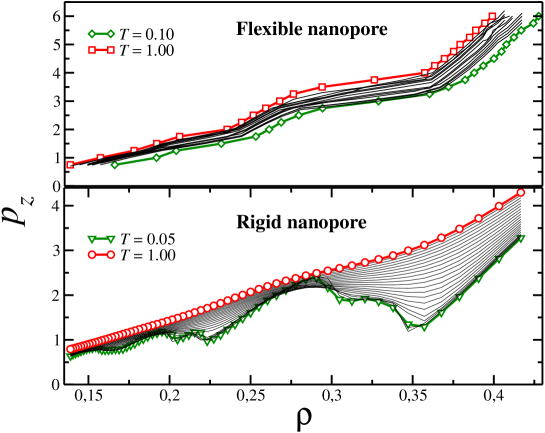
Figure 3: Pressure in the confined direction as function of the fluid density for flexible and rigid nanopores for several values of temperature. For simplicity, only the higher and lower value of $T$ for the isotherms is detached. A non-monotonic behavior was observed when the anomalous fluid is confined inside rigid nanopores. All the quantities are in reduced units.

In order to understand the thermodynamical properties of the anomalous fluid under confinement, the $p_{z}\times\rho$ phase diagram is analyzed for the cases with flexible or rigid nanopores. Figure 3 illustrates the pressure in the confined direction versus density phase diagram for various temperatures. For the flexible nanopores, all the isotherms show a monotonic behavior. This suggests that while the fluid between the plates changes its configuration between different layer arrangements the wall continuously and no phase transition at the wall is observed. For rigid nanopores, however, the pressure versus density is a monotonic function for isochores above $T_{c3}=0.45$. Below this temperature, a non-monotonic behavior is observed. The isotherms for $T<T_{ci}$ show a van der Waals loop, characteristic of a first order phase transition.

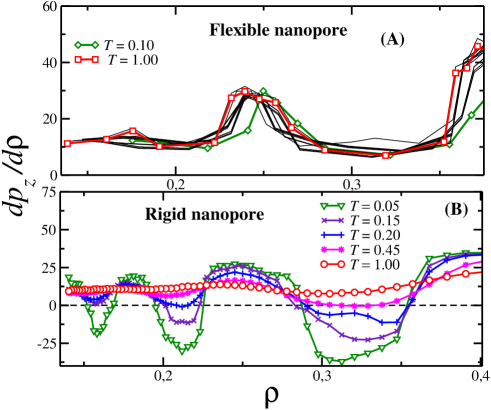
Figure 4: Pressure derivative versus density for different isotherms for (A) flexible or (B) rigid nanopores. In the rigid case, the inflection in $dp_{z}/d\rho=0$ indicates the presence of a first order phase transition.

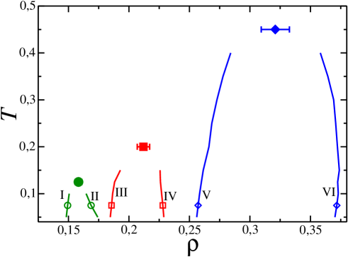
Figure 5: Temperature versus density phase diagram for the three coexistence regions and critical points: $(T_{c1}=0.125$, $p_{z,c1}=0.782$, $\rho_{c1}=0.1583)$ (sphere), $(T_{c2}=0.2$, $p_{z,c2}=1.1704$, $\rho_{c2}=0.212)$ (square) and $(T_{c3}=0.45$, $p_{z,c3}=2.235$, $\rho_{c3}=0.321)$ (diamond).The points I, II, III, IV, V and VI illustrate the coexistence densities at $T=0.075$ namely $\rho_{I}$, $\rho_{II}=$m $\rho_{III}$, $\rho_{IV}=$, $\rho_{V}=$ and $\rho_{VI}$.

For fluids confined inside flexible nanopores the pressure derivative with respect to density is always positive as illustrated by figure 4(A). For rigid confinement, the derivative is positive only for isochores $T>T_{c3}$. Below this threshold the function becomes negative for various densities as illustrated in figure 4(B). This figure identify three first order phase transitions. The densities of the coexistence phases can be obtained by Maxell construction. These three coexistence regions end in three critical points that can be located by computing the second derivative $d^{2}p/d\rho^{2}=0$. The coexisting phases and the three critical points are illustrated by symbols in the isochores in figure 5.

Before discussing the characteristics of the fluid and of the phase transition at the wall, we address the question of why the thermodynamical behavior of flexible nanopores should be different from the case of rigid nanopores. In the rigid case, the walls only contribute to the enthalpic part of the free energy while in the flexible case, the walls vibrations constantly shake the fluid particles near the wall, increasing also the entropic part of the free energy. While the minimization of the wall-particle and particle-particle energy leads to an ordered structure, the entropic contribution from the wall disrupts this organization. Therefore, only in the case of rigid walls an ordered structure at the wall should be expected. Consequently, since the central layers are not affected by the wall movement, we can understand the differences between the thermodynamical behavior of the confined fluid within rigid and flexible walls by analyzing the properties of the layers in contact with the walls. We will refer to this layer as contact layer.

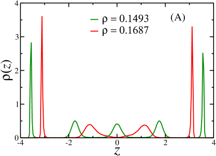
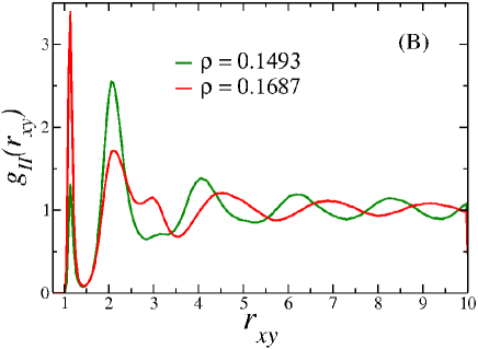
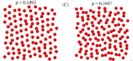
Figure 6: Density histogram (A), radial distribution function (B) and snapshots (C) for the anomalous fluid confined inside a rigid nanopore at $T=0.075$ and in the points I and II from figure 5.

Let us first analyze the fluid confined within rigid walls. The fluid within the walls form layers and as the density decreases, the number of layers increases. Figure 6(A) illustrates that for $T=0.075$ and pressure $p_{z}=0.762$ the system can have five or four layers, and the density would be $\rho_{I}=0.1493$ or $\rho_{II}=0.1687$ respectively. Figure 7(A) shows that the system can have four or three layers at the same temperature and perpendicular pressure if the density would be $\rho_{III}=0.18562$ or $\rho_{IV}=0.228$ respectively. Finally, the figure 8(A) has the the system with three or two layers depending if the density would be $\rho_{V}=0.2566$ or $\rho_{VI}=0.377$, respectively, with the same value of $p_{z}$. These three coexisting regions at $T=0.075$ are illustrated in the temperature versus density phase diagram of figure 5 as I, II, III, IV, V and VI.

The phase transition observed in the figure 5 can be associated with the change in the number of layers. In order to explore the idea that this transition is also associated with changes in the structure of the contact layer, the radial distribution function $g_{\parallel}(r_{xy})$ of the contact layer was computed. Figure 6(B) indicates that for $T=0.075$, $p_{z}=0.762$ and the densities $\rho_{I}$ or $\rho_{II}$ the contact layers exhibit two distinct structures. The high peak in the second length scale for the $g_{\parallel}(r_{xy})$ of $\rho_{I}=0.1493$ and the fact that between the two first peaks the radial distribution function is not equal to zero indicates that this layers is in a liquid-crystal like state. The $g_{\parallel}(r_{xy})$ for the density $\rho_{II}=0.1687$ shows a very structured liquid as well. It has a higher first peak when compared with the peak in the case $\rho_{I}$. The $\rho_{II}$ also has a displacement in the subsequent peaks what suggests an additional length scale in the arrangements of the particles. These two distinct particle arrangement are illustrated in the snapshots of the contact layer shown in figure 6(C). These pictures confirm the two structures predicted by the radial distribution function. The dimeric arrangement corresponds to the increase in the first peak of the $g_{\parallel}(r_{xy})$ for $\rho_{II}$ while the displacement of of the other peaks represent the second length. The systems exhibits a first-order phase transition from liquid-crystal-like to a dimeric structured liquid in the contact layer.

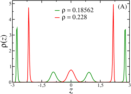
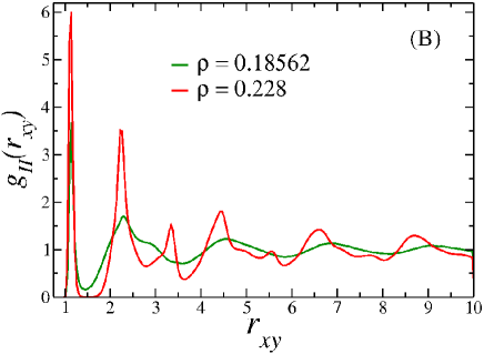
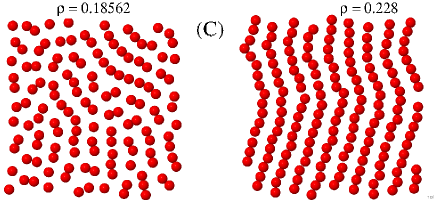
Figure 7: Density histogram (A), radial distribution function (B) and snapshots (C) for the anomalous fluid confined inside a rigid nanopore at $T=0.075$ and in the points III and IV from figure 5.

The $g_{\parallel}(r_{xy})$ for the densities $\rho_{III}=0.18562$ and $\rho_{IV}=0.228$, associated with the four to three layers in figure 7(A) respectively, are shown in figure 7(B). As the density changes from $\rho_{II}$ to $\rho_{III}$ the dimeric system becomes continuously more structured. As the density increases further, at $\rho_{IV}$ the system changes discontinuously to an ordered solid structure. As the snapshots in the figure 7(C) indicates, the dimers observed in figure 6(C) are now forming disordered lines in the density $\rho_{III}$. For the higher density $\rho_{IV}$ the line are completely arranged in a ordered structure. This indicates that the presence of a second first order transition from a structured liquid phase to a solid phase.

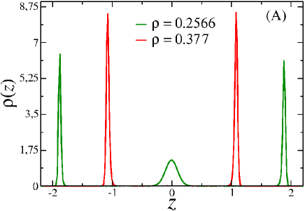
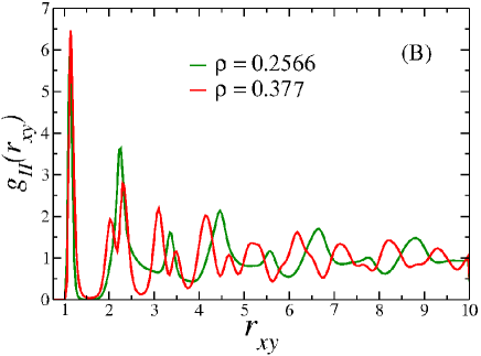
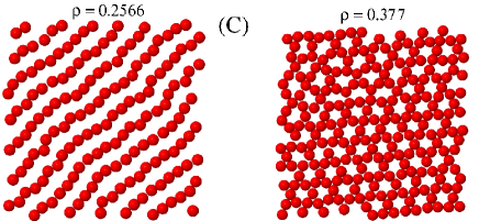
Figure 8: Density histogram (A), radial distribution function (B) and snapshots (C) for the anomalous fluid confined inside a rigid nanopore at $T=0.075$ and in the points V and VI from figure 5.

The radial distribution functions for densities $\rho_{V}=0.2566$ and $\rho_{VI}=0.377$ illustrated in figure 8(B) show a coexistence of two different highly ordered solid-like structures in the contact layer. Analysis using the snapshot of the figure 8(C) shows that for $\rho_{V}$ the particles form line that can be in different orientations. More important than this, the snapshots shows a structural transition from the lined conformation to a honeycomb structure. This surprising result shows that the third van der Waals loop corresponds to a solid-solid phase transition in the contact layer.

The three phase transitions at the surface are represented by the density jumps in the temperature versus density phase transition in figure 5 and by the van der Waals loops in figure 3 showing that the instabilities signalized in these graphs are related to phase transitions at the fluid wall interface. The transition between two solid or solid-like phases usually imply a change in the order parameter symmetry and, therefore, can not be modeled by a van der Waals theory. However, Daanoun, Tejero and Baus showed that the van der Waals theory can be extended to solid-solid transitions Daanoun et al. (1994) in some special cases. In this context, a number of solid-solid first-order phase transitions ending in critical points where found Bolhuis et al. (1994); Bolhuis and Frenkel (1997); Dijkstra (2002); Löwen (1997); Denton and Löwen (1997); Marcus and Rice (1997), particularly in 2D systems in which the particles interact through a two length scales potential Jagla (1998); Dudalov et al. (2013); Young and Alder (1977). Therefore, since the contact layer is a kind of 2D system, our model falls in the category and is not surprising that the surface would exhibit a solid-solid phase transition.

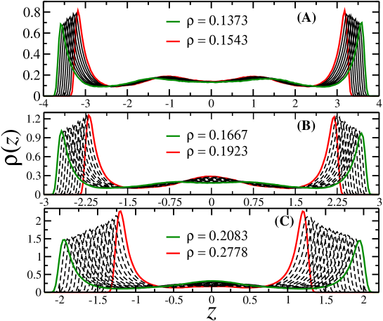
Figure 9: Density histogram for the anomalous fluid confined inside a rigid nanopore at temperatures above the critical point, $T=1.0$.

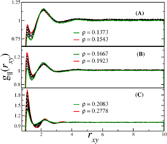
Figure 10: $g_{\parallel}(r_{xy})$ for the anomalous fluid confined inside a rigid nanopore at temperatures above the critical point, $T=1.0$.

For temperatures above the critical region the number of layers of the anomalous fluid confined inside a rigid nanopore does not change significantly. Figures 9(A), (B) and (C) illustrates the density across the nanopore for various plates separation, showing two contact layers and an uniform distribution inside the pore. The radial distribution function of the contact layer, presented in figure 10(A), (B) and (C), shows a fluid like behavior for all densities. In this way, at high temperatures the layers transition does not occur and the structure of the contact layer do not change, and none phase transition is observed.

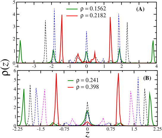
Figure 11: Density histogram (left - figures A and B) and $g_{\parallel}(r_{xy})$ (right - figures C and D) for the anomalous fluid confined inside a flexible nanopore at a low temperature, $T=0.10$

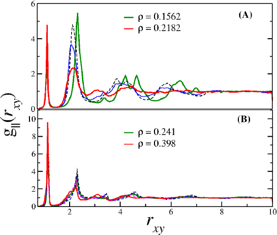
Figure 12: $g_{\parallel}(r_{xy})$ (right - figures C and D) for the anomalous fluid confined inside a flexible nanopore at a low temperature, $T=0.10$.

Next, we analyze the behavior of the anomalous fluid inside a flexible nanopore. Figure 11(A) and (B) shows the number of layers for different densities at $T=0.10$. As the density is increased the number of layers decrease from five to two layers. The nanopore flexibility leads also to a distinct behavior in the contact layer structure, which is strongly affected by the walls movement. Figure 12(A) and (B) illustrates the radial distribution function of the contact layer for various densities. In all the cases the $g_{\parallel}(r_{xy})$ shows a distinct signature of amorphous phase. This observation is supported by the snapshot shown in figure 13. The system exhibits a disordered structure similar to the amorphous phase. No phase transition is present as already indicated by the figure 4(A).

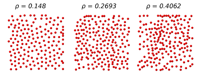
Figure 13: Contact layer snapshots in the flexible nanopore case. In all cases, a fluid-like structure was observed.

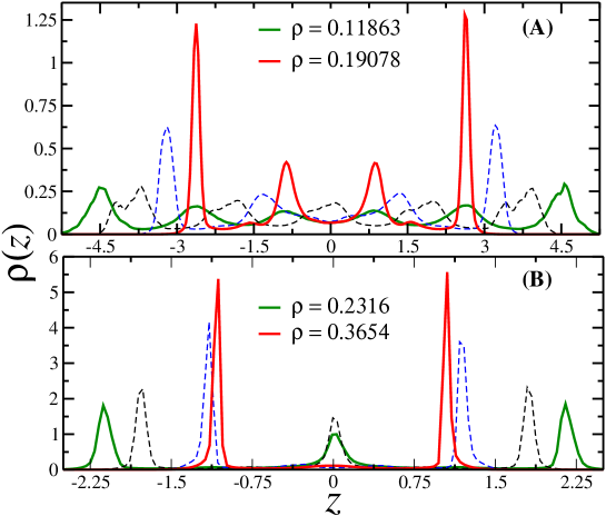
Figure 14: Density histogram for the anomalous fluid confined inside a flexible nanopore at a elevated temperature, $T=1.0$.

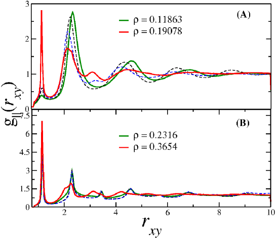
Figure 15: $g_{\parallel}(r_{xy})$ for the anomalous fluid confined inside a flexible nanopore at a elevated temperature, $T=1.0$.

Is important to point that the wall flexibility, despite maintaining the contact layer in a disordered structure, make more difficult to destroy the central layers at higher temperatures. At right temperatures, as $T=1.0$, and small density the system shows a bulk-like density profile, as shown in figure 14(A). But, for slightly higher densities, layering of the fluid is restored as illustrated in figure 14(B). This behavior is distinct from the rigid nanopore case in which for any density at high temperatures the layering is lost. Due to the wall oscillations the fluid particles can assume in the $z$-direction a position that minimizes the energy. And this small oscillation, compared with fixed walls, leads to the layering even for high temperatures, as shown in figure 14(A) and (B). This order in the middle layers at high temperatures does not affect the contact layer. Figure 15(A) and (B) shows that the the radial distribution function of the contact layer is similar to the amorphous phase.

IV Conclusion

We have studied the thermodynamical behavior and the surface phase transition of a anomalous fluid confined inside rigid and flexible nanopores. Our results show that the fluid behavior is strongly affected by the confinement properties. In the rigid nanopore scenario, the $p_{z}\times\rho$ phase diagram shows the presence of three first order phase transitions related with structural phase transitions at the contact layer. Due the walls fluctuations in the flexible nanopore case, no surface phase transition is observed in the case of non rigid walls. Our results indicates that the thermodynamic behavior of anomalous fluids such as water obtained for rigid carbon nanotubes and solid state nanopores can not be extrapolated to more flexible walls such as the surface present in biological systems.

V Acknowledgments

JRB would like to thanks Prof. A. Diehl from UFPel for the discussions. We thanks the Brazilian agencies CNPq, INCT-FCx, and Capes for the finantial support. We also thanks to CEFIC - Centro de Física Computacional of Physics Institute at UFRGS and the TSSC - Grupo de Teoria e Simulação em Sistemas Complexos at UFPel for the computer clusters.

References

- Chaplin (2013) M. Chaplin, “Sixty-nine anomalies of water,” http://www.lsbu.ac.uk/water/anmlies.html (2013).
- Kell (1975) G. S. Kell, J. Chem. Eng. Data 20, 97 (1975).
- Angell et al. (1976) C. A. Angell, E. D. Finch, and P. Bach, J. Chem. Phys. 65, 3065 (1976).
- Prielmeier et al. (1987) F. X. Prielmeier, E. W. Lang, R. J. Speedy, and H.-D. Lüdemann, Phys. Rev. Lett. 59, 1128 (1987).
- Thurn and Ruska (1976) H. Thurn and J. Ruska, J. Non-Cryst. Solids 22, 331 (1976).
- Han (1984) Handbook of Chemistry and Physics, 65th ed. (CRC Press, Boca Raton, Florida, 1984).
- Sauer and Borst (1967) G. E. Sauer and L. B. Borst, Science 158, 1567 (1967).
- Kennedy and Wheeler (1983) S. J. Kennedy and J. C. Wheeler, J. Chem. Phys. 78, 1523 (1983).
- Tsuchiya (1991) T. Tsuchiya, J. Phys. Soc. Jpn. 60, 227 (1991).
- Cummings and Stell (1981) P. T. Cummings and G. Stell, Mol. Phys. 43, 1267 (1981).
- Togaya (1997) M. Togaya, Phys. Rev. Lett. 79, 2474 (1997).
- Angell et al. (2000) C. A. Angell, R. D. Bressel, M. Hemmatti, E. J. Sare, and J. C. Tucker, Phys. Chem. Chem. Phys. 2, 1559 (2000).
- Shell et al. (2002) M. S. Shell, P. G. Debenedetti, and A. Z. Panagiotopoulos, Phys. Rev. E 66, 011202 (2002).
- Sharma et al. (2006) R. Sharma, S. N. Chakraborty, and C. Chakravarty, J. Chem. Phys. 125, 204501 (2006).
- Sastry and Angell (2003) S. Sastry and C. A. Angell, Nature Mater. 2, 739 (2003).
- Chen et al. (2006a) S.-H. Chen, F. Mallamace, C.-Y. Mou, M. Broccio, C. Corsaro, A. Faraone, and L. Liu, Proc. Natl. Acad. Sci. USA 103, 12974 (2006a).
- Morishita (2005) T. Morishita, Phys. Rev. E 72, 021201 (2005).
- Netz et al. (2001) P. A. Netz, F. W. Starr, H. E. Stanley, and M. C. Barbosa, J. Chem. Phys. 115, 344 (2001).
- Netz et al. (2002) P. A. Netz, F. W. Starr, M. C. Barbosa, and H. E. Stanley, Physica A 314, 470 (2002).
- Berendsen et al. (1987) H. J. C. Berendsen, J. R. Grigera, and T. P. Straatsma, J. Phys. Chem. 91, 6269 (1987).
- Abascal and Vega (2005) J. L. F. Abascal and C. Vega, J. Chem. Phys. 123, 234505 (2005).
- Mahoney and Jorgensen (2000) M. W. Mahoney and W. L. Jorgensen, J. Chem. Phys. 112, 8910 (2000).
- Stillinger and Weber (1985) F. H. Stillinger and T. A. Weber, Phs. Rev. B 31, 5262 (1985).
- van Beest et al. (1990) B. van Beest, G. Kramer, and R. van Santen, Phs. Rev. Lett. 64, 1955 (1990).
- Jagla (1998) E. A. Jagla, Phys. Rev. E 58, 1478 (1998).
- Xu et al. (2006) L. Xu, S. Buldyrev, C. A. Angell, and H. E. Stanley, Phys. Rev. E 74, 031108 (2006).
- Yan et al. (2005) Z. Yan, S. V. Buldyrev, N. Giovambattista, and H. E. Stanley, Phys. Rev. Lett. 95, 130604 (2005).
- Xu et al. (2005) L. Xu, P. Kumar, S. V. Buldyrev, S.-H. Chen, P. Poole, F. Sciortino, and H. E. Stanley, Proc. Natl. Acad. Sci. U.S.A. 102, 16558 (2005).
- de Oliveira et al. (2006a) A. B. de Oliveira, P. A. Netz, T. Colla, and M. C. Barbosa, J. Chem. Phys. 124, 084505 (2006a).
- Camp (2005) P. Camp, Phys. Rev. E 71, 031507 (2005).
- Wilding and Magee (2002) N. B. Wilding and J. E. Magee, Phys. Rev. E 66, 031509 (2002).
- Almarza et al. (2009) N. G. Almarza, J. A. Capitan, J. A. Cuesta, and E. Lomba, J. Chem. Phys 131, 124506 (2009).
- Fomin et al. (2008) D. Y. Fomin, , N. V. Gribova, V. N. Ryzhov, S. M. Stishov, and D. Frenkel, J. Chem. Phys 129, 064512 (2008).
- Franzese et al. (2001) G. Franzese, G. Malescio, A. Skibinsky, S. V. Buldyrev, and H. E. Stanley, Nature (London) 409, 692 (2001).
- Franzese and Stanley (2007) G. Franzese and H. E. Stanley, J. Phys.: Cond. Matter 19, 205126 (2007).
- de Oliveira et al. (2006b) A. B. de Oliveira, P. A. Netz, T. Colla, and M. C. Barbosa, J. Chem. Phys. 125, 124503 (2006b).
- Jr et al. (2009) N. M. Barraz Jr, E. Salcedo, and M. C. Barbosa, J. Chem. Phys. 131, 094504 (2009).
- da Silva et al. (2010) J. N. da Silva, E. Salcedo, A. B. de Oliveira, and M. C. Barbosa, J. Chem. Phys. 133, 244506 (2010).
- Malescio et al. (2005) G. Malescio, G. Franzese, A. Skibinsky, S. V. Buldyrev, and H. E. Stanley, Phys. Rev. E 71, 061504 (2005).
- Holt et al. (2006) J. K. Holt, H. G. Park, Y. M. Wang, M. Stadermann, A. B. Artyukhin, C. P. Grigoropulos, A. Noy, and O. Bakajin, Science 312, 1034 (2006).
- Whitby et al. (2008) M. Whitby, L. Cagnon, and M. T. ans N. Quirke, Nanoletters 8, 2632 (2008).
- Cui et al. (2001) S. T. Cui, P. T. Cummings, and H. D. Cochran, J. Chem. Phys. 114, 7189 (2001).
- Jabbarzadeh et al. (2006) A. Jabbarzadeh, P. Harrowell, and R. I. Tanner, J. Chem. Phys. 125, 034703 (2006).
- Jakobtorweihen et al. (2005) S. Jakobtorweihen, M. G. Verbeek, C. P. Lowe, . F. J. Keil, and B. Smit, Phys. Rev. Lett. 95, 044501 (2005).
- Chen et al. (2006b) H. Chen, J. K. Johnson, and D. S. Sholl, J. Phys. Chem. B Lett. 110, 1971 (2006b).
- Qin et al. (2011) X. Qin, Q. Yuan, Y. Zhao, S. Xie, and Z. Liu, Nanoletters 11, 2173 (2011).
- Erko et al. (2011) M. Erko, N. Cade, A. G. Michette, G. H. Findenegg, and O. Paris, Phys. Rev. B 84, 104205 (2011).
- Deschamps et al. (2010) J. Deschamps, F. Audonnet, N. Brodie-Linder, M. Schoeffel, and C. Alba-Simionesco, Phys. Chem. Chem. Phys. 12, 1440 (2010).
- Jähnert et al. (2008) S. Jähnert, F. V. Chávez, G. E. Schaumann, A. Schreiber, M. Schönhoff, and G. H. Findenegg, Phys. Chem. Chem. Phys. 10, 6039 (2008).
- Morishige and Nobuoka (1997) K. Morishige and K. Nobuoka, J. Chem. Phys. 107, 6965 (1997).
- Kastelowitz et al. (2010) N. Kastelowitz, J. C. Johnston, and V. Molinero, J. Chem. Phys. 132, 124511 (2010).
- Mao and Sinnot (2002) Z. Mao and S. B. Sinnot, Phys. Rev. Lett. 89, 278301 (2002).
- Ackerman et al. (2003) D. M. Ackerman, A. I. Skoulidas, D. S. Sholl, and J. K. Johnson, Mol. Simul. 29, 677 (2003).
- Khademi and Sahimi (2011) M. Khademi and M. Sahimi, J. Chem. Phys 135, 204509 (2011).
- Lee et al. (2012) K. P. Lee, H. Leese, and D. Mattia, Nanoscale 4, 2621 (2012).
- Giovambattista et al. (2009) N. Giovambattista, P. J. Rossky, and P. G. Debenedetti, Phys. Rev. Lett. 102, 050603 (2009).
- Lombardo et al. (2009) T. G. Lombardo, P. J. Rossky, and P. G. Debenedetti, Faraday Discuss. 141, 359 (2009).
- Koga et al. (2001) K. Koga, G. T. Gao, H. Tanaka, and X. C. Zeng, Nature 412, 802 (2001).
- Noskov et al. (2004) S. Y. Noskov, S. Berneche, and B. Roux, Nature 431, 830 (2004).
- Beckstein and Sansom (2004) O. Beckstein and M. S. P. Sansom, Phys. Biol. 1, 42 (2004).
- Allen et al. (2004) T. W. Allen, O. S. Andersen, and B. Roux, J. Gen. Physiol. 124, 679 (2004).
- Chiu et al. (1991) S.-W. Chiu, E. Jakobsson, S. Subramahiam, and J. A. McCammon, Biophys. J. 60, 273 (1991).
- Krott and Bordin (2013) L. Krott and J. R. Bordin, J. Chem. Phys. 139, 154502 (2013).
- Krott and Barbosa (2013) L. Krott and M. C. Barbosa, J. Chem. Phys. 138, 084505 (2013).
- Krott and Barbosa (2014) L. Krott and M. C. Barbosa, Phys. Rev. E 89, 012110 (2014).
- Bordin et al. (2012) J. R. Bordin, A. B. de Oliveira, A. Diehl, and M. C. Barbosa, J. Chem. Phys 137, 084504 (2012).
- Bordin et al. (2013) J. R. Bordin, A. Diehl, and M. C. Barbosa, J. Phys. Chem. B 117, 7047 (2013).
- Allen and Tildesley (1987) P. Allen and D. J. Tildesley, Computer Simulation of Liquids (Oxford University Press, Oxford, 1987).
- de Oliveira et al. (2010) A. B. de Oliveira, E. Salcedo, C. Chakravarty, and M. C. Barbosa, J. Chem. Phys. 132, 234509 (2010).
- Weeks et al. (1971) J. D. Weeks, D. Chandler, and H. C. Andersen, J. Chem. Phys. 54, 5237 (1971).
- Zangi and Rice (2000) R. Zangi and A. Rice, Phys. Rev. E 61, 660 (2000).
- Lupowski and van Smol (1990) M. Lupowski and F. van Smol, J. Chem. Phys. 93, 737 (1990).
- Daanoun et al. (1994) A. Daanoun, C. F. Tejero, and M. Baus, Phys. Rev. E 40, 2913 (1994).
- Bolhuis et al. (1994) P. Bolhuis, M. Hagen, and D. Frenkel, Phys. Rev. E 40, 4880 (1994).
- Bolhuis and Frenkel (1997) P. Bolhuis and D. Frenkel, J. Phys.: Cond. Matt. 9, 381 (1997).
- Dijkstra (2002) M. Dijkstra, Phys. Rev. E 66, 021402 (2002).
- Löwen (1997) H. Löwen, Physica A 235, 129 (1997).
- Denton and Löwen (1997) A. R. Denton and H. Löwen, J. Phys.: Condens. Matter 9, L1 (1997).
- Marcus and Rice (1997) A. H. Marcus and S. A. Rice, Phys. Rev. E 55, 637 (1997).
- Dudalov et al. (2013) D. Dudalov, Y. D. Fomin, E. Tsiok, and V. Ryzhov, arXiv:1311.7534v1 (2013).
- Young and Alder (1977) D. A. Young and B. J. Alder, Phys. Rev. Lett. 38, 1213 (1977).