How Does Latent Semantic Analysis Work? A Visualisation Approach

Abstract

By using a small example, an analogy to photographic compression, and a simple visualization using heatmaps, we show that latent semantic analysis (LSA) is able to extract what appears to be semantic meaning of words from a set of documents by blurring the distinctions between the words.

Keywords:

Latent Semantic Analysis, Singular Value Decomposition, Artificial Intelligence, Visualization

1 Introduction

Latent Semantic Analysis (LSA) was patented in 1988 (US Patent 4,839,853) and is a widely used technique in natural language processing for analyzing relationships between a set of documents and the words they contain. The literature on LSA is extensive, see, for example, the book-length collection Landuaer et al. (2011) and the many references therein. Among this literature are a number of excellent decriptions of the mathematics of LSA such as Deerwater et al. (1990), Berry et al. (1995) and Martin and Berry (2011).

Despite the existence of these excellent mathematical accounts of how LSA works, it is not widely understood. For example, recently Tunkelang (2008), discussed three alternative hypothesis but reached no conclusions. We suspect the reason for this is that to understand how LSA works, substantial knowledge of linear algebra and matrix computations is required in general, and of singular value decomposition (SVD) in particular, on the level provided in such textbooks as Meyer (2000, Sec. 5.12), Watkins (2002, Ch. 4) or Gentle (2007, Sect. 7.7) among many others. To those without such knowledge the discussion of the use of singular values or eigenvalues (for details of the exact nature of the relationship between singular values and eigenvalues see Meyer (2000) p. 555) and their corresponding eigenvectors in LSA is simply incomprehensible. It is our hope that by using a visualisation approach in this short note the understanding of how LSA works (at least at the intuitive level) will become available to a much wider audience, particularly to users of LSA with minimal mathematical backgrounds.

In this note we have used the words eigenvalue and eigenector, understanding that they carry little or no meaning to a non-mathematical reader, simply because they are standard terms.

The remainder of the note only contains two sections; Section (2) presents an example while Section (3) contains our conclusions.

2 Example

Document	Title
c1:	Human machine interface for ABC computer applications
c2:	A survey of user opinion of computer system response times
c3:	The EPS user interface management system
c4:	System and human system engineering testing of EPS
c5:	Relation of user perceived response time to error measurement
m1:	The generation of random, binary, ordered trees
m2:	The intersection graph of paths in trees
m3:	Graph minors IV: Width of trees and well-quasi-ordering
m4	Graph minors: A survey

Document	c1	c2	c3	c4	c5	m1	m2	m3	m4
Word
human	1	0	0	1	0	0	0	0	0
interface	1	0	1	0	0	0	0	0	0
computer	1	1	0	0	0	0	0	0	0
user	0	1	1	0	1	0	0	0	0
system	0	1	1	2	0	0	0	0	0
response	0	1	0	0	1	0	0	0	0
time	0	1	0	0	1	0	0	0	0
EPS	0	0	1	1	0	0	0	0	0
survey	0	1	0	0	0	0	0	0	1
trees	0	0	0	0	0	1	1	1	0
graph	0	0	0	0	0	0	1	1	1
minors	0	0	0	0	0	0	0	1	1

Table 1: The original document titles and word-by-content matrix from Landauer et al. (1998) Figure (1) of the titles of nine documents. The words selected for the matrix are words which occur in at least two document titles. The words chosen are in italics above. The subject matter of documents c1-c5 is human-computer interaction, documents m1-m4 are on mathematical graph theory.

We begin by presenting an example of the application of SVD to image processing and compression.

If a photograph is subject to an SVD and then the photograph recreated from a subset of the eigenvalues and corresponding eigenvectors we obtain an approximation to the original photograph. An example can be seen in Figures (1) through (3). Figure (1) is the original greyscale photograph of the Martian landscape taken by the Mars Pathfinder lander (NASA, 1997). Figures (2) and (3) are approximations to the original photograph created by doing an SVD on the photograph’s matrix of grayscale values and recreating it using the first 36 and 25 eigenvectors respectively. The major features of the original photograph can been seen in both Figures (2) and (3), but much of the fine detail has been lost and obviously more detail has been lost from Figure (3) than from Figure (2). From the perspective of the human eye the photographs in Figures (2) and (3) are slightly blurry compared to the original. The degree of blur depends on how few eigenvectors were selected to recreate the photograph.

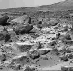
Figure 1: This picture is a grayscale photograph from the Mars Pathfinder mission (http://nssdc.gsfc.nasa.gov/planetary/mesur.html) taken on 4 July, 1997.

Figure 2: This picture is a reconstruction of the photograph in Figure (1) using the first 36 eigenvectors.

Figure 3: This picture is a reconstruction of the photograph in Figure (1) using the first 25 eigenvectors.

We now turn to LSA. Table (1) contains the data used by Landauer et al. (1998) to illustrate LSA. Landauer et al. (1998) constructed an example in which there are two distinct concepts, human-computer interaction (documents c1-c5) and graph theory (documents m1-m4), which share only a single common word “survey”. Frequently occurring words like “and”, “of” and “the” are routinely omitted because they tend to obfuscate an LSA. Landauer et al. (1998) chose words which appear in at least two titles of their small corpus for inclusion in the LSA. As can be seen from Table (1) the word-document matrix is quite sparse.

In Figures (4) through (6) we have the LSA equivalent of the original Mars photograph and its reconstructions described above applied to the word-document matrix in Table (1). Figure (4) is a heatmap of the original matrix and to the human eye the map appears quite sharp. There are only three colours; black, orange and white, corresponding to whether the word occurred zero, once or twice, in a title. Figure (5) is analogous to Figure (2). It is “blurry” to the human eye. In particular, the large black blocks in the upper right and lower left of Figure (4) have become filled with several shades of the brown-orange colour. Figure (6) is analogous to Figure (3) and is blurrier again.

We are now in a position to explain how LSA works. What we would like LSA to do, is to blur the distinction between these words in such a way that if we searched on a word from the human-computer interaction group, it would find all of the documents from that group and none from the graph theory group and vice versa. In rather more technical language we want the SVD and reconstruction of an approximation of the word-document matrix using a smaller number of eigenvectors than the full word-document matrix to extract two non-overlapping groups of words which we can identify as semantic categories. This argument regarding blurring is essentially that put forward by Landuaer (2011) where the blurriness is compared to that which occurs in human vision when squinting.

The reconstructions of the Mars photograph do exactly the same thing, mathematically, as LSA. In the Mars photograph the SVD does not separate the photograph into eigenvectors representing important identifiable features such as sky, rock, pebble, and sand which are then reassembled, feature by feature, in the approximate reconstruction. Rather the eigenvectors are ordered, from largest to smallest, by the amount of variation each accounts for. Discarding the eignevectors corresponding to the smallest eigenvalues removes those eigenvectors which account for the smallest amount of variation in the original. To the human eye this removal of small variation is seen as the loss of fine detail. Consequently the SVD and approximate reconstruction blurs the distinction between sky, rock, pebble, and sand, the extent of the blurring depends on how many eigenvalue-eigenvector pairs are are discarded.

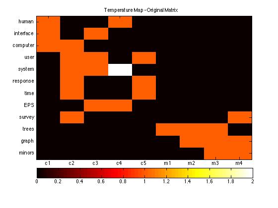
Figure 4: A heatmap of the full word-document matrix in Table (1).

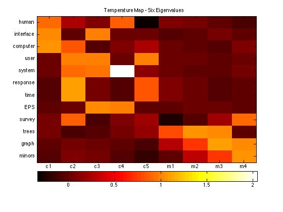
Figure 5: A heatmap of an approximation to the word-document matrix in Table (1) using the six largest eigenvectors.

Figure 6: A heatmap of an approximation to the word-document matrix in Table (1) using the two largest eigenvectors.

Word		“Human”			“Graph”
Rank	Original	6 Eigen	2 Eigen	Original	6 Eigen	2 Eigen
1	c4	c1	c4	m2	m3	m3
2	c1	c4	c2	m3	m4	m4
3	–	c2	c3	m4	m2	m2
4	–	c3	c5	–	m1	c2
5	–	m1	c1	–	c2	m1
6	–	m2	–	–	c3	c5
7	–	–	–	–	–	–
8	–	–	–	–	–	–
9	–	–	–	–	–	–

Table 2: The relevant documents found by a search using “human” and“graph” as the keywords ordered by relevance. The column “Original” uses the orignal full word-document matrix. Column “6 Eigen” uses the six largest eigenvalues and their eigenvectors. Column “2 Eigen” uses the two largest eigenvalues and their eigenvectors.

One of the key steps in LSA is trying to optimize the amount of blurring of the distinction between the words that is undertaken by altering the number of eigenvectors retained in the approximation, see Landauer et al. (1998) Figure (5). In the Landauer et al. (1998) example, the goal of an LSA would be to remove sufficient fine detail from the word-document matrix that the words in the two distinct document groups become relatively indistinguishable, yet retain enough detail that the two groups do not become merged.

Table (2) shows the sets of relevant documents returned by two different keyword searches, one word from each document group, and for each of the three word-document matrices discussed here. From the heatmap of the original matrix (see Figure 4) we can see that it is only possible to find a relevant document if it has a colour other than black. That is, the word must occur in the document or it will not be found. This is exactly what is reported in the two columns labelled “Original” in Table (2).

In Figure (5), the six eigenvalue approximation, document c5 can be seen to have a very low value for “human”, clearly lower than any of the four document in the graph theory document set. In Table (2) the search returned six relevant documents, correctly retrieving c1-c4, but erroneously ranking m1 and m2 as more relevant than the omitted c5. In Figure (6), the two eigenvalue approximation, the extra blurring has made documents c1-c5 more similar to each other when searching on the keyword “human”, but also is now quite distinct from the m1-m4 group. In Table (2) we can see the keyword search has correctly reported c1-c5 as relevant while it excluded all of the graph theory documents. In terms of optimizing the amount of blur in the word-document matrix for the human-computer interaction group the two eigenvalue approximation has done a better job than the six eigenvalue approximation.

The situation is reversed if we search on the word “graph” (second line from the bottom in the heatmaps). In the six eigenvalue approximation it is clear there is very little “heat” associated with the word “graph” in documents c1-c5. The results of the search in Table (2) show that documents m1-m4 are the most relevant but has also included documents c2 and c3. However, in the two eigenvalue approximation document c2, though not relevant, is ranked higher than m1. This time, in terms of optimizing the amount of blur in the word-document matrix for the graph theory group, the six eigenvalue approximation has done a better job than the two eigenvalue approximation.

The type of blurring just discussed is like that seen in Figures (2) and (3) in which the large scale features of the landscape are still visible, fine detail is lost, but there is new “fine detail” in the approximation which was not present in the original, see, for example, the mottled appearance of the sky.

In practice, optimizing the amount of blur is non-trivial and, as indiciated by the simple example, there are trade-offs to be made. This particular example suffers from having only a small number of words and documents, as their numbers increase so does the ability to find an optimum amount of blur in the approximate word-document matrix.

3 Conclusions

The argument put forward in this note, namely that LSA extracts what appears to humans to be semantic meaning is a consequence of the blurring of the distinction between words within a corpus. This idea has been advanced before by one of the originators of LSA. But through the use of simple visualization tools and an analogy to photographic compression, we have made this mechanism much easier to understand for those without the necessary mathematical knowledge to follow the arguments in the existing literature.

References

- Berry et al. (1995) Berry, M. W., S. T. Dumais, and G. W. O’Brien (1995). Using Linear Algebra for Intelligent Information Retrieval. SIAM Review 37(4), 573–595.
- Deerwater et al. (1990) Deerwater, S., S. T. Dumais, F. W. Furnas, T. K. Landauer, and R. Harshman (1990). Indexing by Latent Semantic Analysis. Journal of the American Society for Information Science 41(6), 391–407.
- Gentle (2007) Gentle, J. E. (2007). Matrix Alegbra. Springer.
- Landauer et al. (1998) Landauer, T. K., P. W. Foltz, and D. Laham (1998). An introduction to latent semantic analysis. Discourse Processes 25(2-3), 259–284. http://dx.doi.org/10.1080/0168539809545028.
- Landuaer (2011) Landuaer, T. K. (2011). LSA as a Theory of Meaning. In T. K. Landuaer, D. S. McNamara, S. Dennis, and W. Kintsch (Eds.), Handbook of Latent Semantic Analysis, pp. 3–34. Routledge.
- Landuaer et al. (2011) Landuaer, T. K., D. S. McNamara, S. Dennis, and W. Kintsch (Eds.) (2011). Handbook of Latent Semantic Analysis. Routledge.
- Martin and Berry (2011) Martin, D. I. and M. W. Berry (2011). Mathematical Foundations Behind Latent Semantic Analysis. In T. K. Landuaer, D. S. McNamara, S. Dennis, and W. Kintsch (Eds.), Handbook of Latent Semantic Analysis, pp. 35–55. Routledge.
- Meyer (2000) Meyer, C. D. (2000). Matrix Analysis and Applied Linear Algebra. SIAM.
- NASA (1997) NASA (1997, July). Pathfinder image i1246750998r. http://mars.jpl.nasa.gov/MPF/ops/i1246750998img0008140027.jpg. Accessed 31-Jan-2014.
- Tunkelang (2008) Tunkelang, D. (2008, November). Why does latent semantic analysis work? http://thenoisychannel.com/2008/11/01/why-does-latent-semantic-analysis-work/. Accessed 7-Jan-2014.
- Watkins (2002) Watkins, D. S. (2002). Fundamentals of Matrix Computation (Second ed.). Wiley Inter-Science.