Abstract

Despite seasonal cholera outbreaks in Bangladesh, little is known about the relationship between environmental conditions and cholera cases. We seek to develop a predictive model for cholera outbreaks in Bangladesh based on environmental predictors. To do this, we estimate the contribution of environmental variables, such as water depth and water temperature, to cholera outbreaks in the context of a disease transmission model. We implement a method which simultaneously accounts for disease dynamics and environmental variables in a Susceptible-Infected-Recovered-Susceptible (SIRS) model. The entire system is treated as a continuous-time hidden Markov model, where the hidden Markov states are the numbers of people who are susceptible, infected, or recovered at each time point, and the observed states are the numbers of cholera cases reported. We use a Bayesian framework to fit this hidden SIRS model, implementing particle Markov chain Monte Carlo methods to sample from the posterior distribution of the environmental and transmission parameters given the observed data. We test this method using both simulation and data from Mathbaria, Bangladesh. Parameter estimates are used to make short-term predictions that capture the formation and decline of epidemic peaks. We demonstrate that our model can successfully predict an increase in the number of infected individuals in the population weeks before the observed number of cholera cases increases, which could allow for early notification of an epidemic and timely allocation of resources.

Predictive Modeling of Cholera Outbreaks in Bangladesh
Amanda A. Koepke¹, Ira M. Longini, Jr.², M. Elizabeth Halloran^1,3,
Jon Wakefield^3,4, and Vladimir N. Minin^4,5,∗
1Fred Hutchinson Cancer Research Center, Seattle, Washington, U.S.A.
²Department of Biostatistics and Emerging Pathogens Institute, University of Florida, Gainesville, Florida, U.S.A.
³Department of Biostatistics, University of Washington, Seattle, Washington, U.S.A.
⁴Department of Statistics, University of Washington, Seattle, Washington, U.S.A.
⁵Department of Biology, University of Washington, Seattle, Washington, U.S.A.
$*$email: vminin@uw.edu

1 Introduction

In Bangladesh, cholera is an endemic disease that demonstrates seasonal outbreaks (Huq et al., 2005; Koelle and Pascual, 2004; Koelle et al., 2005; Longini et al., 2002). The burden of cholera is high in that country, with an estimated 352,000 cases and 3,500 to 7,000 deaths annually (International Vaccine Institute, 2012). We seek to understand the dynamics of cholera and to develop a model that will be able to predict outbreaks several weeks in advance. If the timing and size of a seasonal epidemic could be predicted reliably, vaccines and other resources could be allocated effectively to curb the impact of the disease.

Specifically, we want to understand how the disease dynamics are related to environmental covariates. It is currently not known what triggers the seasonal cholera outbreaks in Bangladesh, but it has been shown that Vibrio cholerae, the causative bacterial agent of cholera, can be detected in the environment year round (Huq et al., 1990; Colwell and Huq, 1994). Environmental forces are thought to contribute to the spread of cholera, evident from the many cholera disease dynamics models that incorporate the role of the aquatic environment on cholera transmission through an environmental reservoir effect (Codeço, 2001; Tien and Earn, 2010). One hypothesis is that proliferation of V. cholerae in the environment triggers the seasonal epidemic, feedback from infected individuals drives the epidemic, and then cholera outbreaks wane, either due to an exhaustion of the susceptibles or due to the deteriorating ecological conditions for propagation of V. cholerae in the environment. We probe this hypothesis using cholera incidence data and ecological data collected from multiple thanas (administrative subdistricts with a police station) in rural Bangladesh over sixteen years. There have been three phases of data collection so far, each lasting approximately three years and being separated by gaps of a few years; the current collection phase is ongoing. For a subset of these data, Huq et al. (2005) used Poisson regression to study the association between lagged predictors from a particular water body to cholera cases in that thana. This resulted in different lags and different significant covariates across multiple water bodies and thanas. Thus, it was hard to derive a cohesive model for predicting cholera outbreaks from the environmental covariates. Also, there is no easy way to account for disease dynamics in this Poisson regression framework. We want to measure the effect of the environmental covariates while accounting for disease dynamics via mechanistic models of disease transmission. Moreover, we want to see if we can make reliable short-term predictions with our model — a task that was not attempted by Huq et al. (2005).

Mechanistic infectious disease models use scientific understanding of the transmission process to develop dynamical systems that describe the evolution of the process (Bretó et al., 2009). Realistic models of disease transmission incorporate non-linear dynamics (He et al., 2010), which leads to difficulties with statistical inference under these models, specifically in the tractability of the likelihood. Keeling and Ross (2008) demonstrate some of these difficulties; they use an exact stochastic continuous-time, discrete-state model which evolves Markov processes using the deterministic Kolmogorov forward equations to express the probabilities of being in all possible states. However, that method only works for small populations due to computational limitations. To overcome this intractability, Finkenstädt and Grenfell (2000) develop a time-series Susceptible-Infected-Recovered (SIR) model which extends mechanistic models of disease dynamics to larger populations. A similar development is the auto-Poisson model of Held et al. (2005). To facilitate tractability of the likelihood, both of the above approaches make simplifying assumptions that are difficult to test. Moreover, these discrete-time approaches work only for evenly spaced data or require aggregating the data into evenly spaced intervals. Cauchemez and Ferguson (2008) develop a different, continuous-time, approach to analyze epidemiological time-series data, but assume the transmission parameter and number of susceptibles remain relatively constant within an observation period. Our current understanding of cholera disease dynamics leads us to think that this assumption is not appropriate for modeling endemic cholera with seasonal outbreaks.

To implement a mechanistic approach without these approximations, both maximum likelihood and Bayesian methods can be used. Maximum likelihood based statistical inference techniques use Monte Carlo methods to allow maximization of the likelihood without explicitly evaluating it (He et al., 2010; Bretó et al., 2009; Ionides et al., 2006; Bhadra et al., 2011). Ionides et al. (2006) use this methodology to study how large scale climate fluctuations influence cholera transmission in Bangladesh. Bhadra et al. (2011) use this framework to study malaria transmission in India. They are able to incorporate a rainfall covariate into their model and study how climate fluctuations influence disease incidence when one controls for disease dynamics, such as waning immunity. Under a Bayesian approach, particle filter Markov chain Monte Carlo (MCMC) methods have been developed which require only an unbiased estimate of the likelihood (Andrieu et al., 2010). Rasmussen et al. (2011) use this particle MCMC methodology to simultaneously estimate the epidemiological parameters of a SIR model and past disease dynamics from time series data and gene genealogies. Using Google flu trends data (Ginsberg et al., 2008), Dukic et al. (2012) implement a particle filtering algorithm which sequentially estimates the odds of a pandemic. Notably, Dukic et al. (2012) concentrate on predicting influenza activity. Similarly, here we develop a model-based predictive framework for seasonal cholera epidemics in Bangladesh.

In this paper, we use sequential Monte Carlo methods in a Bayesian framework. Specifically, we develop a hidden Susceptible-Infected-Recovered-Susceptible (SIRS) model for cholera transmission in Bangladesh, incorporating environmental covariates. We use a particle MCMC method to sample from the posterior distribution of the environmental and transmission parameters given the observed data, as described by Andrieu et al. (2010). Further, we predict future behavior of the epidemic within our Bayesian framework. Cholera transmission dynamics in our model are described by a continuous-time, rather than a discrete-time, Markov process to easily incorporate data with irregular observation times. Also, the continuous-time framework allows for greater parameter interpretability and comparability to models based on deterministic differential equations. We test our Bayesian inference procedure using simulated cholera data, generated from a model with a time-varying environmental covariate. We then analyze cholera data from Mathbaria, Bangladesh, similar to the data studied by Huq et al. (2005). Parameter estimates indicate that most of the transmission is coming from environmental sources. We test the ability of our model to make short-term predictions during different time intervals in the data observation period and find that the pattern of predictive distribution dynamics matches the pattern of changes in the reported number of cases. Moreover, we find that the predictive distribution of the hidden states, specifically the unobserved number of infected individuals, clearly pinpoints the beginning of an epidemic approximately two to three weeks in advance, making our methodology potentially useful during cholera surveillance in Bangladesh.

2 SIRS model with environmental predictors

We consider a compartmental model of disease transmission (May and Anderson, 1991; Keeling and Rohani, 2008), where the population is divided into three disease states, or compartments: susceptible, infected, and recovered. We model a continuous process observed at discrete time points. The vector $\mbox{\boldmath$X$}_{t}=(S_{t},I_{t},R_{t})$ contains the numbers of susceptible, infected, and recovered individuals at time $t$, and we consider a closed population of size $N$ such that $N=S_{t}+I_{t}+R_{t}$ for all $t$. Individuals move between the compartments with different rates; for cholera transmission we consider the transition rates shown in Figure 1. In this framework, a susceptible individual’s rate of infection is proportional to the number of infected people and the covariates that serve as proxy for the amount of V. cholerae in the environment. Thus, the hazard rate of infection, also called the force of infection, is $\beta I_{t}+\alpha(t)$ for each time $t$, where $\beta$ represents the infectious contact rate between infected individuals and susceptible individuals and $\alpha(t)$ represents the time-varying environmental force of infection. Possible mechanisms for infectious contact include direct person-to-person transmission of cholera and consumption of water that has been contaminated by infected individuals. Infected individuals recover from infection at a rate $\gamma$, where $1/\gamma$ is the average length of the infectious period. Once the infected individual has recovered from infection, they move to the recovered compartment. Recovered individuals develop a temporary immunity to the disease after infection. They move from the recovered compartment to the susceptible compartment with rate $\mu$, where $1/\mu$ is the average length of immunity. Similar to Codeço (2001) and Koelle and Pascual (2004), birth and death are incorporated into the system indirectly through the waning of immunity; thus, instead of representing natural loss of immunity only, $\mu$ also represents the loss of immunity through the death of recovered individuals and birth of new susceptible individuals.

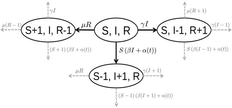
Figure 1: State transitions for Susceptible-Infected-Recovered-Susceptible (SIRS) model for cholera. $S$, $I$, and $R$ denote the numbers of susceptible, infected, and recovered individuals. From the current state $(S,I,R)$, the system can transition to one of three new states. These new states correspond to a susceptible becoming infected, an infected recovering from infection, or a recovered individual losing immunity to infection and becoming susceptible. The parameter $\beta$ is the infectious contact rate, $\alpha(t)$ is the time-varying environmental force of infection, $\gamma$ is the recovery rate, and $\mu$ is the rate at which immunity is lost.

We model $\mbox{\boldmath$X$}_{t}$ as an inhomogeneous Markov process (Taylor and Karlin, 1998) with infinitesimal rates

$$\lambda_{(S,I,R),(S^{\prime},I^{\prime},R^{\prime})}(t)=\left\{\begin{array}[]{rl}\left(\beta I+\alpha(t)\right)S&\mbox{ if $S^{\prime}=S-1$, $I^{\prime}=I+1$, $R^{\prime}=R$},\\ \gamma I&\mbox{ if $S^{\prime}=S$, $I^{\prime}=I-1$, $R^{\prime}=R+1$},\\ \mu R&\mbox{ if $S^{\prime}=S+1$, $I^{\prime}=I$, $R^{\prime}=R-1$},\\ 0&\mbox{ otherwise,}\end{array}\right.$$ (5)

where $\mbox{\boldmath$X$}=(S,I,R)$ is the current state and $\mbox{\boldmath$X$}^{\prime}=(S^{\prime},I^{\prime},R^{\prime})$ is a new state. Because $R_{t}=N-S_{t}-I_{t}$, we keep track of only susceptible and infected individuals, $S_{t}$ and $I_{t}$.

This type of compartmental model is similar to other cholera models in the literature. The time-series SIRS model of Koelle and Pascual (2004) also includes the effects of both intrinsic factors (disease dynamics) and extrinsic factors (environment) on transmission. King et al. (2008) examine both a regular SIRS model and a two-path model to include asymptomatic infections, and use a time-varying transmission term that incorporates transmission via the environmental reservoir and direct person-to-person transmission, but does not allow for feedback from infected individuals into the environmental reservoir. The SIWR model of Tien and Earn (2010) and Eisenberg et al. (2013) allows for infections from both a water compartment (W) and direct transmission and considers the feedback created by infected individuals contaminating the water. To allow for the possibility of asymptomatic individuals, Longini et al. (2007) use a model with a compartment for asymptomatic infections; that model only considers direct transmission. Codeço (2001) uses an SIR model with no direct person-to-person transmission; infected individuals excrete directly into the environment and susceptible individuals are infected from exposure to contaminated water. Our SIRS model is not identical to any of the above models, but it borrows from them two important features: explicit modeling of disease transmission from either direct person-to-person transmission of cholera or consumption of water that has been contaminated by infected individuals and a time-varying environmental force of infection.

3 Hidden SIRS model

While the underlying dynamics of the disease are described by $\mbox{\boldmath$X$}_{t}$, these states are not directly observed. The number $y_{t}$ of infected individuals observed at each time point $t$ is only a random fraction of the number of infected individuals. This fraction depends on both the number of infected individuals that are symptomatic and the fraction of symptomatic infected individuals that seek treatment and get reported (the reporting rate). Thus, $y_{t_{i}}$, the number of observed infections at time $t_{i}$ for observation $i\in\{0,1,...,n\}$, has a binomial distribution with size $I_{t_{i}}$, the number of infected individuals at time $t_{i}$, and success probability $\rho$, the probability of infected individuals seeking treatment, so

$$\mbox{Pr}(y_{t_{i}}|I_{t_{i}},\rho)={I_{t_{i}}\choose y_{t_{i}}}\rho^{y_{t_{i}}}(1-\rho)^{I_{t_{i}}-y_{t_{i}}}.$$ (6)

Given $\mbox{\boldmath$X$}_{t_{i}}$, $y_{t_{i}}$ is independent of the other observations and other hidden states.

We use a Bayesian framework to estimate the parameters of the hidden SIRS model, where the unobserved states $\mbox{\boldmath$X$}_{t}$ are governed by the infinitesimal rates in Equation (5). The parameters that we want to estimate are $\beta$, $\gamma$, $\mu$, $\rho$, and the $k+1$ parameters that will be incorporated into $\alpha(t)$, the time-varying environmental force of infection. We assume $\alpha(t)=\mbox{exp}\left(\alpha_{0}+\alpha_{1}C_{1}(t)+\dots+\alpha_{k}C_{k}(t)\right)$, where $C_{1}(t),\ldots,C_{k}(t)$ denote the $k$ time-varying environmental covariates.

We assume independent Poisson initial distributions for $S_{t_{0}}$ and $I_{t_{0}}$, with means $\phi_{S}$ and $\phi_{I}$. Thus

$$\mbox{Pr}(\mbox{\boldmath$X$}_{t_{0}}|\phi_{S},\phi_{I})=\mbox{Pr}(S_{t_{0}}|\phi_{S})\times\mbox{Pr}(I_{t_{0}}|\phi_{I})=\frac{\phi_{S}^{S_{t_{0}}}\mbox{exp}(-\phi_{S})}{S_{t_{0}}!}\times\frac{\phi_{I}^{I_{t_{0}}}\mbox{exp}(-\phi_{I})}{I_{t_{0}}!}.$$

Parameters that are constrained to be greater than zero, such as $\beta$, $\gamma$, $\mu$, $\phi_{S}$, and $\phi_{I}$, are transformed to the log scale. A logit transformation is used for the probability $\rho$. We assume independent normal prior distributions on all of the transformed parameters, incorporating biological information into the priors where possible.

We are interested in the posterior distribution $\mbox{Pr}(\boldsymbol{\theta}|\mbox{\boldmath$y$})\propto\mbox{Pr}(\mbox{\boldmath$y$}|\boldsymbol{\theta})\mbox{Pr}(\boldsymbol{\theta})$, where $\mbox{\boldmath$y$}=(y_{t_{0}},\ldots,y_{t_{n}})$, $\boldsymbol{\theta}=\left(\mbox{log}(\beta),\mbox{log}(\gamma),\mbox{log}(\mu),\mbox{logit}(\rho),\alpha_{0},\dots,\alpha_{k},\mbox{log}(\phi_{S}),\mbox{log}(\phi_{I})\right)$, and

$$\mbox{Pr}(\mathbf{y}|\boldsymbol{\theta}) = \sum_{\tiny{\mbox{\boldmath$X$}}}\left(\prod_{i=0}^{n}\mbox{Pr}(y_{t_{i}}|I_{t_{i}},\rho)\left[\mbox{Pr}(\mbox{\boldmath$X$}_{t_{0}}|\phi_{S},\phi_{I})\prod_{i=1}^{n}p(\mbox{\boldmath$X$}_{t_{i}}|\mbox{\boldmath$X$}_{t_{i-1}},\boldsymbol{\theta})\right]\right).$$

Here $p(\mbox{\boldmath$X$}_{t_{i}}|\mbox{\boldmath$X$}_{t_{i-1}},\boldsymbol{\theta})$ for $i=1,\ldots,n$ are the transition probabilities of the continuous-time Markov chain (CTMC). However, this likelihood is intractable; there is no practical method to compute the finite time transition probabilities of the SIRS CTMC because the size of the state space of $\mbox{\boldmath$X$}_{t}$ grows on the order of $N^{2}$. For the same reason, summing over $X$ with the forward-backward algorithm (Baum et al., 1970) is not feasible. To use Bayesian inference despite this likelihood intractability, we turn to a particle marginal Metropolis-Hastings (PMMH) algorithm.

4 Particle filter MCMC

4.1 Overview

The PMMH algorithm, introduced by Beaumont (2003) and studied in Andrieu and Roberts (2009) and Andrieu et al. (2010), constructs a Markov chain that targets the joint posterior distribution $\pi(\boldsymbol{\theta},\mbox{\boldmath$X$}|\mathbf{y})$, where $X$ is a set of auxiliary or hidden variables, and requires only an unbiased estimate of the likelihood. To construct this likelihood estimate, we use an SMC algorithm, also known as a bootstrap particle filter (Doucet et al., 2001). The SMC algorithm sequentially estimates the likelihood using weighted particles; it requires the ability to propagate the unobserved data, $\mbox{\boldmath$X$}_{t}$, forward in time and the calculation of the probability of the observed data given the simulated unobserved data. For the hidden SIRS model, $y_{t_{i}}|\mbox{\boldmath$X$}_{t_{i}}=(S_{t_{i}},I_{t_{i}},R_{t_{i}}),\rho\sim\mbox{Binomial}(I_{t_{i}},\rho)$, where $\rho$ depends on the number of symptomatic infected individuals that seek treatment, as described in Section 3. Thus the probability of the observed data given the simulated unobserved data is given by Equation (6). To propagate the hidden variables forward in time, we first simulate initial states $\mbox{\boldmath$X$}_{t_{0}}=\left(S_{t_{0}},I_{t_{0}}\right)$ from Poisson distributions with means $\phi_{S}$ and $\phi_{I}$. We then use properties of CTMCs to simulate the trajectories of the unobserved states.

Thus, the PMMH algorithm has two parts: an SMC algorithm, which is used to estimate the marginal likelihood of the data given a particular set of parameters, $\boldsymbol{\theta}$, and a Metropolis-Hastings step (Metropolis et al., 1953; Hastings, 1970), which uses the estimated likelihood in the acceptance ratio. At each step, a new $\boldsymbol{\theta}^{*}$ is proposed from the proposal distribution $q(\cdot|\boldsymbol{\theta})$. An SMC algorithm is used to generate and weight $K$ particle trajectories corresponding to the hidden state processes using the proposed parameter set $\boldsymbol{\theta}^{*}$. A proposed $\mbox{\boldmath$X$}^{*}_{\mbox{\boldmath$t$}_{0:n}}=\left(\mbox{\boldmath$X$}^{*}_{t_{0}},\ldots,\mbox{\boldmath$X$}^{*}_{t_{n}}\right)$ trajectory is sampled from the $K$ particle trajectories based on the final particle weights of the SMC algorithm. The marginal likelihood is estimated by summing the weights of the SMC algorithm, and the proposed $\boldsymbol{\theta}^{*}$ and $\mbox{\boldmath$X$}^{*}_{\mbox{\boldmath$t$}_{0:n}}$ are accepted with probability equal to the familiar Metropolis-Hastings acceptance ratio.

To propagate the unobserved $\mbox{\boldmath$X$}_{t}=(S_{t},I_{t},R_{t})$ forward in time, we simulate from a cholera transmission model with a time-varying environmental force of infection. CTMCs which incorporate time-varying transition rates are inhomogeneous. The details of the discretely-observed inhomogeneous CTMC simulations are now described.

4.2 Simulating inhomogeneous SIRS using tau-leaping

Gillespie developed two methods for exact stochastic simulation of trajectories with constant rates: the direct method (Gillespie, 1977) and the first reaction method (Gillespie, 1976). Details of these methods are given in Appendix A. The exact algorithms work for small populations, but for large state spaces these methods require a prohibitively long computing time. This is a common problem in the chemical kinetics literature, where an approximate method called the tau-leaping algorithm originated (Gillespie, 2001; Cao et al., 2005). This method simulates CTMCs by jumping over a small amount of time $\tau$ and approximating the number of events that happen in this time using a series of Poisson distributions. As $\tau$ approaches zero, this approximation theoretically approaches the exact algorithm. The value of $\tau$ must be chosen such that the rates remain roughly constant over the period of time; this is referred to as the “leap condition”.

Specifically, for our simulation, using the methods outlined in Cao et al. (2005), we define the rate functions $h_{1}(\mbox{\boldmath$X$}_{t})=\left(\beta I_{t}+\alpha(t)\right)S_{t}$, $h_{2}(\mbox{\boldmath$X$}_{t})=\gamma I_{t}$, and $h_{3}(\mbox{\boldmath$X$}_{t})=\mu R_{t}$, corresponding to the infinitesimal rates of the CTMC. Then $k_{1}\sim\mbox{Poisson}(h_{1}(\mbox{\boldmath$X$}_{t})\tau)$ represents the number of infections in time $[t,t+\tau)$, $k_{2}\sim\mbox{Poisson}(h_{2}(\mbox{\boldmath$X$}_{t})\tau)$ represents the number of recoveries in time $[t,t+\tau)$, and $k_{3}\sim\mbox{Poisson}(h_{3}(\mbox{\boldmath$X$}_{t})\tau)$ represents the number of people that become susceptible to infection in time $[t,t+\tau)$. We make the assumption that the time-varying force of infection, $\alpha(t)$, remains constant each day. We define daily time intervals $A_{i}:=[i,i+1)$ for $i\in\{t_{0},t_{0}+1,\ldots,t_{n}-1\}$, and $\alpha(t)=\alpha_{A_{i}}$ for $t\in A_{i}$. Using $\tau=1$ day, our rates now remain constant within each tau jump. To see if this value for $\tau$ is reasonable, we perform a simulation study; see Appendix A for details.

4.3 Metropolis-Hastings proposal for model parameters

Our implementation of the PMMH algorithm starts with a preliminary run, which consists of a burn-in run plus a secondary run, both using independent normal random walk proposal distributions for the parameters. From the secondary run, we calculate the approximate posterior covariance of the parameters and use it to construct the covariance of the multivariate normal random walk proposal distribution in the final run of the PMMH algorithm. In all runs, parameters are proposed and updated jointly.

4.4 Prediction

One of the main goals of this analysis is to be able to predict cholera outbreaks in advance using environmental predictors. To assess the predictive ability of our model, we estimate the parameters of the model using a training set of data and then predict future behavior of the epidemic process. We examine the posterior predictive distributions of cholera counts by simulating data forward in time under the time-varying SIRS model using the accepted parameter values explored by the particle MCMC algorithm and the accepted values of the hidden states $S_{T}$ and $I_{T}$ at the final observation time, $t=T$, of the training data. These hidden states are sampled in the PMMH algorithm by sampling the last set of particles using the last set of weights (Andrieu et al., 2010). Under each set of parameters, we generate possible future hidden states and observed data, and we compare the posterior predictive distribution of observed cholera cases to the test data. In the analyses below, the PMMH output is always thinned to 500 iterations for prediction purposes by saving only every $k$th iteration, where $k$ depends on the total number of iterations.

5 Simulation results

To test the PMMH algorithm on simulated infectious disease data, we generate data from a hidden SIRS model with a time-varying environmental force of infection. We then use our Bayesian framework to estimate the parameters of the simulated model and compare the posterior distributions of the parameters with the true values. To simulate endemic cholera where many people have been previously infected, we start with a population size of $N=10000$ and assume independent Poisson initial distributions for $S_{t_{0}}$ and $I_{t_{0}}$, with means $\phi_{S}=2100$ and $\phi_{I}=15$. The other parameters are set at $\beta=1.25\times 10^{-5}$, $\gamma=0.1$, and $\mu=0.0009$. All rates are measured in the number of events per day. The average length of the infectious period, $1/\gamma$, is set to be 10 days, and the average length of immunity, $1/\mu$, is set to be about 3 years. Parameter values are chosen such that the simulated data are similar to the data collected from Mathbaria, Bangladesh. We use the daily time intervals $A_{i}:=[i,i+1)$ for $i\in\{t_{0},t_{0}+1,\ldots,t_{n}-1\}$, as in Section 4.2, and define $\alpha(t)=\alpha_{A_{i}}$ for $t\in A_{i}$ where $\alpha_{A_{i}}=\mbox{exp}\left[\alpha_{0}+\alpha_{1}\mbox{sin}\left(2\pi i/365\right)\right].$ The intercept $\alpha_{0}$ and the amplitude $\alpha_{1}$ are parameters to be estimated. The frequency of the sine function is set to mimic the annual peak seen in the environmental data collected from Bangladesh. For the simulations we set $\alpha_{0}=-7$ and $\alpha_{1}=3.5$. Using the modified Gillespie algorithm described in Appendix A, we simulate the $(S_{t},I_{t})$ chain given in the left plot of Figure 2. The observed number of infections $y_{t}\sim\mbox{Binomial}(I_{t},\rho)$, where $\rho=0.015$ and is treated as an unknown parameter.

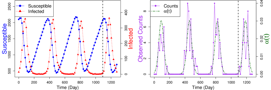
Figure 2: Plots of simulated hidden states (counts of susceptible, $S_{t}$, and infected, $I_{t}$, individuals) and the observed data (number of observed infections $=y_{t}\sim\mbox{Binomial}(I_{t},\rho)$ ) plotted over time, $t$. Simulation with seasonally varying $\alpha(t)$ generates data with seasonal epidemic peaks. The dashed vertical black line represents the first cut off between the training sets and the test data. Data before the line are used to estimate parameters, and we use those estimates to predict the data after the line. Other data cut offs are shown in Figure 3

We simulate three years of training data because this is approximately how long the data collection phases last in our data from Bangladesh (Huq et al., 2005). Therefore we do not attempt to estimate the loss of immunity rate $\mu$ since it is on the scale of three years. Also, there is not enough information in the data to estimate the means of the Poisson initial distributions, $\phi_{S}$ and $\phi_{I}$, since estimation of these parameters is only informed by the very beginning of the observed data. We set these parameters to different values and compare parameter estimation and prediction between models with parameter assumptions which differ from the truth. We also assume that we know the population size, $N=10000$.

We assume normal prior distributions on all of the parameters, with means and standard deviations chosen such that the mass of each prior distribution is not centered at true value of the parameter in this simulation setting. We use relatively uninformative, diffuse priors for $\mbox{log}(\beta)$, $\alpha_{0}$, and $\alpha_{1}$, centered at $\mbox{log}(1.25\times 10^{-4})$, $-8$, and 0, respectively, and with standard deviations of 5. The prior distribution for $\mbox{logit}(\rho)$ is centered at $\mbox{logit}(0.03)$ and has a standard deviation of 2. For $\mbox{log}(\gamma)$, the prior is centered at $\mbox{log}(0.1)$ with a relatively small standard deviation of $0.09$, since this value is well studied for cholera. Thus, a priori $1/\gamma$ falls between 8.4 to 11.9 days with probability 0.95.

Using these data, the PMMH algorithm starts with a burn-in run of 10000 iterations, a secondary run of 10000 iterations, and a final run of 50000 iterations. To thin the chains, we save only every 10th iteration. We use $K=100$ particles in the SMC algorithm. We compare results from models with different assumptions on the values of $\phi_{S}$ and $\phi_{I}$: assumed $\phi_{S}/N$ and $\phi_{I}/N$ are above the true values (0.31 and 0.003), at the true values (0.21 and 0.0015), below the true values (0.11 and 0.00075), or further below the true values (0.055 and 0.000375). Marginal posterior distributions for the parameters of the SIRS model from the final runs of these PMMH algorithms are in Appendix B. The posterior distributions are similar, regardless of assumed values for $\phi_{S}$ and $\phi_{I}$. Trace plots, auto-correlation plots, bivariate scatterplots, and effective sample sizes for the posterior samples under the situation in which the true values of $\phi_{S}$ and $\phi_{I}$ were assumed are also given in Appendix B. We report $\beta\times N$ and $\rho\times N$, since in sensitivity analyses we found these to be robust to assumptions about the total population size $N$. From the posterior distributions, it is clear that the algorithm is providing good estimates of the true parameter values, though estimates of the parameter $\rho\times N$ are slightly different than the truth, especially when $\phi_{S}$ and $\phi_{I}$ are not set at the true values.

5.1 Prediction results

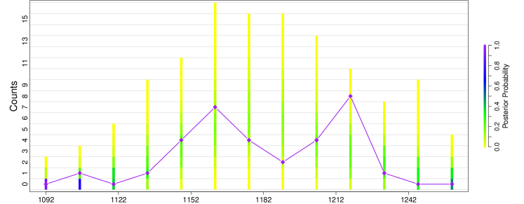
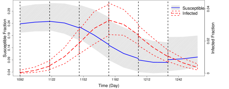
Figure 3: Summary of prediction results for simulated data. We run PMMH algorithms on training sets of the data, which are cut off at each of the dashed black lines in the bottom plot. Future cases are then predicted until the next cut off. The top plot compares the posterior probability of the predicted counts to the test data (diamonds connected by straight purple lines). The coloring of the bars is determined by the frequency of each set of counts in the predicted data for each time point. The bottom plot shows how the trajectory of the predicted hidden states changes over the course of the epidemic. The gray area and the solid line denote the 95% quantiles and median, respectively, of the predictive distribution for the fraction of susceptibles. The short dashed lines and the long dashed line denote the 95% quantiles and median, respectively, of the predictive distribution for the fraction of infected individuals.

To test the predictive ability of the model, we use multiple cut off times to separate our simulated data into staggered training sets and test sets. The simulated observed data are shown in the right plot of Figure 2. For each cut off time, parameters were drawn from the posterior distribution based on the training data. These parameter values were then used to simulate possible realizations of reported infections after the training data until the next cut off, 28 days later. The distributions of these predicted reported cases are shown in the top plot of Figure 3. The test data are denoted by the purple diamonds, connected by straight lines to help visualize ups and downs in the case counts. Case counts are observed once every 14 days. On each observation day, the colored bar represents the distribution of predicted counts for that day. As desired, the posterior predictive distribution shifts its mass as time progresses to follow the case counts in the test data. The plot of the predicted hidden states in the bottom row of Figure 3 also shows that our model is capturing the formation and decline of the epidemic peak well, as seen in the trajectory of the predicted fraction of infected individuals. This plot illustrates the interplay of the hidden states of the underlying compartmental model. During an epidemic, the fraction of susceptibles decreases while the fraction of infected individuals quickly increases. Afterwards, the fraction of infected individuals drops and the pool of susceptibles slowly begins to increase as both immunity is lost and more susceptible individuals are born.

These predictions were made under the assumption that $\phi_{S}$ and $\phi_{I}$ are set to the true values. To test sensitivity to these assumptions, we compare predictions made from models that assume other values; these are shown in Appendix D. Predicted distributions are similar for all values of $\phi_{S}$ and $\phi_{I}$.

6 Using cholera incidence data and covariates from Mathbaria, Bangladesh

Huq et al. (2005) found that water temperature (WT) and water depth (WD) in some water bodies had a significant lagged relationship with cholera incidence. Therefore, we use these covariates and cholera incidence data from Mathbaria, Bangladesh collected between April 2004 to September 2007 and again from October 2010 to July 2013. During these time periods, cholera incidence data were collected over a period of three days approximately every two weeks. Environmental data were also collected approximately every two weeks from six water bodies. To get a smooth summary of the covariates using data from all water bodies, we fit a cubic spline to the covariate values. We then slightly modify our environmental force of infection to allow for a lagged covariate effect. Let $\kappa$ denote the length of the lag. We consider the daily time intervals $A_{i}:=[i,i+1)$ for $i\in\{t_{0},t_{0}+1,\ldots,t_{n}-1\}$ and define the environmental force of infection $\alpha(t)=\alpha_{A_{i}}$ for $t\in A_{i}$ and $t\geq\kappa$ where $\alpha_{A_{i}}=\mbox{exp}\left[\alpha_{0}+\alpha_{1}C_{WD}(i-\kappa)+\alpha_{2}C_{WT}(i-\kappa)\right]$. Here the covariates are the smoothed standardized daily values $C_{WT}(i)=(WT(i)-\overline{WT})/s_{WT}$ and $C_{WD}(i)=(WD(i)-\overline{WD})/s_{WD}$, where $\overline{X}$ is the mean of the measurements for all $i$ and $s_{X}$ is the sample standard deviation. We consider and compare results from models assuming three different lags: $\kappa=14$, $\kappa=18$, and $\kappa=21$. Predictions from all three models are similar, so we report only results from the model assuming $\kappa=21$, in order to receive the earliest warning of upcoming epidemics; see Appendix C for details and prediction comparisons. The smoothed, standardized, 21 day lagged covariates and cholera incidence data are shown in Figure 4.

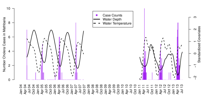
Figure 4: Barplot of cholera case counts in Mathbaria, Bangladesh and the standardized covariate measurements over time. The covariates are shown with a lag of three weeks. No data were collected from October 2007 through November 2010. The ranges of the unstandardized smoothed covariates are 1.4 to 2.8 meters for water depth and 21.6 to 33.1^∘C for water temperature.

Since there are only about six years of data, estimating the loss of immunity rate $\mu$ is infeasible. Thus, we set $\mu=0.0009$ so that $1/\mu$ is 3 years (Sack et al., 2004). Also, the population size $N$, which quantifies the size catchment area for the medical center, is assumed to be 10000 for computational convenience. We do not know the true value of $N$, but 10000 is a reasonable estimate and is small enough that simulations run quickly. We studied sensitivity to these assumptions by setting both $\mu$ and $N$ to different values, obtaining similar results. We also again set $\phi_{S}$ and $\phi_{I}$ to various values and the results were insensitive. See Appendix D for details.

In these analyses, we use relatively uninformative, diffuse normal prior distributions on the time-varying environmental covariates $\alpha_{1}$ and $\alpha_{2}$, centered at 0 and with standard deviations of 5. The diffuse normal prior distributions on the transformed parameter values $\mbox{log}(\beta)$ and $\alpha_{0}$ are centered at $\mbox{log}(1.25\times 10^{-7})$ and $-8$, respectively, with standard deviations of 5. We know that the average infectious period for cholera, $1/\gamma$, should be between 8 and 12 days. Thus, the transformed parameter $\mbox{log}(\gamma)$ is given a normal prior distribution with mean $\mbox{log}(0.1)$ and standard deviation $0.09$ to give 0.95 prior probability of $1/\gamma$ falling within the interval $(8,12)$. We also know that $\rho$ should be very close to zero, since only a small proportion of cholera infections are symptomatic and a smaller proportion will be treated at the health complex (Sack et al., 2003). Thus, the transformed parameter $\mbox{logit}(\rho)$ is given a normal prior distribution with mean $\mbox{logit}(0.0008)$ and standard deviation equal to $2$, to give 0.95 prior probability of $\rho$ falling within the interval $(1.6\times 10^{-5},0.04)$.

We run the PMMH algorithm with a burn-in run of 30000 iterations, a secondary run of 20000 iterations, and a final run of 400000 iterations. We again save only every 10th iteration and use $K=100$ particles in the SMC algorithm. Posterior medians and 95% Bayesian credible intervals for the parameters $\beta\times N$, $\gamma$, $\alpha_{0}$, $\alpha_{1}$, $\alpha_{2}$, and $\rho\times N$ generated by the final run of the PMMH algorithm are given in Table 1. We report $\beta\times N$ and $\rho\times N$ since we found these parameter estimates to be robust to changes in the population size $N$ during sensitivity analyses. For more details, see Appendix D. The credible intervals for $\alpha_{1}$ and $\alpha_{2}$ do not include zero, so both water depth and water temperature have a significant relationship with the force of infection. Decreasing water depth increases the force of infection, likely due to the higher concentration and resulting proliferation of V. cholerae in the environment; increasing water temperature increases the force of infection (Huq et al., 2005).

The basic reproductive number, $R_{0}$, is the average number of secondary cases caused by a typical infected individual in a completely susceptible population (Diekmann et al., 1990). We report $(\beta\times N)/\gamma$, the part of the reproductive number that is related to the number of infected individuals in the population under our model assumptions. Our estimate of 4.35 is fairly large; it is very similar to the reproductive number of 5 (sd=3.3) estimated by Longini et al. (2007) using data from Matlab, Bangladesh. However, the 95% credible interval is wide, with the lower end being approximately 1. Moreover, posterior median values for $\alpha(t)$ range from 0.00003 to 0.38, while posterior median values for $\beta I_{t}$ only range from 0 to 0.03, suggesting that the epidemic peaks in our model are driven mostly by the environmental force of infection. See Appendix F for more details. However, the infectious contact rate is not zero and is not negligible compared to the environmental force of infection.

Table 1: Posterior medians and 95% equitailed credible intervals (CIs) for the parameters of the SIRS model estimated using clinical and environmental data sampled from Mathbaria, Bangladesh.

Coefficient	Estimate	95% CIs
$\beta\times N$	0.491	(0.103 ,	0.945)
$\gamma$	0.115	(0.096 ,	0.142)
$(\beta\times N)/\gamma$	4.35	(0.99 ,	7.15)
$\alpha_{0}$	-5.32	(-6.63 ,	-4.51)
$\alpha_{1}$	-1.37	(-1.98 ,	-0.98)
$\alpha_{2}$	2.18	(1.8 ,	2.62)
$\rho\times N$	55.8	(43.4 ,	73.5)

6.1 Prediction Results

For the data collected from Mathbaria, we begin prediction at multiple points around the time of the two epidemic peaks that occur in 2012 and 2013. Figure 4 shows the full cholera data with smoothed and standardized covariates. Figure 5 shows the posterior predictive distribution of observed cholera cases (top row) and hidden states from the time-varying SIRS model (bottom row). Parameters used to simulate the SIRS forward in time have been sampled using the PMMH algorithm applied to the training data, with data being cut off at different points during the 2012 and 2013 epidemic peaks. From each of these cut offs, parameter values are then used to simulate possible realizations of the test data. Predictions are run until the next cut off point, with cut off points chosen based on the length of the lag $\kappa$. Realistically, at time $t$ we have covariate information to use for prediction only until time $t+\kappa$, where $\kappa$ is the covariate lag. Since the smallest lag considered is 14 days, we make only 14 day ahead predictions where possible to mimic a realistic prediction set up. Due to the sparse sampling between epidemic peaks (June 2012 to February 2013), we use longer prediction intervals for these cut-offs than would be possible in real time data analysis in order to evaluate our model predictions.

In the top row of Figure 5, the coloring of the bars again represents the distribution of predicted cases. Between the two peaks of case counts (June 2012 to February 2013), the frequency of predicted zero counts is very high, so we conclude that the model is doing well with respect to predicting the lack of an epidemic. During the epidemics, the distribution of the counts shifts its mass away from zero. The plot in the bottom row of Figure 5 again illustrates the periodic nature and interplay of the hidden states of the underlying compartmental model. When the fraction of infected individuals quickly increases during an epidemic, the fraction of susceptibles decreases. Afterwards, the fraction of infected individuals drops to almost zero and the pool of susceptibles is slowly replenished. When the fraction of infected individuals is low, there is more uncertainty in the prediction for the fraction of susceptibles (September 2012 to March 2013). The fraction of infected individuals increases to a slightly higher epidemic peak 2013 (March 2013 to May 2013) than in 2012 (March 2012 to May 2012), as observed in the test data for those years. The predicted fraction of infected people in the population increases before an increase can be seen in the case counts, which could allow for early warning of an epidemic.

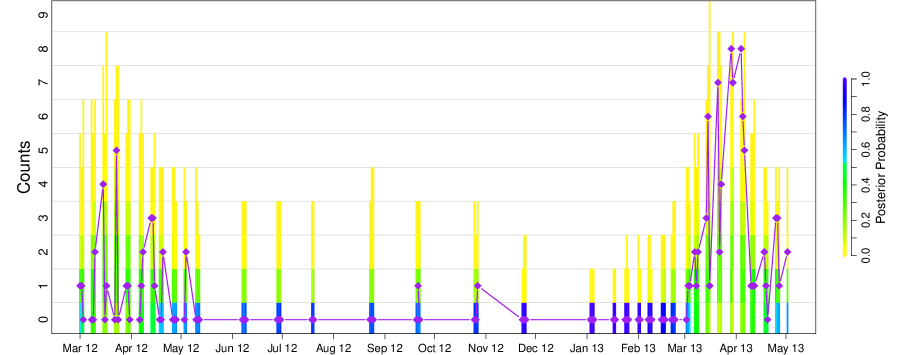
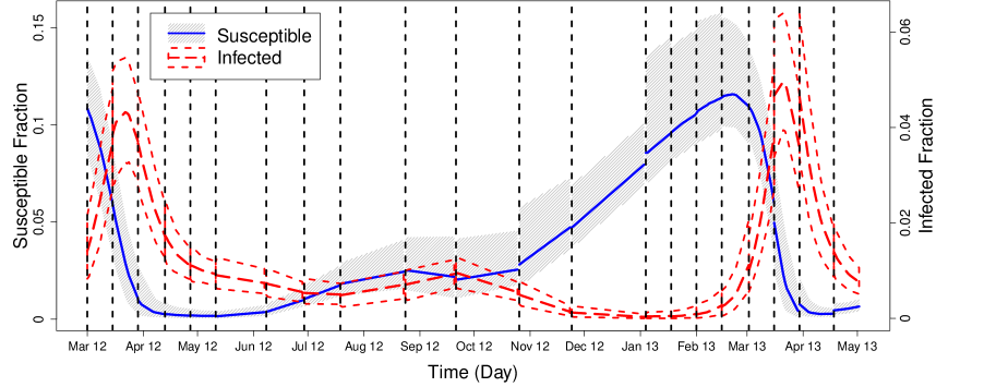
Figure 5: Summary of prediction results for the second to last and last epidemic peaks in the Bangladesh data. We again run PMMH algorithms on training sets of the data, which are cut off at each of the dashed black lines in the bottom plot, and future cases are predicted until the next cut off. The top plot compares the posterior probability of the predicted counts to the test data (purple diamonds and line), and the bottom plot shows how the trajectory of the predicted hidden states changes over the course of the epidemic. See the caption of Figure 3 for more details.

We also use a quasi-Poisson regression model similar to the one used by Huq et al. (2005) to predict the mean number of cholera cases (Appendix E). Although the quasi-Poisson model predicts reasonably well the timing of epidemic peaks, it appears to overestimate the duration of the outbreaks. The predicted means under both the quasi-Poisson and SIRS models most likely underestimate the true mean of the observed counts, with the quasi-Poisson model performing slightly better. However, the SIRS predicted fraction of infected individuals — a hidden variable in the SIRS model — provides a more detailed picture of how cholera affects a population. By providing not only accurate prediction of the time of epidemic peaks, but also the predicted fraction of the population that is infected, the SIRS model predictions could be used for efficient resource allocation to treat infected individuals. See Appendix E for additional details.

7 Discussion

We use a Bayesian framework to fit a nonlinear dynamic model for cholera transmission in Bangladesh which incorporates environmental covariate effects. We demonstrate these techniques on simulated data from a hidden SIRS model with a time-varying environmental force of infection, and the results show that we are recovering well the true parameter values. We also estimate the effect of two environmental covariates on cholera case counts in Mathbaria, Bangladesh while accounting for infectious disease dynamics, and we test the predictive ability of our model. Overall, the prediction results look promising. Based on data collected, the predicted hidden states show a noticeable increase in the fraction of infected individuals weeks before the observed number of cholera cases increases, which could allow for early notification of an epidemic and timely allocation of resources. The predicted hidden states show that the fraction of infected individuals in the population decreases greatly between epidemics, supporting the hypothesis that the environmental force of infection triggers outbreaks. Estimates of $\beta I_{t}$ are low, but not negligible, compared to estimates of $\alpha(t)$, suggesting that most of the transmission is coming from environmental sources.

Computational efficiency is an important factor in determining the usefulness of this approach in the field. We have written an R package which implements the PMMH algorithm for our hidden SIRS model, available at https://github.com/vnminin/bayessir. The computationally expensive portions of the PMMH code are primarily written in C++ to optimize performance, using Rcpp to integrate C++ and R (Eddelbuettel and François, 2011; Eddelbuettel, 2013); however there is still room for improvement. Running $400000$ iterations of the PMMH algorithm on the six years of data from Mathbaria takes 2.5 days on a 4.3 GHz i7 processor. Since we can predict three weeks into the future using a 21 day covariate lag, we do not think timing is a big limitation for using our model predictions in practice.

Plots of residuals over time, shown in Appendix C, show that we are modeling well case counts between the epidemic peaks but not the epidemic peaks themselves, either due to missing the timing of the epidemic peak or the latent states not being modeled accurately. This possible model misspecification might be fixed by including more covariates, using different lags, or modifying the SIRS model. Also, we assume a constant reporting rate, $\rho$, rather than using a time-varying $\rho_{t}$ (Finkenstädt and Grenfell, 2000). With better quality data we might be able to allow for a reporting rate that varies over time; we will try to address these model refinements in future analyses.

In the future, we will extend this analysis to allow for variable selection over a large number of covariates. This will allow us to include many covariates at many different lags and incorporate information from all of the water bodies in a way that does not involve averaging. In the current PMMH framework, choosing an optimal proposal distribution to explore a much larger parameter space would be difficult. We want to include a way of automatically selecting covariates or shrinking irrelevant covariate effects to zero with sparsity inducing priors. The particle Gibbs sampler, introduced by Andrieu et al. (2010), would allow for such extensions. Approximate Bayesian computation is also an option for further model development (McKinley et al., 2009). In addition, the available data consist of observations from multiple thanas during the same time period. Future analyses will look into sharing information across space and time and accounting for correlations between thanas. Another challenging future direction involves exploring models which incorporate a feedback loop from infected individuals back into the environment to capture the effect of infected individuals excreting V. cholerae into the environment. To accomplish this, we could add a water compartment to our SIRS model that quantifies the concentration of V. cholerae in the environment, similar to the model of Tien and Earn (2010). However, adding an additional latent state leads to identifiability problems, even with fully observed data (Eisenberg et al., 2013), so such an extension will require rigorous testing and fine tuning.

Supplementary Materials

Appendix A: Simulation Details

PMMH pseudocode

The following exposition of the algorithm follows closely the pseudocode of Andrieu et al. (2010) and Wilkinson (2011).

Step 1: initialization, for iteration $j=0$,

1. Set $\boldsymbol{\theta}(0)$ arbitrarily

2. Run the following SMC algorithm to get $\hat{p}(\mbox{\boldmath$y$}|\boldsymbol{\theta}(0))$, an estimate of the marginal likelihood, and to produce a sample $\mbox{\boldmath$X$}_{\mbox{\boldmath$t$}_{0:n}}(0)\sim\hat{p}(\cdot|\mbox{\boldmath$y$},\boldsymbol{\theta}(0))$.

   Let the superscript $k\in\{1,\ldots,K\}$ denote the particle index, where $K$ is the total number of particles, and the subscript $t_{i}\in\{t_{0},\ldots,t_{n}\}$ denote the time; thus, $\mbox{\boldmath$X$}_{t_{i}}^{k}$ denotes the $k$th particle at time $t_{i}$, and $\mbox{\boldmath$X$}_{\mbox{\boldmath$t$}_{0:i}}^{k}=\left(\mbox{\boldmath$X$}_{t_{0}}^{k},\ldots,\mbox{\boldmath$X$}_{t_{i}}^{k}\right)$. At time $t_{i}=t_{0}$, sample $\mbox{\boldmath$X$}_{t_{0}}^{k}=(S_{t_{0}}^{k},I_{t_{0}}^{k})$ for $k=1,\ldots,K$ from the initial density of the hidden Markov state process. Specifically, sample $S_{t_{0}}^{k}\sim\mbox{Poisson}(\phi_{S})$ and $I_{t_{0}}^{k}\sim\mbox{Poisson}(\phi_{I})$. Compute the $k$ weights $w(\mbox{\boldmath$X$}_{t_{0}}^{k}):=\mbox{Pr}(y_{t_{0}}|\mbox{\boldmath$X$}_{t_{0}}^{k},\boldsymbol{\theta}(0))={I_{t_{0}}^{k}\choose y_{t_{0}}}\rho(0)^{y_{t_{0}}}(1-\rho(0))^{I_{t_{0}}^{k}-y_{t_{0}}}$, and set $W(\mbox{\boldmath$X$}_{t_{0}}^{k})=w(\mbox{\boldmath$X$}_{t_{0}}^{k})/\sum_{k^{\prime}=1}^{K}w(\mbox{\boldmath$X$}_{t_{0}}^{k^{\prime}})$.

   For $i=1,\ldots,n$, resample $\bar{\mbox{\boldmath$X$}}_{t_{i-1}}^{k}$ from $\mbox{\boldmath$X$}_{t_{i-1}}^{k}$ with weights $W(\mbox{\boldmath$X$}_{t_{i-1}}^{k})$. Sample $K$ particles $\mbox{\boldmath$X$}_{t_{i}}^{k}$ from $p(\cdot|\bar{\mbox{\boldmath$X$}}_{t_{i-1}}^{k})$ (i.e. propagate resampled particles forward one time point). Assign weights $w(\mbox{\boldmath$X$}_{t_{i}}^{k}):=\mbox{Pr}(y_{t_{i}}|\mbox{\boldmath$X$}_{t_{i}}^{k},\boldsymbol{\theta}(0))$ and compute normalized weights $W(\mbox{\boldmath$X$}_{t_{i}}^{k})=w(\mbox{\boldmath$X$}_{t_{i}}^{k})/\sum_{k^{\prime}=1}^{K}w(\mbox{\boldmath$X$}_{t_{i}}^{k^{\prime}})$. Set $\mbox{\boldmath$X$}_{\mbox{\boldmath$t$}_{0:i}}^{k}=(\bar{\mbox{\boldmath$X$}}_{\mbox{\boldmath$t$}_{0:i-1}}^{k},\mbox{\boldmath$X$}_{t_{i}}^{k})$.

   It follows that

   $$\hat{p}(y_{t_{i}}|\mbox{\boldmath$y$}_{\mbox{\boldmath$t$}_{0:i-1}},\boldsymbol{\theta}(0))=\frac{1}{K}\sum_{k=1}^{K}w(\mbox{\boldmath$X$}_{t_{i}}^{k})$$

   is an approximation to the likelihood $p(y_{t_{i}}|\mbox{\boldmath$y$}_{\mbox{\boldmath$t$}_{0:i-1}},\boldsymbol{\theta}(0))$, and therefore an approximation to the total likelihood is

   $$\hat{p}(\mbox{\boldmath$y$}|\boldsymbol{\theta}(0))=\hat{p}(y_{t_{0}}|\boldsymbol{\theta}(0))\prod_{i=1}^{n}\hat{p}(y_{t_{i}}|\mbox{\boldmath$y$}_{\mbox{\boldmath$t$}_{0:i-1}},\boldsymbol{\theta}(0)).$$

   Thus we have a simple, sequential, likelihood-free algorithm which generates an unbiased estimate of the marginal likelihood, $p(\mbox{\boldmath$y$}|\boldsymbol{\theta}(0))$. A $\mbox{\boldmath$X$}_{\mbox{\boldmath$t$}_{0:n}}(0)$ trajectory is sampled from the $K$ trajectories ($\mbox{\boldmath$X$}_{\mbox{\boldmath$t$}_{0:n}}^{k}$, for $k=1,\ldots,K$) based on the final set of particle weights, $W(\mbox{\boldmath$X$}_{t_{n}}^{k})$.

Step 2: for iteration $j\geq 1$,

1. Sample $\boldsymbol{\theta}^{*}\sim q\{\cdot|\boldsymbol{\theta}(j-1)\}$

2. Run an SMC algorithm, as in step 1(b) with $\boldsymbol{\theta}^{*}$ instead of $\boldsymbol{\theta}(0)$, to get $\hat{p}(\mbox{\boldmath$y$}|\boldsymbol{\theta}^{*})$ and $\mbox{\boldmath$X$}^{*}_{\mbox{\boldmath$t$}_{0:n}}\sim\hat{p}(\cdot|\mbox{\boldmath$y$},\boldsymbol{\theta}^{*})$

3. With probability

   $$\mbox{min}\left\{1,\frac{\hat{p}(\mbox{\boldmath$y$}|\boldsymbol{\theta}^{*})}{\hat{p}(\mbox{\boldmath$y$}|\boldsymbol{\theta}(j-1))}\frac{\mbox{Pr}(\boldsymbol{\theta}^{*})}{\mbox{Pr}\{\boldsymbol{\theta}(j-1)\}}\frac{q\{\boldsymbol{\theta}(j-1)|\boldsymbol{\theta}^{*}\}}{q\{\boldsymbol{\theta}^{*}|\boldsymbol{\theta}(j-1)\}}\right\}$$

   set $\boldsymbol{\theta}(j)=\boldsymbol{\theta}^{*}$, $\mbox{\boldmath$X$}_{\mbox{\boldmath$t$}_{0:n}}(j)=\mbox{\boldmath$X$}^{*}_{\mbox{\boldmath$t$}_{0:n}}$, and $\hat{p}(\mbox{\boldmath$y$}|\boldsymbol{\theta}(j))=\hat{p}(\mbox{\boldmath$y$}|\boldsymbol{\theta}^{*})$, otherwise set $\boldsymbol{\theta}(j)=\boldsymbol{\theta}(j-1)$, $\mbox{\boldmath$X$}_{\mbox{\boldmath$t$}_{0:n}}(j)=\mbox{\boldmath$X$}_{\mbox{\boldmath$t$}_{0:n}}(j-1)$, and $\hat{p}(\mbox{\boldmath$y$}|\boldsymbol{\theta}(j))=\hat{p}(\mbox{\boldmath$y$}|\boldsymbol{\theta}(j-1))$.

Simulating homogeneous SIRS

Gillespie’s direct method (Gillespie, 1977) simulates the time to the next event and then determines which event happens at that time. The first reaction method (Gillespie, 1976) calculates the time to the next reaction for each of the possible events, and the minimum time to next reaction determines the next step of the chain.

Using the direct method, we can think of our continuous-time Markov chain (CTMC) as a chemical system with three different reactions. These reactions and their rate functions are given by the infinitesimal rates

$$\lambda_{(S,I,R),(S^{\prime},I^{\prime},R^{\prime})}=\left\{\begin{array}[]{rl}(\beta I+\alpha)S&\mbox{ if $S^{\prime}=S-1$, $I^{\prime}=I+1$, $R^{\prime}=R$},\\ \gamma I&\mbox{ if $S^{\prime}=S$, $I^{\prime}=I-1$, $R^{\prime}=R+1$},\\ \mu R&\mbox{ if $S^{\prime}=S+1$, $I^{\prime}=I$, $R^{\prime}=R-1$},\\ 0&\mbox{ otherwise.}\end{array}\right.$$

Thus the three reactions have the rate functions $h_{1}(\mbox{\boldmath$X$}_{t})=(\beta I_{t}+\alpha)S_{t}$, $h_{2}(\mbox{\boldmath$X$}_{t})=\gamma I_{t}$, and $h_{3}(\mbox{\boldmath$X$}_{t})=\mu R_{t}$, corresponding to the infinitesimal rates of the CTMC. Then the time to the next reaction, $\tau$, has an exponential distribution with rate $\lambda=h_{1}(\mbox{\boldmath$X$}_{t})+h_{2}(\mbox{\boldmath$X$}_{t})+h_{3}(\mbox{\boldmath$X$}_{t})$, and the $k$th reaction occurs with probability $h_{k}(\mbox{\boldmath$X$}_{t})/\lambda$, for $k=\{1,2,3\}$.

The first reaction method instead simulates the time $\tau_{k}$ that the $k$th reaction happens for $k=\{1,2,3\}$, given no other reactions happen in that time. Then the time to the next reaction $\tau=\mbox{min}_{k}(\tau_{k})$, and the reaction with the reaction time equal to $\tau$ is the event that happens.

Both the direct method and the first reaction method work only for homogeneous Markov chains. If we want to assume that the additional force of infection, $\alpha$, varies over time, the associated Markov chain is inhomogeneous and we must account for the fact that the transition rate could change before the next reaction occurs.

Simulating inhomogeneous SIRS

Gibson and Bruck (2000) introduce the next reaction method, an efficient exact algorithm to simulate stochastic chemical systems. They extend this next reaction method to include time-dependent rates and non-Markov processes. Anderson (2007) deviates from these methods a bit, using Poisson processes to represent the reaction times, with time to next reaction given by integrated rate functions. This leads to a more efficient modified next reaction method which they extend to systems with more complicated reaction dynamics.

Using the methods described by Gibson and Bruck (2000) and Anderson (2007), to incorporate a time-varying force of infection into the SIRS model we must integrate over the rate function $h_{1}(\mbox{\boldmath$X$}_{t},s)=\left(\beta I_{t}+\alpha(s)\right)S_{t}$. Thus, to find the time $\tau_{1}$ that the first reaction happens, given no other reactions happen in that time, we generate $u\sim\mbox{Uniform}(0,1)$ and solve

$$\int_{t}^{\tau_{1}}h_{1}(\mbox{\boldmath$X$}_{t},s)ds=\mbox{ln}(1/u)$$

for $\tau_{1}$. Since the other two reactions have no time-varying parameters, we can solve for $\tau_{2}$ and $\tau_{3}$, the reaction times of the second and third reactions, using the methods of the previous section. Then we can continue, using the first reaction method to simulate the process.

We simplify this approach by assuming that the time-varying force of infection, $\alpha(t)$, remains constant each day. We define daily time intervals $A_{i}:=[i,i+1)$ for $i\in\{t_{0},t_{0}+1,\ldots,t_{n}-1\}$, and $\alpha(t)=\alpha_{A_{i}}$ for $t\in A_{i}$. Then we can take advantage of the memoryless property of exponentials and propagate the chain forward in daily increments. Thus, we use the direct method, but when the time to next event exceeds the right end point of the current interval $A_{i}$, we restart CTMC simulation from the beginning of the interval $A_{i+1}$ using $\alpha_{A_{i+1}}$ in the waiting time distribution rate $\lambda(\alpha_{A})=h_{1}(\mbox{\boldmath$X$}_{t},\alpha_{A})+h_{2}(\mbox{\boldmath$X$}_{t})+h_{3}(\mbox{\boldmath$X$}_{t})$, so $\tau\sim\mbox{Exp}(\lambda(\alpha_{A}))$. This modified Gillespie algorithm is depicted and detailed in Figure A-1.

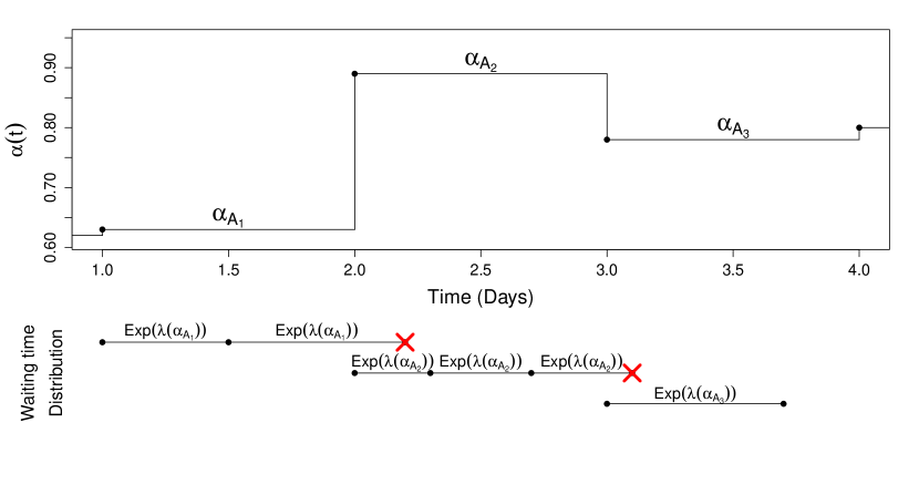
Figure A-1: Depiction of the modified Gillespie algorithm. We assume the environmental force of infection, $\alpha(t)$, is a step function which changes daily. Daily time intervals are denoted by $A_{i}:=[i,i+1)$ for $i\in\{t_{0},t_{0}+1,\ldots,t_{n}-1\}$, so $\alpha(t)=\alpha_{A_{i}}$ for $t\in A_{i}$. Starting at time $t=1$, the waiting time to the next event, $\tau$, has an exponential distribution with rate $\lambda(\alpha_{A_{1}})=h_{1}(\mbox{\boldmath$X$}_{t},\alpha_{A_{1}})+h_{2}(\mbox{\boldmath$X$}_{t})+h_{3}(\mbox{\boldmath$X$}_{t})$. In the depiction, $\tau=0.5$. The simulated waiting time plus the current time, $t^{*}=t+\tau$, remains in the interval $A_{1}$, so we use $t^{*}$ as the next time in our CTMC and propagate $\mbox{\boldmath$X$}_{t}$ forward at that time using Gillespie’s direct method. Since we are still in the interval $A_{1}$, we again simulate the time to the next event as an exponential random variable with rate $\lambda(\alpha_{A_{1}})=h_{1}(\mbox{\boldmath$X$}_{t^{*}},\alpha_{A_{1}})+h_{2}(\mbox{\boldmath$X$}_{t^{*}})+h_{3}(\mbox{\boldmath$X$}_{t^{*}})$. In this iteration, the waiting time plus the current time, $t^{*}+\tau$, exceeds the boundary of the interval $A_{1}$, so we discard this simulated waiting time $\tau$. Using the memoryless property of exponentials, we restart our simulation from the beginning of the interval $A_{2}$ using the new $\alpha(t)$ value, $\alpha_{A_{2}}$. We continue in this manner until we have simulated the Markov process $\mbox{\boldmath$X$}_{t}$ up to time $t_{n}$.

Selecting Tau

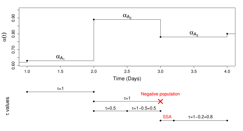
Figure A-2: Depiction of the modified tau-leaping algorithm. We assume the environmental force of infection, $\alpha(t)$, is a step function which changes daily. Daily time intervals are denoted by $A_{i}:=[i,i+1)$ for $i\in\{t_{0},t_{0}+1,\ldots,t_{n}-1\}$, so $\alpha(t)=\alpha_{A_{i}}$ for $t\in A_{i}$. As a default, we use $\tau=1$ day. Starting at time $t=1$, we simulate the changes in compartment populations over the interval $t\in[1,2)$. At time $t=2$, we again use $\tau=1$ day to simulate the changes over the interval $t\in[2,3)$. This value of $\tau$ produces a negative population so we reject that simulation and try again with a smaller $\tau$ (reduced by a factor of $1/2$). The next value of $\tau$ is then calculated based on how long the current daily time-varying force of infection remains constant, so $\tau=0.5$. At time $t=3$, the population of a compartment is lower than some prespecified critical size, so a single step algorithm (SSA), in our case the Gillespie algorithm, is used until the population gets above that critical size. Once the compartment populations are all above the critical size again, at time $t=3.2$, the subsequent value of $\tau$ is again picked based on how long the current daily time-varying force of infection remains constant, so $\tau=0.8$.

Unchecked, tau-leaping can lead to negative population sizes in a compartment if the compartment has a low number of individuals. To avoid this, we use a simplified version of the modified tau-leaping algorithm presented by Cao et al. (2005). If the population of a compartment is lower than some prespecified critical size, a single step algorithm (like the Gillespie algorithm) is used until the population gets above that critical size. If the size of the compartment is not critically low but the current value of $\tau$ still produces a negative population, we reject that simulation and try again with a smaller $\tau$ (reduced by a factor of $1/2$). The subsequent value of $\tau$ is picked based on how long the current daily time-varying force of infection remains constant. We choose a value of $\tau$ that simulates what happens during the remainder of the day, until the value of the transition rate changes. This modified tau-leaping algorithm is depicted and detailed in Figure A-2.

For our simulations, we have chosen $\tau=1$ day; we perform a simulation study to see if this value for $\tau$ is reasonable. Using the posterior estimates of the parameters, we simulate data forward in time 5000 times using both the modified Gillespie algorithm and the modified tau-leaping algorithm. We simulate data over the entire epidemic curve to see how the comparison changes for varying values of $\alpha(t)$. Figure A-3 shows estimates of the median and 95% intervals for the simulated values. The Monte Carlo standard error is very small for all estimates. For the numbers of susceptible individuals, the estimates under Gillespie and tau-leaping are almost identical over the entire epidemic. For the numbers of infected, the values are very close except at the epidemic peaks. However, the differences are very small. We conclude that for our application $\tau=1$ day is a good compromise between computational efficiency and accuracy.

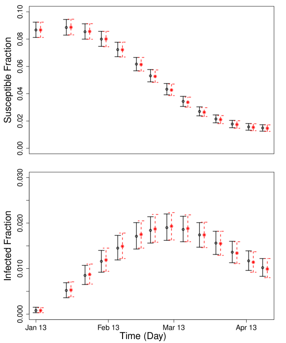
Figure A-3: Plots comparing the median and 95% intervals at different points during an epidemic, simulated using both the modified Gillespie algorithm and the modified tau-leaping algorithm with $\tau=1$ day. The medians and 95% intervals for 5000 simulations using the Gillespie algorithm are given by the open circle and solid error bars. The medians and 95% intervals for 5000 simulations using the modified tau-leaping algorithm are given by the asterisk and dashed error bars.

Binomial tau-leaping

Another solution to the negative population size problem is to use Binomial tau-leaping (Chatterjee et al., 2005; Tian and Burrage, 2004), which further approximates $k_{j}$ as a binomial random variable with mean $h_{j}(\mbox{\boldmath$X$}_{t})\tau$ and upper limit chosen such that $k_{j}$ cannot be large enough to simulate a negative population. We opt instead to use the simplified version of the modified tau-leaping algorithm.

Appendix B: MCMC diagnostics

Using simulated data, we compare results from models with different assumptions on the values of $\phi_{S}$ and $\phi_{I}$; marginal posterior distributions for the parameters of the SIRS model from the final runs of PMMH algorithms are in Figure B-1. The posterior distributions are similar, regardless of assumptions about $\phi_{S}/N$ and $\phi_{I}/N$. Trace plots and autocorrelation plots for the parameters of the SIRS model assuming $\phi_{S}$ and $\phi_{I}$ are set at the true values are in Figure B-2, and Figure B-3 shows bivariate scatterplots of the parameters. Summary plots of the PMMH algorithm output for the parameters of the SIRS model with data from Mathbaria, Bangladesh are given in Figure B-4, and Figure B-5 shows bivariate scatterplots of the parameters. Effective sample sizes range from 593 to 2038 for the parameters of the SIRS model with a time-varying environmental force of infection and from 77 to 1545 for the analysis of the data from Mathbaria. To test convergence, we varied the initial values for the parameters of the PMMH algorithm. Some of the initial values are shown in Table B-1 and the parameter estimates from the chains that started at these initial values are given in the top third of Table B-2. Credible intervals for $\beta\times N$ vary slightly for different initial values; this is likely due to a heavy tail in the posterior distribution that is not yet explored in the run initializing from the second set of starting value and is most often explored in the run initializing at the third set of starting values. If we obtained larger samples from the posterior, the credible intervals would be more similar.

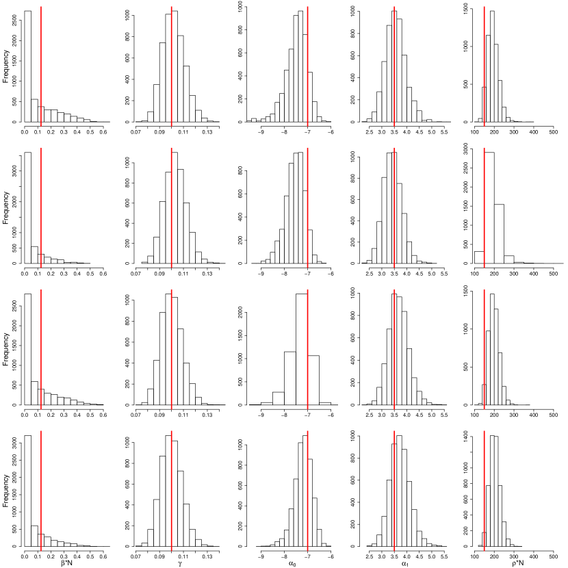
Figure B-1: Posterior distributions for the parameters of the SIRS model, based on simulated data. From top to bottom, the rows have $\phi_{S}/N$ and $\phi_{I}/N$ above the true values (0.31 and 0.003), at the true values (0.21 and 0.0015), below the true values (0.11 and 0.00075), and further below (0.055 and 0.000375). The true values of the parameters are denoted by the red lines.

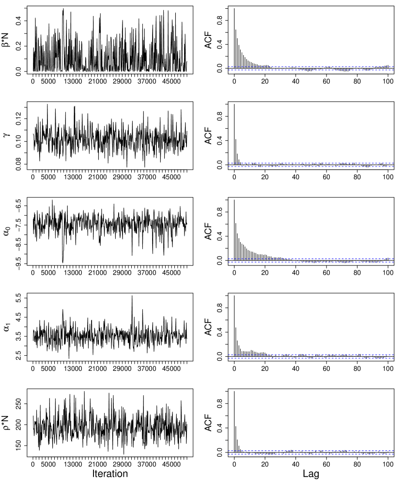
Figure B-2: Summary plots of the PMMH algorithm output (final run of $50000$ iterations) for the parameters of the SIRS model, based on simulated data. ACF plots are thinned to 5000 iterations and trace plots are thinned to display only 500 iterations.

Figure B-3: Bivariate scatterplots of parameters of the SIRS model, based on simulated data. Scatterplots are thinned to display only 200 samples, so only every 250th sample from the posterior distribution is plotted.

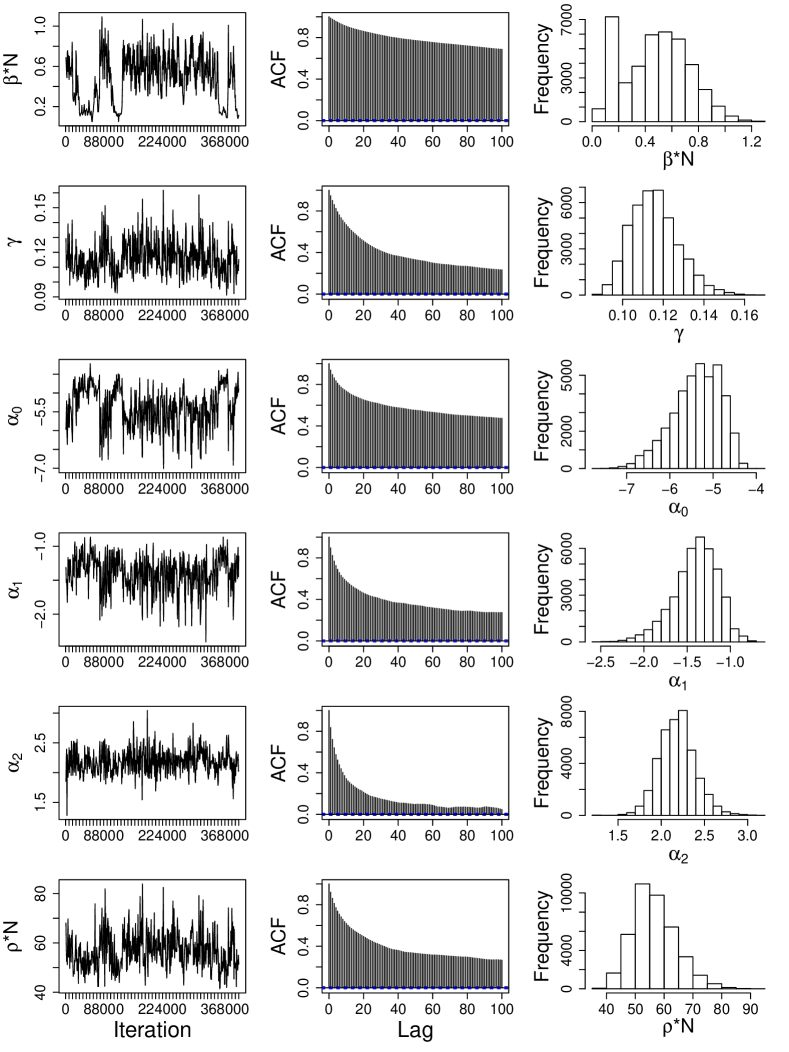
Figure B-4: Summary plots of the PMMH algorithm output (final run of $400000$ iterations) for the parameters of the SIRS model, based on data from Mathbaria, Bangladesh. ACF plots and histograms are thinned to 40000 iterations and trace plots are thinned to display only 500 iterations.

Figure B-5: Bivariate scatterplots of parameters of the SIRS model estimated using data from Mathbaria. Scatterplots are thinned to display only 200 samples, so only every 2000th sample from the posterior distribution is plotted.

Coefficient	Starting value set 1	Starting value set 2	Starting value set 3
$\beta\times N$	0.6	0.8	0.06
$\gamma$	0.11	0.1	0.12
$\alpha_{0}$	$-7.11$	$-8$	$-3$
$\alpha_{1}$	0	0	1
$\alpha_{2}$	0	0	$-1$
$\rho\times N$	60	6	100

Table B-1: Initial values used for separate runs of the PMMH algorithm on the data from Mathbaria. We assume $N=10000$.

	Starting value set 1			Starting value set 2			Starting value set 3
Coefficient	Estimate	95% CIs		Estimate	95% CIs		Estimate	95% CIs
$\beta\times N$	0.49	(0.1 ,	0.95)	0.53	(0.22 ,	0.97)	0.38	(0.02 ,	0.91)
$\gamma$	0.11	(0.1 ,	0.14)	0.12	(0.1 ,	0.14)	0.11	(0.09 ,	0.14)
$(\beta\times N)/\gamma$	4.35	(0.99 ,	7.15)	4.66	(2.05 ,	7.38)	3.48	(0.13 ,	6.97)
$\alpha_{0}$	-5.32	(-6.63 ,	-4.51)	-5.43	(-6.67 ,	-4.71)	-5.12	(-6.46 ,	-4.45)
$\alpha_{1}$	-1.37	(-1.98 ,	-0.98)	-1.41	(-2.02 ,	-1.04)	-1.32	(-1.89 ,	-0.95)
$\alpha_{2}$	2.18	(1.8 ,	2.62)	2.19	(1.8 ,	2.67)	2.17	(1.8 ,	2.57)
$\rho\times N$	55.8	(43.4 ,	73.5)	57	(45.3 ,	73.7)	54.6	(43.9 ,	71.1)
	N=10000, $1/\mu=2$ years			N=5000, $1/\mu=3$ years			N=50000, $1/\mu=3$ years
	$\phi_{S}/N=0.2$, $\phi_{I}/N=0.02$			$\phi_{S}/N=0.2$, $\phi_{I}/N=0.02$			$\phi_{S}/N=0.2$, $\phi_{I}/N=0.02$
Coefficient	Estimate	95% CIs		Estimate	95% CIs		Estimate	95% CIs
$\beta\times N$	0.55	(0.36 ,	0.71)	0.74	(0.35 ,	1.04)	0.8	(0.23 ,	1.04)
$\gamma$	0.12	(0.1 ,	0.14)	0.12	(0.1 ,	0.15)	0.13	(0.11 ,	0.15)
$(\beta\times N)/\gamma$	4.55	(3.21 ,	5.46)	5.94	(3.28 ,	8.07)	6.1	(2.01 ,	7.66)
$\alpha_{0}$	-6.34	(-7.33 ,	-5.29)	-6.12	(-7.8 ,	-4.91)	-6.21	(-7.18 ,	-4.95)
$\alpha_{1}$	-1.83	(-2.38 ,	-1.29)	-1.71	(-2.35 ,	-1.16)	-1.76	(-2.34 ,	-1.19)
$\alpha_{2}$	2.3	(1.8 ,	2.85)	2.14	(1.34 ,	2.74)	2.38	(1.87 ,	2.97)
$\rho\times N$	43.8	(35.6 ,	53.9)	61.5	(47.7 ,	78.7)	65.8	(51.5 ,	81.7)
	N=10000, $1/\mu=3$ years			N=10000, $1/\mu=3$ years			N=10000, $1/\mu=3$ years
	$\phi_{S}/N=0.4$, $\phi_{I}/N=0.04$			$\phi_{S}/N=0.1$, $\phi_{I}/N=0.01$			$\phi_{S}/N=0.4$, $\phi_{I}/N=0.01$
Coefficient	Estimate	95% CIs		Estimate	95% CIs		Estimate	95% CIs
$\beta\times N$	0.99	(0.07 ,	1.25)	0.9	(0.67 ,	1.14)	1.23	(1.03 ,	1.42)
$\gamma$	0.14	(0.1 ,	0.16)	0.12	(0.1 ,	0.14)	0.15	(0.13 ,	0.17)
$(\beta\times N)/\gamma$	7.19	(0.65 ,	9.17)	7.5	(5.98 ,	9.03)	8.27	(6.8 ,	9.88)
$\alpha_{0}$	-6.28	(-7.1 ,	-4.79)	-6.73	(-7.58 ,	-5.68)	-6.59	(-7.22 ,	-5.92)
$\alpha_{1}$	-1.75	(-2.26 ,	-1.13)	-1.96	(-2.45 ,	-1.44)	-1.83	(-2.28 ,	-1.38)
$\alpha_{2}$	2.42	(1.89 ,	2.93)	2.29	(1.79 ,	2.9)	2.71	(2.3 ,	3.15)
$\rho\times N$	68.5	(40.9 ,	83.4)	65.7	(53.2 ,	80.4)	79.2	(65.7 ,	95.4)

Table B-2: Convergence diagnostics and sensitivity analysis: Posterior medians and 95% equitailed credible intervals (CIs) under different initial values and assumptions for the parameters of the SIRS model estimated using clinical and environmental data sampled from Mathbaria, Bangladesh. The PMMH algorithm is run from different initial values using $N=10000$, $1/\mu=3$ years, $\phi_{S}/N=0.2$, and $\phi_{I}/N=0.02$, and also run using different values for the population size, $N$, the loss of immunity rate, $\mu$, and the means of the Poisson initial distributions, $\phi_{S}$ and $\phi_{I}$.

Appendix C: Model fit

To select a lag for the environmental covariates in the Mathbaria analysis, we compare prediction results from models assuming three different lags: $\kappa=14$, $\kappa=18$, and $\kappa=21$. These are shown in Figures C-1 and C-2. The predictive distributions of the hidden states look similar across lags, so we use the 21 day lag model in order to predict an upcoming epidemic furthest in advance. With a three week lag, we would be able to make predictions three weeks in advance.

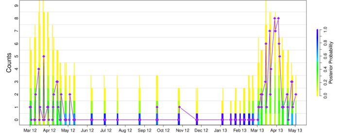
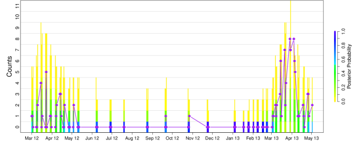
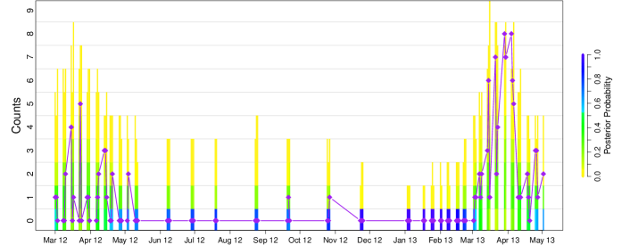
Figure C-1: Distributions of predicted reported cases under models assuming a covariate lag of 14 days (top), 18 days (middle), and 21 days (bottom). The posterior probability of the predicted counts is compared to the test data (diamonds connected by straight line). The coloring of the bars is determined by the frequency of each set of counts in the predicted data for each time point. The distributions are similar, regardless of lag choice.

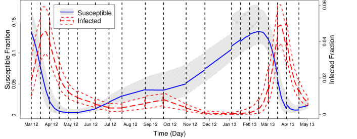
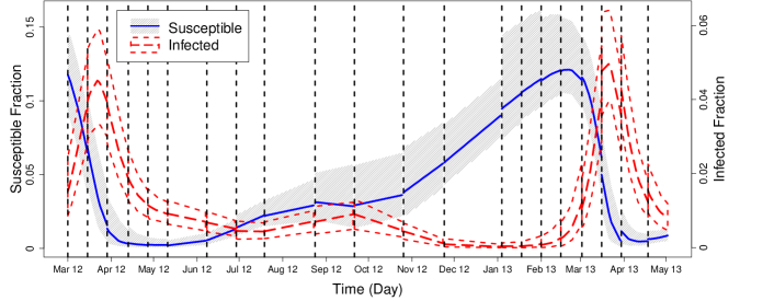
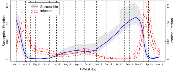
Figure C-2: Predictive distributions of the hidden states, under models assuming a covariate lag of 14 days (top), 18 days (middle), and 21 days (bottom). The gray area and the solid line denote the 95% quantiles and median of the predictive distributions for the fraction of susceptibles. The short dashed lines and the long dashed line denote the 95% quantiles and median of the predictive distributions for the fraction of infected individuals. Differences between the distributions under the different lags are difficult to distinguish.

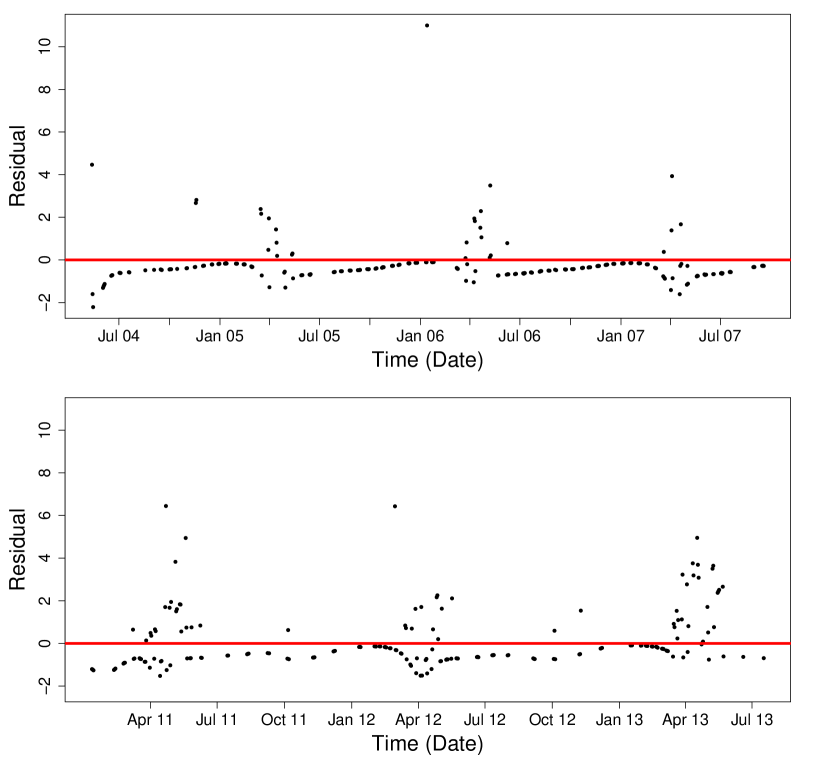
Figure C-3: Plot of standardized residuals versus time. The top figure shows the residuals for the first three years of data collected from Bangladesh, and the bottom figure shows the residuals for the second three years of data collection. The red line is drawn through zero for reference.

Figure C-3 shows plots of standardized residuals versus time for each of the two phases of data collection in Mathbaria, Bangladesh. Standardized residuals are calculated as $\epsilon_{t_{i}}=\left(y_{t_{i}}-\mbox{E}(y_{t_{i}})\right)/\mbox{sd}(y_{t_{i}})$, where $y_{t_{i}}$ is the number of observed infections at time $t_{i}$ for observation $i\in\{0,1,...,n\}$. $\mbox{E}(y_{t_{i}})$ and $\mbox{sd}(y_{t_{i}})$ are approximated via simulation by fixing the model parameters to the posterior medians, running the SIRS model forward 5000 times, and computing the average and sample standard deviation of the 5000 realizations of the case counts at each time point. Residuals are furthest from zero during the epidemic peaks; the inflation of residuals during times of high case counts is probably due to the model being off in terms of the timing of the epidemic peak or the latent states not being predicted correctly.

Appendix D: Sensitivity analysis

In our analysis of the data from Mathbaria, we assumed the size of the population, $N=10000$, the loss of immunity rate, $\mu=0.0009$, and the means of the Poisson initial distributions, $\phi_{S}=.2\times N$ and $\phi_{I}=0.02\times N$, are known. We studied sensitivity to these assumptions by setting all of these parameters to different values, and the results are shown in the bottom two-thirds of Table B-2. We report $\beta\times N$ and $\rho\times N$ since we found these parameter estimates to be robust to changes in the population size $N$. As seen in Table B-2, estimates are similar over different values of $N$, $\mu$, $\phi_{S}$ and $\phi_{I}$.

We also tested the effect of incorrect values for $\phi_{S}$ and $\phi_{I}$ on prediction using simulated data, as seen in Figure D-1. Values for $\phi_{S}/N$ and $\phi_{I}/N$ are set above the true values, (0.31, 0.003), at the truth (0.21, 0.0015), under the true values (0.11, 0.00075), and further under the truth (0.055, 0.000375). Predicted distributions look similar for all values of $\phi_{S}$ and $\phi_{I}$. Uncertainty is greatest when $\phi_{S}$ and $\phi_{I}$ are set at higher values than the truth. For the lowest values of $\phi_{S}$ and $\phi_{I}$, the fraction of susceptible individuals is lower and the fraction of infected is higher than those predicted fractions under other settings. However, important information, like the timing of the epidemic, remains intact.

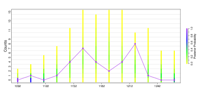
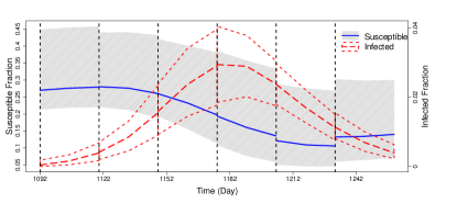
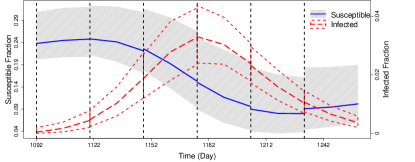
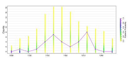
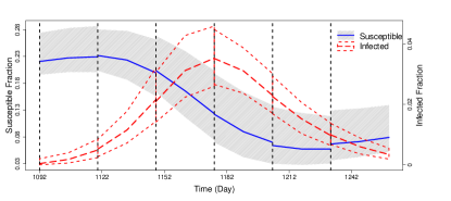
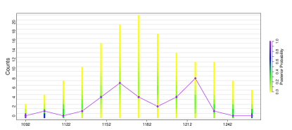
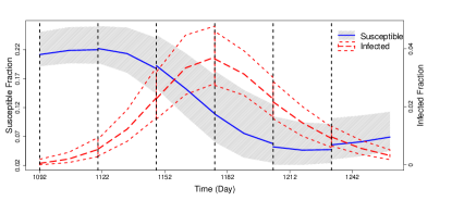
Figure D-1: Summary of prediction results for simulated data; each row shows prediction results under different assumptions about the values of $\phi_{s}/N$ and $\phi_{I}/N$. From top to bottom, values for $\phi_{S}/N$ and $\phi_{I}/N$ are set above the true values, (0.31, 0.003), at the truth (0.21, 0.0015), under the true values (0.11, 0.00075), and further under (0.055, 0.000375). Plots on the left compare the posterior probability of the predicted counts to the test data (diamonds connected by straight line). The coloring of the bars is determined by the frequency of each set of counts in the predicted data for each time point. The plots on the right show how the trajectory of the predicted hidden states change over the course of the epidemic. The gray area and the solid line denote the 95% quantiles and median of the predictive distribution for the fraction of susceptibles. The short dashed lines and the long dashed line denote the 95% quantiles and median of the predictive distribution for the fraction of infected individuals.

Appendix E: Prediction

We compare SIRS predictive distributions to predictions made from a lagged quasi-Poisson regression model, similar to the one used by Huq et al. (2005). For the two predictors, water temperature (WT) and water depth (WD), we have

$$\mbox{ln}\mbox{ E}(Y_{t}|C_{WD}(t-\kappa),C_{WT}(t-\kappa))=\beta_{0}+\beta_{1}C_{WD}(t-\kappa)+\beta_{2}C_{WT}(t-\kappa),$$

where $\kappa=21$ days. The quasi-Poisson model accounts for overdispersion in the data (McCullagh and Nelder, 1989). Figure E-1 shows the predicted means and 95% intervals under the quasi-Poisson model. Test data are again cut off at different points during the 2012 and 2013 epidemic peaks and predictions are run until the next cut off point, with cut off points chosen approximately every two weeks. Predicted mean number of reported cases and 95% intervals from the hidden SIRS model are also shown for comparison. To calculate these, we sample 500 sets of parameter values from the posterior. For each set of parameters, we simulate data forward until the next cut off point 100 times and then calculate the mean of the predicted counts at each observation time. Using these 500 means from the 500 parameter sets, we calculate the overall predicted means and 95% intervals. Both models predict well the timing of epidemic peaks. However, the quasi-Poisson regression framework does not provide any information about the underlying fraction of infected individuals in the population, which may be important for resource allocation.

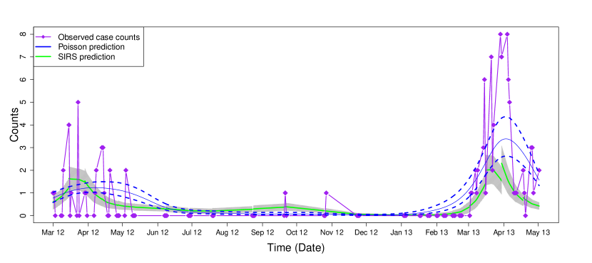
Figure E-1: Comparison of predicted means for number of reported cases. The solid blue lines and the dashed blue lines denote the predicted means and 95% intervals under the quasi-Poisson model. The green line and gray area denote the predicted means and 95% intervals under the SIRS model. Predictions are started and stopped using identical cut-off points for the training and test data to those in Figure 5. Test data are denoted by the purple diamonds connected by straight lines.

Appendix F: Routes of transmission

An important question in cholera modeling is: what is the relative contribution of different routes of transmission at different points of the epidemic? We hypothesized that environmental forces trigger the seasonal cholera epidemics and that infectious contact between susceptible and infected individuals drives the epidemics. To examine this possible dynamic, we compare the forces of infection from the environment, $\alpha(t)$, to that from infected individuals, $\beta\times I_{t}$, over time. Values are computed by sampling 5000 sets of parameter values from the posterior. For each set of parameters, we generate data using our hidden SIRS model. Figure F-1 shows median and 95% quantiles for $\alpha(t)$ vs $\beta\times I_{t}$ plotted over time. The median values of $\alpha(t)$ are almost always higher than values of $\beta\times I_{t}$; the only time it is not (in early 2011) is most likely caused by model misspecification, specifically in setting $\phi_{I}$ to the wrong value for this phase. This model misspecification is similarly reflected in Figure C-3. This supports the hypothesis that the epidemics are driven by the environmental force of infection.

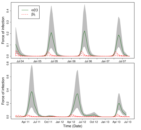
Figure F-1: The relative contribution of different routes of transmission at different points of the epidemic curves. The gray area and the solid line denote the 95% quantiles and median of the force of infection from the environment, $\alpha(t)$. The long dashed lines and the short dashed line denote the 95% quantiles and median of the force of infection from infected individuals, $\beta\times I_{t}$.

References

- Anderson [2007] D. F. Anderson. A modified next reaction method for simulating chemical systems with time dependent propensities and delays. Journal of Chemical Physics, 127(21):214107, 2007.
- Andrieu and Roberts [2009] C. Andrieu and G. O. Roberts. The pseudo-marginal approach for efficient Monte Carlo computations. The Annals of Statistics, 37(2):697–725, 2009.
- Andrieu et al. [2010] C. Andrieu, A. Doucet, and R. Holenstein. Particle Markov chain Monte Carlo methods. Journal of the Royal Statistical Society: Series B (Statistical Methodology), 72(3):269–342, 2010.
- Baum et al. [1970] L. E. Baum, T. Petrie, G. Soules, and N. Weiss. A maximization technique occurring in the statistical analysis of probabilistic functions of Markov chains. The Annals of Mathematical Statistics, 41(1):164–171, 1970.
- Beaumont [2003] M. A. Beaumont. Estimation of population growth or decline in genetically monitored populations. Genetics, 164(3):1139–1160, 2003.
- Bhadra et al. [2011] A. Bhadra, E. L. Ionides, K. Laneri, M. Pascual, M. Bouma, and R. C. Dhiman. Malaria in Northwest India: Data analysis via partially observed stochastic differential equation models driven by Lévy noise. Journal of the American Statistical Association, 106(494):440–451, 2011.
- Bretó et al. [2009] C. Bretó, D. He, E. L. Ionides, and A. A. King. Time series analysis via mechanistic models. Annals of Applied Statistics, 3(1):319–348, 2009.
- Cao et al. [2005] Y. Cao, D. T. Gillespie, and L. R. Petzold. Avoiding negative populations in explicit Poisson tau-leaping. The Journal of Chemical Physics, 123(5):054104, 2005.
- Cauchemez and Ferguson [2008] S. Cauchemez and N. M. Ferguson. Likelihood-based estimation of continuous-time epidemic models from time-series data: application to measles transmission in London. Journal of the Royal Society Interface, 5(25):885–897, 2008.
- Chatterjee et al. [2005] A. Chatterjee, D. G. Vlachos, and M. A. Katsoulakis. Binomial distribution based -leap accelerated stochastic simulation. The Journal of Chemical Physics, 122:024112, 2005.
- Codeço [2001] C. Codeço. Endemic and epidemic dynamics of cholera: the role of the aquatic reservoir. BMC Infectious Diseases, 1(1):1, 2001.
- Colwell and Huq [1994] R. R. Colwell and A. Huq. Environmental reservoir of Vibrio cholerae: The causative agent of cholera. Annals of the New York Academy of Sciences, 740(1):44–54, 1994.
- Diekmann et al. [1990] O. Diekmann, J. A. P. Heesterbeek, and J. A. J. Metz. On the definition and the computation of the basic reproductive ratio R0 in models for infectious diseases in heterogeneous populations. Mathematical Biology, 28:365–382, 1990.
- Doucet et al. [2001] A. Doucet, N. De Freitas, and N. Gordon. Sequential Monte Carlo Methods in Practice. Springer, 2001.
- Dukic et al. [2012] V. Dukic, H. F. Lopes, and N. G. Polson. Tracking epidemics with Google flu trends data and a state-space SEIR model. Journal of the American Statistical Association, 107(500):1410–1426, 2012.
- Eddelbuettel [2013] D. Eddelbuettel. Seamless R and C++ Integration with Rcpp. Springer, New York, 2013.
- Eddelbuettel and François [2011] D. Eddelbuettel and R. François. Rcpp: Seamless R and C++ integration. Journal of Statistical Software, 40(8):1–18, 2011.
- Eisenberg et al. [2013] M. C. Eisenberg, S. L. Robertson, and J. H. Tien. Identifiability and estimation of multiple transmission pathways in cholera and waterborne disease. Journal of Theoretical Biology, 324(0):84–102, 2013.
- Finkenstädt and Grenfell [2000] B. F. Finkenstädt and B. T. Grenfell. Time series modelling of childhood diseases: a dynamical systems approach. Journal of the Royal Statistical Society: Series C (Applied Statistics), 49(2):187–205, 2000.
- Gibson and Bruck [2000] M. A. Gibson and J. Bruck. Efficient exact stochastic simulation of chemical systems with many species and many channels. The Journal of Physical Chemistry A, 104(9):1876–1889, 2000.
- Gillespie [1976] D. T. Gillespie. A general method for numerically simulating the stochastic time evolution of coupled chemical reactions. Journal of Computational Physics, 22(4):403–434, 1976.
- Gillespie [1977] D. T. Gillespie. Exact stochastic simulation of coupled chemical reactions. The Journal of Physical Chemistry, 81(25):2340–2361, 1977.
- Gillespie [2001] D. T. Gillespie. Approximate accelerated stochastic simulation of chemically reacting systems. The Journal of Chemical Physics, 115(4):1716–1733, 2001.
- Ginsberg et al. [2008] J. Ginsberg, M. H. Mohebbi, R. S. Patel, L. Brammer, M. S. Smolinski, and L. Brilliant. Detecting influenza epidemics using search engine query data. Nature, 457(7232):1012–1014, 2008.
- Hastings [1970] W. K. Hastings. Monte Carlo sampling methods using Markov chains and their applications. Biometrika, 57:97–109, 1970.
- He et al. [2010] D. He, E. L. Ionides, and A. A. King. Plug-and-play inference for disease dynamics: measles in large and small populations as a case study. Journal of the Royal Society Interface, 7:271–283, June 2010.
- Held et al. [2005] L. Held, M. Höhle, and M. Hofmann. A statistical framework for the analysis of multivariate infectious disease surveillance counts. Statistical Modelling, 5(3):187–199, 2005.
- Huq et al. [1990] A. Huq, R. R. Colwell, R. Rahman, A. Ali, MA Chowdhury, S. Parveen, D. A. Sack, and E. Russek-Cohen. Detection of Vibrio cholerae O1 in the aquatic environment by fluorescent-monoclonal antibody and culture methods. Applied and Environmental Microbiology, 56(8):2370–2373, 1990.
- Huq et al. [2005] A. Huq, R. B. Sack, A. Nizam, I. M. Longini, G. B. Nair, A. Ali, J. G. Morris Jr, M. N. Khan, A. K. Siddique, M. Yunus, M. J. Albert, D. A. Sack, and R. R. Colwell. Critical factors influencing the occurrence of Vibrio cholerae in the environment of Bangladesh. Applied and Environmental Microbiology, 71(8):4645–4654, 2005.
- International Vaccine Institute [2012] International Vaccine Institute. Country investment case study on cholera vaccination: Bangladesh. International Vaccine Institute, Seoul, 2012.
- Ionides et al. [2006] E. L. Ionides, C. Bretó, and A. A. King. Inference for nonlinear dynamical systems. Proceedings of the National Academy of Sciences, 103(49):18438–18443, 2006.
- Keeling and Rohani [2008] M. J. Keeling and P. Rohani. Modeling Infectious Diseases in Humans and Animals. Princeton University Press, 2008.
- Keeling and Ross [2008] M. J. Keeling and J. V. Ross. On methods for studying stochastic disease dynamics. Journal of The Royal Society Interface, 5(19):171–181, 2008.
- King et al. [2008] A. A. King, E. L. Ionides, M. Pascual, and M. J. Bouma. Inapparent infections and cholera dynamics. Nature, 454(7206):877–880, 2008.
- Koelle and Pascual [2004] K. Koelle and M. Pascual. Disentangling extrinsic from intrinsic factors in disease dynamics: a nonlinear time series approach with an application to cholera. The American Naturalist, 163(6):901–913, 2004.
- Koelle et al. [2005] K. Koelle, X. Rodó, M. Pascual, M. Yunus, and G. Mostafa. Refractory periods and climate forcing in cholera dynamics. Nature, 436(7051):696–700, 2005.
- Longini et al. [2002] I. M. Longini, M. Yunus, K. Zaman, A. K. Siddique, R. B. Sack, and A. Nizam. Epidemic and endemic cholera trends over a 33-year period in Bangladesh. Journal of Infectious Diseases, 186(2):246–251, 2002.
- Longini et al. [2007] I. M. Longini, Jr., A. Nizam, M. Ali, M. Yunus, N. Shenvi, and J. D. Clemens. Controlling endemic cholera with oral vaccines. PLoS medicine, 4(11):e336, 2007.
- May and Anderson [1991] R. May and R. M. Anderson. Infectious Diseases of Humans: Dynamics and Control. Oxford University Press, 1991.
- McCullagh and Nelder [1989] P. McCullagh and J. A. Nelder. Generalized Linear Models. Chapman & Hall/CRC, 1989.
- McKinley et al. [2009] T. McKinley, A. R. Cook, and R. Deardon. Inference in epidemic models without likelihoods. The International Journal of Biostatistics, 5:–, 2009.
- Metropolis et al. [1953] N. Metropolis, A. W. Rosenbluth, M. N. Rosenbluth, A. H. Teller, and E. Teller. Equation of state calculations by fast computing machines. Journal of Chemical Physics, 21(6):1087–1092, 1953.
- Rasmussen et al. [2011] D. A. Rasmussen, O. Ratmann, and K. Koelle. Inference for nonlinear epidemiological models using genealogies and time series. PLoS Computational Biology, 7(8):e1002136, 2011.
- Sack et al. [2004] D. A. Sack, R. B. Sack, G. B. Nair, and A. K. Siddique. Cholera. The Lancet, 363(9404):223–233, 2004.
- Sack et al. [2003] R. B. Sack, A. K. Siddique, I. M. Longini, A. Nizam, M. Yunus, S. Islam, J. G. Morris, A. Ali, A. Huq, G. B. Nair, F. Qadri, Shah, M. Faruque, D. A. Sack, and R. R. Colwell. A 4-year study of the epidemiology of Vibrio cholerae in four rural areas of Bangladesh. Journal of Infectious Diseases, 187(1):96–101, 2003.
- Taylor and Karlin [1998] H. M. Taylor and S. Karlin. An Introduction to Stochastic Modeling. Academic Press, 3rd edition, 1998.
- Tian and Burrage [2004] T. Tian and K. Burrage. Binomial leap methods for simulating stochastic chemical kinetics. The Journal of Chemical Physics, 121:10356–10364, 2004.
- Tien and Earn [2010] J. H. Tien and D. J. D. Earn. Multiple transmission pathways and disease dynamics in a waterborne pathogen model. Bulletin of Mathematical Biology, 72(6):1506–1533, 2010.
- Wilkinson [2011] D. J. Wilkinson. Stochastic Modelling for Systems Biology. CRC press, 2nd edition, 2011.