Influence of Magnetorotational Instability on Neutrino Heating: A New Mechanism for Weakly Magnetized Core-Collapse Supernovae

Abstract

We investigated the impacts of magnetorotational instability (MRI) on the dynamics of weakly magnetized, rapidly rotating core-collapse by conducting high resolution MHD simulations in axisymmetry with simplified neutrino transfer. We found that an initially sub-magnetar class magnetic field is drastically amplified by MRI and substantially affects the dynamics thereafter. Although the magnetic pressure is not strong enough to eject matter, the amplified magnetic field efficiently transfers angular momentum from higher to lower latitudes, which causes the expansion of the heating region at low latitudes due to the extra centrifugal force. This then enhance the efficiency of neutrino heating and eventually leads to neutrino-driven explosion. This is a new scenario of core-collapse supernovae that has never been demonstrated by numerical simulations so far.

1. Introduction

At present neutrino heating is considered to be the most promising candidate for the as-yet-unknown explosion mechanism of core-collapse supernovae (CCSNe). Recent state-of-the-art simulations with detailed neutrino transport have not yet succeeded in reproducing the canonical explosion energy of $10^{51}$ erg, though (e.g., Suwa et al., 2010; Müller et al., 2012; Bruenn et al., 2013). Other effects to enhance or drive explosion may hence be required.

Magnetic field and rotation may bring such effects. Although the magnetic field and rotation of progenitors at the pre-collapse stage are not well-understood, some of recent theoretical and observational studies indicate that their strengths may spread over a wide range.

Optical observations of OB main sequence stars reported recently that some of them possess $\sim 1$ kG surface magnetic fields (e.g., Wade et al., 2012), which correspond to the magnetar-class magnetic flux, $\sim 10^{26}$–$10^{27}$ G cm². A population synthesis calculation assuming the conservation of magnetic flux during the post-main-sequence evolution performed by Ferrario & Wickramasinghe (2006) indicates that $\sim 10$% of OB stars have the magnetar-class magnetic flux, while the majority has $\sim$1–2 orders of magnitude weaker ones.

Stellar evolution calculations so far indicate that the pre-collapse rotation rate is sensitive to that at the zero-age main sequence (ZAMS). Whereas Heger et al. (2005) found that a 15 $M_{\odot}$ star with the solar metallicity and the surface rotational velocity of $v_{\textrm{rot,ZAMS}}=$200 km s^-1 at ZAMS results in the pre-collapse rotation that may be translated to a pulsar rotation period of $P_{\textrm{NS}}=11$ ms, a 16 $M_{\odot}$ star with the solar metallicity and $v_{\textrm{rot,ZAMS}}=$360 km s^-1 computed by Woosley & Heger (2006) ends up with a pre-collapse rotation corresponding to $P_{\textrm{NS}}=2.3$–9.7 ms, depending on the unknown mass-loss rate in the Wolf-Rayet stage. Meanwhile, Ramírez-Agudelo et al. (2013) found that 20 % of 216 O-type stars in 30 Dor have the surface rotational velocities larger than 300 km s^-1. Combined with the results of Woosley & Heger (2006), this implies that rapidly rotating progenitors that may produce a pulsar rotation period of milliseconds, may not be so rare even for the solar metallicity.

The influences of magnetic field and rotation on the dynamics of CCSNe have been so far studied mostly in the regime in which magnetic field is large and rotation is rapid simultaneously, i.e., the combination of the magnetar-class magnetic flux and the rotation that would produce millisecond proto-neutron star (MPNS) has been assumed. Numerical simulations have shown that the magnetic field, which is already quite large initially and is later amplified by differential rotation, can drive explosions with the canonical energy of $10^{51}$ erg (e.g., Yamada & Sawai, 2004; Obergaulinger et al., 2006; Shibata et al., 2006; Sawai et al., 2013a).

There are a small number of simulations assuming initially sub-magnetar-class magnetic flux. In their axisymmetric (2D) simulations Burrows et al. (2007) and Takiwaki et al. (2009) found that even with sub-magnetar-class fields, $B_{\textrm{pre}}\lesssim 10^{11}$ G at pre-collapse, rapid rotations corresponding to MPNS can amplify the magnetic fields to produce well-collimated magneto-driven jets. On the other hand, similar simulations by Moiseenko et al. (2006) obtained more or less spherical explosions. In both cases dipole-like magnetic fields assumed at pre-collapse generate explosion energy smaller than the canonical value. Note, however, that all these simulations do not have enough spacial resolutions to capture magnetorotational instability (MRI), which is expected to occur in CCSNe and, if true, would drastically amplify the magnetic field in the timescale of rotation (Balbus & Hawley, 1991; Akiyama et al., 2003).

Resolving MRI in CCSNe with sub-magnetar-class magnetic flux demands quite a fine size of numerical grid with a width of, say, a few 10 m for $B_{\textrm{pre}}\sim 10^{11}$ G, which should be compared with the size of iron cores, $\sim 1000$ km. To deal with high computational cost, some previous simulations were done in local boxes placed in PNSs (Obergaulinger et al., 2009; Masada et al., 2012). Sawai et al. (2013b), on the other hand, performed global simulations in axisymmetry, deploying as many as $9300\times 6400$ mesh points and demonstrated that MRI produces strong magnetic fields on large scales even under the dynamical background. They also showed that the magnetic force becomes dynamically important in some locations. Since their simulations were terminated around 70 ms after bounce, the consequence for the dynamics thereafter were not clear. Note that neutrino transport was not included in their simulations, which is main reason they stopped computations.

In this letter, we investigate the aftermath. In so doing, we assume again the initial magnetic fields with sub-magnetar-class magnetic flux and carry out long-term MHD simulations in axisymmetry with neutrino cooling and heating, albeit simplified, being taken into account.

In the following, the numerical methods and models are described in §2, results are presented in §3, and discussion and conclusion are given in §4.

2. Numerical Methods and Models

In the current simulations the following ideal MHD equations and the equation for the electron number density are numerically solved by a time-explicit Eulerian MHD code, Yamazakura (Sawai et al., 2013a):

$$\frac{\partial\rho}{\partial t}+\nabla\cdot(\rho\mbox{\boldmath$v$})=0,$$ (1)

$$\frac{\partial}{\partial t}(\rho\mbox{\boldmath$v$})+\nabla\cdot\left(\rho\mbox{\boldmath$v$}\mbox{\boldmath$v$}-\frac{\mbox{\boldmath$B$}\mbox{\boldmath$B$}}{4\pi}\right)$$

$$\hskip 12.0pt=-\nabla\left(p+\frac{B^{2}}{8\pi}\right)-\rho\nabla\Phi,$$ (2)

$$\frac{\partial}{\partial t}\left(e+\frac{\rho v^{2}}{2}+\frac{B^{2}}{8\pi}\right)$$

$$\hskip 12.0pt+\nabla\cdot\left[\left(e+p+\frac{\rho v^{2}}{2}+\frac{B^{2}}{4\pi}\right)\mbox{\boldmath$v$}-\frac{(\mbox{\boldmath$v$}\cdot\mbox{\boldmath$B$})\mbox{\boldmath$B$}}{4\pi}\right]$$

$$\hskip 48.0pt=-\rho(\nabla\Phi)\cdot\mbox{\boldmath$v$}+Q_{E}^{\textrm{abs}}+Q_{E}^{\textrm{em}},$$ (3)

$$\frac{\partial\mbox{\boldmath$B$}}{\partial t}=\nabla\times\left(\mbox{\boldmath$v$}\times\mbox{\boldmath$B$}\right),$$ (4)

$$\frac{\partial n_{e}}{\partial t}+\nabla\cdot(n_{e}\mbox{\boldmath$v$})=Q_{N}^{\textrm{abs}}+Q_{N}^{\textrm{em}},$$ (5)

where $Q_{E}^{\textrm{abs}}$ and $Q_{E}^{\textrm{em}}$ are the rates of energy density change due to $\nu_{e}$/$\bar{\nu_{e}}$ absorptions and emissions, respectively; $Q_{E}^{\textrm{abs}}$ and $Q_{E}^{\textrm{em}}$ are analogues for the change of electron number density. Following Murphy et al. (2009), these rates are calculated based on Janka (2001), where we assume a constant $\nu_{e}$/$\bar{\nu_{e}}$ luminosity of $10^{52}$erg s^-1. The other symbols in Equations (1)–(5) have their usual meanings. The gravitational potential $\Phi$ is approximated by the Newtonian mono-pole gravity. The tabulated nuclear equation of state (EOS) produced by Shen et al. (1998a, b) is adopted in this study. The electron fraction, $Y_{e}=n_{e}m_{u}/\rho$, where $m_{u}=1.66\times 10^{-24}$ g is the atomic mass unit, is given by the prescription suggested by Liebendörfer (2005) until bounce. After that, Equation (5) is solved, since such a prescription is no longer valid. We employ the polar coordinates in two dimensions, assuming axisymmetry as well as equatorial symmetry.

The collapse is followed for a $15M_{\odot}$ progenitor star provided by S. E. Woosley (1995, private communication). A dipole-like magnetic field configuration, which is the same as that employed by Sawai et al. (2013a), is initially assumed. Three different initial strengths of the magnetic field are studied, in which the maximum values at pre-collapse are $B_{\textrm{pre,max}}=5\times 10^{10}$, $1\times 10^{11}$ and $2\times 10^{11}$ G. The core is assumed to be rapidly rotating with the pre-collapse angular velocity profile of

$$\Omega(r)=\Omega_{0}\frac{r_{0}^{2}}{r_{0}^{2}+r^{2}},$$ (6)

where $r_{0}=1000$ km and $\Omega_{0}=2.7$ rad s^-1, which would produce a MPNS after collapse. The initial rotational energy divided by the gravitational binding energy, $T/|W|$, is 0.3 %.

As in Sawai et al. (2013b), we conduct two different sorts of numerical runs, namely, background (BG) runs and MRI runs. BG runs follow the dynamics of the central region of the progenitor that covers the entire iron core and extends upto the radius of 4000 km with $N_{r}\times N_{\theta}=720\times 60$ numerical grids, which correspond to the radial spatial resolutions of 0.4–23 km. MRI runs are performed with much higher spacial resolutions to capture details of MRI on small scales. The numerical domain is limited to $50\leq(r/$km$)\leq 500$, and three different spacial resolutions, in which the innermost grid size, $\Delta_{\textrm{in}}$ (and the numbers of points, $N_{r}\times N_{\theta}$), are 25 m ($4650\times 3200$), 50 m ($2300\times 1600$), and 100 m ($1160\times 800$) are adopted. Hereafter, we refer to these MRI runs as H-MRI, M-MRI, L-MRI runs, respectively. The grid spacing is determined so that the radial and angular grid sizes should be the same, viz. $\Delta r=r\Delta\theta$, at the innermost and outermost cells. The snapshots at 6 ms after bounce in BG runs are utilized as the initial conditions for the corresponding MRI runs. The results of BG runs are also employed to set the inner and outer boundary conditions for MRI runs except for $B_{r}$, which is determined so that the divergence-free condition of the magnetic field at the inner boundary should be satisfied.

In this letter, we focus on the results for $B_{\textrm{pre,max}}=5\times 10^{10}$ G, the weakest magnetic field among our choice, since we are interested in the weak field regime. Although this is still not a small value, even weaker fields are not affordable at present because of too-high numerical cost. The results of the other simulations and their analyses will be presented in a forthcoming paper (Sawai & Yamada 2014, in preparation). The details of numerical technics will also be described there.

3. Results

The postbounce evolution of the BG run with $B_{\textrm{pre,max}}=5\times 10^{10}$ G shows a gradual increase of the maximum shock radius, which reaches $\sim 300$ km at 700 ms after bounce (compare the black-solid line in the top panel of Figure 1). We performed two additional simulations for comparison, namely, one without both magnetic field and rotation and the other without magnetic field alone. The shock stalls around 100 km in the former case, while the latter case shows an evolution of the maximum shock radius that is not much different from the one in the BG run except for a little slower pace of increase (see the black-dotted and -dashed lines in the top panel of Figure 1). The very small difference between the simulations with and without magnetic field implies that the influence of magnetic field is insignificant in the BG run. Although a substantial fraction of the collapsed core is found to be unstable to MRI in the BG run, MRI is not resolved in this simulation due to insufficient numerical resolution. In fact wave length of the mode with the greatest growth rate is only two-grid wide.

The bottom panel of Figure 1 shows that the poloidal magnetic fields in the MRI runs grow exponentially around 10 ms after bounce, an indication that MRI is in operation. In fact the growth timescale of $\sim 3.5$ ms in H-MRI run is roughly consistent with the one expected from the linear analysis. It is noted that the fastest growing mode is mostly resolved by more than 10 grid points. The exponential growth is saturated at values that are much greater than those before the amplification: the poloidal magnetic field strength around the radius of 60 km in the vicinity of the pole increases from $\sim 10^{13}$ G to $\sim 10^{14}$ G during this period of time. Thereafter the poloidal fields remain almost constant whereas the toroidal fields are gradually amplified by winding. As found in Sawai et al. (2013b), the saturation level of the poloidal component is larger for higher resolutions possibly due to smaller numerical diffusivity. This is also the case for the toroidal component just after the end of linear growth phase. It is interesting, however, the toroidal field strengths become more or less similar at later times irrespective of numerical resolutions. It is unfortunately evident that even higher resolutions are needed to see a convergence in the sub-dominant poloidal field.

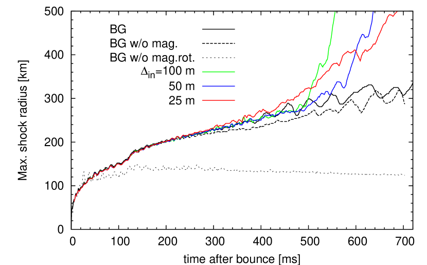
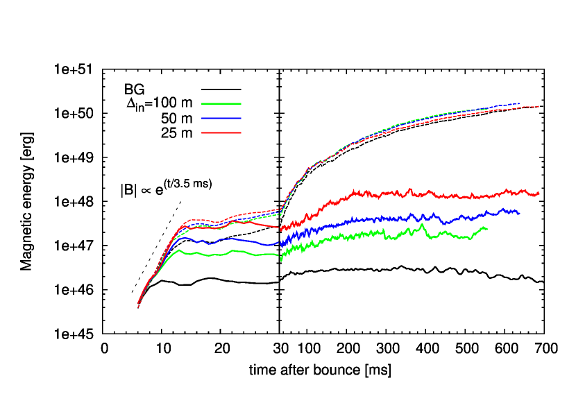
Figure 1.— Top panel: Evolutions of the maximum shock radii. Bottom panel: Evolutions of the magnetic energies integrated over $50\leq(r/$km$)\leq 500$ for the poloidal component (solid lines) and toroidal component.

As can be seen from the top panel of Figure 1, the MRI runs obtain more rapid increases of the maximum shock radius compared with the BG run. The evolutions of the diagnostic explosion energy, which is the energy integrated over the fluid elements that move outwards with positive energies, also indicate that the shock expansion leads to explosions in the MRI runs but not in the BG run (see Fig 2). While the shock radius grows fastest in the L-MRI run, the H-MRI run is likely to give the strongest explosion. As discussed bellow, we found that this is a consequence of efficient angular momentum transfer by larger saturation fields obtained in higher resolution runs.

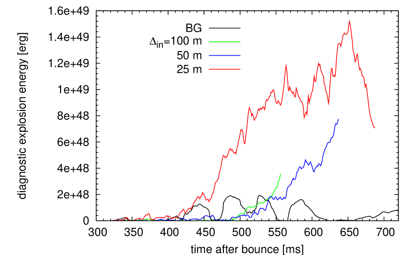
Figure 2.— Evolutions of the diagnostic explosion energies defined in the text.

Figure 3 displays the color maps of plasma beta, $\beta=8\pi p/B^{2}$, and radial velocity for all simulations at 555 ms after bounce. One can recognize a qualitative change in dynamics between the BG run and the L-MRI run: a low-$\beta$ region around the pole extend further and mass ejection instead of accretion occurs in the L-MRI run. Interestingly, however, low-$\beta$ region shrinks again with the further improvement of resolution. As a result the jet disappears and mass accretion occurs again around the pole in the M-MRI and H-MRI runs. On the other hand, mass ejection around mid-latitude becomes more prominent in H-MRI run (compare panel (b) and (d) of Figure 3). Although this mid-latitude ejection is slower than the polar ejection observed in the L-MRI run, the former results in a larger explosion energy as seen in Figure 2, since the amount of ejected mass is larger. Note that panel (d) indicates that the mid-latitude ejection is not powered by magnetic pressure, since its plasma beta is $\sim 10$–1000.

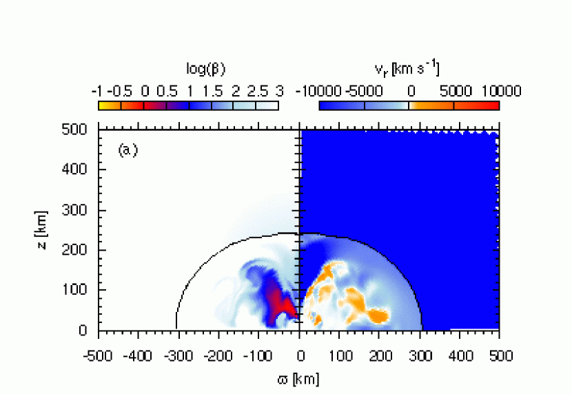
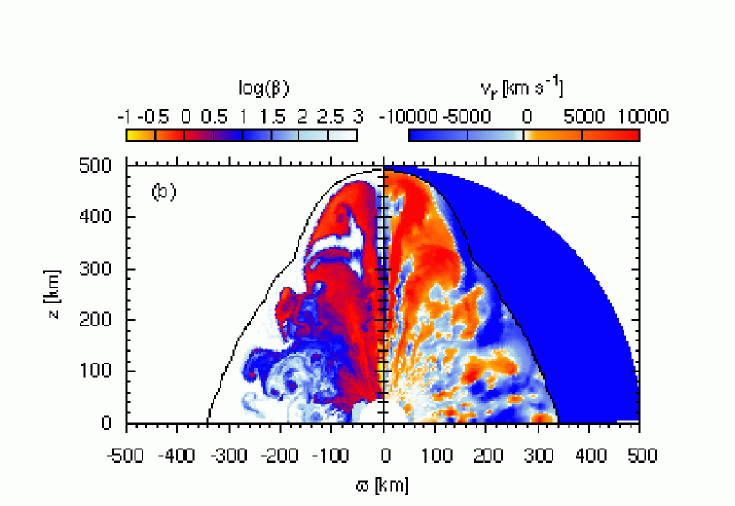
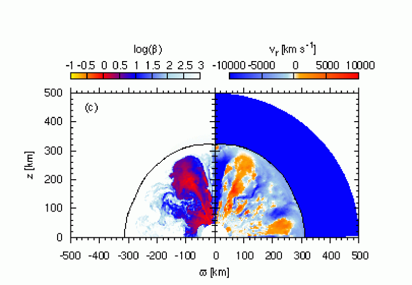
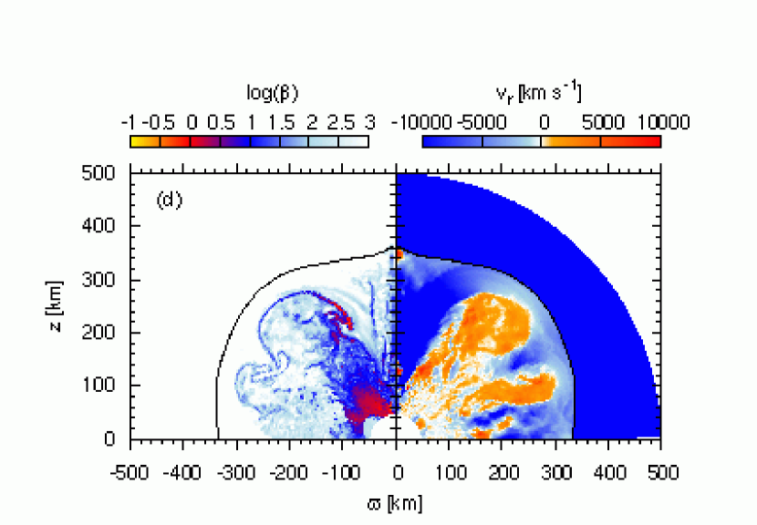
Figure 3.— Color maps of plasma beta (the left half) and radial velocity magnitude (the right half), and the contour of the shock surfaces (black line) at 555 ms after bounce for BG run (a), L-MRI run (b), M-MRI run (c), and H-MRI run (d).

The comparison between the advection timescale, $\tau_{\textrm{a}}$, during which matter traverses the gain region, and the heating timescale, $\tau_{\textrm{h}}$, within which matter gains enough energy to overcome gravity, is one of the rough measure to judge whether the neutrino heating plays an important role in driving explosion (Thompson, 2000). Following Dolence et al. (2013), we define the advection timescale as

$$\tau_{\textrm{a}}=\int^{R_{\textrm{gain}}}_{R_{\textrm{sh}}}\frac{dr}{\langle\langle v_{r}\rangle\rangle},$$ (7)

where the double angle bracket denotes that the solid-angle average and time average over the interval of 10 ms are taken. $R_{\textrm{sh}}$ is taken as the mean shock radius, whereas $R_{\textrm{gain}}$ is defined as the innermost radius at which the solid-angle averaged net heating is positive. The heating timescale is defined as

$$\tau_{\textrm{h}}=\frac{4\pi\int^{R_{\textrm{gain}}}_{R_{\textrm{sh}}}\langle e+\frac{\rho v^{2}}{2}+\frac{B^{2}}{8\pi}+\rho\Phi\rangle r^{2}dr}{4\pi\int^{R_{\textrm{gain}}}_{R_{\textrm{sh}}}\langle Q_{E}^{\textrm{em}}+Q_{E}^{\textrm{abs}}\rangle r^{2}dr},$$ (8)

where the angle brackets denote that the solid-angle average is taken. Panel (a) of Figure 4 displays the temporal variations of $\tau_{\textrm{a}}/\tau_{\textrm{h}}$. It is shown that the neutrino heating is important in all numerical runs and that the heating efficiency is higher in the MRI runs than in the BG run. While the L-MRI and M-MRI runs have similar ratios of $\tau_{\textrm{a}}/\tau_{\textrm{h}}$, the H-MRI run has much larger ratio after $\sim 400$ ms, suggesting that the mid-latitude mass ejection observed in the H-MRI run (panel (d) of Figure 3) is driven by neutrino heating.

We think that the high $\tau_{\textrm{a}}/\tau_{\textrm{h}}$ in the H-MRI run is caused by an efficient angular momentum transfer. In fact, panel (b) of Figure 4 shows that the angular momentum per unit mass in the H-MRI run is larger than that in the L-MRI run for $\theta\gtrsim 25^{\circ}$, and vice versa for $\theta\lesssim 25^{\circ}$, which is probably a consequence of more efficient angular momentum transfer in H-MRI run. The rate of angular momentum transfer is proportional to the product of the poloidal and toroidal components of magnetic field. Although the saturation level of the toroidal component is similar among all the simulations presented in this letter, the larger poloidal field at saturation in the H-MRI run than in the other runs (bottom panel of Figure 1) makes angular momentum transfer more efficient. This then leads to the widening of the heating region at low latitudes in the same model due to the extra-rotational support (compare the bottom panels of Figure 4.) As a consequence, the advection timescale becomes long, and thus the heating efficiency gets higher. Although the heating region is thicker around the pole in the L-MRI run than in the H-MRI run, this contributes little to the volume integrated heating rate because of the small mass in the region.

The fact that the mass ejection around the pole in the L-MRI run turns to the mass accretion in higher resolution run (see Figure 3) could be also accounted for by the efficiency of angular momentum transfer. Since the rotational support around the pole is weaker for the higher resolution runs, matter accretes more easily. This argument seems to contradict the fact that the mass accretion in the BG run turns to the mass ejection in the L-MRI run in the first place. The point here is that there is a trade-off between the gain in the magnetic stress and the loss in the centrifugal support.

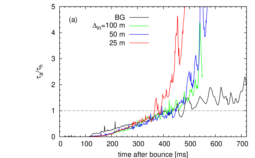
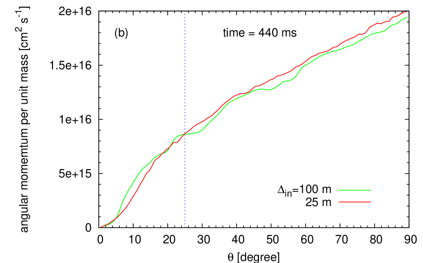
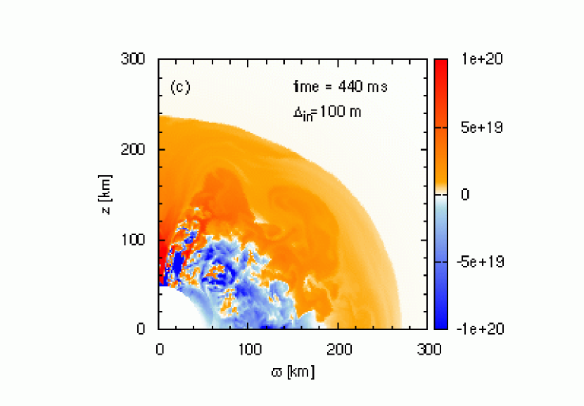
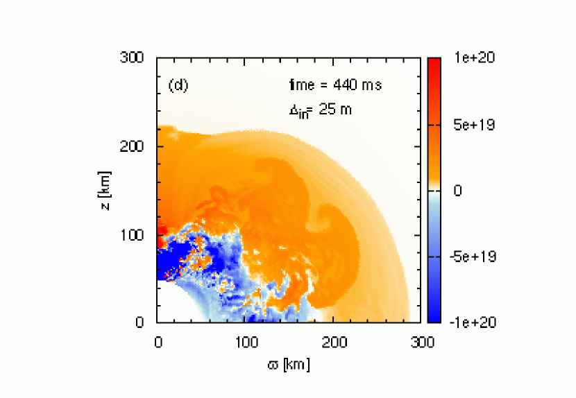
Figure 4.— (a):Evolutions of the ratio of the advection timescale to heating timescale, whose definitions are given in the text. (b): Angular distributions of the radially averaged angular momentum per unit mass at 440 ms after bounce for L-MRI run (green line) and H-MRI run (red line). Bottom panels: Color maps of the net heating rate per unit mass at 440 ms after bounce for L-MRI run (c) and H-MRI run (d).

4. Discussion and Conclusion

We conducted two dimensional high-resolution global MHD simulations of CCSNe, assuming that a massive star core is rather weakly magnetized and rapidly rotating prior to collapse. Taking neutrino heating and cooling into account approximately, we followed the evolutions long after core bounce and studied the dynamical consequences of MRI. We found that the magnetic field amplified by MRI indeed affects the dynamics thereafter substantially enhances the explosion. In fact, it efficiently transfers angular momentum from high to low latitudes and expands the heating region at low latitudes not by magnetic stress but by centrifugal force. This then enhances the heating efficiency and leads to explosion. This is a new explosion mechanism, which we expect to work generally in weakly magnetized, rapidly rotating stellar cores. In fact, although even our highest-resolution run has not yet achieved numerical convergence particularly in the sub-dominant poloidal component, further improvement of resolution would result in more efficient angular momentum transfer and thus in higher neutrino heating, which would make shock revival by neutrino heating even easier.

Previous simulations of weakly magnetized, rapidly-rotating cores by Burrows et al. (2007) and Takiwaki et al. (2009) found magneto-driven jets formed along the rotation axis, which are analogous to what we found in the L-MRI run. Since the spacial resolution in Burrows et al. (2007) is in between our BG and L-MRI runs, where the transition from mass accretion to ejection occurs near the pole, their results do not contradict ours. What they observed may be an artifact by insufficient numerical resolutions as demonstrated in the current study. Although Burrows et al. (2007) claimed that the neutrino heating is subdominant (contributing 10–25 % to the explosion energy), our simulations indicate that it is actually predominant. The spacial resolution in Takiwaki et al. (2009) is coarser than our BG run. The reason for the jet formations in their simulations may be because they assumed strong differential rotation prior to collapse with a typical scale height of 100 km in the $\varpi$ direction.

The diagnostic explosion energy obtained in our highest resolution simulation (H-MRI run) is $\sim 10^{49}$ erg, which is far smaller than the canonical value, $10^{51}$ erg. It should be noted that the shock front reaches only the radius of 500 km at the end of the simulation. It is way too early to estimate the final value of the explosion energy, since it may increase as the shock front propagates outward. Further improvement of the spacial resolution may also increase the explosion energy, since more efficient angular momentum transfer is expected. Moreover, the neutrino luminosity of $10^{52}$erg s^-1 assumed in this study may be a bit too low. In fact, a recent simulation by Bruenn et al. (2013) obtained $\nu_{e}$/$\bar{\nu_{e}}$ of several $10^{52}$erg s^-1 for the first 200 ms after bounce, which decreases to $\approx 10^{52}$erg s^-1 only later at $\sim 700$ ms after bounce. Larger neutrino luminosities will certainly result in larger explosion energies. Apart from the quantitative estimation of the explosion energy, what is most important here is the finding that even a weak magnetic field added to a rapidly rotating core may make the neutrino-driven explosion easier.

References

- Akiyama et al. (2003) Akiyama, S., Wheeler, J. C., Meier, D. L., & Lichtenstadt, I. 2003, ApJ, 584, 954
- Balbus & Hawley (1991) Balbus, S. A., & Hawley, J. F. 1991, ApJ, 376, 214
- Bruenn et al. (2013) Bruenn, S. W., Mezzacappa, A., Hix, W. R., et al. 2013, ApJ, 767, L6
- Burrows et al. (2007) Burrows, A., Dessart, L., Livne, E., Ott, C. D., & Murphy, J. 2007, ApJ, 664, 416
- Dolence et al. (2013) Dolence, J. C., Burrows, A., Murphy, J. W., & Nordhaus, J. 2013, ApJ, 765, 110
- Ferrario & Wickramasinghe (2006) Ferrario, L. & Wickramasinghe, D. T. 2006, Mon. Not. Astron. Soc., 367, 1323
- Heger et al. (2005) Heger, A., Woosley, S. E., & Spruit, H. C. 2005, ApJ, 626, 350
- Janka (2001) Janka, H.-T. 2001, A&A, 368, 527
- Liebendörfer (2005) Liebendörfer, M. 2005, ApJ, 633, 1042
- Masada et al. (2012) Masada, Y., Takiwaki, T., Kotake, K., & Sano, T. 2012, ApJ, 759, 110
- Moiseenko et al. (2006) Moiseenko, S. G., Bisnovatyi-Kogan, G. S., & Ardeljan, N. V. 2006, MNRAS, 310, 501
- Müller et al. (2012) Müller, B., Janka, H.-T., & Marek, A. 2012, ApJ, 756, 84
- Murphy et al. (2009) Murphy, J. W., Ott, C. D., & Burrows, A. 2009, ApJ, 707, 1173
- Obergaulinger et al. (2006) Obergaulinger, M., Aloy, M. A., & Müller, E. 2006, A&A, 450, 1107
- Obergaulinger et al. (2009) Obergaulinger, M., Cerdá-Durán, P., Müller, E., & Aloy, M. A. 2009, A&A, 498, 241
- Ramírez-Agudelo et al. (2013) Ramírez-Agudelo, O. H., Simón-Díaz, S., Sana, H., et al. 2013, A&A, 560, A29
- Shen et al. (1998a) Shen, H., Toki, H., Oyamatsu, K., & Sumiyoshi, K. 1998a, Nuclear Physics A, 637, 435
- Shen et al. (1998b) Shen, H., Toki, H., Oyamatsu, K., & Sumiyoshi, K. 1998b, Progress of Theoretical Physics, 100, 1013
- Sawai et al. (2013a) Sawai, H., Yamada, S., Kotake, K., & Suzuki, H. 2013, ApJ, 764, 10
- Sawai et al. (2013b) Sawai, H., Yamada, S., & Suzuki, H. 2013, ApJ, 770, L19
- Shibata et al. (2006) Shibata, M., Liu, Y. T., Shapiro, S. L., & Stephens, B. C. 2006, Phys. Rev. D, 74, 104026
- Suwa et al. (2010) Suwa, Y., Kotake, K., Takiwaki, T., et al. 2010, PASJ, 62, L49
- Takiwaki et al. (2009) Takiwaki, T., Kotake, K., & Sato, K. 2009, ApJ, 691, 1360
- Thompson (2000) Thompson, C. 2000, ApJ, 534, 915
- Wade et al. (2012) Wade, G. A., Grunhut, J., Gräfener, G., et al. 2012, MNRAS, 419, 2459
- Woosley & Heger (2006) Woosley, S. E., & Heger, A. 2006, ApJ, 637, 914
- Yamada & Sawai (2004) Yamada, S., & Sawai, H. 2004, ApJ, 608, 907