Large-deviation properties of resilience of transportation networks

Abstract

Distributions of the resilience of transport networks are studied numerically, in particular the large-deviation tails. Thus, not only typical quantities like average or variance but the distributions over the (almost) full support can be studied. For a proof of principle, a simple transport model based on the edge-betweenness and three abstract yet widely studied random network ensembles are considered here: Erdős-Rényi random networks with finite connectivity, small world networks and spatial networks embedded in a two-dimensional plane. Using specific numerical large-deviation techniques, probability densities as small as $10^{-80}$ are obtained here. This allows to study typical but also the most and the least resilient networks. The resulting distributions fulfill the mathematical large-deviation principle, i.e., can be well described by rate functions in the thermodynamic limit. The analysis of the limiting rate function reveals that the resilience follows an exponential distribution almost everywhere. An analysis of the structure of the network shows that the most-resilient networks can be obtained, as a rule of thumb, by minimizing the diameter of a network. Also, trivially, by including more links a network can typically be made more resilient. On the other hand, the least-resilient networks are very rare and characterized by one (or few) small core(s) to which all other nodes are connected. In total, the spatial network ensemble turns out to be most suitable for obtaining and studying resilience of real mostly finite-dimensional networks. Studying this ensemble in combination with the presented large-deviation approach for more realistic, in particular dynamic transport networks appears to be very promising.

1 Introduction

Transportation networks albert2002review ; newman2003review ; newman_book2006 ; dorogovtsev_book2006 ; cohen_book2010 ; barrat_book2012 , like computer networks, railway systems, water pipelines or energy grids, are ubiquitous in highly technological societies. Since the well functioning of these societies depends heavily on transportation networks, large-scale (cascading) failure are in particular threatening. Previous work on cascading failures in networks have often analyzed the occurrence of past failures chen2005 ; bao2009b or studied phase transitions, as a function of some network parameter, from a resilient to a failure phase deArcangelis1985 ; crucitti2004 ; dobson2007 ; bao2009 . In this work we are concerned always with the case of a design in such a way that a failure is prevented, i.e., resilient networks, the typical task of an engineer. In particular, we are interested on how to make a network fail-safe against the failure of one link by including enough, but as small as possible, backup capacity, such that a cascading failure is prevented (called “$N-1$ criterion” for power transmission). To gain a fundamental understanding of the problem, no real-world networks are studied here. Instead, this study is performed for three different network ensembles, two of them are highly relevant for transport processes in spatial settings, another simple model is included for comparison. Here, the behavior over the range of (almost) each complete ensemble is addressed, this means in particular the properties of typical as well as extremely resilient and extremely weak networks are investigated. Namely, the distribution of backup capacities is obtained for almost the complete support, for backup capacities which appear about $10^{-80}$ less likely than in typical networks. This requires to apply special but simple numerical importance-sampling techniques, as explained in section 5, to obtain the large-deviation properties of the networks.

For many problems in science and in statistics, the large-deviation properties play an important role denHollander2000 ; dembo2010 . Only for few cases analytical results can be obtained. Thus, most problems have to be studied by numerical simulations practical_guide2009 , in particular by Monte Carlo (MC) techniques newman1999 ; landau2000 . Classically, MC simulations have been applied to ensembles of random systems in the following way: For a finite number of independently drawn instances from the ensemble, arbitrary properties of these instances have been calculated using MC simulations. Later, it has been noticed that MC simulations can be used via introducing an artificial “temperature” to sample the random ensemble such that the large-deviation properties of the (almost) full ensemble can be obtained align2002 . The results are re-weighted in a way that the results for the original quenched ensemble are obtained. In this way, the large-deviation properties of the distribution of alignment scores for protein comparison were studied align2002 ; align_long2007 ; newberg2008 , which is of importance to calculate the significance of results of protein-data-base queries durbin2006 .

Motivated by these results, similar approaches have been applied to other problems like the distribution of the number of components of Erdős-Rényi (ER) random networks rare-graphs2004 , the size of the largest components of ER random networks and of two-dimensional grids largest-2011 , the partition function of Potts models partition2005 , the distribution of ground-state energies of spin glasses pe_sk2006 and of directed polymers in random media monthus2006 , the distribution of Lee–-Yang zeros for spin glasses matsuda2008 , the distribution of success probabilities of error-correcting codes iba2008 , the distribution of free energies of RNA secondary structures rnaFreeDistr2010 , and some large-deviation properties of random matrices driscoll2007 ; saito2010 .

To the knowledge of the author, no corresponding study has been performed to obtain the large-deviation properties of transport networks, in particular of failure-resilient networks. Here, the large-deviation approach is applied to a simple yet often used transport model on three standard random network ensembles. Thus, this work serves in particular as a proof of principle that measuring large-deviation properties of transport networks is possible and allows one to obtain useful insight. This shows that similar approaches should be applicable to more complex transport networks, e.g., dynamic networks of oscillators as used to study energy grids filatrella2008 ; rohden2012 .

The remainder of the paper is organized as follows. First, in Sec. 2, the different network ensembles under scrutiny are presented. Then, the backup capacity is introduced, which is used to describe how resilient a network is. In Sec. 4 a couple of test simulations are presented, which explore the concept of the backup capacity. In the following section, the large-deviation approach is presented. Within the main Sec. 6, all results are given. The paper is closed by a summary and a discussion.

2 Network Ensembles

This work is about the resilience of network ensembles, since such ensembles are used often in theoretical studies about various network properties. This type of approach is different from the question how, e.g., the most resilient network for a given set of nodes and real-space positions looks like. For such a setup the notion of an ensemble makes less sense and is thus not covered in this work. Also no existing networks are studied empirically here since that would be beyond the scope of the work. Nevertheless, the present approach allows to gain insights about the behavior of typical and atypical network instances, leading to general design principles for resilient networks.

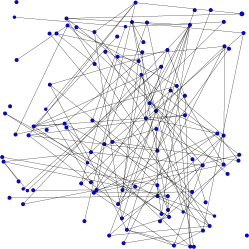
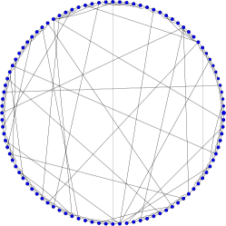
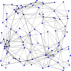
Figure 1: Three different ensembles are treated. For each ensemble, a sample network with $N=100$ nodes is shown: Erdős-Rényi random networks (top, with randomly placed nodes), small-world networks (middle) and two-dimensional spatial networks (bottom).

The most simple type of random networks is the Erdős-Rényi (ER) network ensemble erdoes1960 . It makes no assumption about the topology of the network, i.e., in particular it exhibits no spacial structure, see Fig. 1 (top). Thus, it is ideally suited for comparison with more complex network ensembles as well as single network instances to see what effect the structures of these more complex networks have regarding their behavior. To create an ER random network, one starts with an empty network of $N$ nodes. For each pair $i,j$ of nodes, with some given probability $p_{ij}^{\rm ER}$ the link $\{i,j\}$ is added to the network. Here,

$$p_{ij}^{\rm ER}=c/(N-1)$$ (1)

is chosen such that, on average, each node has $c$ connections. Nevertheless, all possible networks have a nonzero (although sometimes quite small) probability, even the complete (fully connected) as well as the empty network. Since ER random networks have a minimum amount of structure, they often serve as a suitable null model when comparing to other ensembles of random networks.

Next, a widely studied model of networks is considered here, the small-world (SW) ensemble watts1998 ; amaral2000 ; barrat2001 . This ensemble was found, e.g., to represent the U.S. power grid well watts1998 ; amaral2000 ; motter2002 and was used for modelling other transport networks as well bao2009 . For this model, in a first step $N$ nodes are distributed on a ring and connected with their direct and second-nearest neighbors. Thus, each node has four links. Next, for each existing link, with probability $p$ (here $p=0.1$) it is disconnected at one terminal node and reconnected with a completely randomly chosen node, hence keeping the average number of links per node. Thus, for $p\to 1$ the SW networks become more similar to a modified ER ensemble where the average number of neighbors is $c=4$ and where the actual number of links does not fluctuate. For $p$ small, this results in a mixture of many local short-range and few long-range links, see Fig. 1 (middle), which is a key characteristics of many existing real-world networks. Note that for easy comparison between different network models, $c=4$ was chosen here for the ER ensemble, such that all network ensembles have the same average number of neighbors.

Since many existing transport networks are embedded on a two-dimensional (earth) surface, also a spatial (two-dimensional) model barthelemy2011 is included in the present study, which exhibits even more spatial structure than the SW ensemble. Here, $N$ nodes are distributed randomly with uniform weight in a $[0,1]^{2}$-plane. Afterward, for each pair $i,j$ of nodes, with probability

$$p_{ij}^{\rm sp}=f\cdot(1+\sqrt{N\pi}d_{ij}/\alpha)^{-\alpha}$$ (2)

the link $\{i,j\}$ is added to the network, where $d_{ij}$ is the Euclidean distance between nodes $i,j$. A sample network is shown in Fig. 1 (bottom). Here, values $f=0.95$ and $\alpha=3$ are chosen, which results also in an average number of neighbors close to $4$. Note that several variants of spatial networks exist in the literature. Although the model appears to be in particular useful for surface-embedded transportation networks, it is so far less established than the SW model, so the many results for the SW model are included here as well.

3 Resilience

The quantity to describe the resilience of a network against a failure leading to cascading failures is based on a rather simple (i.e., not time-dependent) yet established quantity to measure loads in transport networks motter2002 ; motter2004 ; bao2009 . The loads are given by the assumption that for each pair $i,j$ of nodes, a unit one of some quantity has to be transported between $i,j$. This requires the network to be connected, i.e., to consist of a single connected component. For the above random ensembles it means that they are restricted to the subset of connected network instances. For the SW model and the spatial model basically all network instances are connected using the given parameters, while for the ER model typically only a small fraction of networks is connected (37% for $N=50$, 15% for $N=100$, 2.5% for $N=200$ and 0.005% for $N=400$). Note that the sampling used here, see Sec. 5, ensures that only connected networks are sampled.

For the transport between any pair $i,j$ of nodes the shortest path is chosen (if several shortest paths exist, the transportation is divided equally among the different paths). This is performed for all pairs of nodes, which are connected in the network. The actual load $l_{i,j}$ for an link $e=\{i,j\}$ is the total number of (possibly sums of fractional) shortest paths which run through the link. Hence, the load is equal to the well known edge-betweenness, which can be calculated conveniently using a fast algorithm newman2001shortest-path .

Now, the backup capacity $c_{\rm b}$ is defined. For this purpose, the link $e_{\max}={\rm argmax}_{\{i,j\}}\,l_{i,j}$ exhibiting the highest load is removed from the network. Next, all loads are recalculated, resulting in load values $\{\tilde{l}_{i,j}\}$ of the modified network. The backup capacity is defined as the highest increment in the load, i.e.,

$$c_{\rm b}=\max_{\{i,j\}}(\tilde{l}_{i,j}-l_{i,j})\,.$$ (3)

If the network is disconnected by the removal of $e_{\max}$, $c_{\rm b}=\infty$ is chosen, i.e., such networks are actually disregarded as well. The (or one) link which exhibits the maximum increase in load is denoted here by $e_{\rm incr-max}$. Note that in some link the load will actually decrease, but that is no problem for the definition. Hence, the backup capacity represents a rough and rather safe estimate of how much the capacities have to be chosen above the actual load values to make the transportation network resilient against the failure of one link.

4 Test simulations

Figure 2: Scatter plot of the full backup capacity $c_{\rm b}^{\rm full}$, which is optimized over the removal of every link, one at a time, as a function of actually used backup capacity $c_{\rm b}$ (where only the link with the largest load is removed), for small-world networks with $N=100$ and $p=0.1$.

To verify whether concentrating on the removal of the link with the largest load (leading to backup capacity $c_{\rm b}$) is justified, simulations were performed such that for each network the necessary backup capacity was also maximized over the single-link removal of all links, resulting in a maximum backup capacity $c_{\rm b}^{\rm full}$. Clearly, $c_{\rm b}^{\rm full}\geq c_{\rm b}$ holds for any network. In Fig. 2, results for small-world networks with $N=100$ nodes and rewiring probability $p=0.1$ are displayed, the results for other network ensembles look similar. As visible, there is a strong correlation between the full backup capacity $c_{\rm b}^{\rm full}$ and the actually used backup capacity $c_{\rm b}$. A linear correlation coefficient $0.85$ was found. In fact, for about 1/3 of all networks, both are exactly equal and for more than 90% $c_{\rm b}^{\rm full}\leq 2c_{\rm b}$ holds. Hence, due to the strong correlation, when optimizing the network topology with respect $c_{\rm b}$ one will also obtain very efficient networks with respect to $c_{\rm b}^{\rm full}$.

Figure 3: Probability $P_{\rm cascade}$ of a cascade which disconnects the network as a function of the fraction $f_{\rm b}$ of the backup capacity added to the link capacities. For small-world networks with different sizes $N=20$, $N=50$, $N=100$ and $p=0.1$.

Thus, for best efficiency, for the main simulations the above quantity $c_{\rm b}$ was evaluated, i.e. only one link was removed and the load recalculated. Nevertheless, in principle one is interested in global events, i.e., in cascading failures crucitti2004 . The basic assumption is that when the backup capacity is not sufficient, a cascading failure will be triggered frequently. This assumption was also checked explicitly in this work for the sample setup of SW networks ($p=0.1$): After the calculation of the backup capacity $c_{\rm b}$ the capacity of every link was increased by the amount $f_{b}c_{\rm b}$, where $f_{b}$ is a factor in the range $[0,2.5]$, except for the link $e_{\rm incr-max}$ which exhibits the largest load increase after the initial removal. For this link the capacity is increased only by $c_{\rm p}-\epsilon$, where $\epsilon>0$. Thus, this link will for sure fail next with the recalculated load distribution since the capacity is not sufficient. Thus it has to be removed as well and the load distribution has to be recalculated again. Now even more links may fail. This process is repeated, until no more links fail, i.e., the network is able to redistribute the load, or until a cascade of failures result in the network breaking apart, i.e. a complete breakdown. In Fig. 3, the probability $P_{\rm cascade}$ of a cascading failure leading to a network breakdown is shown as a function of $f_{b}$. Clearly, for $f_{b}<1$ almost all failures trigger a network breakdown. On the other hand, when increasing $f_{b}$ cascading failures become less likely. Hence, it is justified to calculate just the backup capacity $c_{\rm b}$, involving only two calculations of the load distribution, to learn about the resilience of the network against an event leading to a cascading failure.

5 Simulation and reweighting method

To determine the distribution $P(c_{\rm b})$ for any measurable quantity $c_{\rm b}$, here denoting the backup capacity of a network, simple sampling is straightforward: One generates a certain number $K$ of network samples and obtains $c_{\rm b}(G)$ for each sample $G$. This means each network $G$ will appear with its natural ensemble probability $Q(G)$. The probability to measure a value of $c_{\rm b}$ is given by

$$P(c_{\rm b})=\sum_{G}Q(G)\delta_{c_{\rm b}(G),c_{\rm b}}$$ (4)

Therefore, by calculating a histogram of the values for $c_{\rm b}$, a good estimation for $P(c_{\rm b})$ is obtained. Nevertheless, $P(c_{\rm b})$ can only be measured in a regime where $P(c_{\rm b})$ is relatively large, about $P(c_{\rm b})>1/K$. Unfortunately, the distribution decreases for many systems exponentially fast in the system size $N$ when moving away from its typical (peak) value. This means, even for moderate system sizes $N$, the distribution will be unknown on almost its complete support.

To estimate $P(c_{\rm b})$ for a much larger range, even possibly on the full support of $P(c_{\rm b})$, where probabilities smaller than $10^{-10}$ may appear, a different approach is used align2002 . For self-containedness, the method is outlined subsequently. The basic idea is to use an additional Boltzmann factor $\exp(-c_{\rm b}(G)/T)$, $T$ being a “temperature” parameter, in the following manner: A Markov-chain MC simulation newman1999 ; landau2000 is performed, where in each step $t$ from the current network $G(t)$ a candidate network $G^{*}$ is created: A node $i$ of the current network is selected randomly, with uniform weight $1/N$, and all adjacent links are deleted. For all feasible links $\{i,j\}$, the link is added with a weight corresponding to the natural weight $Q(G)$, e.g., with probability $c/(N-1)$ for ER random networks. For SW and spatial networks it is done correspondingly, see Sec. 2. Next, it is checked whether network $G^{*}$ is connected, i.e., consists of one single connected component, because only for a connected network the backup capacity is defined. If $G^{*}$ is not connected, it is rejected, i.e. $G(t+1)=G(t)$. Note that it has to be made sure that the initial network is connected. This was achieved by generating candidates for the initial network until a connected instance was found.

If the candidate network is connected, the backup capacity $c_{\rm b}(G^{*})$ is calculated. Finally, the candidate network is accepted, ($G(t+1)=G^{*}$) with the Metropolis probability

$$p_{\rm Met}=\min\left\{1,e^{-[c_{\rm b}(G^{*})-c_{\rm b}(G(t))]/T}\right\}\,.$$ (5)

Otherwise the candidate network is also rejected ($G(t+1)=G(t)$). By construction, the algorithm fulfills detailed balance. Clearly the algorithm is also ergodic, since within $N$ steps, each possible network may be constructed, in principle. Thus, in the limit of infinite long Markov chains, the distribution of networks will follow the probability

$$q_{T}(G)=\frac{1}{Z(T)}Q(G)e^{-c_{\rm b}(G)/T}\,,$$ (6)

where $Z(T)$ is the a priori unknown normalization factor.

The distribution for $c_{\rm b}$ at temperature $T$ is given by

$$P_{T}(c_{\rm b}) = \sum_{G}q_{T}(G)\delta_{c_{\rm b}(G),c_{\rm b}}$$

$$\stackrel{{\scriptstyle(\ref{eq:qT})}}{{=}} \frac{1}{Z(T)}\sum_{G}Q(G)e^{-c_{\rm b}(G)/T}\delta_{c_{\rm b}(G),c_{\rm b}}$$

$$= \frac{e^{-c_{\rm b}/T}}{Z(T)}\sum_{G}Q(G)\delta_{c_{\rm b}(G),c_{\rm b}}$$

$$\stackrel{{\scriptstyle(\ref{eq:PS})}}{{=}} \frac{e^{-c_{\rm b}/T}}{Z(T)}P(c_{\rm b})$$

$$\Rightarrow\quad P(c_{\rm b}) = e^{c_{\rm b}/T}Z(T)P_{T}(c_{\rm b})$$ (7)

Hence, the target distribution $P(c_{\rm b})$ can be estimated, up to a normalization constant $Z(T)$, from sampling at finite temperature $T$. For each temperature, a specific range of the distribution $P(c_{\rm b})$ will be sampled: Using a positive temperature allows to sample the region of a distribution left to its peak (values smaller than the typical value), while negative temperatures are used to access the right tail. Temperatures of large absolute value will cause a sampling of the distribution close to its typical value, while temperatures of small absolute value are used to access the tails of the distribution. Hence, by choosing a suitable set of temperatures, $P(c_{\rm b})$ can be measured over a large range, possibly on its full support.

The normalization constants $Z(T)$ can easily be obtained by including a histogram obtained from simple sampling, which corresponds to temperature $T=\pm\infty$, which means $Z\approx 1$ (within numerical accuracy). Using suitably chosen temperatures $T_{+1}$, $T_{-1}$, one measures histograms which overlap with the simple sampling histogram on its left and right border, respectively. Then the corresponding normalization constants $Z(T_{\pm 1})$ can be obtained by the requirement that after rescaling the histograms according to (7), they must agree in the overlapping regions with the simple sampling histogram within error bars. This means, the histograms are “glued” together, similar to the multi-histogram approach of Ferrenberg and Swendsen ferrenberg1989 . In the same manner, the range of covered $c_{\rm b}$ values can be extended iteratively to the left and to the right by choosing additional suitable temperatures $T_{\pm 2},T_{\pm 3},\ldots$ and gluing the resulting histograms one to the other. A pedagogical explanation and examples of this procedure can be found in Ref. align_book .

In order to obtain the correct result, the MC simulations must be equilibrated. The equilibration of the simulation can be monitored by starting with two different initial networks, respectively:

• First an unbiased random network is taken, which means that the measure of interest is close to its typical value.

• Second, one uses a very atypical network, e.g., a fully connected network.

In any case, for the two different initial conditions, the evolution of $c_{\rm b}(G(t))$ will approach from two different extremes, which allows for a simple equilibration test: equilibration is achieved if the measured values of $c_{\rm b}$ agree within the range of fluctuations. For the simulations performed in this work, equilibration was achieved always within 200 Monte Carlo sweeps (i.e., $200*N$ Monte Carlo steps).

6 Results

Simulations where performed for ER, SW and spatial networks. For each type, several number of nodes were considered, to study finite-size effects. The evaluation of the backup capacity is rather involved, compared, e.g., to past large-deviation studies of the largest component of networks largest-2011 . Thus, the largest networks under scrutiny here exhibit $N=400$ nodes. Nevertheless, many existing transportation networks are of similar size.

Figure 4: Probability distribution $P(c_{\rm b})$ for the backup capacity $c_{\rm b}$, for small-world networks ($p=0.1$) with different sizes $N=50$, $100$, $200$ and $400$. Standard error bars are at most of order of symbol size. The line shows a fit of the tail ($c_{\rm b}\geq 20000$) of the $N=400$ data to an exponential ($a\exp({-c_{\rm b}/\tilde{c}})$, $a=2.4(1)\times 10^{-5}$, $\tilde{c}=1022(1)$). The inset enlarges the region near $c_{\rm b}=0$, the line being a guide to the eyes only.

Figure 4 shows the distribution of the backup capacity for almost the full support for the ensemble of SW networks. Note that probabilities as small as $10^{-22}$ are easily obtained which are clearly out of reach using conventional simulation techniques. Typical, very reliable and very unreliable networks are accessible using the large-deviation approach. Typical networks, near the peak of the distributions, exhibit a rather small backup capacity. Very unreliable networks, where the backup capacity has to be large to prevent cascading failures, are very rare and located in the tails of the distributions to the right. The tails of the distribution follow exponentials very well, as a fit to $a\exp({-c_{\rm b}/\tilde{c}})$ to the tail of the data for the largest networks revealed, resulting in $a=2.4(1)\times 10^{-5}$, $\tilde{c}=1022(1)$. Below a more detailed analysis via an extrapolation of the large-deviation rate function is given, supporting that the limiting distribution is exponential.

An inspection of the networks in the far tail of the distribution showed that the most unreliable networks have a quite special structure. They consist of a small core of connected nodes, e.g., a triangle of nodes in the simplest case, see Fig. 5. All remaining ($N-3$) nodes are connected, directly or indirectly, to one of two of these core nodes, roughly partitioned equally into two sets, i.e. about $N/2$ per set of nodes. This means, a large number of $(N/2)^{2}$ shortest-path connections runs from one set through a single link of the core to the other set. This single link exhibits the highest load, while the other core links are not used much. By removing this extreme-load link, the load is redistributed completely in the core, hence, increased by an amount of $\sim N^{2}/4$. Clearly, such networks are very rare by chance and rather special.

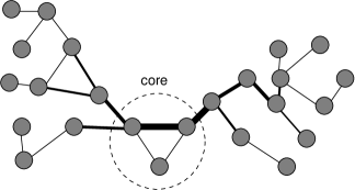
Figure 5: Network with highest backup capacity. Two large $O(N)$ subnetworks are connected trough a small core network (a triangle, here). The links with the highest loads are shown in bold. Removing the highest load from the core part results in an increase of the load through the other core links by an amount $N^{2}/4$.

On the other hand, there are also networks which have even a much more resilient structure than typical networks, since they require only a rather small backup capacity. They are located near the origin of the distribution and are also rather rare (probability $<10^{-9}$ for the largest case considered here). Below we will identify some structural network properties that make it very resilient.

The inset of Fig. 4 shows also that with increasing network size, the typical backup capacity, i.e., the location of the peak, grows. A more detailed study, also involving larger sizes which were studied by simple sampling, exhibits that the growth is linear (not shown here).

For comparison with the most simple network model, Erdős-Rényi (ER) random networks erdoes1960 , the corresponding results are shown in Fig. 6. The peak of the distribution again moves (linearly) to the right but is located relatively much further left compared to the SW case. Again an exponential fits the data well, now for almost over the full support.

Figure 6: Probability distribution $P(c_{\rm b})$ for the backup capacity $c_{\rm b}$, for Erdős-Rényi networks ($c=4$) with different sizes $N=50$, $100$, $200$ and $400$. Standard error bars are at most of order of symbol size. The line shows a fit over almost the full support ($c_{\rm b}\geq 5000$) of the $N=400$ data to an exponential ($a\exp({-c_{\rm b}/\tilde{c}})$, $a=0.015(2)$, $\tilde{c}=223(1)$). The inset enlarges the region near $c_{\rm b}=0$, lines being guides to the eyes only.

For comparison with the realistic spatial network model, the corresponding results are shown in Fig. 7. Typically, these networks are more resilient (smaller value of $c_{\rm b}$) than the SW networks, but less resilient than the ER model. Again, most of the distribution can be well fitted by an exponential.

Figure 7: Probability distribution $P(c_{\rm b})$ for the backup capacity, for spatial random networks ($\alpha=3$, $f=0.95$) with different sizes $N=50$, $N=100$, $N=200$ and $N=400$. Standard error bars are at most of order of symbol size. The line shows a fit over most of the support ($c_{\rm b}\geq 10000$) of the $N=400$ data to an exponential ($a\exp({-c_{\rm b}/\tilde{c}})$, $a=2.7(4)\times 10^{-5}$, $\tilde{c}=392(1)$). The inset enlarges the region near $c_{\rm b}=0$, lines being guides to the eyes only.

Comparing the insets of Fig. 4, 6 and 7, one observes that both ER random networks as well spatial random networks typically require a lower backup capacity compared to the SW model. Typical values of the backup capacity $c_{\rm b}$ for the ER model are located at small values ($c_{\rm b}\approx 40$ for $N=400$). The spatial networks are typically almost as resilient ($c_{\rm b}\approx 100$ for $N=400$). For the SW ensemble, typical networks need much larger backup capacity ($c_{\rm b}\approx 500$ for $N=400$). Correspondingly, large values of $c_{\rm b}$ are very unlikely for the ER ensemble (a density of $10^{-80}$ at $c_{\rm b}=40000$ for $N=400$) and quite unlikely for the spatial networks (a density of $10^{-50}$). For the SW model the density of $10^{-22}$ at rightmost tail is relatively larger. These quantitative differences in the large-deviation behavior are also reflected by the constants obtained by fitting an exponential to the tail of the distribution. The drop of the tail is strongest for the ER model, followed by the spatial ensemble and finally by the SW networks. Thus, the SW ensemble relatively favors less resilient networks compared to the other two ensembles. For the ER model this behavior is no big surprise because the ER model does not exhibit any spatial structure, allowing for arbitrary network topologies in particular many long-range links (equivalent to a high dimension of the system) which lead to a strong resilience. In particular the network where all pairs of nodes are directly connected (complete network) is contained in the ensemble, which is not possible for the SW ensemble because the average number of neighbours is fixed to 4.

On the other hand, the SW and the spatial model are both embedded in a low-dimensional structure, which might indicate that both should need larger backup capacities than the ER ensemble. Nevertheless, the spatial ensemble seems to be more similar to the ER networks with respect to the resilience. First, one should note that for the spatial networks in principle a complete network is possible (but even more unlikely than for ER random networks) in contrast to the SW ensemble. Second, the SW model exhibits indeed some long-range links, which can be used to decrease to overall load, hence the backup capacity. Nevertheless, by accident few of the long-range links will be very suitable for many of the shortest paths, acquiring much of the load, while many other long-range links carry only a small load. This “channeling effect” leads to a rather large backup capacity, thus a large load has to be rerouted after the failure. Opposite to this, for the spatial model, due to the distribution of the nodes in a two-dimensional plane, the total all-to-all traffic is distributed more over different paths, leading to a more uniform distribution of the load in the plane, in turn requiring less backup capacity.

Thus, using a true two-dimensional model, like the one applied here, appears from the present results the most meaningful approach within this field. This type of networks exhibit on the one hand spatial structure, as needed for most real-world applications, one the other hand, the resilience is typically, and also optimally, rather large. This is opposed to the SW model, which is often used to model power grids watts1998 ; amaral2000 ; motter2002 , but exhibits rather low resilience and is not embedded in a two-dimensional plane. Clearly, by increasing the fraction $p$ of randomized links, the SW model can be made more resilient, but that will render it much more similar to the ER model (without fluctuating number of links), but less finite-dimensional, i.e., less realistic.

Figure 8: Rate function $\phi$ for the rescaled backup capacity $r=c_{\rm b}/(N^{2}/4)$, for small-world networks ($p=0.1$) with different sizes $N=50$, $N=100$, $N=200$, $N=400$ and for the extrapolation $N\to\infty$. The line represents a power law fit to the extrapolated values. The inset shows a sample extrapolation (using a power law plus constant) for $r=0.4$.

Next, some information about the limiting distribution for large network sizes is obtained using the so-called rate function

$$\phi=-\frac{1}{N}\log P(c_{\rm b})$$ (8)

which is a standard quantity in large-deviation theory denHollander2000 ; touchette2009 . It displays the leading behavior under the assumption that away from the typical instances, the distribution decays exponentially fast in the system size, i.e., $P(c_{\rm b})\sim e^{-N\phi}$. In Fig. 8 the rate function as a function of the rescaled backup capacity $r=c_{\rm b}/(N^{2}/4)$ is shown for SW networks. This rescaling to $r$, motivated by the above finding about the most unresilient networks, ensures that the maximum of the support for the rate function is close to $r=1$. This allows for a comparison and extrapolation of the results for different sizes $N$. Just from looking at the data, the rate function seems to approach a limiting shape for larger networks.

To make this statement quantitatively precise, an extrapolation to $N\to\infty$ was performed in the following way: For selected fixed values of $r$, the rate function $\phi$ was considered as a function of the system size $N$ and fitted to a power law $\phi_{r}(N)=\phi_{r}^{\infty}+b_{r}N^{-c_{r}}$, which is a typical finite-size behavior found in statistical mechanics models. The inset of Fig. 8 shows the SW data and the resulting fit for the case $r=0.4$ (with $\phi_{0.4}^{\infty}=0.041(7)$, $b_{0.4}=1.9(6)$ and $c_{0.4}=0.72(9)$). The resulting extrapolated values $\phi_{r}^{\infty}$ are also displayed in Fig. 8 together with a fit to a power law $\phi_{r}^{\infty}=\alpha r^{\beta}$ ($\alpha=0.102(5)$,$\beta=0.97(10)$, i.e., close to a linear behavior), which is compatible with an exponential distribution ($\beta=1$) for the backup capacity in the thermodynamic limit. For the two other network types, the exponential nature of the tails of the distributions is even more obvious from the data shown in Figs. 6 and 7 directly, hence corresponding analyses of the rate function are omitted here. The fact that the data can be so well described by the rate function in the thermodynamic limit indicates that the problem studied here may be well accessible using analytical large-deviation approaches, which often are based on obtaining the rate function.

Finally, we want to understand the source of resilience in principle. Trivially, the higher the load in the most-loaded link, the more load has to be redistributed when this link is removed, i.e., the larger the needed backup capacity. More interesting it is to ask which network structures lead to resilient networks, without looking at the actual load values. Here, selected results are shown for the connection between the resilience and the number of links and, respectively, the diameter of a network.

First, the relationship of the resilience to the number of links is investigated. For this purpose, the $N=400$ networks obtained during the simulations at different temperatures $T$ were binned according to the number $n_{\rm e}$ of links. For the networks in each bin, the average backup capacity $c_{\rm b}$ was evaluated. The result is shown in Fig. 9 for the ER and the spatial random networks (for the SW ensemble, the number of edges does not vary). One sees that if only few links are available, the backup capacity is very large, which is meaningful, because having more links allows to distribute the load making a network more resilient. Interestingly, a sharp drop as a function of $n_{\rm e}$ is visible, looking like a phase transition. This drop appears for ER random networks at a smaller number of edges, which is meaningful, because ER networks exhibit no constraints, thus one has more “freedom” to arrange the links such that a high resilience can be obtained. Note that typical networks exhibit a very small backup capacity compared the the “high-backup capacity phase” in the left part of Fig. 9. Thus, this transition is not investigated more thoroughly here.

Figure 9: The average resilience $c_{\rm b}$ as a function of the number $n_{\rm e}$ of links for ER and spatial networks of size $N=400$.

Thus, including more edges leads, not surprisingly, to a higher resilience. Note that examples exist, where adding more links sometimes also decreases the stability of a network witthaut2012 . Anyway, for real networks, including more links leads almost always to larger costs (see also remarks below). Thus, it would be interesting to see how the resilience correlates with other topological measures of the network. For this purpose, a scatter plot of the backup capacity versus the diameter $d$ of a network (i.e., the longest among all shortest $i\leftrightarrow j$ paths) was recorded, see inset of Fig. 10 for the SW model. One can observe that large backup capacities go along with large diameters. Note that for the SW model, the differences in backup capacity can not originate from fluctuations of the number of edges. The positive relation between diameter and backup capacity can be seen even better in the main part of Fig. 10, where a binning of the networks with respect to $c_{\rm b}$ was performed (shown here just for typical and very resilient networks, i.e., small values of $c_{\rm b}$) and within each bin the average diameter was evaluated. Again, the positive correlation between diameter and backup capacity is visible, for all three network ensembles. In particular very small backup capacities, i.e, the most resilient graphs (which are not accessible using standard simple-sampling simulation approaches) are related to extremely small diameters. This shows that the diameter is a key quantity when considering and optimizing resilience of transport networks. Note that again ER ensemble and spatial networks are very similar behaving, although very different in definition. For the ER ensemble, for the most resilient instances obtained, an average diameter of $d\approx 2$ was measured, close to the value of $d=1$ of the complete network. Note that a complete network minus one edge has already diameter two. This shows that actually the most resilient networks were sampled during the simulations.

On the other hand, the SW ensemble exhibits for the same backup capacity a larger average diameter. This may occur on the first sight interesting since it allows for longer paths leading to the same resilience. On the other hand, this effect is only visible for slightly higher backup capacities. Therefore, in the region of extremely resilient networks, which are most interesting, the SW ensemble does not contribute at all, because such resilient networks do simple not exist there. Furthermore, extrapolating the SW data of $d$ by eye to small values of $c_{b}$ leads to small values of the diameter, which simply cannot be obtained in this ensemble.

Figure 10: The average diameter $d$ as a function of the resilience $c_{\rm b}$ for SW, ER and spatial networks of size $N=400$, in the range of small value of $c_{\rm b}$. The inset shows a scatter plot of the data for the entire range of backup capacities for the SW case.

Note finally that for real networks costs are an important issue. In order to observe how the resilience scales with the costs of a network, one would have to take into account the spatial length of the links and built upon that the costs which are a function of the number of links and their lengths. This is certainly beyond the scope of the current work which has its focus on abstract but standard and widespread network ensembles. Nevertheless, the general results as shown here will likely persist, in particular the strong correlation with the diameter of a network, which should be minimized for given costs.

7 Summary and outlook

The resilience of simple models of transportation networks against failures of highly-loaded links were studied here. For the random networks, three different ensembles were considered: The Erdős-Rényi ensemble is the most simple model for random networks, exhibiting no spatial structure at all, but serves well as a null model for comparison. Small-world networks are also very simple but are used often to model real-world transportation networks still rather well, like, e.g., energy grids. Finally, spatial networks are considered here, which are more sophisticated, but not well established. They might serve in the future as standard models for surface-based transportation.

To model the resilience against single-link failures (leading to cascading failures) the backup capacity is defined, which describes the amount of additional capacity, which one has to be included in the links to prevent a failure. The lower the backup capacity is, the more resilient, i.e., the better, is the structure of the network.

Here, a large-deviation approach was used to study the distribution of the backup capacity. Since the method allows to access a distribution (almost) on its complete support, one can study the scaling behavior not only of the typical and average but also of the best and the worst network instances. Networks leading to very small probability densities of the backup capacity such as $10^{-80}$ could be generated and studied with the correct weight via introducing a bias and reweighting the results for the analysis.

The main results are as follows: Trivially, by including more links, a network can be made more resilient. More interestingly, for all types of networks, even for the SW ensemble with fixed number of links, the most-resilient networks can be obtained by minimizing the diameter of the network. The typical backup capacity, on the other hand, grows linearly with the number of nodes in the network. In particular, spatial (two-dimensional) networks appear most promising for future studies of resilience of models of real-world transportation networks.

Furthermore, using the rate function approach, the shape of the distribution could be extracted in the thermodynamic limit, which is exponential. In particular, the large-deviation property is fulfilled, which means that it appears promising to use standard mathematical large-deviation techniques, e.g., generating functions, to study the distribution of the backup capacity more rigorously.

Hence, this study shows that the full range of transportation networks ranging from the rare very resilient, over typical to the exponential rare very susceptible networks can be studied numerically using large-deviation techniques. Here, a rather simple and unspecific transportation model, yet widely used in the literature, was used. Hence, it appears to be very promising to apply similar approaches to more realistic and specific models of transportation networks, e.g., time-dependent ac currents based on Kuramoto oscillators to model energy grids filatrella2008 ; rohden2012 ; witthaut2012 .

References

- (1) R. Albert, A.L. Barabási, Rev. Mod. Phys. 74, 47 (2002)
- (2) M.E.J. Newman, SIAM Review 45, 167 (2003)
- (3) A.L.B.u.D.W. M. Newman, The Structure and Dynamics of Networks (Princeton University Press, 2006)
- (4) S.N. Dorogovtsev, J.F.F. Mendes, Evolution of networks: from biological nets to the Internet and WWW (Oxford UNiv. Press, 2006)
- (5) R. Cohen, S. Havlin, Complex networks : structure, robustness and function (Cambridge Univ. Press, 2010)
- (6) A. Barrat, M. Barthélemy, A. Vespignani, Dynamical Processes on Complex Networks (Cambridge University Press, 2012)
- (7) J. Chen, J.S. Thorp, I. Dobson, Electr. Power Energy Sys. 27(4), 318 (2005)
- (8) Z. Bao, Y. Cao, G. Wang, L. Ding, Physics Letters A 373(34), 3032 (2009), ISSN 0375-9601
- (9) L. de Arcangelis, S. Redner, H.J. Herrmann, J. Physique Lett. 46, L585 (1985)
- (10) P. Crucitti, V. Latora, M. Marchiori, Phys. Rev. E 69, 045104 (2004)
- (11) I. Dobson, B.A. Carreras, V.E. Lynch, D.E. Newman, Chaos 17(2), 026103 (2007)
- (12) Z. Bao, Y. Cao, L. Ding, G. Wang, Physica A: Statistical Mechanics and its Applications 388(20), 4491 (2009), ISSN 0378-4371
- (13) F. den Hollander, Large Deviations (American Mathematical Society, Providence, 2000)
- (14) A. Dembo, O. Zeitouni, Large Deviations Techniques and Applications (Springer, Berlin, 2010)
- (15) A.K. Hartmann, Practical Guide to Computer Simulations (World Scientific, Singapore, 2009)
- (16) M.E.J. Newman, G.T. Barkema, Monte Carlo Methods in Statistical Physics (Clarendon Press, Oxford, 1999)
- (17) D.P. Landau, K. Binder, Monte Carlo Simulations in Statistical Physics (Cambridge University Press, Cambridge, 2000)
- (18) A.K. Hartmann, Phys. Rev. E 65, 056102 (2002)
- (19) S. Wolfsheimer, B. Burghardt, A.K. Hartmann, Algor. Mol. Biol. 2, 9 (2007)
- (20) L. Newberg, J. Comp. Biol. 15, 1187 (2008)
- (21) R. Durbin, S.R. Eddy, A. Krogh, G. Mitchison, Biological Sequence Analysis (Cambridge University Press, Cambridge, 2006)
- (22) A. Engel, R. Monasson, A.K. Hartmann, J. Stat. Phys. 117, 387 (2004)
- (23) A.K. Hartmann, Eur. Phys. J. B 84, 627 (2011)
- (24) A.K. Hartmann, Phys. Rev. Lett. 94, 050601 (2005)
- (25) M. Körner, H.G. Katzgraber, A.K. Hartmann, JSTAT 2006(04), P04005 (2006)
- (26) C. Monthus, T. Garel, Phys. Rev. E 74(5), 051109 (2006)
- (27) Y. Matsuda, H. Nishimori, K. Hukushima, J. Phys. A: Math. Theor. 41(32), 324012 (2008)
- (28) Y. Iba, K. Hukushima, J. Phys. Soc. Japan 77(10), 103801 (2008)
- (29) S. Wolfsheimer, A.K. Hartmann, Phys. Rev. E 82, 021902 (2010)
- (30) T.A. Driscoll, K.L. Maki, SIAM Review 49(4), 673 (2007)
- (31) N. Saito, Y. Iba, K. Hukushima, Phys. Rev. E 82(3), 031142 (2010)
- (32) G. Filatrella, A.H. Nielsen, N.F. Pedersen, Eur. Phys. J. B 61, 485 (2008), ISSN 1434-6028, 10.1140/epjb/e2008-00098-8
- (33) M. Rohden, A. Sorge, M. Timme, D. Witthaut, Phys. Rev. Lett. 109, 064101 (2012)
- (34) P. Erdős, A. Rényi, Publ. Math. Inst. Hungar. Acad. Sci. 5, 17 (1960)
- (35) D.J. Watts, S.H. Strogatz, Nature 393, 440 (1998)
- (36) L.A.N. Amaral, A. Scala, M. Barthélémy, H.E. Stanley, PNAS 97(21), 11149 (2000)
- (37) A. Barrat, M. Weigt, Eur. Phys. J. B 13, 547 (2000)
- (38) A.E. Motter, Y.C. Lai, Phys. Rev. E 66, 065102 (2002)
- (39) M. Barthélemy, Phys. Rep. 499, 1 (2011)
- (40) A.E. Motter, Phys. Rev. Lett. 93, 098701 (2004)
- (41) M.E.J. Newman, Phys. Rev. E 64, 016132 (2001)
- (42) A.M. Ferrenberg, R.H. Swendsen, Phys. Rev. Lett. 63, 1195 (1989)
- (43) A.K. Hartmann, in New Optimization Algorithms in Physics, edited by A.K. Hartmann, H. Rieger (Whiley-VCH, Weinheim, 2004), p. 253
- (44) H. Touchette, Physics Reports 478(1), 1 (2009), ISSN 0370-1573
- (45) D. Witthaut, M. Timme, New J. Phys. 14(8), 083036 (2012)