turboTDDFT 2.0 – Hybrid functionals and new algorithms within time-dependent density-functional perturbation theory

Abstract

We present a new release of the turboTDDFT code featuring an implementation of hybrid functionals, a recently introduced pseudo-Hermitian variant of the Liouville-Lanczos approach to time-dependent density-functional perturbation theory, and a newly developed Davidson-like algorithm to compute selected interior eigen-values/vectors of the Liouvillian super-operator. Our implementation is thoroughly validated against benchmark calculations performed on the cyanin (C₂₁O₁₁H₂₁) molecule using the Gaussian 09 and turboTDDFT 1.0 codes.

PROGRAM SUMMARY

Program Title: turboTDDFT 2.0
Journal Reference:
Catalogue identifier:
Licensing provisions: GNU General Public License V 2.0
Programming language: Fortran 95
Computer: Any computer architecture
Operating system: GNU/Linux, AIX, IRIX, Mac OS X, and other UNIX-like OS’s
Keywords: Time-dependent density-functional theory, Quantum ESPRESSO, optical spectra, hybrid functionals, Lanczos recursion, Davidson diagonalization, pseudo-Hermitian matrix
Classification: 16.2,16.6,7.7
External routines/libraries: turboTDDFT 2.0 is a tightly integrated component of the Quantum ESPRESSO distribution and requires the standard libraries linked by it: BLAS, LAPACK, FFTW, MPI.
Nature of problem: Calculation of the optical absorption spectra of molecular systems.
Solution method: Electronic excited states are addressed by linearized time-dependent density-functional theory within the plane-wave pseudo-potential method. The dynamical polarizability can be computed in terms of the resolvent of the Liouvillian super-operator, using a pseudo-Hermitian variant of the Lanczos recursion scheme. As an alternative, individual eigenvalues of the Liouvillian can be computed via a newly introduced variant of the Davidson method. In both cases, hybrid functionals can now be used.
Restrictions: Spin-restricted formalism. Linear-response regime. Adiabatic XC kernels only. Hybrid functional are only accessible using norm-conserving pseudo-potentials.
Unusual features: No virtual orbitals are used, nor even calculated. Within the Lanczos method a single recursion gives access to the whole optical spectrum; when computing individual excitations usinf the Davidson method, interior eigenvalues can be easily targeted.

1 Introduction

A new approach to time-dependent (TD) density-functional theory (DFT) [1, 2] has been recently introduced [3, 4, 5, 6], allowing one to overcome many of the hurdles that have so far hindered the application of TDDFT to molecular models larger than a few dozen atoms. This method, implemented in the turboTDDFT package [7] of the Quantum ESPRESSO distribution [8], uses a Lanczos approach to evaluating the resolvent of the TDDFT Liouvillian, requiring no explicit calculation of the unoccupied ground state orbitals, and casting most of the computational effort independent of frequency. As we have shown previously, this allows the calculation of the full TDDFT absorption spectra to high precision and at a computational cost comparable to that of a single ground state calculation.

So far our implementation has been based around traditional LDA- or GGA-like quasi-local exchange-correlation (XC) functionals (within the so called adiabatic approximation). These functionals have been the mainstay of DFT since its inception, however they are not without their flaws. When used in ground-state calculations, quasi-local XC functionals are unable to capture the very essence of interaction effects in strongly correlated materials and in weakly bound molecular systems where intrinsically non-local correlations, responsible for dispersion forces, play a fundamental role [9]. When used to predict excited-state properties, adiabatic quasi-local XC kernels fail to account for the long-range tail of the electron-hole (eh) interaction, which is essential to describe charge-transfer excitations, as well as excitons in solids and Rydberg series in molecules [10, 11, 12]. The inability of adiabatic XC density functionals to properly describe charge-transfer excitations has been thoroughly discussed, e.g., in Ref. [10] and a same analysis can be easily generalized to excitons in insulators and Rydberg states in atoms and molecules. What all these seemingly different phenomena have in common is that the energy of the excited states (or their very existence, in the case of Rydberg states and weakly bound excitons) is determined by the long-range, Coulombic, tail of the eh interaction. As the linearization of any local potential inevitably results in a short-range eh interaction, it turns out that the non-locality of the Fock exchange potential is essential to guarantee the proper large-distance behavior of this interaction. We conclude that in order to capture the effects of this behavior, TDDFT has to be supplemented either with frequency-dependent XC kernels [13] (which by definition cannot be derived from any adiabatic functionals) or with an explicitly non-local (Fock) component for the exchange potential, EXX. The latter route is followed by adopting hybrid functionals [14], in which the exchange energy is assumed to be a linear combination of a quasi-local (GGA-like) and a fully non-local (Fock-like) component. The equations resulting from the linearization of TDDFT with hybrid functionals are formally analogous to those resulting from the linearization of the TD Hartree-Fock (HF) equation [15], which in turn resembles the Bethe-Salpeter equation (BSE) [13] of many-body perturbation theory. Technically, the BSE differs from linearized TDHF by the screening of the exchange operator. The Liouville-Lanczos approach to TDDFT has been extended so as to cope with the non-local (screened) Fock operator and to solve the BSE in Refs. [11, 16]. Building on this work, in this paper we introduce an implementation of the Liouville-Lanczos approach to linearized TDDFT encompassing hybrid functionals.

As efficient as it may be, this approach has a few problems on its own. On the one hand, the Lanczos bi-orthogonalization algorithm on which it is based is subject to quasi-breakdowns whenever a newly generated pair of (left and right) vectors are almost orthogonal. On the other hand, one may be interested in the properties of a few individual eigen-triplets, rather than in the full frequency-dependent response, or the response function may be well represented by a few eigen-triplets only. In this case a method to compute individual eigen-triplets with a low computational cost would be extremely useful.

In this paper, all the above problems are addressed by introducing a new version of the turboTDDFT code featuring the implementation of hybrid functionals, a recently presented pseudo-Hermitian variant of the Liouville-Lanczos approach to time-dependent density-functional perturbation theory (DFPT) [17], and a newly proposed Davidson-like [18] algorithm to compute individual eigen-triplets of the Liouvillian super-operator, and by making the new code available as a component of the Quantum ESPRESSO distribution [8]. The paper is organized as follows: in Sec. 2 we review the general framework of the Liouville approach to linearized TDDFT, with emphasis on hybrid functionals; in Sec. 3 we present the new algorithms (pseudo-Hermitian and Davidson’s) that are being implemented in turboTDDFT 2.0; Sec. 4 reports on the validation of the new version of the code; Sec. 5 finally contains our conclusions.

2 Theory

2.1 turboTDDFT with regular (non-hybrid) density functionals

As outlined in previous work [6, 7], the starting point for our TDDFT implementation is the linearized quantum Liouville equation,

$$(\omega-\mathcal{L})\cdot\hat{\rho}^{\prime}(\omega)=\left[\hat{V}^{\prime}_{\rm ext}(\omega),\hat{\rho}^{\circ}\right],$$ (1)

where $[\cdot,\cdot]$ indicates the commutator, $\hat{V}^{\prime}_{\rm ext}(\omega)$ is the external perturbation, and the Liouvillian super-operator is defined as:

$$\mathcal{L}\cdot\hat{\rho}^{\prime}=[\hat{H}^{\circ},\hat{\rho}^{\prime}]+[\hat{V}_{\rm HXC}^{\prime}[\hat{\rho}^{\prime}],\hat{\rho}^{\circ}].$$ (2)

Here $\hat{H}^{\circ}$ and $\hat{\rho}^{\circ}$ are the ground-state Kohn-Sham (KS) Hamiltonian and the corresponding ground-state density matrix, with $\hat{V}_{\rm HXC}^{\prime}[\hat{\rho}^{\prime}]$ being the first order perturbation of the Hartree-plus-XC potential induced by the response density matrix. Here and in the following quantum mechanical operators will be denoted by a caret, “$\hat{\phantom{A}}$”. Specifically we are interested in the case where the external perturbation is a homogeneous electric field, allowing us to represent the dynamical polarizability $\alpha_{ij}(\omega)$ in terms of the dipole operator $\hat{X}_{i}$ and the resolvent of the Liouvillian as

$$\alpha_{ij}(\omega)=-\left(\hat{X}_{i},(\omega-\mathcal{L})^{-1}\cdot\left[\hat{X}_{j},\hat{\rho}^{\circ}\right]\right),$$ (3)

where $(\cdot,\cdot)$ is a suitably defined scalar product in operator space [4, 6, 7]. A judicious choice in the representation of these (super-) operators allows us to avoid ever having to calculate the unoccupied ground-state orbitals. A full discussion of this can be found in Refs. [4, 6, 7] but for the present purposes it is enough to note that if we define two sets (batches) of orbital response functions, $\{x_{v}\}=\{\varphi_{v}^{\prime}({\bf r},\omega)\}$ and $\{y_{v}\}=\{\varphi_{v}^{\prime*}({\bf r},-\omega)\}$, the response of a spin-paired system can be defined as:

$$\rho_{\parallel}^{\prime}({\bf r},{\bf r}^{\prime},\omega) =\sum_{v}\bigl{(}x_{v}({\bf r})\varphi_{v}^{\circ*}({\bf r}^{\prime})+\varphi_{v}^{\circ}({\bf r})y_{v}({\bf r}^{\prime})\bigr{)}$$ (4)

$$\rho^{\prime}({\bf r},{\bf r}^{\prime},\omega) =2\rho_{\parallel}^{\prime}({\bf r},{\bf r}^{\prime},\omega),$$ (5)

where $\rho^{\prime}_{\parallel}$ defines the response of the “same-spin” density matrix, whereas $\rho^{\prime}$ indicates the response summed over the spin degrees of freedom. Finally, a 45^∘ rotation gives us the following standard batch representation (SBR) for the response orbitals,

$$q_{v}({\bf r})= \frac{1}{2}\bigl{(}x_{v}({\bf r})+y_{v}({\bf r})\bigr{)},$$ (6)

$$p_{v}({\bf r})= \frac{1}{2}\bigl{(}x_{v}({\bf r})-y_{v}({\bf r})\bigr{)}.$$ (7)

Analogously, we can represent a generic operator $\hat{A}$ in terms of two similar batches,

$$a^{q}_{v}({\bf r})= \frac{1}{2}\left[\hat{Q}_{c}\hat{A}\varphi_{v}^{\circ}({\bf r})+(\hat{Q}_{c}\hat{A}^{\dagger}\varphi_{v}^{\circ}({\bf r}))^{*}\right],$$ (8)

$$a^{p}_{v}({\bf r})= \frac{1}{2}\left[\hat{Q}_{c}\hat{A}\varphi_{v}^{\circ}({\bf r})-(\hat{Q}_{c}\hat{A}^{\dagger}\varphi_{v}^{\circ}({\bf r}))^{*}\right],$$ (9)

where $\hat{Q}_{c}$ is the projector onto the unoccupied manifold. Only the occupied ground-state orbitals need to be known to apply $\hat{Q}_{c}$ to a set of orbitals. The sets of orbitals $Q=\{q_{v}\}$ and $P=\{p_{v}\}$, $(Q,P)$, and $A^{q}=\{a^{q}_{v}\}$ and $A^{p}=\{a^{p}_{v}\}$, $(A^{q},A^{p})$, are called the standard batch representation (SBR) of the response density matrix and of the $A$ operator, respectively. This SBR has the properties that a general real Hermitian operator has a zero $p$ or lower component and the commutator of said operator with the ground-state density matrix has a zero $q$ or upper component. In this representation the action of the Liouvillian on the response density matrix is given by,

$$\mathcal{L}\cdot\hat{\rho}^{\prime}=\left(\begin{array}[]{cc}0&\mathcal{D}\\ \mathcal{D}+2\mathcal{K}&0\end{array}\right)\left(\begin{array}[]{c}Q\\ P\end{array}\right),$$ (10)

with the super-operators $\mathcal{D}$ and $\mathcal{K}$ defined as,

$$\mathcal{D}\{q_{v}({\bf r})\}= \{(\hat{H}^{\circ}-\epsilon_{v}^{\circ})q_{v}({\bf r})\}$$ (11)

$$\mathcal{K}\{q_{v}({\bf r})\}= \left\{\hat{Q}_{c}\sum_{v^{\prime}}2\int\left(\frac{1}{|{\bf r}-{\bf r^{\prime}}|}+\kappa_{\rm XC}({\bf r},{\bf r}^{\prime})\right)\varphi^{\circ}_{v}({\bf r})\varphi^{\circ}_{v^{\prime}}({\bf r}^{\prime})q_{v^{\prime}}({\bf r}^{\prime})d{\bf r^{\prime}}\right\},$$ (12)

allowing Eq. 1 to be re-expressed as:

$$\left(\begin{array}[]{cc}\omega&-\mathcal{D}\\ -\mathcal{D}-2\mathcal{K}&\omega\end{array}\right)\left(\begin{array}[]{c}Q\\ P\end{array}\right)=\left(\begin{array}[]{c}0\\ \{\hat{Q}_{c}V_{\rm ext}({\bf r})\varphi_{v}^{\circ}({\bf r})\}\end{array}\right).$$ (13)

Hartree atomic units ($\hbar=m=e=1$) are used throughout.

We note that, once the response density matrix is represented as in Eq. (4), by simply requiring that the $q$ and $p$ functions are orthogonal to the occupied-state manifold, the action of the Liouvillian on it (as in Eqs. (10) or (13)) can be evaluated without any reference to unoccupied states, much in the spirit of DFPT [19, 20], of which the present approach to TDDFT is the natural extension to the dynamical regime. Eqs. (10-12) are all that is required to compute selected eigen-triplets of the Liouvillian super-operator using iterative techniques, such as Davidson’s that is briefly reviewed in Sec. 3.2, or to evaluate directly the dynamical polarizability as an off-diagonal matrix element of the resolvent of the Liouvillian (see Eq. (3)), using the Lanczos bi-orthogonalization scheme [4, 21], briefly reviewed in Sec. 2.3.

2.2 Extending to hybrid functionals

In hybrid functionals [14] a fraction of the local exchange potential derived from a (semi-) local functional is replaced by a same fraction of the non-local Fock potential. Explicitly, the action of the ground-state KS Hamiltonian over a test function $\bar{\varphi}(\mathbf{r})$ takes here the form:

$$\hat{H}^{\circ}\bar{\varphi}(\mathbf{r})=\left(-\frac{1}{2}\nabla^{2}+V_{\rm H}(\mathbf{r})+V_{\rm XC}^{\mathrm{l}\alpha}({\bf r})+V_{\rm ext}({\bf r})\right)\bar{\varphi}(\mathbf{r})+\alpha\int V_{\rm EXX}(\mathbf{r},\mathbf{r}^{\prime})\bar{\varphi}(\mathbf{r}^{\prime})d\mathbf{r}^{\prime},$$ (14)

where $V_{\rm H}$ and $V_{\rm ext}$ are the usual Hartree and external potential potentials and $V_{\rm XC}^{\mathrm{l}\alpha}$ is a shorthand for all the local contributions to the XC potential. For example, in the case of the PBE0 functional [23] we have $V_{\rm XC}^{\mathrm{l}\alpha}=V_{\rm C}^{\rm PBE}+(1-\alpha)V_{\rm X}^{\rm PBE}$, where $\alpha=1/4$ and $V_{\rm X}^{\rm PBE}$ and $V_{\rm C}^{\rm PBE}$ are the PBE exchange and correlation potentials, respectively [24]. The $V_{EXX}$ kernel in Eq. (14) is defined as:

$$\int V_{\rm EXX}(\mathbf{r},\mathbf{r}^{\prime})\bar{\varphi}({\bf r^{\prime}})d{\bf r^{\prime}}=-\sum_{i=1}^{N}\varphi_{i}({\bf r})\int\frac{\varphi_{i}({\bf r^{\prime}})\bar{\varphi}({\bf r^{\prime}})}{|{\bf r}-{\bf r^{\prime}}|}d{\bf r^{\prime}}.$$ (15)

In the following the local Hartree and XC contributions to the KS potential will be globally referred to as $V^{\alpha}_{\rm HXC}(\mathbf{r})=V_{\rm H}(\mathbf{r})+V_{\rm XC}^{\mathrm{l}\alpha}(\mathbf{r})$, and the corresponding contribution to the $\mathcal{K}$ super-operator (Eq. 12) as $\mathcal{K}^{\alpha}$.

Similarly to the discussion in Sec. 2.1, we can define a linearized quantum Liouville equation for hybrid functionals, resulting in the Liouvillian super-operator:

$$\mathcal{L}\cdot\hat{\rho}^{\prime}=[\hat{H}^{\circ},\hat{\rho}^{\prime}]+[\hat{V}_{\rm HXC}^{\alpha\prime}[\hat{\rho}^{\prime}],\hat{\rho}^{\circ}]+\alpha[\hat{V}_{\rm EXX}^{\prime}[\hat{\rho}^{\prime}],\hat{\rho}^{\circ}].$$ (16)

Following the lines of Ref. [11] and using a similar notation, within the SBR of Eqs. 7, the Liouvillian super-operator takes the form:

$$\mathcal{L}\cdot\hat{\rho}^{\prime}=\left(\begin{array}[]{cc}0&\mathcal{D}-\alpha(\mathcal{K}^{\rm 1d}-\mathcal{K}^{\rm 2d})\\ \mathcal{D}+2\mathcal{K}^{\alpha}-\alpha(\mathcal{K}^{\rm 1d}+\mathcal{K}^{\rm 2d})&0\end{array}\right)\left(\begin{array}[]{c}Q\\ P\end{array}\right),$$ (17)

where the super-operators $\mathcal{K}^{\rm 1d}$ and $\mathcal{K}^{\rm 2d}$ are defined as:

$$\mathcal{K}^{1d}\{q_{v}(\mathbf{r})\} =\left\{\hat{Q}_{c}\sum_{v^{\prime}}\int\frac{\varphi_{v}^{\circ}({\bf r^{\prime}})\varphi_{v^{\prime}}^{\circ}({\bf r^{\prime}})}{|{\bf r}-{\bf r^{\prime}}|}q_{v^{\prime}}({\bf r})d{\bf r^{\prime}}\right\}$$ (18)

$$\mathcal{K}^{2d}\{q_{v}(\mathbf{r})\} =\left\{\hat{Q}_{c}\sum_{v^{\prime}}\int\frac{\varphi_{v}^{\circ}({\bf r^{\prime}})q_{v^{\prime}}({\bf r^{\prime}})}{|{\bf r}-{\bf r^{\prime}}|}\varphi_{v^{\prime}}^{\circ}({\bf r})d{\bf r^{\prime}}\right\}.$$ (19)

Eq. (17) has the same structure as Eq. (10), resulting in a linear equation for the density matrix response analogous to Eq. (13). As before this representation contains no explicit references to the unoccupied states and can be dropped straight into our existing Lanczos implementation for calculating generalized susceptibilities, as well as in the new algorithms presented in Sec. 3.

2.3 Lanczos bi-orthogonalization algorithm

Once a representation has been established for the response density matrix and for the action of the Liouvillian on it, any off-diagonal matrix element of the resolvent of the Liouvillian, such as in Eq. (3), can be computed using the Lanczos bi-orthogonalization algorithm (LBOA), as explained, e.g. in Ref. [6]. In a nutshell, the LBOA amounts to the following.

Suppose one wants to compute the susceptibility:

$$g(\omega)=\left(u,(\omega-L)^{-1}v\right),$$ (20)

where $u$ and $v$ are vectors in an $n$-dimensional linear space, and $L$, the Liouvillian, is an $n\times n$ matrix defined therein. Given a pair of vectors, $u^{1}$ and $v^{1}$ normalized by the condition $(u^{1},v^{1})=1$ (although not strictly necessary, we assume that $u^{1}=v^{1}=v$), a pair of bi-orthogonal bases is generated through the recursion illustrated in Algorithm 1.

Algorithm 1 LBOA: Lanczos bi-orthogonalization algorithm.

$\gamma_{1}v_{0}\leftarrow 0;\quad\beta_{1}u_{0}\leftarrow 0$

$v_{1}\leftarrow v;\quad u_{1}\leftarrow v$

$l\leftarrow 1$

repeat

     $\alpha^{l}\leftarrow(u^{l},Lv^{l})$

     $\bar{v}\leftarrow Lv_{l}-\alpha_{l}v_{l}-\gamma_{l}v_{l-1}$

     $\bar{u}\leftarrow L^{\top}u_{l}-\alpha_{l}u^{l}-\beta_{l}u_{l-1}$

     $\beta_{l+1}\leftarrow\sqrt{(\bar{u},\bar{v})}$

     $\gamma_{l+1}\leftarrow\mathrm{sgn}(\bar{u},\bar{v})\times\beta_{l+1}$

     $v_{l+1}\leftarrow\bar{v}/\beta_{l+1};\quad u_{l+1}\leftarrow\bar{u}/\gamma_{l+1}$

     $l\leftarrow l+1$

until convergence or breakdown

The oblique projection of the Liouvillian onto the bi-orthogonal bases, $\{u_{l}\}$ and $\{v_{l}\}$, i.e. the matrix $T_{ij}=(u_{i},Lv_{j})$, is tridiagonal. This property can be used to compute very efficiently approximations to the susceptibility, Eq. (20), that can be systematically improved by increasing the dimension of the bases, i.e. by increasing the number of iterations of the recursion of Algorithm 1 [4, 5, 7, 6].

If $(\bar{u},\bar{v})=0$, one says that a breakdown has occurred and the algorithm must be stopped. In practice, breakdowns never occur, but quasi-breakdowns ($(\bar{u},\bar{v})\approx 0$) are not infrequent, resulting in spikes in the values of the $\beta$ and $\gamma$ coefficients. Quasi-breakdowns are sensitive to small variations in the Liouvillian matrix, including those determined by the use of a different arithmetics. Fortunately, the overall algorithm results to be rather robust with respect to them. Notwithstanding their occurrence remains an unpleasant feature of the method.

2.4 Numerical considerations

Looking back at Eq. (17) one sees that each build of the Liouvillian super-operator requires three applications of a non-local Fock-like operator to a batch of orbitals. Specifically, each batch must be operated on by the $\mathcal{D}$ super-operator (that requires the application $V_{\rm EXX}$ operator in the original ground-state Hamiltonian on each orbital in the batch), and by the $\mathcal{K}^{\rm 1d}$ and $\mathcal{K}^{\rm 2d}$ super-operators, that require a similar numerical work (see Eqs. 18 and 19). Specializing our discussion to a plane-wave (PW) representation, that is adopted in the turboTDDFT  code presented here, we see that applying a Fock-like operator to a single molecular orbital requires two fast Fourier transforms (FFTs). So it is clear that for any reasonably sized system described by a reasonable number of PWs the time taken to perform the FFTs will dominate the wall time for the calculation, resulting in substantial aggravation of the numerical burden, as compare with semi-local functionals. However it is known that the accuracy of hybrid ground-state calculations is rather insensitive to the number of PWs used to evaluate the action of the $V_{\rm EXX}$ operator [22]. Analogously, the number of PWs used to implement various Fock-like operators in response calculations can be considerably reduced without an appreciable degradation of the overall accuracy.

The way this is achieved in the turboTDDFT code is that the wavefunction-like objects appearing in the exchange integrals are first interpolated onto a coarse FFT grid, with an energy cut-off that is a fraction of the wavefunction energy cut-off used elsewhere in the calculation. Then the density-like wavefunction products are calculated on a real-space grid corresponding to four times the reduced energy cut-off, to avoid any aliasing errors. The result is then interpolated back onto the full grid and added to the appropriate response orbitals. This whole procedure is controlled by one input variable called ecutfock which takes as its argument the cut-off of the reduced grid for the density-like terms. So an ecutfock of 100 Ry would mean the wavefunction-like terms are represented on a grid with and energy cut-off of 25 Ry and the density-like terms on a real space grid equivalent to a 100 Ry cut-off. We have generally found that a coarse grid with its cut-offs set to a quarter of those of the usual grid can be used with only minimal loss in accuracy in the final spectra. For a system dominated by the FFT calculations this can produce a considerable overall speedup.

2.4.1 Parallelization

Obviously in order for the code to be useful on modern high performance computing machines efficient parallelization is required in order to utilize the large number of compute cores available. As with our previous non-hybrid work we use the parallelization over G-vectors present throughout the Quantum ESPRESSO distribution [8]. In the case of EXX calculations a further level of parallelization is also available in the ground state code. Here the total number of processors are first divided up into a number of so-called band-groups. Each band-group acts almost as an independent calculation apart from the fact it only performs a certain section of the sum over bands in Eq. (15). As the calculation of this exact exchange term dominates the total computation time this distribution of work allows a large number of cores to be utilized efficiently. We have carried through this level of parallelization to our turboTDDFT code and each one of the exchange-like operators, Eqs. (15, 18, and 19), are distributed in this way. The parallelization is controlled through the command line flag -nb $N$ which can be supplied when running the code. Here $N$ is the number of band-groups desired.

2.5 Other considerations

Whilst the implementation of the Lanczos recursion itself is largely unaffected by the inclusion of the EXX potential, with only the definition of the Liouvillian being modified, there is a secondary concern brought about the non-local exchange operator. In order to evaluate the commutators in Eqs. (1) or (3) the dipole operator has to be applied to the ground-state orbitals, which is an ill-defined operation in periodic boundary conditions (PBC) [20]. Only the projection of the resulting orbitals onto the empty-state manifold, however, is actually needed, and this difficulty can be solved by the tricks usually adopted in time-independent DFPT [20]. The latter basically amount to transforming the action of the dipole operator into that of an appropriate current, which is well defined in PBC and whose implementation requires the evaluation of the commutator of the dipole with the unperturbed KS Hamiltonian [6], including the non-local exchange potential. For finite systems, however, this difficulty is trivially overcome by restricting the range of the dipole operator to a limited region of space comprising entirely the molecular electronic charge-density distribution and not touching the boundary of the periodically repeated simulation cell, and by evaluating its action in real space. Another limitation of the present implementation of hybrid functionals in turboTDDFT 2.0 is that it is currently restricted to norm-conserving pseudo-potentials.

3 New algorithms

Some of the algorithmic hurdles that hinder the way to the computation of the spectrum of the Liouvillian super-operator are due to its non-Hermitian character. In principle, general non-Hermitian operators do not have real eigenvalues. However, the special form of the Liouvillian, Eqs. (10) or (17), known in the literature as that of an RPA Hamiltonian [25], guarantees that its eigenvalues are real and occurring in pairs of equal magnitude and opposite sign. Among the many demonstrations of this statement, one of the most elegant and useful makes use of the concept of pseudo-Hermiticity [17, 26]. A matrix $M$ is said to be pseudo-Hermitian if there exists a non-singular matrix $\eta$ such that $M=\eta^{-1}M^{\dagger}\eta$.

The most general form af an RPA Hamiltonian, such as Eqs. (10) or (17), is:

$$L=\left(\begin{matrix}0&B\\ A&0\end{matrix}\right),$$ (21)

where $A$ and $B$ are Hermitian matrices of dimension, say, $n\times n$. It is easily seen that:

$$L=\sigma\bar{L},$$ (22)

where

$$\sigma=\left(\begin{matrix}0&1\\ 1&0\end{matrix}\right)\quad\mathrm{and}\quad\bar{L}=\left(\begin{matrix}A&0\\ 0&B\end{matrix}\right).$$ (23)

The product of any two non singular Hermitian matrices, $X=YZ$ ($Y=Y^{\dagger}$ and $Z=Z^{\dagger}$) is pseudo-Hemitian both with respect to $\eta=Y^{-1}$ and with respect to $\eta=Z$. It follows that RPA matrices of the form (21-22) are pseudo-Hermitian both with respect to $\sigma=\sigma^{-1}$ and to $\bar{L}$. In Ref. [27] it was shown that a necessary and sufficient condition for a diagonalizable matrix to have a real spectrum is that it is pseudo-Hemitian with respect to a positive definite matrix. In our case, $\sigma$-pseudo-Hermiticity would not help because $\sigma$ is not positive-definite, but $\bar{L}$-pseudo-Hermiticity does, provided the latter is positive-definite, as it is usually the case [17]. In order to prove that the eigenvalues occur in pairs of equal magnitude and opposite sign, let us write the eigenvalue equation:

$$\left(\begin{matrix}0&B\\ A&0\end{matrix}\right)\left(\begin{matrix}Q\\ P\end{matrix}\right)=\omega\left(\begin{matrix}Q\\ P\end{matrix}\right),$$ (24)

as

$$(BA)Q =\omega^{2}Q$$ (25)

$$(AB)P =\omega^{2}P.$$ (26)

Pseudo-Hermiticity of $AB$ with respect to $A^{-1}$ and $B$ (and of $BA$ with respect to $B^{-1}$ and $A$) guarantees that $\omega^{2}$ is real, whereas the positive-definiteness of $A$ and $B$ implies that $\omega^{2}>0$.

3.1 Pseudo-Hermitian Lanczos algorithm

Let us now assume that $\bar{L}$, Eq. (23), is positive-definite, and take it as the metric of the linear space where the eigenvalue problem, Eq. (24), is defined:

$$\{u,v\}\doteq\left(u,\bar{L}v\right).$$ (27)

A complete set of vectors is said to be pseudo-orthonormal if they are orthonormal with respect to the $\bar{L}$ metric, $\{v_{i},v_{j}\}=\delta_{ij}$. The resolution of the identity reads in this case:

$$I=\sum_{i}\bar{L}|v_{i}\rangle\langle v_{i}|=\sum_{i}|v_{i}\rangle\langle v_{i}|\bar{L}.$$ (28)

By inserting this relation into Eq. (20), one obtains:

$$g(\omega)=\sum_{i}(u,v_{i})\left\{v_{i},(\omega-L)^{-1}v\right\}.$$ (29)

Following Ref. [17], the matrix elements in Eq. (29) can be obtained via a generalized Hermitian Lanczos method where the relevant scalar products are performed with respect to the $\bar{L}$ metric, as illustrated in Algorithm 2, and denoted as the pseudo-hermitian Lanczos algorithm (PHLA).

Algorithm 2 PHL: Pseudo-Hermitian Lanczos algorithm.

$v_{0}\leftarrow 0$

$v_{1}\leftarrow v$

$l\leftarrow 1$

repeat

     $\beta_{l}\leftarrow\sqrt{(v_{l},v_{l})_{\bar{L}}}=\sqrt{(\sigma v_{l},Lv_{l})}$

     $v_{l}\leftarrow v_{l}/\beta_{l}$

     $\alpha^{l}\leftarrow(v_{l},Lv_{l})_{\bar{L}}=\bigl{(}(Lv_{l}),\sigma(Lv_{l})\bigr{)}$

     $v_{l+1}\leftarrow Lv_{l}-\alpha_{l}v_{l}-\beta_{l}v_{l-1}$

     $l\leftarrow l+1$

until convergence

The scalar products in Eq. (29) can be calculated on the fly during the Lanczos recursion, while the matrix elements of the resolvent of the Liouvillian, $\left\{v_{i},(\omega-L)^{-1}v\right\}$, are simply the $(i,1)$ matrix elements of the resolvent of the tridiagonal matrix:

$$\kern 1.00006pt{{}^{m}}\!T=\left(\begin{array}[]{ccccc}\alpha_{1}&\beta_{2}&0&\cdots&0\\ \beta_{2}&\alpha_{2}&\beta_{3}&0&\vdots\\ 0&\beta_{3}&\alpha_{3}&\ddots&0\\ \vdots&0&\ddots&\ddots&\beta_{m}\\ 0&\cdots&0&\beta_{m}&\alpha_{m}\end{array}\right),$$ (30)

$m$ being the number of iterations in Algorithm 2. To see this, we write the Lanczos recursion as:

$$L\kern 1.00006pt{{}^{m}}\!V=\kern 1.00006pt{{}^{m}}\!V\kern 1.00006pt{{}^{m}}\!T+\epsilon,$$ (31)

where $\kern 1.00006pt{{}^{m}}\!V=[v_{1},v_{2},\cdots v_{m}]$ is an $n\times m$ matrix whose columns are the Lanczos iterates, $\kern 1.00006pt{{}^{m}}\!T$ is the matrix in Eq. (30), and $\epsilon$ a remainder that can be neglected as the number of iterations is large enough. Let us define $\kern 1.00006pt{{}^{m}}\!U=[\bar{L}v_{1},\bar{L}v_{2},\cdots\bar{L}v_{m}]$. Pseudo-orthonormality reads: $\kern 1.00006pt{{}^{m}}\!U^{\dagger}\kern 1.00006pt{{}^{m}}\!V=\kern 1.00006pt{{}^{m}}\!I$, where $\kern 1.00006pt{{}^{m}}\!I$ is the $m\times m$ identity matrix. Let us subtract $\omega\kern 1.00006pt{{}^{m}}\!V$ from both sides of Eq. (31) and multiply the resulting equation by $\kern 1.00006pt{{}^{m}}\!U^{\dagger}(L-\omega)^{-1}$ on the left and by $(\kern 1.00006pt{{}^{m}}\!T-\omega)^{-1}$ on the right. The final result is: $\kern 1.00006pt{{}^{m}}\!U^{\dagger}(\omega-L)^{-1}\kern 1.00006pt{{}^{m}}\!V=(\omega-\kern 1.00006pt{{}^{m}}\!T)^{-1}$, whose $(i,1)$ matrix element, taking into account that $v=v_{1}$, is: $\left\{v_{i},(\omega-L)^{-1}v\right\}=\left[(\omega-\kern 1.00006pt{{}^{m}}\!T)^{-1}\right]_{i1}$. Considering that one column of the inverse of a tridiagonal matrix can be inexpensively calculated by solving a tridiagonal linear system, as it is the case in the ordinary Hermitian or non-Hermitian Lanczos methods, we have all the ingredients for an accurate and efficient calculation of the generalized susceptibility, Eq. (20). The two main features of the PHLA, that make it stand out over the standard LBOA, are that it requires half as many matrix builds and that, not relying on left and right vectors that can occasionally be almost orthogonal to each other, it is not subject to quasi-breakdowns.

3.2 Turbo-Davidson diagonalization

There are a number of problems where one is interested in the computation of individual eigen-triplets, rather than in a specific dynamical response function over a wide energy range. These include the computation of excited-state properties, such as e.g. forces in higher Born-Oppenheimer surfaces [28], or such small systems that their dynamical response functions can be satisfactorily represented by a few eigen-triplets. The computation of selected eigenvalues of large matrices can be conveniently achieved by subspace iterative methods [29], of which the classical Davidson algorithm [18] is one of the most successful examples. This algorithm was first formulated to solve large Hermitian eigenvalue problems, such as occurring, e.g., in the configuration-interaction method. It was then largely employed in various self-consistent field codes, such as in Quantum ESPRESSO[8] among several others, or in the calculation of dynamical response functions in the Tamm-Dancoff Approximation [30], which results in a Hermitian eigenvalue problem. The algorithm was then later extended so as to encompass the RPA matrices occurring in general response calculations [31], and further generalized in a so-called representation independent formulation [29] that is similar in spirit to our own DFPT representation [4].

In order to illustrate the Davidson algorithm, we begin with the computation of the lowest-lying eigen-pair of a Hermitian matrix, $H$. Starting from a trial eigenvector, $v_{1}$, which we assume to be normalized, $\left(v_{1},v_{1}\right)=1$, and the corresponding estimate for the eigenvalue, $\epsilon_{1}=\left(v_{1},Hv_{1}\right)$, one iteratively builds a reduced basis set according to the following procedure. One first defines the residual of the current estimate of the eigenvector, $r=\left(H-\epsilon_{1}\right)v_{1}$, and then appends it to the current basis set upon orthogonalization to all its elements and normalization. In practice, before the orthogonalization is performed, the residual is preconditioned, i.e. multiplied by a suitably defined matrix, $G$, chosen in such a way as to speed up convergence. For diagonally dominant matrices, one often sets $G=\left(\mathrm{diag}(H)-\epsilon_{1}\right)^{-1}$. Once the basis has been thus enlarged, $H$ is diagonalized in the subspace spanned by it (the iterative subspace), the lowest-lying eigenvector is elected to be the new trial vector, and the procedure repeated until convergence is achieved (typically, $\parallel\!r\!\parallel$ smaller than some threshold), or the dimension of the reduced basis set exceeds some preassigned value, and is then reset.

In the following we present an extension of this algorithm designed to find several eigen-triplets of a Liouvillian eigenvalue problem, Eq. (24). matrix. Our algorithm is a variation of the one described in Sec. IIIB of Ref. [29], featuring a sorting phase, that allows to target interior eigenvalues (i.e. those that are closest in magnitude to a preassigned reference excitation energy, $\omega_{ref}$) and a preconditioning step that significantly increases its performance.

Let $L$ be an $n\times n$ RPA matrix of the form of Eq. (21) and let us suppose that one is interested in finding its $k$ eigenvalues whose magnitude is closest to some reference value, $\omega_{ref}>0$. At variance with the LBOA of Sec. 3.1 and with a different choice that could be made in the present case as well, the iterative subspace is defined here in terms of an orthonormal basis, rather than of a system of bi-orthogonal bases. Let $\{w_{i}\}$ be such an orthonormal set of $m$ $n$-dimensional arrays and $W=[w_{1},w_{2},\cdots w_{m}]$ the $n\times m$ matrix whose columns are basis vectors. Orthonormality reads: $\kern 1.00006pt{{}^{m}}\!W^{\dagger}\kern 1.00006pt{{}^{m}}\!W={{}^{m}I}$, where ${{}^{m}I}$ is the $m\times m$ identity matrix. The $Q$ and $P$ components of the right eigenvector of Eq. (24) are obtained as the right and left eigenvectors of the matrix $C=BA$ (see Eq. (25)), respectively. Following the arguments given at the begining of this Sec. 3, in order to guarantee that the reduced eigenvalue problem has real eigenvalues, it is convenient to enforce that the reduced matrix is pseudo-Hermitian. This is easily achieved by projecting, instead of the product matrix $C=BA$, its factors, $A$ and $B$ [35]. We define therefore the reduced matrix to be diagonalized as $\kern 1.00006pt{{}^{m}}\!C=\kern 1.00006pt{{}^{m}}\!B\kern 1.00006pt{{}^{m}}\!A$, where $\kern 1.00006pt{{}^{m}}\!A=\kern 1.00006pt{{}^{m}}\!W^{\dagger}A\kern 1.00006pt{{}^{m}}\!W$ and $\kern 1.00006pt{{}^{m}}\!B=\kern 1.00006pt{{}^{m}}\!W^{\dagger}B\kern 1.00006pt{{}^{m}}\!W$. Being interested in finding multiple interior eigen-triplets simultaneously, the orthogonal basis sets is enlarged by appending to it the left and right residuals corresponding to the eigenvalues whose square roots are closest to a target reference eigenvalue, $\omega_{ref}$. The residuals themselves are calculated and preconditioned from Eq. (24), rather than from Eqs. (25-26). The action of the preconditioner on a batch of orbitals, $Q=\{q_{v}\}$, is defined as:

$$GQ=\{\hat{Q}_{c}\hat{g}(\epsilon_{v})q_{v}\},$$ (32)

where $\hat{g}(\epsilon_{v})=\left(\mathrm{diag}(\hat{H}_{0}-\epsilon_{v}-\omega_{ref})\right)^{-1}$, and $\hat{Q}_{c}$ is the projector over the empty-state manifold, to satisfy the constraint that batch orbitals be orthogonal to all the occupied states. In practice, the unperturbed Hamiltonian $\hat{H}_{0}$ can be substituted with the kinetic-energy operator, without any appreciable degradation of the performances.

Algorithm 3 turboDavidson: Davidson-like algorithm for multiple interior eigenvalues of the Liouvillian.

1:Initialization: $m\leftarrow 2k$; $\kern 1.00006pt{{}^{m}}\!W\leftarrow[w_{1},w_{2},\cdots w_{m}]$;

2:repeat

3:     Orthonormalization: $\kern 1.00006pt{{}^{m}}\!W^{\dagger}\kern 1.00006pt{{}^{m}}\!W=\kern 1.00006pt{{}^{m}}\!I$;

4:     $\kern 1.00006pt{{}^{m}}\!A\leftarrow\kern 1.00006pt{{}^{m}}\!W^{\dagger}A\kern 1.00006pt{{}^{m}}\!W$; $\kern 1.00006pt{{}^{m}}\!B\leftarrow\kern 1.00006pt{{}^{m}}\!W^{\dagger}B\kern 1.00006pt{{}^{m}}\!W$; $\kern 1.00006pt{{}^{m}}\!C\leftarrow\kern 1.00006pt{{}^{m}}\!B\kern 1.00006pt{{}^{m}}\!A$;

5:     Solve: $\kern 1.00006pt{{}^{m}}\!C^{\dagger}\bar{p}_{i}=\bar{\omega}_{i}^{2}\bar{p}_{i}$ and $\kern 1.00006pt{{}^{m}}\!C\bar{q}_{i}=\bar{\omega}_{i}^{2}\bar{q}_{i}$;

6:     Sort $\{\bar{p}_{i},\bar{q}_{i},\bar{\omega}^{2}_{i}\}$ in ascending order of $|\bar{\omega}_{i}-\omega_{ref}|$;

7:     for $i=1$ to $k$ do

8:         if  ($\{p_{i},q_{i},\omega^{2}_{i}\}$ is not converged) then

9:              Update the eigenvectors of $C$: $q_{i}\leftarrow\kern 1.00006pt{{}^{m}}\!W\bar{q}_{i}$; $p_{i}\leftarrow\kern 1.00006pt{{}^{m}}\!W\bar{p}_{i}$;

10:              Compute left and right residuals: $r_{i}\leftarrow Bp_{i}-(p_{i},Bp_{i})q_{i}$; $l_{i}\leftarrow Aq_{i}-(q_{i},Aq_{i})p_{i}$;

11:              if ($|r_{i}|<\epsilon$ and $|l_{i}|<\epsilon$) then

12:                  $p_{i}$ and $q_{i}$ are converged;

13:              else

14:                  if ($|r_{i}|>\epsilon$) then

15:                       $m\leftarrow m+1$; $w_{m}\leftarrow Gr_{i}$;

16:                  end if

17:                  if ($|l_{i}|>\epsilon$) then

18:                       $m\leftarrow m+1$; $w_{m}\leftarrow Gl_{i}$;

19:                  end if

20:              end if

21:         end if

22:     end for

23:until (All the first $k$ eigen-triplets are converged)

Algorithm box 3 summarizes the Davidson algorithm for the pseudo-Hermitian problem. To find $k$ eigen-triplets, we usually start from $2k$ trial vectors (line 1). At each iteration basis vectors are orthonormalized (line 3). The reduced matrix $\kern 1.00006pt{{}^{m}}\!C$ is first generated (line 4) and then diagonalized (line 5). In order to target interior eigenvalues, the resulting eigen-triplets are sorted in order of ascending $|\bar{\omega}_{i}-\omega_{ref}|$ (line 6). For each one of the $k$ eigen-triplets of reduced matrix $\kern 1.00006pt{{}^{m}}\!C$, one obtains an estimate of the corresponding eigenvector in the full linear manifold (line 8) and the residuals are estimated using Eq. (24) (line 9); convergence is finally tested, and the reduced basis set updated upon preconditioning of the residuals (see Eq. 32), when appropriate (lines 15 and 18).

4 Code validation

The new features and algorithms implemented in turboTDDFT 2.0 have been validated with the cyanin molecule (C₂₁H₂₁O₁₁: see Fig. 1) as a test bed, using a super-cell of $20\times 20\times 12$ ${\AA^{3}}$. Standard DFT calculations were performed using the PBE functional [32], ultra-soft pseudo-potentials [33] from the Quantum ESPRESSO public repository [34], and a 25/200 Ry PW basis set. Hybrid-functional calculations were performed with the PBE0 functional [23], using norm-conserving PBE pseudopotentials, and a PW cutoff of 40/160 Ry [34]. All the spectra were computed at the PBE-optimized geometry in a $20\times 20\times 12$ ${\AA}$ tetragonal super-cell and broadened by evaluating them at complex frequencies $\omega+i\eta$, with $\eta=0.005$ Ry.

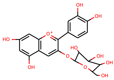
Figure 1: Chemical structure of the cyanin molecule (C₂₁H₂₁O₁₁) used to validate the new features and algorithms implemented in turboTDDFT 2.0

4.1 turboDavidson

In the left panel of Fig. 2 we compare the spectra computed for cyanin in the visible range, using the LBOA and the newly implemented turboDavidson algorithm. The LBOA calculation was performed using 3000 Lanczos iterations per polarization, while 15 Liouvillian eigentriplets were computed with turboDavidson. 9 iterations were sufficient in this case to abate the estimated error in the eigenvalues below $10^{-4}$ Ry. The total number of Liouvillian builds is twice the number of iterations in LBOA, while it is equal to the number of (right or left) unconverged eigenvectors per iteration in turboDavidson (less than 250 in total in present case). This substantial saving in computer time (at the cost of a substantial increase in the memory needed by Davidson algorithms) is typical of all those cases where one is interested in the optical spectrum over a restricted energy range, with only a few discrete transitions occurring therein.

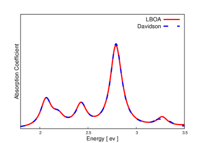
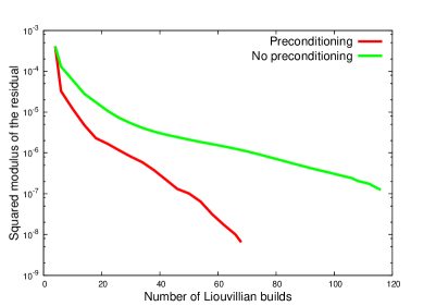
Figure 2: Left panel: Comparison of the spectra of cyanin calculated by the LBOA and our turboDavidson algorithm. Right panel: squared norm of the residual vector for the lowest excitation energy of cyanin versus the number of Liouvillian builds.

The present Davidson algorithm is a variant of the one introduced in Ref. [29], featuring a newly introduced preconditioning (see Eq. (32)) that dramatically improves upon the performances of the original algorithm. This improvement is illustrated in the right panel of Fig.2 that reports the magnitude of the squared modulus of the residual (line 10 in algorithm box 3) as a function of the number of Liouvillian builds, with and without preconditioning.

4.2 Pseudo-Hermitian Lanczos

In the left panel of Fig. 3 we compare the spectra computed for cyanin using two different flavors of the Lanczos algorithm: the LBOA and the newly introduced PHLA. We see that the substantial saving in the number of Liouvillian builds realized by the PHLA (a factor of two per iteration, with respect to other LBOA) does not compromise on the accuracy, if not for a marginal increase in the number of iterations needed to achieve a target accuracy (a few percent in our experience).

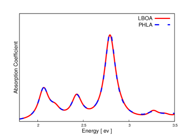
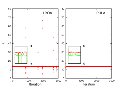
Figure 3: Left panel: Comparison of the spectra of cyanin calculated by the LBOA and the PHLA. Right panels: beta coefficients generated by the LBOA (left) and PHLA (right) algorithms. In the inset, the same data are shown on a magnified scale and with different colors for odd (red) and even (green) coefficients.

As it was discussed in Sec. 2.3, the LBOA is subject to quasi-breakdowns occurring whenever a newly generated pair of (left and right) vectors are almost orthogonal. When a quasi-breakdown occurs, the newly generated $\beta$ coefficient (see Algorithm box 1) suddenly blows up, as illustrated in the middle panel of Fig. 3. As it is typical of numerical instabilities in Lanczos-like algorithms, the occurrence of quasi-breakdowns depends on a number numerical details of the calculation (such as size of the super-cell, the kinetic-energy cutoff, or even the computer arithmetic). Fortunately, to the best of our knowledge and experience, the quality of the computed spectrum is rather insensitive to these numerical details and to the resulting instabilities. This being said, it is relieving that such a simple fix as the the PHLA, which results in a substantial reduction of computer time, also completely eliminates these instabilities, as it is demonstrated in the right panel of Fig. 3.

4.3 Hybrid functionals

In Fig. 4 we compare the optical spectra calculated with the PBE0 functional using a PW basis set and the present implementation of the Davidson algorithm with those obtained with a Gaussian basis set and the Gaussian 09 code. The two spectra match almost perfectly, the residual discrepancies being likely due to the slight inconsistency introduced by using a PBE pseudo-potential [34] with a PBE0 functional.

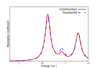
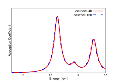
Figure 4: Left panel: Absorption spectra of cyanin, calculate by turboDavidson and Gaussian09, respectively. Right panel: comparison of the spectra calculated with the turboTDDFT code using several different values of ecutfock.

As the action of the $V_{EXX}$ operator requires the evaluation of the convolution of products of pairs of one-electron wave-functions with the Coulomb kernel (see Eq. (15)), one could expect that these operations require a PW cut-off four times as large as the wavefunction cut-off. The discussion in Sec. 2.4, however, suggests that the overall accuracy of a response calculation may be rather insensitive to the value of the PW cutoff employed for evaluating the $V_{EXX}$ operator, ecutfock. In the right panel of Fig. 4 we display the spectra obtained using a value for ecutfock ranging from the value used for the Kohn-Sham orbitals to four times as much, and demonstrates that setting $\texttt{ecutfock}=\texttt{ecutwfc}$ does not result in any significant loss of accuracy, and this value is therefore assumed as the default one.

5 Conclusions

In this paper we have introduced three substantial improvements and generalizations to the algorithms implemented in the turboTDDFT code for computing excited-state properties within linearized TDDFT. First and foremost, turboTDDFT 2.0 allows to use hybrid functionals, which substantially improve upon the accuracy attainable by semilocal PBE-like functionals. Second, it is now possible to compute individual excitation energies and amplitudes using a variant of the Davidson algoritm. Finally, our Liouville-Lanczos approach to the computation of optical spectra has been substantially improved by adopting a recently proposed pseudo-Hermitian variant to it. Work is in progress to remove the present limitation of hybrid functionals to norm-conserving pseudo-potentials, to unify the approaches to hybrid functionals and to the Bethe-Salpeter equation, and to further improve the overall numerical efficiency of the algorithms implemented in the turboTDDFT code.

Appendix A Input Variables

Card	Variable name Default Value Description
lr_input	prefix ’pwscf’ The files generated by the ground state pw.x run should have this same prefix. outdir ’./’ Working directory. On start, it should contain the files generated by a ground state pw.x run. wfcdir unset Directory for scratch data. restart .false. When set to .true., turbo_lanczos.x will attempt to restart from a previous interrupted calculation. (see restart_step variable). restart_step itermax The code writes restart files every restart_step iterations. Restart files are automatically written at the end of itermax Lanczos steps. lr_verbosity 1 Verbosity level
lr_control	itermax 500 Number of iterations to be performed. ipol 1 Component of the polarizability tensor to be computed: $1\rightarrow(xx)$, $2\rightarrow(yy)$, $3\rightarrow(zz)$. When set to 4 the full polarizability tensor is computed. nipol 1 if ipol $<$ 4; 3 if ipol=4 Determines the number of zeta coefficients to be calculated for a given polarization direction. ltammd .false. When set to .true. the Tamm-Dancoff approximation is used. no_hxc .false. When set to .true. the response of the Hartree and XC potentials are ignored, resulting in an independent-electron approximation. d0psi_rs .false. When set to .true., the matrix elements of the dipole operator are calculated in real space. Can be used only for molecules or clusters, NOT for periodic systems. Molecule must be placed in the centre of the simulation cell. It is recommended to set this value only for hybrid-functional calculations. ecutfock $4\times\texttt{ecutwfc}$ PW cut-off to compute EXX-like terms. charge_response 0 When set to 1, the code computes and writes the response charge density. Setting charge_response to 1 makes the presence of the card lr_post mandatory. pseudo_hermitian .true. Setting this parameter to .false. one can use the LBOA as in turboTDDFT 1.0.
lr_post	omeg 0.0 The response of the charge density is calculated for this transition energy (in Rydberg units) epsil 0.0 The broadening/damping term (in Rydberg units). beta_gamma_z_prefix ’pwscf’ The prefix of the file where the beta gamma zeta coefficients from the first calculation can be set manually using this parameter. The file outdir/beta_gamma_z_prefix.beta_gamma_z.x (where x=1-3) must exist. w_T_npol 1 Number of polarization directions considered in the previous calculation. It must be set to 3 if in the previous calculation ipol=4, it must be set to 1 otherwise. plot_type 1 An integer variable that determines the format of the file containing the charge density response. 1: A file containing the x y z grid coordinates and the corresponding value of the density is produced 2: The density response is written in Xcrysden format 3: The density response is written in the gaussian cube format

Table 1: Input variables for turbo_lanczos.x

Card	Variable name Default Value Description
lr_input	prefix ’pwscf’ Sets the prefix for generated and read files. The files generated by the ground state pw.x run should have this same prefix. outdir ’./’ The directory that contains the run critical files, which include the files generated by ground state pw.x run.. wfcdir unset The directory where the scratch files will be written and read. Restart related files are always written to outdir.
lr_dav	num_eign 1 Number of eigenstates to be calculated. num_init 2 Number of trial vectors. if_random_init .false. When set to $.true.$ trial vectors are chosen randomly, otherwise they are guessed from ground-state calculation. If $N_{v}N_{c}<num\_init$, this term is forced to be $.true.$. num_basis_max 20 Maximum number of basis vectors allowed in the subspace. When this number is reached, a discharging routine is called, sorting out $2\times num\_eign$ best vectors in the subspace and dumping the others. reference 0.0 $\omega_{ref}$ (Ry) is used to favor these eigenstates which have $\omega$’s the closest to this value. residue_conv_thr $10E-4$ Threshhold for the convergence. When the square of the residue is smaller than this value, the convergence is achieved. start 0 The lower limit of the energy (Ry) scale for the spectrum calculation. finish 1 The upper limit of the energy (Ry) scale for the spectrum calculation. broadening 0.005 Value (Ry) to broaden the spectrum. step 0.001 Energy step (Ry) for the spectrum calculation. ltammd .false. When set to .true. the Tamm-Dancoff approximation is used in constructing the Liouvillian. no_hxc .false. When set to .true. the change in the internal field (Hartree and exchange-correlation) is ignored in the calculation, resulting in an independent electron approximation. ecutfock ecutwfc The charge density cut-off of the reduced grid used to calculate the EXX-like operators. d0psi_rs .false. When set to .true., the matrix elements of dipole operator are calculated in real space. Can be used only for molecules or clusters, NOT for periodic systems. Molecule must be placed in the centre of the simulation cell. It is recommended to set this value only for hybrid-functional calculations.

Table 2: Input variables for turbo_davidson.x

Appendix B Sample inputs

&control
    calculation=’scf’
    restart_mode=’from_scratch’,
    pseudo_dir = ’./pseudo’,
    outdir=’./out’
    prefix=’CO’
/
&system
    ibrav= 1,
    celldm(1)=20,
    nat=  2,
    ntyp= 2,
    ecutwfc = 40
    ecutfock=40
    input_dft=’PBE0’
    nosym=.true.
    x_gamma_extrapolation=.false.
    exxdiv_treatment=’vcut_spherical’
/
&electrons
    adaptive_thr=.true.
    conv_thr=1d-10
/
ATOMIC_SPECIES
 C 1.0 C.pbe-mt_gipaw.UPF
 O 1.0 O.pbe-mt.UPF
ATOMIC_POSITIONS {angstrom}
  CΨ5.000Ψ5.000Ψ4.436
  OΨ5.000Ψ5.000Ψ5.564
K_POINTS {gamma}

Input sample for pw.x calculation of a CO molecule using the PBE0 functional, as documented in the PWscf input guide in the Quantum ESPRESSOdistribution.

&lr_input
    prefix="CO",
    outdir=’./out’,
    restart_step=500,
/
&lr_control
    itermax=1000,
    ipol=4,
    ecutfock=40d0 !This value has to be the same as in the scf input
    pseudo_hermitian=.true.
    d0psi_rs = .true.
/

Input sample for turbo_lanczos.x

&lr_input
    prefix="CO",
    outdir=’./out’,
/
&lr_dav
    ecutfock=40d0,
    num_eign=20,
    num_init=40,
    num_basis_max=200,
    residue_conv_thr=1.0E-4,
    start=0.0,
    finish=1.0,
    step=0.001,
    broadening=0.005,
    reference=0.0
    d0psi_rs = .true.
/

Input sample for turbo_davidson.x

References

- [1] E. Runge and E. K. U. Gross, Phys. Rev. Lett 52 (1984) 997.
- [2] Fundamentals of Time-Dependent Density Functional Theory, edited by M. A. L. Marques, N. T. Maitra, F. M. S. Nogueira, E. K. U. Gross, and A. Rubio, (Lecture Notes in Physics, Vol. 837, Springer-Verlag, Berlin Heidelbnerg, 2012).
- [3] B. Walker, A. Saitta, R. Gebauer, and S. Baroni, Phys. Rev. Lett. 128 (2006) 113001.
- [4] D. Rocca, R. Gebauer, Y. Saad, and S. Baroni, J. Chem. Phys. 128 (15) (2008) 154105.
- [5] S. Baroni, R. Gebauer, O. B. Malcıoğlu, Y. Saad, P. Umari, J. Xian, J. Phys.: Condens. Matt. 22 (2010) 074204.
- [6] S. Baroni and R. Gebauer, Ref. [2], chapter 19, pp. 375-390.
- [7] O. B. Malcıoğlu, R. Gebauer, D. Rocca, and S. Baroni, Comp. Phys. Commun. 182 (8) (2011) 1744-1754.
- [8] P. Giannozzi, S. Baroni, et al. J. Phys.: Condens. Matt. 21 (39) (2009) 395502.
- [9] A.J. Cohen, P. Mori-Sánchez, W. Yang, Chem. Rev. 112 (2012) 289–320.
- [10] A. Dreuw, J.L. Weisman, M. Head-Gordon, J. Chem. Phys. 119 (2003) 2943.
- [11] D. Rocca, D. Lu, G. Galli, J. Chem. Phys. 133 (16) (2010) 164109.
- [12] P. Ghosh, R. Gebauer, J. Chem. Phys. 132 (2010) 104102.
- [13] G. Onida, L. Reining, A. Rubio, Rev. Mod. Phys. 74 (2002), 601-659.
- [14] A.D. Becke, J. Chem. Phys. 98 (2) (1993) 1372-1377.
- [15] A. D. McLachlan, and M. A. Ball, Rev. Mod. Phys. 36 (1964) 844-855.
- [16] D. Rocca, Y. Ping, R. Gebauer, and G. Galli, Phys. Rev. B 85 (2012) 045116.
- [17] M. Grüning, A. Marini, and X. Gonze, Comput. Mat. Sci., 50 (2011) 2148-2156.
- [18] E. R. Davidson, J. Comp. Phys., 17 (1975) 87-94.
- [19] S. Baroni, P. Giannozzi, and A. Testa, Phys. Rev. Lett. 58 (1987) 1861.
- [20] S. Baroni, S. de Gironcoli, A. Dal Corso, and P. Giannozzi, Rev. Mod. Phys. 73 (2001) 515.
- [21] See, e.g., G. H. Golub and C. F. V. Loan, Matrix Computations, 3rd ed. (Johns Hopkins University Press, Baltimore, MD, 1996), p. 503.
- [22] M. Marsili and P. Umari, Phys. Rev. B 87 (2013) 205110.
- [23] C. Adamo and V. Barone, J. Chem. Phys. 110 (1999) 6158.
- [24] J. P. Perdew, K. Burke, and M. Ernzerhof, Phys. Rev. Lett. 77 (1996) 3865.
- [25] D.J. Thouless, Nucl. Phys. 21 (1960) 225–232.
- [26] A. Mostafazadeh, J. Math. Phys. 43 (2002) 205.
- [27] A. Mostafazadeh, J. Math. Phys. 43 (2002) 3944.
- [28] J. Hutter, J. Chem. Phys. 118 (2003) 3928–3934.
- [29] S. Tretiak, C.M. Isborn, A.M.N. Niklasson, and M. Challacombe, J. Chem. Phys. 130 (2009) 54111.
- [30] S. Hirata and M. Head-Gordon, Chem. Phys. Lett. 314 (1999) 291.
- [31] S. Rettrup, J. Comput. Phys. 45 (1982) 100.
- [32] J.P. Perdew, K. Burke, and M. Ernzerhof, Phys. Ref. Lett. 77 (1996) 3865-3868.
- [33] B. Walker and R. Gebauer, J. Chem. Phys. 127 (2007) 164106.
- [34] http://www.quantum-espresso.org/pseudopotentials/. The pseudopotentials adopted in these benchmarks are H.pbe-van_bm.UPF (H.pbe-vbc.UPF), C.pbe-van_bm.UPF (C.pbe-mt_gipaw.UPF), and O.pbe-van_bm.UPF, (O.pbe-mt.UPF), for H, C, and O atoms using the PBE (PBE0) functional.
- [35] R.E. Stratmann, G.E. Scuseria, M.J. Frisch, J. Chem. Phys. 109 (1998) 8218.